The Stability of the First Neumann Laplacian Eigenfunction Under Domain Deformations and Applications

Abstract.

The robustness of manifold learning methods is often predicated on the stability of the Neumann Laplacian eigenfunctions under deformations of the assumed underlying domain. Indeed, many manifold learning methods are based on approximating the Neumann Laplacian eigenfunctions on a manifold that is assumed to underlie data, which is viewed through a source of distortion. In this paper, we study the stability of the first Neumann Laplacian eigenfunction with respect to deformations of a domain by a diffeomorphism. In particular, we are interested in the stability of the first eigenfunction on tall thin domains where, intuitively, the first Neumann Laplacian eigenfunction should only depend on the length along the domain. We prove a rigorous version of this statement and apply it to a machine learning problem in geophysical interpretation.

1. Introduction and Main Result

1.1. Motivation

We are motivated by a machine learning problem in the field of geophysical interpretation: given a seismic image, the objective is to reparameterize depth in the image (the $y$-axis) such that each layer in the seismic image has constant depth. We propose an unsupervised diffusion based method to achieve this goal. In particular, we propose defining a discrete diffusion process that travels rapidly along the layers of a seismic image, and slowly perpendicular to the layers. This anisotropic diffusion process corresponds to an isotropic diffusion process on some tall thin domain formed by contracting the metric of the seismic image along its layers, see the illustration in Figure 1.

$\left(\begin{subarray}{c}\text{underlying}\\ \text{tall thin}\\ \text{domain}\end{subarray}\raisebox{-0.5pt}{ \includegraphics[height=55.64821pt]{idea3-eps-converted-to.pdf}}\qquad\right)$

$\overset{\text{output}}{\mapsto}$

Figure 1. Cartoon of a seismic image (left), underlying tall thin domain (center), and reparameterized image (right).

The first eigenfunction of this anisotropic diffusion operator is then used to reparameterize depth in the seismic image. Specifically, if the diffusion operator is defined with Neumann boundary conditions (as is standard for diffusion based machine learning methods [1]), then the first eigenfunction of the diffusion operator will approximate the first Neumann Laplacian eigenfunction of the underlying tall thin domain. In the ideal case, this underlying domain will be a tall rectangle, whose first Neumann Laplacian eigenfunction is $\cos(\pi y/h)$, where $h$ is the height of the rectangle. We can use this eigenfunction to assign each pixel in the seismic image its height in the underlying tall rectangle, thereby flattening the layers of the image.

1.2. Stability of the first Neumann eigenfunction

The main challenge in the proposed algorithm is constructing the anisotropic diffusion process, which rapidly travels along the layers of the given seismic image. Inaccuracies in the construction of this anisotropic diffusion process, will cause the underlying domain on which the anisotropic diffusion process is an isotropic diffusion process to be a deformed version of a tall rectangle. This issue motivates the following question: how stable is the first Neumann Laplacian eigenfunction under domain deformations? Numerically, we observe that on long thin domains, the Neumann Laplacian eigenfunctions demonstrate a high degree of stability with respect to domain deformations. To illustrate this idea, we compute the first Neumann Laplacian eigenfunction numerically on two different domains, and we visualize each eigenfunction on its respective domain using a color map, see Figure 2.

$\Omega_{1}$	$\Omega_{2}$

Figure 2. The first Neumann Laplacian eigenfunction on two different long thin domains.

To formalize a notion of stability, let $R\subset\mathbb{R}^{d}$ be an open bounded connected domain with a piecewise smooth boundary $\partial R$. Suppose that $R$ is transformed by a diffeomorphism $\varphi$ into a domain $\Omega:=\varphi(R)$. Let $0=\eta_{0}<\eta_{1}\leq\eta_{2}\leq\cdots$ and $v_{0},v_{1},v_{2},\ldots$ denote the Neumann Laplacian eigenvalues and eigenfunctions on $R$, and let $0=\mu_{0}<\mu_{1}\leq\mu_{2}\leq\cdots$ and $u_{0},u_{1},u_{2},\ldots$ denote the Neumann Laplacian eigenvalues and eigenfunctions on $\Omega$. More precisely, $\eta_{j},v_{j}$ and $\mu_{j},u_{j}$ are characterized by the following eigenvalue problems

$$\left\{\begin{array}[]{cc}-\Delta v_{j}=\eta_{j}v_{j}&\text{in }R\\ \frac{\partial}{\partial n}v_{j}=0&\text{on }\partial R\end{array}\right.\quad\text{and}\quad\left\{\begin{array}[]{cc}-\Delta u_{j}=\mu_{j}u_{j}&\text{in }\Omega\\ \frac{\partial}{\partial n}u_{j}=0&\text{on }\partial\Omega,\end{array}\right.$$

where $\Delta$ denotes the Laplacian, and $n$ denotes an outward normal to the boundary of the domain. We can now formulate precise questions about the stability of the first Neumann Laplacian eigenfunction. For example, we can consider the distance between $u_{1}\circ\varphi$ and $v_{1}$ with respect to the $L^{2}(R)$-norm. More generally, we can ask: how accurately can we represent $u_{1}\circ\varphi$ in the span of the first $k$ eigenfunctions $v_{1},\ldots,v_{k}$? Quantitative answers to these questions will provide some understanding of the stability of the first Neumann eigenfunction that we observe both numerically and in machine learning applications.

1.3. Preview of application results

The stability of the first Neumann eigenfunction is also evident in the application results. Given a seismic image, we construct a discrete diffusion process that travels rapidly along the layers of the image as described in §3. Given the high level of noise in the image, this anisotropic diffusion process cannot be defined perfectly, yet when we reparameterize depth in the image using the first eigenfunction of the diffusion, the layers are roughly flat, see Figure 9. Moreover, the reparameterized image actually encodes more detailed geometric information: by zooming into the interval $[0.6,1.2]$ on the $y$-axis of the reparameterized space, we observe that the individual layers of the image have been automatically separated by the reparameterization, which makes it possible to use post-processing to further refine the results.

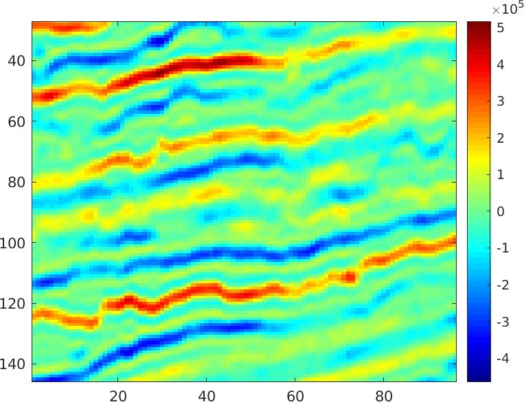
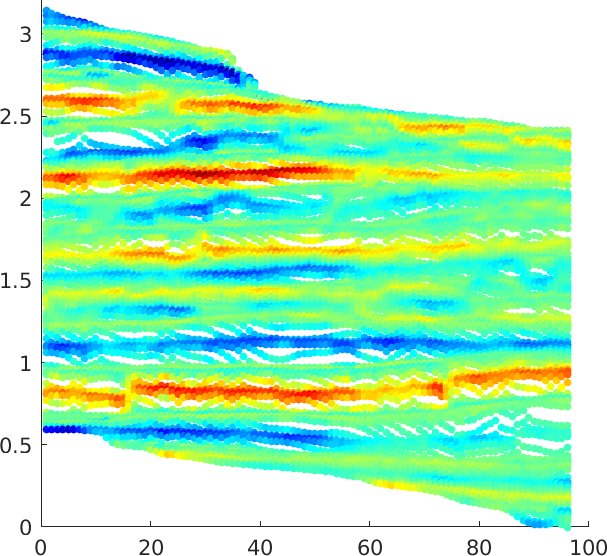
$\overset{\text{output}}{\mapsto}$ $\begin{subarray}{c}\text{zoomed}\\ \text{image}\end{subarray}\raisebox{-0.5pt}{ \includegraphics[height=73.7146pt]{zoomflat_a22.jpg}}$

Figure 3. Seismic image (left), result of diffusion based reparameterization (center), and zoomed image (right).

1.4. Main Result

Let $R\subset\mathbb{R}^{d}$ be an open bounded connected domain of unit measure with a piecewise smooth boundary $\partial R$. Suppose that $\varphi:R\rightarrow\Omega$ is a diffeomorphism, and suppose that $J(x)=\frac{\partial\varphi_{i}}{\partial x_{j}}(x)$ is the Jacobian matrix of this diffeomorphism. Let $0=\eta_{0}<\eta_{1}\leq\eta_{2}\leq\cdots$ and $v_{0},v_{1},v_{2},\ldots$ denote the Neumann Laplacian eigenvalues and eigenfunctions on $R$, respectively, and let $0=\mu_{0}<\mu_{1}\leq\mu_{2}\leq\cdots$ and $u_{0},u_{1},u_{2},\ldots,$ denote the Neumann Laplacian eigenvalues and eigenfunctions on $\Omega$, respectively. We refer to $R$ as the reference domain, and $\Omega$ as the deformed domain. For example, the domain $R$ may be some nice domain, where the Neumann Laplacian eigenfunctions are well understood, while $\Omega$ is a deformed version of this nice domain. To study the stability of the first Neumann Laplacian eigenfunction we will consider the quantity

$$\|(\operatorname{Id}-P_{V_{k}})u_{1}\circ\varphi\|_{L^{2}(R)},\quad\text{for}\quad k=1,2,\ldots,$$

where $\operatorname{Id}-P_{V_{k}}$ is the projection on the space orthogonal to $V_{k}=\operatorname{span}\{v_{1},\ldots,v_{k}\}$. This quantity measures how much of the function $u_{1}\circ\varphi$ cannot be represented in the linear span of the first $k$ Neumann Laplacian eigenfunctions $v_{1},\ldots,v_{k}$. In Remark 1.1, we describe how bounds on the quantity $\|(\operatorname{Id}-P_{V_{k}})u_{1}\circ\varphi\|_{L^{2}(R)}$ can be used to understand the observed stability of the first Neumann Laplacian eigenfunction on tall thin domains.

Theorem 1.1.

Suppose that the singular values of the Jacobian matrix $J(x)$ are contained in the interval $(1-\varepsilon,1+\varepsilon)$ on $R$, and suppose that $0\leq\varepsilon d\leq 1/10$. Then,

$$\left\|\left(\operatorname{Id}-P_{V_{k}}\right)u_{1}\circ\varphi\right\|_{L^{2}(R)}^{2}\leq 20\frac{\eta_{1}\varepsilon d}{\eta_{k+1}-\eta_{1}}+\varepsilon d,$$

where $\operatorname{Id}-P_{V_{k}}$ denotes the projection on the space orthogonal to $V_{k}:=\operatorname{span}\{v_{1},\ldots,v_{k}\}$.

Informally speaking, Theorem 1.1 says that if the deformation $\varphi$ is small and the gap $\eta_{k+1}-\eta_{1}$ is large, then the function $u_{1}\circ\varphi$ is roughly contained in the linear span of the first $k$ Neumann Laplacian eigenfunctions $v_{1},\ldots,v_{k}$. We note that the constants appearing in the statement of Theorem 1.1 have not been optimized, and are for illustrative purposes. Furthermore, we remark that the term $\varepsilon d$ that appears in the right hand side of the above inequality can be removed if instead of $\|(\operatorname{Id}-P_{V_{k}})u_{1}\circ\varphi\|_{L^{2}(R)}$, we consider the quantity $\|(\operatorname{Id}-P_{\overline{V}_{k}})u_{1}\circ\varphi\|_{L^{2}(R)}$, where $\overline{V}_{k}=\operatorname{span}\{v_{0},v_{1},\ldots,v_{k}\}$. In the following remark, we apply Theorem 1.1 to understand the case where the reference domain is a tall rectangle.

Remark 1.1 (Tall thin reference domain).

Suppose that the rectangle $R=[0,1/10]\times[0,10]\subset\mathbb{R}^{2}$ is given. For this rectangle, the first $100$ Neumann Laplacian eigenfunctions $v_{1},\ldots,v_{100}$ are functions of only the $y$-variable (which varies in the vertical direction). In particular, these eigenfunctions are of the form $\cos(\pi jy/10)$, for $j=1,\ldots,100$. If we include the constant eigenfunction $v_{0}$, and define $\overline{V}_{100}=\operatorname{span}\{v_{0},v_{1},\ldots,v_{100}\}$, then by the discussion following Theorem 1.1 we have,

$$\left\|\left(\operatorname{Id}-P_{\overline{V}_{100}}\right)u_{1}\circ\varphi\right\|_{L^{2}(R)}^{2}\leq 20\frac{2(\pi^{2}/10^{2})\varepsilon}{\pi^{2}10^{2}-\pi^{2}}<\frac{\varepsilon}{200},$$

when $\varepsilon>0$ is sufficiently small. Moreover, since the first $100$ Neumann Laplacian eigenfunctions are functions of the $y$-variable, the above inequality has an interesting consequence. Let $V$ denote the span of all functions on the rectangle that only depend on the $y$-variable, and set $P_{H}=\operatorname{Id}-P_{V}$. Then,

$$\left\|P_{H}u_{1}\circ\varphi\right\|_{L^{2}(R))}<\frac{\varepsilon}{200}.$$

That is to say, the function $u_{1}\circ\varphi$ is essentially a function of the $y$-variable of the underlying tall thin rectangle, and it has very little variation in the horizontal direction. As a consequence, level sets of the function $u_{1}\circ\varphi$ are approximately horizontal lines.

1.5. Diffusion geometry methods

Our approach falls under the class of diffusion geometry machine learning methods, which are popular methods of organizing data that have a theoretical basis in analysis. Diffusion geometry methods originated with Diffusion Maps [1], and are based on constructing a diffusion operator on data whose eigenfunctions encode the pertinent geometric information for the given application, see for example [2, 3, 4, 5, 6, 7]. In this paper we present a specialized construction of a diffusion operator whose first eigenfunction can be used to organize the layers within a seismic image. To justify the robustness of the proposed method, we study the stability of these eigenfunction under domain deformations. Our main result, Theorem 1.1, acts as a first step to understanding the stability of the algorithm. Diffusion geometry methods are highly related to other spectral methods such as Laplacian eigenmaps [8], and Theorem 1.1 also serves to partially illuminate such techniques.

1.6. Manifold Straightening

Let us reiterate the main idea of the application using the language of manifold learning. Suppose that $\mathcal{M}$ is a manifold whose metric is given locally, but for which no global coordinates are given. Furthermore, suppose that the manifold has a smooth vector field, which provides an orientation to each neighborhood. Assume that the given manifold is a distorted version of an underlying manifold where the vector field is constant, i.e, all vectors point in the same direction. Our objective is to recover the coordinates for this underlying intrinsic manifold. Our approach has three basic steps:

1. Contract the metric in the direction of the vector field.

2. Compute the first Neumann Laplacian eigenfunction on the stretched domain.

3. Use this Neumann Laplacian eigenfunction to recover the height variable on the underlying manifold.

Figure 4. Cartoon of a manifold with a vector field (left), and result of contracting the metric along the vector field (right).

In particular, when the underlying domain is approximately shaped like a tall rectangle, the height variable can be recovered from the eigenfunction using the $\arccos$ function.

1.7. Organization

The remainder of the paper is organized as follows. In §2 we introduce notation, outline the main idea of the proof of the Theorem, and provide a detailed proof. In §3 we introduce the application problem, outline the main idea of the algorithm, and display results. In A, the details of the data adaptive smoothing method, diffusion operator construction, and reparameterization method are provided.

2. Proof of main result

2.1. Notation and preliminaries

Suppose that $R$ is an open bounded connected subset of $\mathbb{R}^{d}$ of unit measure with a piecewise smooth boundary $\partial R$. We say that $0=\eta_{0}<\eta_{1}\leq\eta_{2}\leq\cdots$ and $v_{0},v_{1},v_{2},\ldots$ and the Neumann Laplacian eigenvalues and eigenfunctions, respectively, if they are solutions to the boundary value problem

$$\left\{\begin{array}[]{cc}-\Delta v_{j}=\eta_{j}v_{j}&\text{in }R\\ \frac{\partial}{\partial n}v_{j}=0&\text{on }\partial R,\end{array}\right.$$

where $n$ denotes an outward normal to the boundary of the domain. Suppose that $\varphi:R\rightarrow\Omega$ is a diffeomorphism, and let $0=\mu_{0}<\mu_{1}\leq\mu_{2}\leq\cdots$ and $u_{0},u_{1},u_{2},\ldots$ denote the Neumann Laplacian eigenvalues and eigenfunctions on $\Omega$, respectively. Let $J(x)=\frac{\partial\varphi_{i}}{\partial x_{j}}(x)$ denote the Jacobian matrix of the diffeomorphism $\varphi$. If $y:=\varphi(x)$ and $u\in C^{1}(\Omega)$, then the chain rule can be expressed by

$$J^{T}(\varphi^{-1}(y))\nabla_{y}u(y)=\nabla_{x}u(\varphi(x)),$$

where

$$\nabla_{y}=\left(\frac{\partial}{\partial y_{1}},\frac{\partial}{\partial y_{2}}\right)^{\top}\quad\text{and}\quad\nabla_{x}=\left(\frac{\partial}{\partial x_{1}},\frac{\partial}{\partial x_{2}}\right)^{\top}.$$

Similarly, given a function $v\in C^{1}(R)$, the chain rule can be expressed by

$$(J^{-1})^{T}(\varphi^{-1}(x))\nabla_{x}v(x)=\nabla_{y}v(\varphi(y)).$$

Let $\det J(x)$ denote the Jacobian determinant such that

$$\int_{\Omega}u(y)dy=\int_{R}u(\varphi(x))|\det J(x)|dx,\quad\text{and}\quad\int_{R}v(x)dx=\int_{\Omega}v(\varphi^{-1}(y))|\det J^{-1}(y)|dy.$$

The assumption that the singular values of $J(x)$ are contained in the interval $[1-\varepsilon,1+\varepsilon]$ on $R$ implies that

$$(1-\varepsilon)^{d}\leq\det J(x)\leq(1+\varepsilon)^{d}.$$

Recall the following two classical inequalities involving Euler’s number $e$:

$$\left(1+\frac{1}{x}\right)^{x}<e\quad\text{and}\quad e^{-1}<\left(1-\frac{1}{x}\right)^{x-1},\quad\text{for all}\quad 1<x<\infty.$$

It follows directly from Taylor’s Inequality that

$$|e^{x}-1|<e^{1/10}x\quad\text{when}\quad|x|<\frac{1}{10}.$$

Therefore, assuming that $\varepsilon d<1/10$, it follows that

$$(1+\varepsilon)^{d}=(1+\varepsilon)^{\frac{\varepsilon d}{\varepsilon}}\leq e^{\varepsilon d}<1+e^{1/10}\varepsilon d<1+2\varepsilon d,$$

and similarly that,

$$(1-\varepsilon)^{d}=(1-\varepsilon)^{\left(\frac{1}{\varepsilon}-1\right)\left(\frac{\varepsilon}{1-\varepsilon}\right)d}>e^{-\frac{\varepsilon}{1-\varepsilon}d}>1-e^{1/10}\frac{\varepsilon}{1-\varepsilon}d>1-2\varepsilon d.$$

By combining these inequalities we conclude that if the singular values of $J(x)$ are contained in the interval $[1-\varepsilon,1+\varepsilon]$ on $R$, and $0\leq\varepsilon d<1/10$, then

$$1-2\varepsilon d\leq\det J(x)\leq 1+2\varepsilon d.$$

In the following, while establishing the lemmas involved in the proof of Theorem 1.1, we will assume that the singular values of $J(x)$ are contained in the interval $[1-\varepsilon,1+\varepsilon]$, and will assume that

$$1-\delta\leq\det J(x)\leq 1+\delta.$$

Then, to complete the proof of Theorem 1.1, we will substitute $\delta=2\varepsilon d$. In addition to simplifying notation, controlling the determinant and singular values of $J(x)$ separately is useful for understanding certain classes of transformations; for example, the shear transform

$$(x_{1},x_{2})\overset{\varphi}{\mapsto}(x_{1}+\alpha x_{2},x_{2}),$$

has arbitrarily large singular values as $\alpha\rightarrow\infty$, but has Jacobian matrix

$$J(x)=\left(\begin{array}[]{cc}1&\alpha\\ 0&1\end{array}\right),$$

which has determinant $1$.

2.2. Outline of the proof of Theorem 1.1

Let $\gtrsim$ denote $\geq$ up to multiplication by a constant equal to $1+O(\varepsilon)$. Recall that $\eta_{j}$ and $v_{j}$ are the Neumann Laplacian eigenvalues and eigenfunctions on $R$, while $\mu_{j}$ and $u_{j}$ are the Neumann Laplacian eigenvalues and eigenfunctions on $\Omega$. Observe that the condition that the singular values of $J(x)$ are contained in the interval $[1-\varepsilon,1+\varepsilon]$ on $R$ can be succinctly stated as

$$\sigma\left(JJ^{\top}\right)\subset\left[(1-\varepsilon)^{2},(1+\varepsilon)^{2}\right].$$

The proof of Theorem 1.1 is divided into three lemmas. First, in Lemma 2.1 we will show

$$\eta_{1}=\|\nabla_{x}v_{1}\|^{2}_{L^{2}(R)}\gtrsim\|\nabla_{y}(v_{1}\circ\varphi^{-1})\|_{L^{2}(\Omega)}^{2}\gtrsim\inf_{u\perp 1:\|u\|=1}\|\nabla_{y}u\|_{L^{2}(\Omega)}^{2}=\mu_{1},$$

where the infimum is taken over sufficiently smooth functions of unit $L^{2}(\Omega)$-norm, which are orthogonal to constant functions on $L^{2}(\Omega)$. Second, in Lemma 2.2 we will show that

$$\mu_{1}=\|\nabla_{y}u_{1}\|_{L^{2}(\Omega)}^{2}\gtrsim\|\nabla_{x}(u_{1}\circ\varphi)\|_{L^{2}(R)}^{2}=\sum_{j=1}^{\infty}\eta_{j}\alpha_{j}^{2},$$

where $\alpha_{j}$ are the coefficients of $u_{1}\circ\varphi$ expanded in the orthogonal basis $\{v_{j}\}$ of Neumann eigenfunctions on $R$. Third, in Lemma 2.3 we show that $\alpha_{0}^{2}$ is $\mathcal{O}(\varepsilon^{2})$. Finally, in §2.4 we combine these lemmas to conclude that

$$\eta_{1}\gtrsim\sum_{j=1}^{\infty}\eta_{j}\alpha_{j}^{2},$$

and then we use this inequality to control how large the coefficients $\alpha_{j}^{2}$ can be. In particular, since $\eta_{j}$ is increasing, observe that this inequality provides increasing control as $j$ increases.

2.3. Lemmas involved in the proof of Theorem 1.1

Lemma 2.1.

Suppose that $\sigma\left(JJ^{\top}\right)\subset\left[(1-\varepsilon)^{2},(1+\varepsilon)^{2}\right]$ and $|\det J(x)-1|<\delta$ on $R$. Then,

$$\eta_{1}\frac{(1+\varepsilon)^{2}(1-\delta)}{(1-\delta)^{3}-(1+\delta)\delta^{2}}\geq\mu_{1}.$$

Proof.

Multiplying the equation $\Delta v_{1}+\eta_{1}v_{1}=0$ by $v_{1}$, integrating over $R$, and applying Green’s Identity yields

$$\eta_{1}=\|\nabla_{x}v_{1}\|_{L^{2}(R)}^{2},$$

which by the chain rule, and a change of variables of integration is equivalent to

$$\eta_{1}=\|J^{T}\circ\varphi^{-1}\nabla_{y}\circ\varphi^{-1}\sqrt{|\det J^{-1}|}\|_{L^{2}(\Omega)}^{2}.$$

Therefore, by the assumed bounds for $\sigma_{\text{max}}(J)$ and $\det J$, we conclude that

$$\eta_{1}\frac{(1+\varepsilon)^{2}}{1-\delta}\geq\|\nabla_{y}v_{1}\circ\varphi^{-1}\|_{L^{2}(\Omega)}^{2}.$$

By the minimax principle, we have

$$\mu_{1}=\inf_{u\perp 1}\frac{\|\nabla_{y}u\|^{2}_{L^{2}(\Omega)}}{\|u\|_{L^{2}(\Omega)}^{2}},$$

where the infimum is taken over differentiable functions $u$, which are orthogonal to constant functions on $L^{2}(\Omega)$. It follows that

$$\frac{\|\nabla(v_{1}\circ\varphi^{-1}-c)\|_{L^{2}(\Omega)}^{2}}{\|v_{1}\circ\varphi^{-1}-c\|_{L^{2}(\Omega)}^{2}}\geq\mu_{1},$$

where $c$ is a constant such that the function $v_{1}\circ\varphi^{-1}-c$ is orthogonal to constant functions on $L^{2}(\Omega)$, i.e.,

$$c=\frac{1}{\|\Omega|}\int_{\Omega}v_{1}\circ\varphi^{-1}dx.$$

Now, combining this inequality with the previous inequality comparing $\eta_{1}$ and $\|\nabla_{y}v_{1}\circ\varphi^{-1}\|_{L^{2}(\Omega)}^{2}$ yields

$$\eta_{1}\frac{(1+\epsilon)^{2}}{(1-\delta)}\frac{1}{\|v_{1}\circ\varphi^{-1}-c\|_{L^{2}(\Omega)^{2}}^{2}}\geq\frac{\|\nabla_{y}(v_{1}\circ\varphi^{-1}-c)\|_{L^{2}(\Omega)}^{2}}{\|v_{1}\circ\varphi^{-1}-c\|_{L^{2}(\Omega)}^{2}}\geq\mu_{1}.$$

To complete the proof, it remains to compute a lower bound on $\|v_{1}\circ\varphi^{-1}-c\|_{L^{2}(\Omega)}^{2}$. The constant $c$ can be computed by taking the inner product of $v_{1}\circ\varphi^{-1}$ with the constant function $|\Omega|^{-1}$, specifically,

$$c=|\Omega|^{-1}\int_{\Omega}v_{1}(\varphi^{-1}(y))dy = |\Omega|^{-1}\int_{R}v_{1}(x)|\det J(x)|dx$$

$$\leq \delta|\Omega|^{-1}\int_{R}|v_{1}(x)|dx\leq\delta|\Omega|^{-1}|R|\leq\frac{\delta}{1-\delta}.$$

Since $v_{1}\circ\varphi^{-1}-c$ is orthogonal to constant functions in $L^{2}(\Omega)$,

$$\|v_{1}\circ\varphi^{-1}-c\|^{2}_{L^{2}(\Omega)} = \|v_{1}\circ\varphi^{-1}\|_{L^{2}(\Omega)}-\|c\|^{2}_{L^{(}\Omega)}$$

$$\geq \int_{R}|v_{1}(x)|^{2}|\det J(x)|dx-|\Omega|\left(\frac{\delta}{1-\delta}\right)^{2}$$

$$\geq (1-\delta)-(1+\delta)\frac{\delta^{2}}{(1-\delta)^{2}}$$

$$= \frac{(1-\delta)^{3}-(1+\delta)\delta^{2}}{(1-\delta)^{2}}.$$

Substituting this lower bound into our previous inequality yields:

$$\eta_{1}\frac{(1+\varepsilon)^{2}(1-\delta)}{(1-\delta)^{3}-(1+\delta)\delta^{2}}\geq\mu_{1}.$$

∎

Lemma 2.2.

Suppose that $\sigma\left(JJ^{\top}\right)\subset\left[(1-\varepsilon)^{2},(1+\varepsilon)^{2}\right]$ and $|\det J(x)-1|<\delta$ on $R$. Then,

$$\mu_{1}\frac{(1+\delta)}{(1-\varepsilon)^{2}}\geq\sum_{j=1}^{\infty}\eta_{j}\alpha_{j}^{2},$$

where $\alpha_{j}$ are the coefficients of $u_{1}\circ\varphi$ expanded in the orthogonal basis of eigenfunctions $\{v_{j}\}$ on $L^{2}(R)$.

Proof.

First, we express $\mu_{1}$ in terms of an integral of the function $\mu_{1}\circ\varphi$ over $R$,

$$\mu_{1}=\left\|(J^{-1})^{T}\circ\varphi\nabla_{x}(u\circ\varphi)\sqrt{|\det J|}\right\|_{L^{2}(R)}^{2}.$$

This construction is symmetric to our equation for $\eta_{1}$ in terms of an integral of $v_{1}\circ\varphi^{-1}$ over $\Omega$. Applying the bounds on $\sigma_{\text{min}}(J)$ and $\det J$ yields

$$\mu_{1}\frac{(1+\delta)}{(1-\varepsilon)^{2}}\geq\left\|\nabla_{x}(u_{1}\circ\varphi)\right\|_{L^{2}(R)}^{2}.$$

Since the Neumann Laplacian eigenfunctions $\{v_{j}\}$ form a orthonormal basis of $L^{2}(R)$, we can expand

$$u_{1}\circ\varphi(x)=\sum_{j=0}^{\infty}\alpha_{j}v_{j}(x),$$

where

$$\alpha_{j}=\int_{R}u_{1}(\varphi(x))v_{j}(x)dx.$$

By Green’s first identity, and the orthogonality of the eigenfunctions $\{v_{j}\}$, we have

$$\left\|\nabla_{x}\sum_{j=1}^{\infty}\alpha_{j}v_{j}\right\|_{L^{2}(R)}^{2}=\sum_{j=1}^{\infty}\eta_{j}\alpha_{j}^{2}.$$

Combining the previously developed inequalities and expanding $u_{1}\circ\varphi$ in $\{v_{j}\}$ establishes the inequality

$$\mu_{1}\frac{(1+\delta)}{(1-\varepsilon)^{2}}\geq\left\|\nabla_{x}(u_{1}\circ\varphi)\right\|_{L^{2}(R)}^{2}\geq\sum_{j=1}^{\infty}\eta_{j}\alpha_{j}^{2},$$

where $\alpha_{j}$ are the coefficients of $u_{1}\circ\varphi$ expanded in the orthogonal basis of eigenfunctions $\{v_{j}\}$ on $L^{2}(R)$. ∎

Observe that the sum in the inequality that we establish excludes the term $\eta_{0}\alpha_{0}^{2}$, as $\eta_{0}=0$. Therefore, our inequality offers no control over $\alpha_{0}^{2}$. However, since $u_{1}$ is orthogonal to constants on $L^{2}(\Omega)$, we suspect $u_{1}\circ\varphi$ is nearly orthogonal to constants on $L^{2}(R)$. In the following lemma, we formalize this intuition, and develop a precise bound for $\alpha_{0}^{2}$.

Lemma 2.3.

Suppose that $|\det J(x)-1|<\delta$ on $R$. Then,

$$\alpha_{0}^{2}\leq\frac{\delta^{2}(1+\delta)^{2}}{(1-\delta)^{2}}.$$

Proof.

By definition,

$$\alpha_{0}^{2}=\left(\int_{R}u_{1}(\varphi(x))dx\right)^{2}=\left(\int_{\Omega}u_{1}(y)|\det J^{-1}(y)|dy\right)^{2}.$$

Moreover, we have

$$\left(\int_{\Omega}u_{1}(y)|\det J^{-1}(y)|dy\right)^{2}\leq\left(\frac{\delta}{1-\delta}|\Omega|\right)^{2}\leq\frac{\delta^{2}(1+\delta)^{2}}{(1-\delta)^{2}},$$

which completes the proof. ∎

2.4. Proof of Theorem 1.1

In the following, we combine Lemmas 2.1, 2.2, and 2.3 to prove Theorem 1.1.

Proof of Theorem 1.1.

By combining the results of Lemma 2.1 and 2.2, we conclude that

$$\eta_{1}E_{\delta,\varepsilon}\geq\sum_{j=1}^{\infty}\eta_{j}\alpha_{j}^{2},$$

where

$$E_{\delta,\varepsilon}=\frac{(1+\varepsilon)^{2}}{(1-\varepsilon)^{2}}\frac{(1+\delta)(1-\delta)}{(1-\delta)^{3}-(1+\delta)\delta^{2}}.$$

Subtracting $\sum_{j=1}^{k}\eta_{j}\alpha_{j}^{2}$ from each side of this inequality yields

$$\eta_{1}E_{\varepsilon,\delta}-\sum_{j=1}^{k}\eta_{j}\alpha_{j}^{2}\geq\sum_{j={k+1}}^{\infty}\eta_{j}\alpha_{j}^{2}.$$

Then, since the eigenvalues $\eta_{1}\leq\eta_{2}\leq\eta_{3}\leq\cdots$ are in ascending order, we conclude that

$$\eta_{1}\left(E_{\varepsilon,\delta}-\sum_{j=1}^{k}\alpha_{j}^{2}\right)\geq\eta_{k+1}\sum_{j=k+1}^{\infty}\alpha_{j}^{2}.$$

By the inequality $1/(1+\delta)\leq\|u_{1}\circ\varphi\|_{L^{2}(R)}=\sum_{j=0}^{\infty}\alpha_{j}^{2}$, it follows that

$$\eta_{1}\left(E_{\varepsilon,\delta}-\left(\frac{1}{1+\delta}-\sum_{j=k}^{\infty}\alpha_{j}^{2}-\alpha_{0}\right)\right)\geq\eta_{k+1}\sum_{j=k+1}^{\infty}\alpha_{j}^{2}.$$

Rearranging and collecting terms gives

$$\frac{\eta_{1}F_{\varepsilon,\delta}}{\eta_{k+1}-\eta_{1}}\geq\sum_{j=k+1}^{\infty}\alpha_{j}^{2},$$

where

$$F_{\varepsilon,\delta}=\frac{(1+\varepsilon)^{2}}{(1-\varepsilon)^{2}}\frac{(1+\delta)(1-\delta)}{(1-\delta)^{3}+(1+\delta)\delta^{2}}+\frac{\delta^{2}(1+\delta)^{2}}{(1-\delta)^{2}}-\frac{1}{1+\delta}.$$

Let $\delta=2\varepsilon d$. Using Lemma 2.3, power series expansions, and assuming $\varepsilon d<1/10$ gives

$$20\frac{\eta_{1}\varepsilon d}{\eta_{k+1}-\eta_{1}}+\varepsilon d\geq\alpha_{0}^{2}+\sum_{j=k+1}^{\infty}\alpha_{j}^{2},$$

as was to be shown. ∎

3. Applications

3.1. Problem

In the field of geophysical interpretation, the problem of organizing the layers of a seismic image, otherwise known as seismic flattening, is of interest [9, 10, 11]. Given a seismic image, the objective is to modify the depth function of the seismic image such that each layer has constant depth. Since each layer was deposited at roughly the same time, the depth function which flattens the layers is sometimes referred to as geological time. In general, a seismic image consists of an $m\times n\times l$ real-valued tensor whose first coordinate is referred to as depth. As the depth increases, the values in the tensor oscillate between positive and negative values, but in a nonuniform way. For example in Figure 5 a two dimensional slice of a three dimensional seismic image is plotted using a color map, which exhibits this oscillating behavior.

Figure 5. Example of a two dimensional slice of a seismic image tensor.

In the following, we will primarily restrict our attention to such two dimensional slices of seismic tensors, except for the filtering process on the data, which does incorporate the pixels surrounding our two dimensional slice in the tensor.

3.2. Approach Outline

We approach the problem of seismic flattening from a diffusion geometry perspective. Given a seismic image, we construct a diffusion process whose eigenfunctions encode the geometric features of the data that are of interest, which, in this case, are the layers of the seismic image. Our method has three main steps:

1. Adaptive Filtering. A Principal Component Analysis filtering technique is used to associate filtered feature vectors to each pixel in the two dimensional seismic image. These filtered features incorporate information from the surrounding pixels.

2. Kernel Construction. A diffusion kernel is defined, which propagates rapidly along the layers of the seismic image and slowly perpendicular to these layers. This kernel is defined using the filtered feature vectors.

3. Layer Organization. The first eigenfunction of the diffusion operator (which should resemble the first Neumann Laplacian eigenfunction on the intrinsic underlying domain that is roughly shaped like a tall thin rectangle) is then used to organize the layers of the image.

Intuitively, since the constructed diffusion process propagates rapidly along the layers of the seismic image, and slowly perpendicular to the layers, if the diffusion operator is taken to a sufficient power, diffusion starting at a single point on a layer will completely propagate along the layer, with very little propagation perpendicular to the layer. This powered diffusion operator essentially replaces functions with their average along the layers of the seismic image. However, the eigenfunctions of the original diffusion operator and the powered diffusion operator are the same. Therefore, the first nontrivial eigenfunction of the diffusion operator must be essentially equal to its average on the layers of the image. That is to say, the first eigenfunction must be essentially constant on the layers of the image. A similar idea was used by Lafon, see Proposition 12 on page 47 of [1], where an anisotropic diffusion process is used to study differential systems.

3.3. Main idea

A complete description of the proposed method is provided in A. Here, we focus on explaining the kernel construction, which is the main idea of the proposed method. Suppose that the filtered feature vectors $f(i)$, which summarizes the structure of the seismic image at $i$, have already been computed using the method described in A. For each pixel $i$ we consider two spatial neighborhoods: a calibration neighborhood $C_{R}$, and a propagation neighborhood $N_{r}$, where $0<r<R$ denotes the radius of each neighborhood.

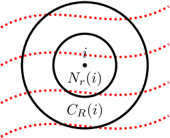
Figure 6. Illustration of propagation and calibration neighborhood.

The calibration neighborhood $C_{R}(i)$ determines the level of variation of the filtered feature vectors around pixel $i$. Specifically, we define:

$$M(i)=\max_{j\in C_{R}(i)}\|f(i)-f(j)\|_{2}^{2}.$$

We will use this function $M(i)$ to account for the differing levels of variation across the seismic image. The propagation neighborhood $N_{r}(i)$ determines the support of the diffusion operator. Specifically, we define the kernel

$$W(i,j)=\left\{\begin{array}[]{cl}\exp\left(-\frac{\|f(i)-f(j)\|_{2}^{2}}{\varepsilon M(i)}\right)&\text{if}\quad j\in N_{r}(i)\\ 0&\text{if}\quad j\not\in N_{r}(i),\end{array}\right.$$

where $\varepsilon>0$ is a parameter. Restricting the propagation of the diffusion process to the small neighborhood $N_{r}$ ensures the resulting kernel will be sparse, and hence computationally efficient to work with. By appropriately choosing the parameter $\varepsilon>0$, we can control how much the truncation to $N_{r}(i)$ effects the diffusion operator. The filtered features are designed in such a way that they are relatively constant when a pixel is translated along a layer, and differ greatly as a pixel moves perpendicular to a layer (The pixel values themselves also have this property, but with more noise). Therefore, by choosing the parameters, $R$, $r$, and $\varepsilon$ are appropriately, the diffusion process will strongly prefer to travel along the level lines of the image, and be strongly penalized for traveling perpendicular to these level lines. For this constructed diffusion kernel, the underlying domain on which the diffusion kernel corresponds to isotropic diffusion must be very narrow and tall, hence the connection to Theorem 1.1. The precise details of the kernel construction are included in A.

3.4. Example

In this section we will illustrate each step of the described method.

3.4.1. Filtered Features

First, each pixel of the selected two dimensional slice is associated with a filtered feature vector $f(i)$, which incorporates information from the pixels surrounding $i$ in the seismic tensor. The filtered feature vector summarizes the local structure of the seismic image in a smooth way. In Figure 7 a two dimensional slice of the seismic image is plotted verses one of the coordinates of the filtered feature vector $f(i)$. This data adaptive filtering process serves to remove local noise and incorporate some of the surrounding structures.

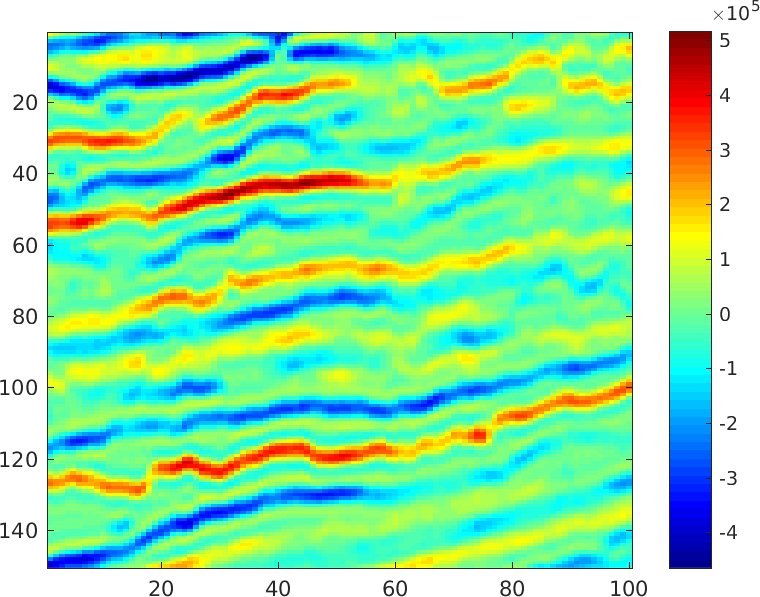
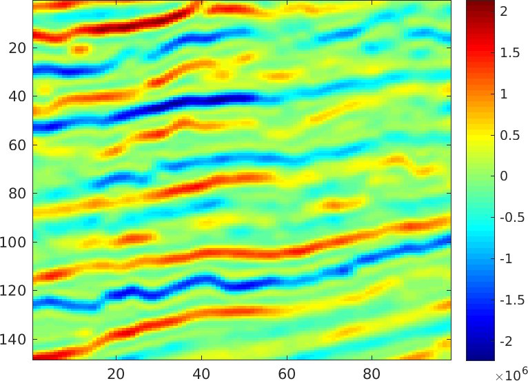
Figure 7. Seismic image (left), and coordinate of filtered feature vector (right).

3.4.2. Diffusion operator eigenfunctions

Next, we define the kernel $W(i,j)$ using the filtered feature vectors and normalized $W(i,j)$ appropriately to define a diffusion operator $P(i,j)$. The first two (nontrivial) eigenvectors of $P$ are are plotted in Figure 8. As expected the first eigenvector is approximately monotone, while the second eigenvector resembles a higher order oscillation. The subsequent eigenvectors additionally contain oscillations in the horizontal direction. Therefore, the underlying domain corresponds to some tall rectangular domain whose height is approximately $2-3$ times its width.

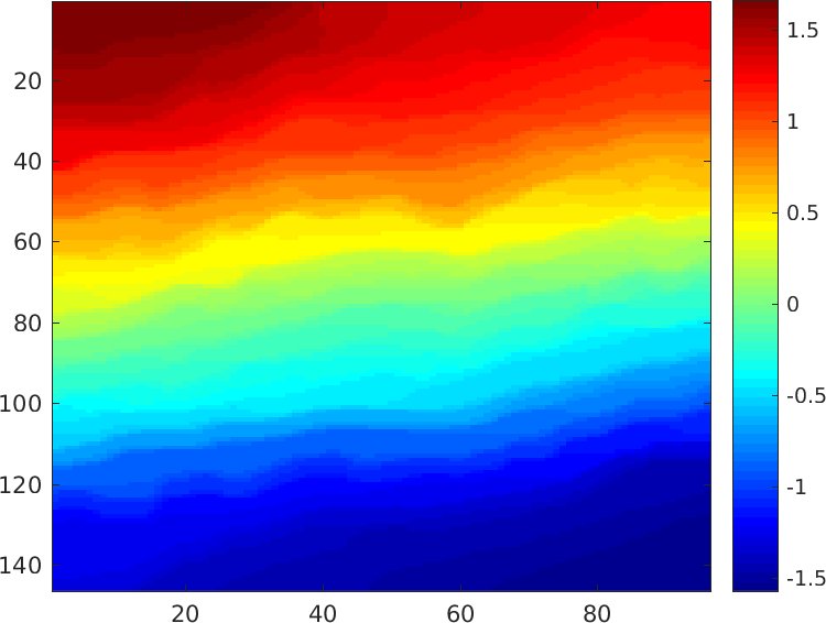
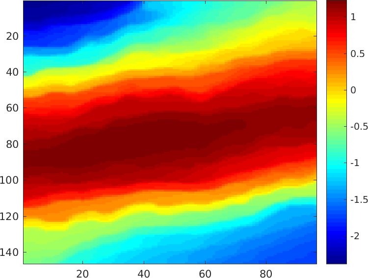
Figure 8. First (left) and second (right) eigenfunction of the diffusion operator $P$.

3.4.3. Flattening

Given the first eigenfunction of the diffusion operator $P$, we can recover the depth function by assuming this eigenfunction coincides with the first Neumann Laplacian eigenfunction on some tall thin rectangle. The result of this flattening procedure is plotted in Figure 9.

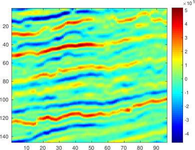
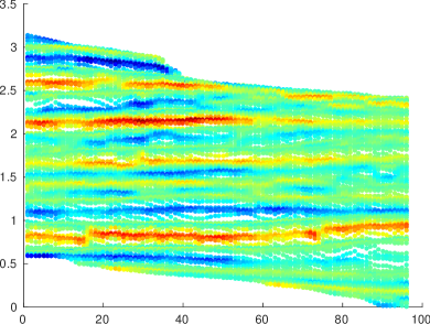
Figure 9. Seismic image (left), and result of diffusion flattening (right).

3.4.4. Magnified flattening

Comparing the scatter plot to the original seismic image in Figure 9 it is evident that the layers are already fairly flat. However, at this resolution, the markers in the scatter plot are overlapping. By zooming into the scatter plot and the corresponding area in the seismic image, we can see that the description generated by the reparameterization is in fact far richer than simply flattening. In Figure 10, we zoom into the interval $[90,130]$ on the $y$-axis of the seismic image in Figure 9, and we zoom into a corresponding interval on the $y$-axis of the reparameterized image. At this new level of zoom white space appears between the scatter plot markers. This white space is simply a result of the markers diminishing in size, and demonstrates that the diffusion flattening procedure offers an advantageous side effect: the points within a layer are automatically clustered when the depth function is reparameterized by the first eigenfunction of the diffusion operator.

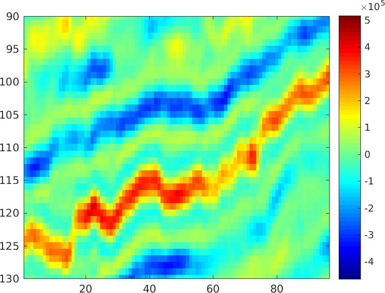
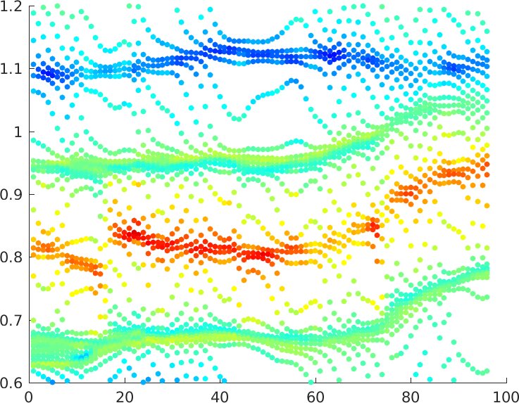
Figure 10. Seismic image with $y$-axis zoomed into $90$ to $130$, and corresponding region of flattened image. At this zoom level, the detailed structure of the diffusion layer organization becomes evident.

3.4.5. Example Summary

Given a two dimensional seismic image we have defined a diffusion process on the image using structural information from the surrounding pixels. This diffusion processes propagates rapidly along the layers of the seismic image and slowly perpendicular to these layers. Therefore, the diffusion corresponds to isotropic diffusion on some underlying domain, roughly shaped like a tall thin rectangle where the layers of the seismic image are roughly horizontal. Therefore, using our intuition backed by Theorem 1.1, we can recover the depth function in the image by assuming the first eigenfunction of the diffusion operator resembles the first Neumann Laplacian eigenfunction on the rectangle.

Appendix A Algorithm details

A.1. Adaptive Filtering

In this section, we describe the adaptive filtering method. The filtering method is described for a general three dimensional image since it requires no additional effort, whereas for the rest of the algorithm we are mainly interested in the filtered feature vectors computed for a two dimensional slice of a three dimensional seismic image. Let $X$ denote a three dimensional seismic image, $i$ denote a pixel from $X$, and $v(i)$ denote the value associated with pixel $i$. Each interior pixel $i$ of the seismic image is surrounded by a $3\times 3\times 3$ cube of pixels in $X$. Given an interior pixel $i$, let $g(i)$ denote the set of values associated with the pixels surrounding $i$. By fixing a method of rearranging a $3\times 3\times 3$ cube of pixels into a vector, we can consider each $g(i)$ as a vector in $\mathbb{R}^{27}$. Given a collection of feature vectors $g(i)$, we apply principal component analysis (PCA) to create a low dimensional description of each $g(i)$. Specifically, let $A$ denote the $27\times N$ matrix whose columns consist of the feature vectors $g(i)$ for each of the $N$ interior pixels. Define the feature covariance matrix

$$C=\frac{1}{1-N}\left(A-A\frac{1}{N}11^{T}\right)\left(A-A\frac{1}{N}11^{T}\right)^{T},$$

where $1$ denotes a column vector of all ones in $\mathbb{R}^{N}$. Let $u_{1}$ denote the principal component of $C$, that is, the eigenvector of $C$ associated with the largest eigenvalue. To each pixel $i$, we associate a scalar value $w(i)$ defined by

$$w(i)=u_{1}^{T}g(i).$$

We refer to $w(i)$ as the filtered pixel value of $i$. Next, we define the filtered feature vector $f(i)$ as the vector in $\mathbb{R}^{27}$ whose entries are the filtered pixel values $w(j)$ of the pixels $j$ in the $3\times 3\times 3$ cube of pixels surrounding pixel $i$. As before, the $3\times 3\times 3$ cubes of pixels are converted into vectors via some fixed method of rearrangement. The filtered features $f(i)$ are used to define the diffusion process in the following section.

Summary of Adaptive Filtering

To each pixel $i$ we associated the cube of surrounding pixel values $g(i)$, and used PCA to summarize each cube by a single coordinate $w(i)$. Finally, we associated each pixel with a filtered feature vector $f(i)$, corresponding to a cube of the surrounding filtered coordinates $w(i)$.

A.2. Kernel Construction

In this section we describe the construction of a diffusion process on the pixels of a seismic image, which propagates rapidly along the layers of the image and slowly perpendicular to these layers. For simplicity we restrict our attention to a two dimensional slice of a three dimensional seismic image, as shown in the left side of Figure 7.

Let $Y$ denote a two dimensional slice of a given three dimensional seismic image, $i$ denote a pixel of $Y$, and $f(i)$ denote the filtered feature vector $f(i)\in\mathbb{R}^{27}$ whose construction is described in the previous section. Let $x(i)$ denote the spatial coordinates of pixel $i$ in $Y$. For example, if $Y$ is of dimension $m\times n$, then $x(i)(x_{1}(i),x_{2}(i))\in\{1,\ldots,m\}\times\{1,\ldots,n\}$. For each pixel $i\in Y$, let $N_{r}(i)$ denote the collection of pixels

$$N_{r}(i)=\{j:\|x(i)-x(j)\|_{2}<r\},$$

where $r>0$ is some small radius, e.g., $r=2$. We will refer to $N_{r}(i)$ as the propagation neighborhood. In addition to $N_{r}(i)$ we define a larger calibration neighborhood $C_{R}(i)$ for $R>r$, which is coarsely sampled. Specifically, if $(x_{1}(i),x_{2}(i))=x(i)$ denotes the spatial coordinates of pixel $i$, then we define

$$C_{R}(i)=\{j:\|x(j)-x(i)\|_{2}<R,x_{1}(j)-x_{1}(i)\equiv 0\,(\text{mod }3),x_{2}(j)-x_{2}(i)\equiv 0\,(\text{mod }3)\},$$

so that $C_{R}(i)$ consists of the pixels whose $3\times 3\times 3$ feature cubes are non-overlapping, and whose spatial distance is less than $R$ from pixel $i$. Using the calibration neighborhood $C_{R}(i)$ we define

$$M(i)=\max_{j\in C_{R}(i)}\|f(i)-f(j)\|_{2}^{2},$$

and define the asymmetric kernel $W_{\varepsilon}(i,j)$ by

$$W_{\varepsilon}(i,j)=\left\{\begin{array}[]{cl}\exp\left(-\frac{\|f(i)-f(j)\|_{2}^{2}}{\varepsilon M(i)}\right)&\text{if}\quad j\in N_{r}(i)\\ 0&\text{if}\quad j\not\in N_{r}(i).\end{array}\right.$$

The purpose of defining the calibration neighborhood $C_{R}(i)$ rather than just normalizing the kernel over $N_{r}(i)$ is to avoid the case where the entire neighborhood $N_{r}(i)$ is contained in a single layer. In this case, all pixels within $N_{r}(i)$ should be strongly connected, but normalizing using $N_{r}(i)$ would emphasize minute differences in the feature vectors. Of course, this problem could be avoided by increasing the radius $r$; however, increasing $r$ increases the number of nonzero entries in each row of the kernel $W$ by a factor of $r^{2}$: better to define a separate calibration neighborhood $C_{R}(i)$ to avoid both the normalization and complexity issues. As defined, the kernel $W_{\varepsilon}(i,j)$ takes a maximum value of $1$ when $f(i)=f(j)$, and a minimum value of

$$W_{\varepsilon}(i,j)=\exp\left(-\frac{1}{\varepsilon}\right)$$

if $\|f(i)-f(j)\|_{2}^{2}=M(i)$. Therefore, rather than choosing $\varepsilon>0$ we parameterize our model by $\delta>0$ and define

$$\varepsilon=-\frac{1}{\log\delta}$$

With this parameterization, the minimum possible value of the kernel in each neighborhood is $\delta$. In order to be compatible with the standard Diffusion Maps framework described in [12], the kernel used to define the diffusion process must be symmetric. Therefore, we define a symmetrized version $K(i,j)$ of $W_{\varepsilon}(i,j)$ by

$$K(i,j)=\frac{1}{2}\left(W_{\varepsilon}(i,j)+W_{\varepsilon}(j,i)\right)$$

Notice that the dependence on $\varepsilon$ of $K$ (which in turn depends on $\delta$) was suppressed for notational simplicity.

Summary of Kernel Construction

We first choose a radius $r>0$ which defines a spatially local propagation neighborhood. Second, we choose a radius $R>0$ which defines a coarse calibration neighborhood. Third, we choose a parameter $\delta>0$, which determines the minimum possible affinity in each neighborhood. Finally, we symmetrize the constructed kernel, resulting in the symmetric kernel $K(i,j)$. In the following section, we use the kernel $K$ in combination with the standard Diffusion Maps framework [12] to create a description of the layer geometry of the image $Y$.

A.3. Layer Organization

In this section, we describe how the kernel $K$ defined in the previous section can be used to generate a description of the layer structure of $Y$. In particular, we use the $(\alpha=0)$ diffusion kernel construction of Diffusion Maps [12] in combination with the randomized matrix decomposition technique as introduced by [13], as well as intuition about the form of the Laplacian-Neumann eigenvectors, to define a new depth function $h$ of the pixels of the seismic image $Y$.

Given the kernel $K(i,j)$, we define the diffusion operator $P$ by

$$P(i,j)=\frac{K(i,j)}{q(i)},$$

where

$$q(i)=\sum_{j}K(i,j).$$

The matrix operator $P(i,j)$ is row stochastic; therefore, $P$ is a Markov operator when applied from the right, and a diffusion or averaging operator when applied from the left. Since $P$ is similar to the symmetric matrix $A$,

$$A=Q^{1/2}PQ^{-1/2},$$

where

$$Q=\operatorname{diag}(q),$$

the matrix $P$ is diagonalizable and has real eigenvalues. Moreover, the eigenvectors $\psi_{j}$ of $P$ are exactly given by

$$\psi_{j}=Q^{-1/2}\phi_{j}$$

where $\phi_{j}$ is an eigenvector of $A$ of the same eigenvalue $\lambda_{j}$.

Therefore, in order to compute the eigenvectors of $P$, it suffices to decompose $A$ and apply $Q^{-1/2}$. From a computational point of view, working with $A$ is preferable since $A$ is symmetric and has operator norm $1$. Furthermore, the operator $A$ is sparse by construction with most $2|N_{r}(i)|$ nonzero entries in each row $i$, and is of finite rank invariant to the sampling density of the data (at least when when the kernel bandwidth is fixed). Therefore, randomized matrix decomposition algorithms, such as described in [14], provide an efficient method to compute the top few eigenvectors of $A$. Given these eigenvectors, the eigenvectors of $P$ can be recovered by applying $Q^{-1/2}$ as previously mentioned.

By construction, the eigenvectors of $P$ approximate the Neumann Laplacian eigenfunctions of the underlying geometry of the pixels of $Y$ on which $P$ corresponds to isotropic diffusion, cf. [12]. The largest eigenvalue $\lambda_{0}$ of $P$ is $1$, which corresponds to a constant eigenvector $\psi_{0}=1$. However, the first nontrivial eigenvector $\psi_{1}$ is of interest. Recall that $P$ is based on the kernel $K$, which is defined to be large (i.e., close to $1$) between similar pixels within a spatial neighborhood, and on the order of a small constant $\delta$ (e.g., $\delta=10^{-7}$) between highly dissimilar pixels with respect to the calibration neighborhood. While moving along a layer in the seismic image $Y$, the pixels (as characterized by the feature vector $f(i)$) should be highly similar. However, when moving perpendicular to a layer, the feature vectors $f(i)$ will change rapidly, and pixels quickly become highly dissimilar to the starting point. As a result, the diffusion described by $P$ travels rapidly along the layers of $Y$, and slowly perpendicular to these layers. That is to say, the underlying geometry of the pixels on which $P$ represents isotropic diffusion must have a relatively small distance between pixels on the same layer when compared to pixels on different layers, which are equally spatially distant in $Y$.

Therefore, the underlying geometry of $P$ roughly corresponds to a tall rectangle shape, that is, a rectangle whose heigh is greater than its width. Of course, due to the variation in the earth, the underlying domain will not be exactly rectangle shaped, but resemble some type of deformed tall rectangle where the layers run horizontally and are relatively flat. In Section 2, we proved an explicit stability result, which indicates that the first Neumann Laplacian eigenfunctions on tall rectangle are highly stable under deformations on the underlying domain. This proof is consistent with numerical experiments. Intuitively, the stability results from the fact that if a rectangles height is a least twice its width, the first couple Neumann Laplacian eigenfunctions will only oscillate vertically, which provides a buffer to any horizontal oscillations.

Recall, that the first Neumann Laplacian eigenfunction on the rectangle $[0,\varepsilon]\times[0,1]$ where $1>\varepsilon>0$ is

$$\psi_{1}(x,y)=\cos(\pi y)$$

Assuming that $\psi_{1}$ is of a similar form, the height function on the underlying domain can be recovered by

$$h(i)=\arccos\left(\frac{\psi_{1}(i)-\min_{j}\psi_{1}(j)}{\max_{j}\psi_{1}(j)-\min_{j}\psi_{1}(j)}\right)$$

up to linear scaling. Depending on the height of the underlying rectangular domain, the next couple eigenfunctions $\psi_{2}$, $\psi_{3}$, etc. should resemble $\cos\pi 2y$, $\cos\pi 3y$, etc., until the first eigenvector emerges with horizontal oscillations, after which the eigenfunctions likely become difficult to interpret because of noise.

Summary of layer organization

We have constructed a diffusion operator $P$ whose eigenfunctions approximate the Neumann Laplacian eigenfunctions on the underlying domain, which by the construction of the kernel $K$ should resemble a tall rectangle. Using randomized matrix decomposition techniques, the eigenfunctions of $P$ can be computed, and the $\arccos$ function can be used to recover the height function of the underlying rectangular domain. This height function should organize the layers of the image.

Acknowledgements

We would like to thank Anthony Vassiliou and Lionel Woog for the seismic data and for bringing the application problem to our attention. Furthermore, we would like to thank Ronald Coifman for numerous insightful conversations, and Stefan Steinerberger for many helpful comments and suggestions.

References

- [1] S. Lafon, Diffusion Maps and Geometric Harmonics. PhD thesis, Yale University, 2004.
- [2] R. R. Lederman and R. Talmon. Common manifold learning using alternating-diffusion. Yale Tech. Rep., 2014.
- [3] R. R. Coifman and M. J. Hirn. Diffusion maps for changing data. Appl. Comput. Harmon. Anal., 36(1):79–107, 2014.
- [4] R. Talmon and R. R. Coifman. Empirical intrinsic geometry for nonlinear modeling and time series filtering. Proc. Natl. Acad. Sci. USA, 110:12535–12540, 2013.
- [5] A. Singer and H. Wu. Vector diffusion maps and the connection laplacian. Comm. Pure Appl. Math, 65(8):1067–1144, 2012.
- [6] A. Schclar, A. Averbuch, N. Rabin, V. Zheludev, and K. Hochman. A diffusion framework for detection of moving vehicles. Digit. Signal Process., 20(1):111–122, 2010.
- [7] L. du Plessis, S. Damelin, and M. Sears. Reducing the dimensionality of hyperspectral data using diffusion maps. Geoscience and Remote Sensing Symposium IEEE International IGARS, 4:885–888, 2009.
- [8] M. Belkin and P. Niyogi. Laplacian eigenmaps for dimensionality reduction and data representation. Neural Comput., 15:1373–1396, 2003.
- [9] J. Lomask. Seismic Volumetric Flattening and Segmentation. PhD thesis, Stanford University, 2007.
- [10] D. Gao. 3d seismic volume visualization and interpretation: An integrated workflow with case studies. Geophysics, 74(1):1–12, 2009.
- [11] D. Parks. Seismic image flattening as a linear inverse problem. Master’s thesis, Colorado School of Mines, 2010.
- [12] R. R. Coifman and S. Lafon. Diffusion maps. Appl. Comput. Harmon. Anal., 21(1):5–30, 2006.
- [13] F. Woolfe, E. Liberty, V. Rokhlin, and M. Tygert. A fast randomized algorithm for the approximation of matrices. Appl. Comput. Harmon. Anal., 25(3):335–366, 2008.
- [14] N. Halko, P.-G. Martinsson, and J. A. Tropp. Finding structure with randomness: Probabilistic algorithms for constructing approximate matrix decompositions. ArXiv e-prints, 2009.