Surface Normals in the Wild

Abstract

We study the problem of single-image depth estimation for images in the wild. We collect human annotated surface normals and use them to train a neural network that directly predicts pixel-wise depth. We propose two novel loss functions for training with surface normal annotations. Experiments on NYU Depth and our own dataset demonstrate that our approach can significantly improve the quality of depth estimation in the wild.

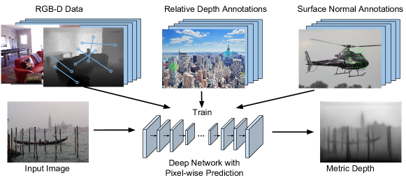
Figure 1: Building on top of the work of Chen et al. [7], we crowdsource annotations of surface normals and use the collected surface normals to help train a better depth prediction network.

1 Introduction

Single-image depth estimation is an important computer vision problem that has the potential to majorly boost higher-level tasks such as object recognition and scene understanding. However, despite extensive research [23, 10, 22, 1, 9, 20, 29, 31, 16, 6, 26, 24, 2], single-image depth estimation remains difficult. In particular, it remains difficult to estimate depth for unconstrained images of arbitrary scenes, because, as prior work [7] has pointed out, existing RGB-D datasets used to train current systems were collected by depth sensors. As a result, they consist of a few specific types of indoor and outdoor scenes. Systems trained on these datasets thus cannot generalize to images “in the wild” of arbitrary scenes and compositions.

Recent work by Chen et al. [7] made an attempt to estimate depth for images “in the wild”: they collected human annotations of relative depth—the depth ordering of two points—for random Internet images and use the annotations to train a deep network that directly predicts metric depth. Chen et al. showed that it is possible to improve depth estimation for images in the wild by using human annotations of depth. In particular, they showed that while it is difficult to obtain absolute metric depth (per-pixel depth values) from humans, it is nonetheless feasible to collect indirect, qualitative depth annotations such as relative depth, and use such annotations to learn to estimate metric depth. This strategy does not rely on depth sensors and can work with arbitrary images; it thus has the potential to significantly advance depth estimation in the wild.

One limitation of the work by Chen et al. [7], however, is that annotations of relative depth do not capture all information that is perceptually important. In particular, relative depth is invariant to monotonic transformations of metric depth, meaning that there can be two scenes that are perceptually very different yet are indistinguishable in terms of relative depth. For example, it is possible to bend, wiggle, or tilt a straight line without affecting relative depth (Fig. 2). In other words, relative depth does not capture important perceptual properties such as continuity, surface orientation, and curvature. As a result, systems trained on relative depth will not necessarily recover depth that is perceptually faithful in all aspects.

In this paper, we build on the work of Chen et al. [7] and address the limitation by introducing an additional type of indirect, qualitative depth annotation—surface normals. Surface carries important information on 3D geometry: they encode the local orientation of surfaces and the derivatives of depth. In fact, given dense surface normals, it is possible to recover full metric depth up to scaling and translation. This suggests that annotations of surface normals can eliminate the ambiguities in relative depth and result in better depth estimation. In addition, it has been well documented in human vision research that humans perceive surface orientation with a remarkable degree of consistency [18]. This suggests that it could be feasible to collect human annotations for images in the wild.

We consider two questions: how to crowdsource annotations of surface normals, and how to use surface normal annotations to help train a network that predicts per-pixel metric depth. To crowdsource surface normals, we develop a UI that allows a user to annotate a surface normal by adjusting a virtual arrow and a virtual tangent plane. This UI allows human annotators to reliably estimate surface normals. With this UI we introduce a dataset called “Surface Normals in the Wild” (SNOW), which consists of surface normal annotations collected from 60,061 Flickr images.

To incorporate surface normal annotations into training, we develop two novel loss functions to train a deep network that directly predicts metric depth. The first loss function is based on directly comparing normals, that is, computing the angular difference between the ground truth normals and the normals derived from the predicted depth. The second loss function is based on comparing depth derivatives, i.e., computing the discrepancy between the derivative of the predicted depth and the derivative given by the ground truth normals. We show that each approach incurs its own trade-offs and emphases on different aspects of depth quality, and should be chosen based on particular applications.

Our main contributions are (1) a new dataset of crowdsourced surface normals for images in the wild and (2) two distinct approaches of for using surface normal annotations to train a deep network that directly predicts per-pixel metric depth. Experiments on both NYU Depth [28] and SNOW demonstrate that surface normal annotations can significantly improve the quality of depth estimation.

Figure 2: Ambiguities of relative depth annotation. Bending, wiggling, or tilting a 3D surface from solid line configuration to dotted line configuration does not change the ordinal relation that point A is farther away from the camera than point B.

2 Related work

Datasets with depth and surface normals Prior works on estimating depth or surface normals have mostly used NYU Depth [28] , Make3D [27], KITTI [13], or ScanNet [8]. Although these datasets provide highly accurate depth, as pointed out by Chen et al. [7] they are limited to specific types of scenes. The same limitation applies to synthetic datasets such as MPI Sintel [5] and the dataset by [25] because the 3D content had to be manually created. The Depth in the Wild (DIW) dataset introduced by Chen et al. [7] takes a major step toward including arbitrary scenes in the wild. However, DIW provides only relative depth annotations, which lack information on many essential 3D properties such as surface normals. We build upon DIW and introduce a new dataset of crowdsourced surface normals for images in the wild.

Open Surfaces [4] is a large dataset of images with annotations of surface properties including surface normals and material. However, open Surfaces is not suitable for depth estimation in the wild: it contains only images of indoor scenes. In addition, it only has surface normals for planar surfaces, whereas our dataset has no such restriction.

Depth and surface normals from a single image There has been a large body of work on estimating depth and/or surface normals from a single image [23, 10, 22, 1, 9, 21, 20, 29, 31, 16, 3]. All these methods use dense ground truth depth or normals during training, except the work of Zoran et al [33] which uses relative depth for training. They all have difficulty generalizing to images in the wild due to the limited scene diversity of the existing datasets that were acquired by depth sensors.

Chen et al. [7] instead use crowdsourced relative depth for training, using indirect depth human annotations to get around the limitations of depth sensors. Our work goes beyond the work of Chen et al. by exploring surface normals.

Two other recent works [12, 32] have also leveraged indirect supervision of depth. In particular, they have used pairs of stereo images to impose constraints on the predicted depth, e.g. the depth estimated from the left image should be consistent with the depth estimated from the right image as dictated by epipolar geometry [12].

Chakrabarti et al. [6] trained a network that simultaneously predicts distributions of depth and distributions of depth derivatives at each pixel location. Then they used a global optimization method to recover a single depth map that is most consistent with the predictions. Our work differs in two ways. First, the only output of our network is a depth map. Our network does not directly predict surface normals or depth derivatives, and thus there is no need for additional optimization steps to harmonizing the outputs. Second, we do not use dense ground truth metric depth in training. Our ground truth annotations are sparse and involve only relative depth and/or surface normals.

Surface normals in 3D reconstruction Surface normals have played important roles in many 3D reconstruction systems. For example, surface normals have been used to infer 3D models [19], create watertight 3D surfaces [17], regularize planar object reconstruction [30], and to aid multi-view reconstruction [11] and structure from motion [15], or depth estimation [14]. In our approach, surface normals are used in training only; the network directly predicts depth, without explicitly producing surface normals.

3 Dataset construction

Similar to the Depth in the Wild (DIW) dataset by Chen et al. [7], we source our images from Flickr using random keywords from an English dictionary. For each image, we extract the focal length of the camera from the EXIF metadata—the focal length is needed for determining the amount of perspective distortion when we visualize a surface normal on top of an image in our UI.

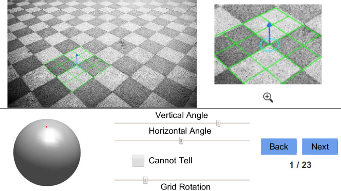
Figure 3: The annotation UI we use for data collection. The query image is displayed on the top left with the keypoint highlighted. A zoom-in view centered at the keypoint is displayed on the top right to help the worker see the details better. Workers then click on the sphere and adjust the slider bars to annotate the surface normal.

To collect surface normal annotations, we present a crowd worker with an image and a highlighted location (Fig. 3). The worker then draws a surface normal using a set of controls: she can pick a point on a sphere, or use two slider bars to adjust the angles (there are two degrees of freedom). The surface normal is visualized as an arrow originating from a 2D grid that represents the tangent plane. Both the arrow and the 2D grid are rendered taking into account the focal length extracted from the image metadata. This visualization is inspired by the gauge figures used in human vision research [18]; it helps the worker perceive the surface normal in 3D.

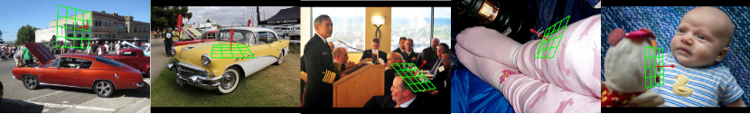
Figure 4: Some examples of the final surface normal annotations we gather for the SNOW dataset. The green grid denotes the tangent plane, and the red arrow denotes the surface normal. For best visual effect, please view in color.

For each image, we pick one random location uniformly from the 2D plane to have its surface normal annotated. Following Chen et al. [7] we only pick one random location to minimize the correlation between annotations.

As the locations are randomly picked, some may fall onto areas where the surface normal is hard to infer, especially when there is a large amount of clutter or texture, e.g. tree leaves in the distance or grass in a field. Surface normals may also be impossible to infer on regions such as the sky or a dark background (some examples are shown in the Appendix). In these cases a user can indicate that the surface normal is hard to tell.

We crowdsource the task through Amazon Mechanical Turk. We randomly inject gold standard samples into the task to identify spammers. Each surface normal is annotated by two different workers. If the two annotations are within 30 degree of each other, then we take the average of the two (renormalized to a unit vector) as the final annotation; otherwise, we discard both annotations.

Fig. 4 shows some examples of the collected normals. In total, we processed 210,000 images on Amazon Mechanical Turk and obtain 60,061 valid samples. On average, it takes about 15 seconds for a worker to annotate one surface normal. The average angular difference between the two accepted annotation is 14.32^∘. This suggests that human annotations usually agree with each other quite well.

3.1 Quality of human annotated surface normals

An important question is how consistent and accurate the human annotations are. To study this, we collect human annotations of surface normals on a random sample of 113 NYU Depth [28] images. Each surface normal is estimated by three human annotators. We compare the human annotations with the ground truth surface normals (derived from the Kinect ground truth depth). We measure the Human-Human Disagreement (HHD) using the average angular difference between a human annotation and the mean of multiple human annotations. We measure Human-Kinect Disagreement (HKD) using the average angular difference between a human annotation and the Kinect ground truth.

We found that the Human-Human Disagreement on our sample is ($7.4^{\circ}$). This suggests that human annotations are remarkably consistent between each other. However, the Human-Kinect Disagreement is $32.8^{\circ}$ which at first glance seems to suggest that human annotations contain a large amount of systemic bias measured against the Kinect ground truth. However, a close inspection reveals that most of the disagreement is a result of imperfect Kinect ground truth rather than biased human estimation.

One source of Kinect error is holes in the raw depth map. Some holes are due to specular or reflective surfaces; others are due to the parallax caused by the RGB camera located slightly away from the depth camera. The holes in the raw Kinect depth map are filled through some heuristic post-processing. Such hole-filling is imperfect. It is especially problematic at cluttered regions because it cannot recover the fine variations of depth and as a result the derived normals will be inaccurate.

Another source of Kinect error is imperfect normals computed from accurate depth. In this experiment we used the official toolkit from the NYU Depth dataset [28] to compute normals. Each normal is computed by fitting a plane to a neighborhood of pixels. But this procedure tends to smooth out normals at or close to sharp normal discontinuities (e.g. at the intersection of two planes or at occlusion boundaries). This problem is especially severe in cluttered regions where there are many such discontinuities. But human estimation of normals is not susceptible to this issue.

We manually inspected every image in our sample and found that 37% of the cases can be attributed to one of the two sources of Kinect error (holes or imperfect normal calculation). Fig. 5 shows examples of such cases. The Human-Kinect disagreement on these problematic cases is 44.32^∘. Excluding these cases, the Human-Kinect disagreement is only 15.64^∘. It is worth noting that in those cases of Human-Kinect disagreement, humans remain remarkably consistent among themselves (average disagreement is 7.17^∘). These results suggest that human annotations of surface normals are of high quality.

It is worth noting that due to the inherent ambiguity of single-image depth estimation, we can never expect humans to match the accuracy of depth sensors, which use more than a single image to recover depth. And in many applications, especially those involving recognition, metric fidelity is not essential. Consistency is the more important quality measure because it means that there is a consistent representation (possibly biased) that we can hope to learn to estimate.

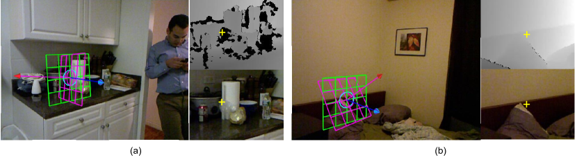
Figure 5: Examples of Kinect error. It shows annotations along with zoom-in views of depth map and RGB image around the keypoint (yellow cross). The red arrow with a purple mesh shows the Kinect ground-truth. Blue arrow and green mesh shows human annotations. (a) lies on a hole in the depth map which is caused by the transparent plastic bag. (b) lies near depth discontinuities. The surface normal in these region cannot be reliably computed.

4 Learning with surface normals

Our goal is to train a deep neural network to perform depth prediction. We build our method upon [7], which uses relative depth as supervision during training. The main idea from  [7] is to train a network using a loss function that penalizes the inconsistency between the predicted depth and the ground truth relative depth (ordinal relations between pairs of points). We propose to incorporate surface normals as additional supervision. This translates to a loss function that encourages the predicted depth to be consistent with both the ground truth relative depth and the ground truth surface normals.

Formally, let $I$ be a training image with $K$ relative depth annotations and $L$ surface normal annotations. Using the same notations of  [7], let $R={(i_{k},j_{k},r_{k})},k=1\dots K$ be the set of relative depth annotations, where $i_{k}$ and $j_{k}$ are the locations of two points in the $k$-th annotation and $r_{k}\in\{>,<,=\}$ is the ground-truth ordinal relation (closer, further, or same distance). Let $S=\{p_{l},n_{l}\}$ be the set of surface normal annotations, where $p_{l}$ is the location of the $l$-th annotation and $n_{l}\in\mathbf{R}^{3}$ is the ground truth surface normal at this location.

We can now express the loss function as follows:

$$L(R,S,z)=\frac{1}{K}\sum_{k=1}^{K}\psi(i_{k},j_{k},r_{k},z)+\lambda\frac{1}{L}\sum_{l=1}^{L}\phi(p_{l},n_{l},z)$$ (1)

where $z$ is the depth map predicted by the network. The loss term $\psi(i_{k},j_{k},r_{k},z)$ measures the inconsistency between the predicted depth map $z$ and the $k$-th relative depth annotation. The loss term $\sum_{l=1}^{L}\phi(p_{l},n_{l},z)$ measures the inconsistency between the predicted depth map $z$ and the $l$-th surface normal annotation. The hyper-parameter $\lambda$ balances the two terms.

A revised relative depth loss Chen et al. [7] define the loss term $\psi(i_{k},j_{k},r_{k},z)$ as

$$\left\{\begin{array}[]{ll}\ln\left(1+\exp(-z_{i_{k}}+z_{j_{k}})\right),&r_{k}\in\{>\}\\ \ln\left(1+\exp(z_{i_{k}}-z_{j_{k}})\right),&r_{k}\in\{<\}\\ (z_{i_{k}}-z_{j_{k}})^{2},&r_{k}\in\{=\}\\ \end{array}\right.$$ (5)

This definition encourages two depth values to be as different as possible if their ground truth ordinal relation is an inequality, or as similar as possible if their ground truth relation is equality. It works well if relative depth is the only form of supervision, as shown by Chen et al. [7], but it is problematic when used in conjunction with annotations of surface normals. The problem is that it encourages the difference of two unequal depth values to be infinitely large. This can potentially conflict with annotations of surface normals, which encourage the depth values to have a specific difference to form a specific surface orientation.

To address this issue we revise the loss term by introducing a margin $\tau>0$ that stops the loss from decreasing if two depth values supposed to be unequal are already at least $\tau$ apart and if two equal depth values supposed to be equal are apart by no more than $\tau$:

$$\left\{\begin{array}[]{ll}\ln\left(1+\exp(-\min(z_{i_{k}}-z_{j_{k}},\tau)\right)),&r_{k}\in\{>\}\\ \ln\left(1+\exp(-\min(z_{j_{k}}-z_{i_{k}},\tau)\right)),&r_{k}\in\{<\}\\ \max(\tau^{2},|z_{i_{k}}-z_{j_{k}}|^{2}),&r_{k}\in\{=\}.\\ \end{array}\right.$$ (9)

To make the loss term compatible with surface normals, we make another modification. We add a softplus transform to the network to enforce positive depth. This is needed because a negative depth means that the object is behind the camera and will cause issues in computing surface normals from the predicted depth.

Angle-based surface normal loss We now consider how to define the loss term $\phi(p_{l},n_{l},z)$ in Eqn. 1 that compares the predicted depth map $z$ with a ground truth surface normal $n_{l}$ at location $p_{l}$.

The first approach we propose is to derive a surface normal $\nu(z)_{p_{l}}$ at the same location from the predicted depth map $z$ and compare the derived normal to the ground truth. Here $\nu$ is a function that maps a depth map to a map of surface normals, and $\nu(z)_{p_{l}}$ is the derived surface normal at location $p_{l}$. The loss term can now be defined as the angular difference between the derived normal and the ground truth normal, expressed as a dot product of the two normals:

$$\begin{split}\phi_{l}(p_{l},n_{l},z)=-<n_{l},\nu(z)_{p_{l}}>.\end{split}$$ (10)

We call this formulation the angle-based surface normal loss.

To derive surface normals from depth, i.e. to implement the function $\nu$, we first back-project the pixels to 3D points in the camera coordinate system, assuming a pinhole camera model with a known focal length $f$. In particular, a pixel located at $(x,y)$ on the image plane with depth $z^{\prime}$ is mapped to the 3D point $(xz^{\prime}/f,yz^{\prime}/f,z^{\prime})$:

$$\beta:(x,y,z^{\prime})\rightarrow(xz^{\prime}/f,yz^{\prime}/f,z^{\prime})$$ (11)

We then compute the surface normal $\nu(z)_{xy}$ for a pixel located at $(x,y)$ using the cross product of the two vectors formed by its adjacent four neighbors (top to bottom, left to right):

$$\begin{split}\nu(z)_{xy}=[\beta(x-1,y,z_{x-1,y})-\beta(x+1,y,z_{x+1,y})]\\ \otimes[\beta(x,y-1,z_{x,y-1})-\beta(x,y+1,z_{x,y+1})],\end{split}$$ (12)

where $\otimes$ denotes cross product and $\beta$ is the back-projection function in Eqn. 11. Combining Eqn. 11, and Eqn. 10 gives a loss term $\phi(p_{l},n_{l},z)$ that is differentiable with respect to the predicted depth $z$ and can be easily incorporated into backpropagation.

Depth-based surface normal loss. The angle-based surface normal loss is natural, and a network trained with this loss in addition to relative depth annotations should predict better depth, as measured by the metric error (comparing the predict depth with ground truth depth in terms of absolute difference). In our experiments, however, we observe that this is not always the case, especially with a large training set. In particular, we observe that a network will predict a depth map that gives better surface normals, but the depth map itself does not improve in terms of metric error.

This leads us to make one theoretical observation. The observation is that when a surface normal is pointing sideways, a small change of the surface normal corresponds to a disproportionally large change in depth values for the neighobring pixels. In other words, metric depth error is very sensitive to the depth values in regions of steep slopes, but the angle-based loss does not reflect this sensitivity (Fig. 6). This could result in the phenomenon that a decrease in the angle-based loss does not corresponds to any notable improvement of metric depth error—the network is not focusing on the steep slopes, the places that would make the most difference in metric depth error.

Figure 6: Two 3D planes (solid line) whose centers have the same distance $d$ to the image plane and whose projections occupy the same amount of area on an image. The predicted surface normals both deviate by $\theta$ from the ground-truth, but incur drastically different metric depth errors $\Delta 1$ and $\Delta 2$.

Based on this observation we propose an alternative loss formulation, which we call depth-based surface normal loss. The idea is to take the predicted depth at a pixel and compute depth value of a neighbor using the ground truth normal. In other words, we compute the depth value the neighbor should take in order to be fully consistent with the ground truth normal. This “should-be” depth is compared with the actual predicted depth for the neighbor, and the difference becomes the penalty in the loss term. This loss is essentially converting a surface normal into the derivative of depth, and then compare it to the actual predicted derivative of depth. This depth-based loss is thus better aligned with metric depth error: surface normal annotations at steep slopes will play a bigger role in the loss.

Specifically, let $p^{T}$, $p^{B}$, $p^{L}$, $p^{R}$ be the top, bottom, left, right neighbors of pixel $p$. We first obtain the back projection $X^{T}$ of $p^{T}$ using the predicted depth $z_{p^{T}}$ (same as in Eqn. 11). Let $\Pi^{T}$ denote the plane that goes through $X^{T}$ and is oriented according to the ground truth normal $n_{p}$. By intersecting $\Pi^{T}$ with a ray that originates from the camera center and goes through the bottom neighbor $p^{T}$ in the image plane, we obtain the “should-be” depth value $\hat{z}_{p^{B}}$ for the bottom neighbor $p^{B}$. Similarly, we can obtain the “should-be” depth value for the top neighbor from the bottom neighbor ($\hat{z}_{p^{T}}$ from $z_{p^{B}}$), for the left neighbor from the right neighbor ($\hat{z}_{p^{L}}$ from $z_{p^{R}}$), and for the right neighbor from the left neighbor ($\hat{z}_{p^{R}}$ from $z_{p^{L}}$). Finally, the loss term is defined as the difference between the “should-be” depth and the actual predicted depth for all neighbors.

$$\phi_{l}(p_{l},n_{l},z)=\sum_{i\in\{T,B,L,R\}}(\hat{z}_{p_{l}^{i}}-z_{p_{l}})^{2}/(\hat{z}_{p_{l}^{i}}+z_{p_{l}})^{2},$$ (13)

which is differentiable with respect to $z$. Note that the squared difference between the two depth values is normalized by their squared sum. This is for scale invariance; otherwise the network will minimize the loss mostly by shrinking the depth values with little regard to the normals.

Multiscale normals In addition to introducing depth-based loss, we consider yet another strategy to address the issue of angle-based surface normal loss. The strategy is to collect surface normal annotations at multiple resolutions. That is, we can collect some surface normal annotations at lower resolutions. The rationale is that the steep slopes get smoothed out in lower resolutions and become less steep, which brings the angle-based loss more in line with metric depth error. To use the normals from lower resolutions, we add downsampling layers to the network to produce depth maps of lower resolutions, and add an angle-based loss at each additional resolution of the depth map.

5 Experiments on NYU Depth

We perform extensive experiments on NYU Depth [28]. The ground truth metric depth available in NYU Depth allows us to simulate and evaluate how adding surface normal annotations as indirect supervision can improve the prediction of metric depth, which is impossible for images in the wild, which do not have metric depth ground truth.

Implementation details For all our experiments on NYU Depth, we use the same network architecture proposed in  [7]. The only difference is two modifications made to ensure that the loss term on relative depth will not encourage the predicted depth to deviate from the true metric depth, thus minimizing conflict with the loss term on surface normals. First, we add a softplus layer to ensure positive depth. Second, we take the log of the predicted depth before sending it to the relative depth loss in Eqn. 9. Taking the difference of the log depth is the same as taking the log of the depth ratio, which is more consistent with the relative depth annotations in NYU Depth [7, 33] because the ground truth ordinal depth relations are based on thresholding depth ratios rather than thresholding depth difference.

For relative depth “annotations” on NYU Depth, we use the same set as in  [7]. For surface normal “annotations”, we generate them from the ground-truth depth using Eq 12. Unless otherwise noted, in all our models trained with surface normals, we provide 5,000 surface normal annotations at random locations per image.

Main experiments We compare 5 models: (1) a model trained with relative depth only (d); (2) a model trained with relative depth and surface normals using the angle-based loss (d_n_al); (3) same as (2) but using surface normals from multiple resolutions while keeping the total number of normal samples the same (d_n_al_M). (4) a model trained with relative depth and surface normals using depth-based loss (d_n_dl). (5) same as (4) but using surface normals from multiple resolutions while keeping the total number the same (d_n_dl_M).

As in prior work [7, 33], for each of the 5 models we train and evaluate on NYU Subset, a standard subset of 1449 images in NYU Depth, and NYU Full, the entire NYU Depth. Models trained on NYU Full are named with a _F suffix). In this section we discuss quantitative results. For qualitative results, please refer to the Appendix.

Evaluating metric depth Metric depth error measures the metric differences between the predicted depth map and the ground-truth depth map. Following prior work [7, 9, 33], we evaluate the root mean squared error (RMSE), the log RMSE, the log scale-invariant RMSE (log RMSE(s.inv)), the absolute relative difference (absrel) and the squared relative difference (sqrrel); their precise definitions can be found in [10]. Because single-image depth has scale ambiguity, before evaluation we normalize each predicted depth map such that it has the same mean and variance as those of the entire training set, as is done in [7].

However, such normalization is too crude in that it forces every predicted depth map to have the same mean and variance regardless of the input scene, which will unfairly penalize accurate predictions for scenes with a different mean and variance. We therefore propose a new error metric Least-Square RMSE (LS-RMSE) that better handles scale ambiguity in evaluation: for a predicted depth map $z$ and its ground-truth $z^{*}$ with pixels indexed by i, we compute the smallest possible sum of their squared differences under a global scaling and translation of the depth values:

$$\mathrm{LS\_RMSE}(z,z^{*})=\min_{a,b}\sum_{i}(az_{i}+b-z^{*}_{i})^{2}.$$ (14)

Note that computing this error metric is the same as finding the least square solution to a system of linear equations, which has a well-known closed form solution.

Tab. 1 reports the results on metric depth error. We can see that our baseline model trained with relatived depth only matches or exceeds the metric depth error reported by Chen et al. [7]. We attribute this improvement to our revised relative depth loss (Eqn. 9), which does not encourage exaggerating depth differences once the ordering is correct.

On both NYU Subset and NYU Full, adding surface normals in training achieves significant improvement in metric depth quality, as reflected most notably in LS-RMSE. The improvement in metrics other than LS-RMSE is less significant, indicating a mismatch of depth scale. Among the models trained with surface normals, the one trained with the depth-based loss (d_n_dl_F) performs the best, as expected from our discussion in Sec. 4. On NYU Full, it outperforms the relative-depth-only baseline significantly on LS RMSE, approaching the models trained with full ground truth metric depth maps (Eigen(V) [9], Chakrabarti [6]).

The model trained with the angle-based normal loss yields no improvemet on NYU Subset and negative improvement on NYU Full, which can be explained by our theoretical observation that the angle-based loss is misaligned with the metric depth error. The misalignment is especially notable on a bigger dataset, which is harder to fit and can cause the network to “give up” on the steep slopes, which account for very little in the angle-based normal loss. Using multiscale normals helps as expected, but it is not enough to overcome the misalignment on NYU Full to outperform the relative-depth-only baseline.

Evaluating relative depth We also evaluate a predicted depth map on ordinal error: disagreement with ground truth ordinal relations between selected locations. We use the same set of ground truth ordinal relations from  [7], and report the same metrics: WKDR, the weighted disagreement rate between the predicted ordinal relations and the ground-truth ordinal relations, and its variants WKDR⁼ (WKDR of pairs whose ground-truth order is =) and WKDR^≠(WKDR of pairs whose ground-truth order is either $>$ or $<$).

Following  [7], we predict the ordinal relation of point A and B by thresholding on difference of the predicted depth.

The results on relative depth are shown in Tab. 2. First it is interesting to observe that our relative-depth-only baseline model is slightly worse than Chen et al. [7], which also trains with only relative depth. We attribute this difference to our revised relative depth loss (Eqn. 9)—the loss in Chen et al. [7] encourages exaggerating depth differences, which leads to better relative depth performance at the expense of metric accuracy, as reflected by Tab. 1.

Interestingly, adding normals improves ordinal error, but only from the angle-based normal loss, not from the depth-based normal loss. This is because depth-based normal loss places great emphasis on getting the exact steep slopes, but this does not make any difference to ordinal error as long as the sign of the slope is correct.

Training	Method	RMSE	RMSE	log RMSE	absrel	sqrrel	LS
Data			(log)	(s.inv)			RMSE
NYU	d	1.12	0.39	0.26	0.36	0.45	0.64
Subset	d_n_al	1.13	0.39	0.26	0.36	0.45	0.65
	d_n_al_M	1.11	0.39	0.25	0.36	0.44	0.59
	d_n_dl	1.11	0.39	0.25	0.35	0.44	0.58
	d_n_dl_M	1.11	0.39	0.25	0.36	0.45	0.59
	Chen [7]	1.12	0.39	0.26	0.36	0.46	0.65
	Zoran [33]	1.20	0.42	-	0.40	0.54	-
NYU	d_F	1.08	0.37	0.23	0.34	0.41	0.52
Full	d_n_al_F	1.09	0.38	0.24	0.34	0.42	0.55
	d_n_al_F_M	1.09	0.38	0.23	0.34	0.41	0.53
	d_n_dl_F	1.08	0.37	0.23	0.34	0.41	0.50
	d_n_dl_F_M	1.09	0.38	0.24	0.35	0.43	0.52
	Chen_Full [7]	1.09	0.38	0.24	0.34	0.42	0.58
	Eigen(V)* [9]	0.64	0.21	0.17	0.16	0.12	0.47
	Chakrabarti* [6]	0.64	0.21	0.17	0.15	0.12	0.47

Table 1: Metric depth error evaluated on the NYU Depth dataset. Models with a * suffix are trained on full metric depth.

Training	Method	WKDR	$\text{WKDR}^{=}$	$\text{WKDR}^{\neq}$
Data
NYU	d	37.6%	36.4%	39.3%
Subset	d_n_al	36.5%	35.5%	37.9%
	d_n_al_M	34.6%	33.4%	36.3%
	d_n_dl	38.7%	36.9%	40.5%
	d_n_dl_M	39.0%	37.7%	40.5%
	Chen [7]	35.6%	36.1%	36.5%
	Zoran [33]	43.5%	44.2%	41.4%
NYU	d_F	29.2%	32.5%	28.0%
Full	d_n_al_F	27.6%	31.5%	26.6%
	d_n_al_F_M	27.9%	32.2%	26.6%
	d_n_dl_F	30.9%	31.7%	31.4%
	d_n_dl_F_M	35.5%	38.9%	34.6%
	Chen_Full [7]	28.3%	30.6%	28.6%
	Eigen(V)* [9]	34.0%	43.3%	29.6%
	Chakrabarti* [6]	27.5%	30.0%	27.5%

Table 2: Ordinal error evaluated on the NYU Depth dataset. Models with a * suffix are trained on full metric depth.

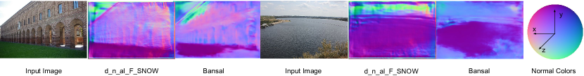
Figure 7: Normal maps produced by our model and Bansal [2]. Please view in color. More examples are in the Appendix.

Evaluating surface normals We now evaluate the predicted depth in terms of surface normals derived from it. We use the same metrics as in [9]: the mean and median of angular difference with the ground-truth, and the percentages of predicted samples whose angular difference with the ground-truth are under a certain threshold. The ground truth normals for test are from NYU Depth toolkit [28], as is done in [31, 9]. We also evaluate the derived surface normals from other depth-estimation models, including (1) state-of-the-art depth estimation method of Eigen [9] and Chakrabarti [6]; (2) The original method of Chen et al. [7] augmented with a softplus layer to ensure positive depth but otherwise trained the same way with relative depth only (Chen* and Chen_Full*).

We report the results in Tab. 3. As expected, models trained with the angle-based normal loss perform better than any other models in terms of surface normals derived from depth, as the loss directly targes the normal error metric.

For reference, we also evaluate state of art methods that directly predict surface normals: Bansal [2], Eigen [9] and Wang [31]. Note that these models are trained on the full dense normal maps on NYU Full whereas our models are trained with only a sparse set of normals. Yet our best model (d_n_al_F) outperforms Wang [31].

Training	Method	Angle Distance		% Within $t^{\circ}$
Data		Mean	Median	11.25∘	22.5∘	30∘
NYU	d	45.46	40.62	7.56	23.65	35.10
Subset	d_n_al	37.53	31.93	13.04	34.38	47.39
	d_n_al_M	35.39	29.51	15.50	38.43	51.40
	d_n_dl	40.53	34.58	11.40	31.13	43.56
	d_n_dl_M	41.88	35.76	10.73	29.69	41.88
	Chen* [7]	50.68	44.96	4.16	16.77	28.21
NYU	d_F	29.45	22.71	22.31	50.71	63.65
Full	d_n_al_F	25.92	20.09	26.28	56.45	69.26
	d_n_al_F_M	26.50	20.42	26.41	55.47	68.09
	d_n_dl_F	30.85	24.51	24.51	46.93	60.31
	d_n_dl_F_M	37.63	31.58	13.41	34.97	47.97
	Chen_Full* [7]	30.35	24.37	18.64	46.80	61.42
	Eigen(V) [9]	35.97	28.34	17.67	41.12	53.49
	Chakrabarti [6]	29.80	20.43	31.34	54.90	64.57
	Wang§ [31]	28.8	17.9	35.2	57.1	65.5
	Eigen(V)§ [9]	22.89	16.26	38.23	63.30	73.18
	Bansal§ [2]	22.63	15.78	39.17	64.17	73.77

Table 3: Surface normals error evaluated on the NYU Depth dataset. The lower the better for Angle Distance metrics. The higher the better for the Percentage within $t^{\circ}$ metrics. Models with a § suffix directly predict surface normals.

Discussion Our expriements on NYU Depth show that surface normal annotations can help depth estimation in the absence of ground truth depth. We have proposed two different surface normal losses. Each has a different set of trade-offs and is appropriate in different applications. If metric fidelity is important, especially at depth discontinuities, then the depth-based loss is more appropriate. If surface orientation is important than the fidelity of depth discontinuities, then the angle-based loss is more appropriate.

	Model	Angle Distance		Within $t^{\circ}$
		Mean	Median	11.25∘	22.5∘	30∘
Normals	d_n_al_F	32.53	27.44	15.40	40.52	54.12
from	d_n_al_F_SNOW	25.75	21.26	21.66	52.98	67.88
Predicted	Chen_Full [7]	35.16	30.26	13.70	36.56	49.56
Depth	Eigen(V) [9]	48.71	46.15	6.35	18.91	28.45
	FCRN [21]	48.74	45.38	5.84	18.29	28.25
Directly	Ours_NYU§	31.96	26.03	18.16	43.72	56.03
Predicted	Ours_NYU_SNOW§	23.33	17.99	30.42	60.54	72.74
Normals	Eigen(V)§ [9]	28.71	23.16	20.98	48.78	61.84
	Bansal§ [2]	27.85	22.25	23.41	50.54	64.09

Table 4: Surface normals error evaluated on SNOW. Models with a § suffix directly predict surface normals.

6 Experiments on SNOW

Since SNOW provides no ground truth of metric depth, it is infeasible to evaluate how training with surface normals helps predict metric depth. We thus evaluate surface normals as an indirect indicator of depth quality for images in the wild. We split SNOW into 10,256 test images and 49,805 training images.

We first evaluate the surface normals derived from depth prediction. Our baselines include state-of-the-art depth estimation methods Eigen [9] and FCRN [21], both trained with full metric depth from NYU Full. We compare these baselines with the d_n_al_F network, our best performing model in terms of normal error. We also fine tune the d_n_al_F network on SNOW (d_n_al_F_SNOW).

We can see in Tab. 4 that our network trained only on NYU Full (d_n_al_F) already outperforms the baselines. Fine-tuning on SNOW yields a significant improvement.

SNOW also enables us to evaluate on methods that directly predict surface normals. We include four models: (1) state-of-the-art surface normal estimation methods of Bansal [2] and Eigen [9]; (2) Chen et al. [7]’s network trained to directly predict normals (Ours_NYU§); (3) Ours_NYU§ fine-tuned on SNOW (Ours_NYU_SNOW§). We can see from Tab. 4 that fine-tuning on SNOW significantly improves surface normal prediction. Finally, Fig. 7 shows examples of qualitative improvement achieved by our network on images in the wild.

7 Conclusion

We have proposed two distinct approaches for using surface normal annotations to train a deep network that directly predicts per-pixel metric depth. We have also introduced a new dataset of crowdsourced surface normals for images in the wild (SNOW). Experiments show that surface normal annotations can advance depth estimation in the wild.

Acknowledgments This work is partially supported by the National Science Foundation under Grant No. 1617767.

See pages 1- of pg_0001.pdf See pages 1- of pg_0002.pdf

References

- [1] M. H. Baig and L. Torresani. Coupled depth learning. arXiv preprint arXiv:1501.04537, 2015.
- [2] A. Bansal, B. Russell, and A. Gupta. Marr revisited: 2d-3d alignment via surface normal prediction. In Proceedings of the IEEE Conference on Computer Vision and Pattern Recognition, pages 5965–5974, 2016.
- [3] J. T. Barron and J. Malik. Shape, illumination, and reflectance from shading. TPAMI, 2015.
- [4] S. Bell, P. Upchurch, N. Snavely, and K. Bala. OpenSurfaces: A richly annotated catalog of surface appearance. ACM Trans. on Graphics (SIGGRAPH), 32(4), 2013.
- [5] D. J. Butler, J. Wulff, G. B. Stanley, and M. J. Black. A naturalistic open source movie for optical flow evaluation. In ECCV, Part IV, LNCS 7577, pages 611–625. Springer-Verlag, Oct. 2012.
- [6] A. Chakrabarti, J. Shao, and G. Shakhnarovich. Depth from a single image by harmonizing overcomplete local network predictions. In Advances in Neural Information Processing Systems, pages 2658–2666, 2016.
- [7] W. Chen, Z. Fu, D. Yang, and J. Deng. Single-image depth perception in the wild. In Advances in Neural Information Processing Systems, pages 730–738, 2016.
- [8] A. Dai, A. X. Chang, M. Savva, M. Halber, T. Funkhouser, and M. Nießner. Scannet: Richly-annotated 3d reconstructions of indoor scenes. arXiv preprint arXiv:1702.04405, 2017.
- [9] D. Eigen and R. Fergus. Predicting depth, surface normals and semantic labels with a common multi-scale convolutional architecture. In ICCV, 2015.
- [10] D. Eigen, C. Puhrsch, and R. Fergus. Depth map prediction from a single image using a multi-scale deep network. In NIPS, 2014.
- [11] S. Galliani and K. Schindler. Just look at the image: viewpoint-specific surface normal prediction for improved multi-view reconstruction. 2016.
- [12] R. Garg, G. Carneiro, and I. Reid. Unsupervised cnn for single view depth estimation: Geometry to the rescue. In European Conference on Computer Vision, pages 740–756. Springer, 2016.
- [13] A. Geiger, P. Lenz, C. Stiller, and R. Urtasun. Vision meets robotics: The kitti dataset. The International Journal of Robotics Research, page 0278364913491297, 2013.
- [14] C. Hane, L. Ladicky, and M. Pollefeys. Direction matters: Depth estimation with a surface normal classifier. In Proceedings of the IEEE Conference on Computer Vision and Pattern Recognition, pages 381–389, 2015.
- [15] S. Ikehata, I. Boyadzhiev, Q. Shan, and Y. Furukawa. Panoramic structure from motion via geometric relationship detection. arXiv preprint arXiv:1612.01256, 2016.
- [16] K. Karsch, C. Liu, and S. B. Kang. Depthtransfer: Depth extraction from video using non-parametric sampling. TPAMI, 2014.
- [17] M. Kazhdan, M. Bolitho, and H. Hoppe. Poisson surface reconstruction. SGP. Eurographics Association, 2006.
- [18] J. J. Koenderink, A. J. Van Doorn, and A. M. Kappers. Surface perception in pictures. Attention, Perception, & Psychophysics, 52(5):487–496, 1992.
- [19] A. Kushal and S. M. Seitz. Single view reconstruction of piecewise swept surfaces. In 2013 International Conference on 3D Vision-3DV 2013, pages 239–246. IEEE, 2013.
- [20] L. Ladicky, J. Shi, and M. Pollefeys. Pulling things out of perspective. In CVPR, 2014.
- [21] I. Laina, C. Rupprecht, V. Belagiannis, F. Tombari, and N. Navab. Deeper depth prediction with fully convolutional residual networks. In 3D Vision (3DV), 2016 Fourth International Conference on, pages 239–248. IEEE, 2016.
- [22] B. Li, C. Shen, Y. Dai, A. van den Hengel, and M. He. Depth and surface normal estimation from monocular images using regression on deep features and hierarchical crfs. In CVPR, 2015.
- [23] F. Liu, C. Shen, and G. Lin. Deep convolutional neural fields for depth estimation from a single image. In CVPR, 2015.
- [24] R. Ranftl, V. Vineet, Q. Chen, and V. Koltun. Dense monocular depth estimation in complex dynamic scenes. In CVPR, 2016.
- [25] S. R. Richter, V. Vineet, S. Roth, and V. Koltun. Playing for data: Ground truth from computer games. In European Conference on Computer Vision, pages 102–118. Springer, 2016.
- [26] A. Roy and S. Todorovic. Monocular depth estimation using neural regression forest. In CVPR, 2016.
- [27] A. Saxena, S. H. Chung, and A. Y. Ng. 3-d depth reconstruction from a single still image. International journal of computer vision, 76(1):53–69, 2008.
- [28] N. Silberman, D. Hoiem, P. Kohli, and R. Fergus. Indoor segmentation and support inference from rgbd images. In ECCV. Springer, 2012.
- [29] P. Wang, X. Shen, Z. Lin, S. Cohen, B. Price, and A. Yuille. Towards unified depth and semantic prediction from a single image. In CVPR. IEEE, 2015.
- [30] P. Wang, X. Shen, B. Russell, S. Cohen, B. Price, and A. L. Yuille. Surge: Surface regularized geometry estimation from a single image. In Advances in Neural Information Processing Systems, pages 172–180, 2016.
- [31] X. Wang, D. Fouhey, and A. Gupta. Designing deep networks for surface normal estimation. In Proceedings of the IEEE Conference on Computer Vision and Pattern Recognition, pages 539–547, 2015.
- [32] J. Xie, R. Girshick, and A. Farhadi. Deep3d: Fully automatic 2d-to-3d video conversion with deep convolutional neural networks. In European Conference on Computer Vision, pages 842–857. Springer, 2016.
- [33] D. Zoran, P. Isola, D. Krishnan, and W. T. Freeman. Learning ordinal relationships for mid-level vision. In ICCV, 2015.