Largest eigenvalues of sparse inhomogeneous Erdős-Rényi graphs

Abstract

We consider inhomogeneous Erdős-Rényi graphs. We suppose that the maximal mean degree $d$ satisfies $d\ll\log n$. We characterize the asymptotic behavior of the $n^{1-o(1)}$ largest eigenvalues of the adjacency matrix and its centred version. We prove that these extreme eigenvalues are governed at first order by the largest degrees and, for the adjacency matrix, by the nonzero eigenvalues of the expectation matrix. Our results show that the extreme eigenvalues exhibit a novel behaviour which in particular rules out their convergence to a nondegenerate point process. Together with the companion paper FBGCBAK2016 , where we analyse the extreme eigenvalues in the complementary regime $d\gg\log n$, this establishes a crossover in the behaviour of the extreme eigenvalues around $d\sim\log n$. Our proof relies on a new tail estimate for the Poisson approximation of an inhomogeneous sum of independent Bernoulli random variables, as well as on an estimate on the operator norm of a pruned graph due to Le, Levina, and Vershynin from LeVershynin .

1 Introduction

The purpose of the present text is to understand the extreme eigenvalues of the adjacency matrix of an inhomogeneous Erdős-Rényi random graph on $n$ vertices in the regime where the maximal mean degree $d$ satisfies $d\ll\log n$. Heuristically, such eigenvalues arise from three different origins: (i) the edge of the limiting bulk eigenvalue density, (ii) vertices of large degrees, and (iii) outliers associated with nonzero eigenvalues of the expectation matrix. One goal of this paper is a precise understanding of this interplay between random matrices on the one hand and the geometry of random graphs on the other. Such questions have several motivations from applications, such as the estimation of the spectral gap and spectral clustering.

The simplest random graph is the Erdős-Rényi random graph $G(n,d/n)$, where each edge is present independently with probability $d/n$. In this case it is rather well understood that the behaviour of the extreme eigenvalues in the regime $d\gg\log n$ is governed by random matrix behavior; see KF ; VuLargestEig ; MR2155709 ; FBGCBAK2016 ; LS1 ; EKYY1 ; EKYY2 . In the complementary regime $d\ll\log n$, the main result available up to now was due to Sudakov and Krivelevich MR1967486 , who showed that the largest eigenvalue of the adjacency matrix is asymptotically equivalent to the maximum of the maximal mean degree $d$ and the square root of the largest degree (their result holds in fact for all regimes of $d$).

Our main result is a description of the behaviour of the $n^{1-o(1)}$ largest and smallest eigenvalues of the adjacency matrix $A$ and its centred version $\underline{A}\!\,\mathrel{\vbox{\hbox{.}\hbox{.}}}=A-\mathbb{E}A$, for an inhomogeneous Erdős-Rényi random graph whose mean degree $d$ is much smaller than $\log n$. Informally, we prove that the $k$-th largest eigenvalue eigenvalue of $\underline{A}\!\,$ satisfies

$$\lambda_{k}(\underline{A}\!\,)\approx\sqrt{\frac{(\log(n/k)}{\log((\log n)/d)}}\,,\qquad k\geqslant n^{1-\varepsilon}\,,\qquad\varepsilon\in(0,1)\,.$$ (1.1)

Under mild additional assumptions (satisfied for instance by stochastic block models), we show that the same result holds for the eigenvalues of $A$, with the exception of some outlier eigenvalues whose locations we also characterize.

A consequence of our results, combined with those from the companion paper FBGCBAK2016 , where we analyse the extreme eigenvalues in the complementary regime $d\gg\log n$, is a crossover in the behaviour of the extreme eigenvalues around $d\sim\log n$ (the same threshold as for the graph connectivity). Indeed, in FBGCBAK2016 we prove that if $d\gg\log n$ then all eigenvalues are asymptotically contained within the support of the semicircle law describing the macroscopic eigenvalue density, while in the current paper we establish for $d\ll\log n$ a novel behaviour of the extreme eigenvalues, which implies that $n^{1-o(1)}$ eigenvalues escape the support of the semicircle law. Their locations are governed by (1.1) and define a distribution that is illustrated in Figure LABEL:Fig:histo_edge below.

It is helpful to analyse the behaviour of the extreme eigenvalues for $d\ll\log n$ in the context of random matrix theory. Until now, in random matrix theory two different types of universal behaviour at leading order of the extreme eigenvalues have been established, exhibited for instance by light- and heavy-tailed Wigner matrices respectively. After a suitable deterministic rescaling of the matrix, these two classes may be characterized as follows.

• The extreme eigenvalues converge to the edge of the support of the asymptotic bulk spectrum.

• The extreme eigenvalues form asymptotically a Poisson point process.

For example, it is known ABP ; SoshPoi ; YL that a Wigner matrix whose entries have tail decay $x^{-\alpha}$ belongs to class (a) if $\alpha>4$ and to class (b) if $\alpha<4$. Moreover, as stated above, in the companion paper FBGCBAK2016 we prove that the Erdős-Rényi graph belongs to class (a) if $d\gg\log n$. Also, sparse heavy-tailed random matrices exhibit a transition between these classes depending on the sparsity and the tail decay of the entries BGPech .

A consequence of our results is that, perhaps surprisingly, for $d\ll\log n$, the (possibly inhomogeneous) Erdős-Rényi graph belongs to neither class (a) nor class (b). Instead, the behaviour from (1.1) results in a sharp increase in the density of eigenvalues as one moves towards the centre of the spectrum, which implies that, no matter the rescaling of the spectrum, any nondegenerate limiting point process will be infinite on compact sets.

The proof consists of two main steps. In a first step, we analyse the distribution of the $n^{1-o(1)}$ largest degrees, and prove that the corresponding vertices are with high probability separated by distance at least 3 from each other. The key tool behind this step is a new sharp estimate (Theorem 3.1 below) on the tail of a sum of inhomogeneous independent Bernoulli random variables. This estimate may be regarded as an improvement for the tails of the well-known Poisson approximation provided by Le Cam’s inequality BHJBook . It is of independent interest. In a second step, we compare the $n^{1-o(1)}$ largest eigenvalues of the graph with those of the graph obtained by only keeping the edges incident to the $n^{1-o(1)}$ vertices of largest degree. The latter corresponds to a block-diagonal matrix whose blocks are associated with star graphs of high central degree. This comparison is based on a sharp estimate on the operator norm of the complementary graph due to Le, Levina, and Vershynin (LeVershynin, , Theorem 2.1).

This text is organized as follows. In the remainder of the introduction, we state our main results, which are proved in Section 2. In Section 3 we state and prove the new tail estimate for Poisson approximation mentioned above.

Notation

The eigenvalues of a Hermitian $n\times n$ matrix $H$ are denoted by $\lambda_{1}(H)\geqslant\lambda_{2}(H)\geqslant\cdots\geqslant\lambda_{n}(H)$. Its operator norm is given by $\|H\|=\max(\lambda_{1}(H),\lambda_{1}(-H))$. For $p\in[0,1]$, we denote by $\mathrm{B}(p)$ the Bernoulli law with parameter $p$, i.e. $\mathrm{B}(p)=(1-p)\delta_{0}+p\delta_{1}$. We denote by $\mathrm{Bin}(p_{1},\ldots,p_{n})$ the law $\mathrm{B}(p_{1})*\cdots*\mathrm{B}(p_{n})$. In particular, $\mathrm{Bin}(p,\ldots,p)$ is the Binomial distribution with parameters $(n,p)$. For $x>0$ use the abbreviation $[x]\mathrel{\vbox{\hbox{.}\hbox{.}}}=\{1,2,\dots,\lfloor{x}\rfloor\}$.

1.1.  Hypotheses and definitions

Throughout this paper, $A$ is the adjacency matrix of an inhomogeneous (undirected) Erdős-Rényi random graph $G$ with vertex set $[n]$, where the edge $\{i,j\}$ is included with probability $p_{ij}\in[0,1]$ independently of the others. Note that we allow loops: there is a loop at vertex $i$ with probability $p_{ii}$.

The maximal edge probability is

$$p_{\max}\mathrel{\vbox{\hbox{.}\hbox{.}}}=\max_{i\neq j}p_{ij}\,.$$

The mean degree of the vertex $i\in[n]$ and the maximal mean degree are defined as

$$d_{i}\mathrel{\vbox{\hbox{.}\hbox{.}}}=\sum_{j}p_{ij}\,,\qquad d\mathrel{\vbox{\hbox{.}\hbox{.}}}=\max_{i}d_{i}$$

respectively.

We always suppose that there are $\kappa>0$ and $\eta\in(0,1)$ such that

$$\la{eq:ordersA}\kappa\leqslant d\leqslant\eta\log n\qquad\and\qquad p_{\max}\leqslant n^{-1+\eta}\,.$$ (1.2)

As all of our error term controls will be uniform, with quantitative rates of convergence, in the parameters $(p_{ij})_{i,j\in[n]}$ such that (LABEL:eq:ordersA) holds, we introduce the following definitions.

Definition 1.1.

≲def:error_control

1. An admissible error function is a function $\psi(n,\kappa,\eta)$ satisfying

   $$\la{def:03041718h49}\forall\kappa>0\,,\qquad\lim_{\begin{subarray}{c}n\to\infty\\ \eta\to 0\end{subarray}}\psi(n,\kappa,\eta)=0\,.$$ (1.3)

2. Given an event $E$ and a condition $\mathcal{A}$ on the parameters $\kappa,\eta,(p_{ij})_{i,j\in[n]}$, we say that, under $\mathcal{A}$, $E$ holds with high probability (w.h.p.) if there is an admissible error function $\psi(n,\kappa,\eta)$ such that

   $$\mathbb{P}(E)\geqslant 1-\psi(n,\kappa,\eta)$$

   for all $\kappa,\eta,(p_{ij})_{i,j\in[n]}$ satisfying $\mathcal{A}$.

3. Given a condition $\mathcal{A}$ on the parameters $\kappa,\eta,(p_{ij})_{i,j\in[n]}$, for two families of random variables $(u_{t}),(v_{t})$ we say that under $\mathcal{A}$, for all $t$, $u_{t}\sim v_{t}$ if there is an admissible error function $\psi(n,\kappa,\eta)$ such that

   $$\mathbb{P}\left(\biggl{\lvert}\frac{v_{t}}{u_{t}}-1\biggr{\rvert}\leqslant\psi(n,\kappa,\eta)\text{ for all }t\right)\geqslant 1-\psi(n,\kappa,\eta)$$

   for all $\kappa,\eta,(p_{ij})_{i,j\in[n]}$ satisfying $\mathcal{A}$.

Let us emphasize that the point in this definition is the uniformity of the error terms in the asymptotic regime where $n\to\infty$, $d=o(\log n)$, and $p_{\max}=n^{-1+o(1)}$. To simplify presentation, in the following we shall not identify the error functions $\psi(n,\kappa,\eta)$ explicitly, although a careful look at our proofs will easily yield explicit expressions for them.

Finally, for $k\in[n]$ we set

$$L_{k}\mathrel{\vbox{\hbox{.}\hbox{.}}}=\frac{\log(n/k)}{\log((\log n)/d)}\,.$$ (1.4)

1.2.  Relation between the centred adjacency matrix and the largest degrees

For $i\in[n]$, let $D_{i}$ denote the degree of the vertex $i$ in the graph $G$. Denote by

$$D_{1}^{\downarrow}\geqslant\cdots\geqslant D_{n}^{\downarrow}$$

the decreasingly ordered degrees $D_{1},\dots,D_{n}$. We also introduce the centred adjacency matrix

$$\underline{A}\mathrel{\vbox{\hbox{.}\hbox{.}}}=A-\mathbb{E}A\,.$$

By definition, $(\mathbb{E}A)_{ij}=p_{ij}$. The following theorem relates the largest eigenvalues of $\underline{A}$ to the largest degrees, whose behaviour is described in Propositions LABEL:propo_position_degree_max and LABEL:27516 below.

Theorem 1.2.

≲thalphall12For any $\varepsilon\in(0,1)$, under (LABEL:eq:ordersA), w.h.p.,

$$\la{Estlam816}\max_{k\in[n^{1-\varepsilon}]}\Bigl{\lvert}\lambda_{k}(\underline{A})-\sqrt{D_{k}^{\downarrow}}\Bigr{\rvert} \leqslant C\sqrt{np_{\max}}+\varepsilon\sqrt{L_{1}}\,,$$ (1.5)

$$\la{Estlam8160}\max_{k\in[n^{1-\varepsilon}]}\Bigl{\lvert}\lambda_{n+1-k}(\underline{A})+\sqrt{D_{k}^{\downarrow}}\Bigr{\rvert} \leqslant C\sqrt{np_{\max}}+\varepsilon\sqrt{L_{1}}\,,$$ (1.6)

where $C$ is a universal constant and $L_{1}$ is defined in (1.4).

The proof of Theorem LABEL:thalphall12 is based on an analysis of the graph spanned by the largest degree vertices, and on (LeVershynin, , Theorem 2.1) due to Le, Levina, and Vershynin on the operator norm of the centred adjacency matrix where all large degree vertices have been removed. The term $\pm\sqrt{D_{k}^{\downarrow}}$ arises as an eigenvalue of a star graph with central degree $D_{k}^{\downarrow}-O(1)$ (see Definition 2.6 below).

By Proposition LABEL:propo_position_degree_max below, for any $\varepsilon\in(0,1)$, we have $D_{1}^{\downarrow}\leqslant(1+\varepsilon)L_{1}$ w.h.p., which yields the following corollary.

Corollary 1.3.

For any $\varepsilon\in(0,1)$, under (LABEL:eq:ordersA), w.h.p.,

$$\|\underline{A}\|\leqslant(1+\varepsilon)\sqrt{L}_{1}+C\sqrt{np_{\max}}\,.$$

As explained, for example, in LeVershynin , Corollary 1.3 finds applications in the analysis of spectral clustering techniques on random graphs.

Under the additional hypothesis that all vertices have the same mean degree, the behaviour of the largest degrees summarized in Corollary 1.13 below implies that $D_{k}^{\downarrow}\sim L_{k}$, where $L_{k}$ was defined in (1.4). We deduce the following result.

Corollary 1.4.

Let $\varepsilon\in(0,1)$. Then under the conditions $d_{i}=d$ for all $i$, $np_{\max}\leqslant\eta L_{1}$, and (LABEL:eq:ordersA), we have for all $k\in[n^{1-\varepsilon}]$

$$\la{EstLam916FB}\lambda_{k}(\underline{A})\sim\sqrt{L_{k}}\and\lambda_{n+1-k}(\underline{A})\sim-\sqrt{L_{k}}\,.$$ (1.7)

Remark 1.5.

≲rem:pospart2 There is an equivalent way to state Corollary 1.4. Introduce the counting function of the renormalized eigenvalues of $\underline{A}=A-\mathbb{E}A$, defined as

$$\la{eq:defNAu}N_{\underline{A}}(x)\mathrel{\vbox{\hbox{.}\hbox{.}}}=\#\biggl{\{}{k\in[n]\,:\,\frac{\lambda_{k}(\underline{A})}{\sqrt{L}_{1}}\geqslant x}\biggr{\}}\,.$$ (1.8)

The first estimate of (LABEL:EstLam916FB) implies that for any $x\in(0,1)$,

$$\la{EstN816}\frac{\log N_{\underline{A}}(x)}{\log n}\sim 1-x^{2}\,.$$ (1.9)

Indeed, for any $\delta>0$ small enough, for $k:=\lfloor n^{1-x^{2}-\delta}\rfloor$ and $k^{\prime}:=\lceil n^{1-x^{2}+\delta}\rceil$. We have

$$k\leqslant N_{\underline{A}}(x)<k^{\prime}\iff\lambda_{k^{\prime}}(\underline{A})<x\sqrt{L_{1}}\leqslant\lambda_{k}\,,$$

which happens w.h.p. by the first estimate of (LABEL:EstLam916FB).

Informally, (LABEL:EstN816) states that $N_{\underline{A}}(x)\approx n^{1-x^{2}}$, from which we deduce that the density of renormalized eigenvalues $\frac{\lambda_{k}(\underline{A})}{\sqrt{L}_{1}}$ at $x\in(0,1)$ is asymptotically

$$\la{dens}2\log(n)\,n^{1-x^{2}}x\,.$$ (1.10)

See Figure LABEL:Fig:histo_edge below for an illustration.

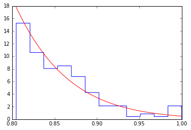
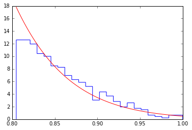
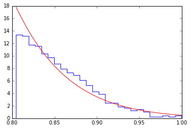
Figure 1: Histogram of the right edge of the spectrum of $A$ in the case of a homogenous Erdős-Rényi graph and density of (LABEL:dens). The eigenvalues are renormalized in such a way that $\lambda_{2}=1$ ($\lambda_{1}$ has been removed) and the histogram as well as the density are normalized in such a way that the total area is $1$. Here, $n=5\cdot 10^{4}$ and $d=0.5$ (left), $d=1.5$ (centre), $d=2.5$ (right). We see that as $d$ grows, the empirical density gets more convex at its edge, which agrees with the idea that the semicircle law approximation gets more accurate.

≲Fig:histo_edge

Remark 1.6.

The estimate (LABEL:EstN816) states there exists no deterministic sequence $\alpha=\alpha_{n}$ such that the point process

$$\Xi\mathrel{\vbox{\hbox{.}\hbox{.}}}=\{\alpha\lambda_{k}(\underline{A}\!\,)\mathrel{\vbox{\hbox{.}\hbox{.}}}k\in[n]\}$$

is asymptotically finite and nonzero on compact sets. In particular, $\Xi$ cannot converge to a point process as $n\to\infty$. Note, however, that our results do not rule out the existence of an affine transformation parametrized by $\alpha=\alpha_{n}$ and $\beta=\beta_{n}$ such that the point process $\{\alpha(\lambda_{k}(\underline{A}\!\,)-\beta)\mathrel{\vbox{\hbox{.}\hbox{.}}}k\in[n]\}$ converges.

1.3.  Consequences for the adjacency matrix

Gershgorin’s Circle Theorem implies that

$$\|\mathbb{E}A\|\leqslant d\,.$$

Then, writing $A=\underline{A}+\mathbb{E}A$, following corollary is an immediate consequence of Theorem LABEL:thalphall12 and Weyl’s inequality (see e.g. (Bhatia, , Corollary III.2.6)).

Corollary 1.7.

≲thalphall12cor

• Theorem LABEL:thalphall12 holds with $\underline{A}\!\,$ replaced by $A$ and the right-hand sides of (LABEL:Estlam816)–(LABEL:Estlam8160) replaced by $\displaystyle C\sqrt{np_{\max}}+\varepsilon\sqrt{L_{1}}+d$.

• Under (LABEL:eq:ordersA), w.h.p., for any $k\in[n]$,

  $${{\left|\lambda_{k}(A)-\lambda_{k}(\mathbb{E}A)\right|}}\leqslant C\Bigl{(}{\sqrt{L}_{1}+\sqrt{np_{\max}}}\Bigr{)}\,,$$

  for some universal constant $C$.

Remark 1.8.

As $L_{1}\sim D_{1}^{\downarrow}$, for an homogenous Erdős-Rényi random graph, Corollary LABEL:thalphall12cor is consistent with (MR1967486, , Theorem 1.1) which asserts that $\lambda_{1}(A)=\|A\|\sim\max\{\sqrt{D_{1}^{\downarrow}},d\}$ in all regimes of $d$.

1.4.  Applications to stochastic block models

In the stochastic block model, $\mathbb{E}A$ has bounded rank and all its nonzero eigenvalues are of order $d$. We denote by $\lambda_{1}^{+}\geqslant\cdots\geqslant\lambda_{k^{+}}^{+}>0$ the positive eigenvalues of $\mathbb{E}$ and $\lambda_{1}^{-}\leqslant\cdots\leqslant\lambda_{k^{-}}^{-}<0$ the negative eigenvalues of $\mathbb{E}A$. For $\kappa$ the constant of (LABEL:eq:ordersA), we suppose that

$$\la{541714h}d\geqslant\lambda_{1}^{+}\geqslant\cdots\geqslant\lambda_{k^{+}}^{+}\geqslant\kappa d\,,\quad-d\leqslant\lambda_{1}^{-}\leqslant\cdots\leqslant\lambda_{k^{-}}^{-}\leqslant-\kappa d\,,\quad k^{+}+k^{-}\leqslant\kappa^{-1}\,.$$ (1.11)

Then, there is a dichotomy in the behaviour of the $k^{+}+k^{-}$ largest (in absolute value) eigenvalues of $A$, depending on whether $d\ll\sqrt{L}_{1}$ or $d\gg\sqrt{L}_{1}$. Under mild conditions on $d$, these conditions read $d\ll\sqrt{\log n/\log\log n}$ or $d\gg\sqrt{\log n/\log\log n}$.

Proposition 1.9.

≲propo:SBMLet $\varepsilon\in(0,1)$.

1. Under conditions (LABEL:eq:ordersA) and $d\leqslant\eta\sqrt{\log n/\log\log n}$, w.h.p.

   $$\la{propo:SBM1}\|A\|\leqslant(1+\varepsilon)\sqrt{L}_{1}+C\sqrt{np_{\max}}\,.$$ (1.12)

   Under the additional conditions $d_{i}=d$ for all $i$ and $np_{\max}\leqslant\eta L_{1}$, we have for all $k\in[n^{1-\varepsilon}]$

   $$\la{propo:SBM2}\lambda_{k}(A)\sim\sqrt{L_{k}}\and\lambda_{n+1-k}(A)\sim-\sqrt{L_{k}}\,.$$ (1.13)

2. Under conditions (LABEL:eq:ordersA), (LABEL:541714h), and $d\geqslant\eta^{-1}\sqrt{\log n/\log\log n}$,

   $$\la{propo:SBM3}\forall i=1,\ldots,k^{+}\,,\quad\lambda_{i}(A)\sim\lambda^{+}_{i}\,,\qquad\qquad\forall i=1\,,\ldots,k^{-}\,,\quad\lambda_{n+1-i}(A)\sim\lambda^{-}_{i}$$ (1.14)

   and w.h.p.,

   $$\la{propo:SBM4}\max\{|\lambda_{k^{+}+1}(A)|,|\lambda_{n-k^{-}}(A)|\}\leqslant(1+\varepsilon)\sqrt{L}_{1}+C\sqrt{np_{\max}}\,.$$ (1.15)

   Under the additional conditions $d_{i}=d$ for all $i$ and $np_{\max}\leqslant\eta L_{1}$, we have for all $k\in[n^{1-\varepsilon}]$

   $$\la{propo:SBM5}\lambda_{k^{+}+k}(A)\sim\sqrt{L_{k}}\and\lambda_{n+1-(k^{-}+k)}(A)\sim-\sqrt{L_{k}}\,.$$ (1.16)

We remark that in the case (a) of small degree, the nontrivial eigenvalues $\lambda^{\pm}_{i}$ of $\mathbb{E}A$ do not give rise to corresponding eigenvalues of $A$, and $A$ may be regarded as a perturbation of $\underline{A}\!\,$. In contrast, in the case (b) of large degree, the nontrivial eigenvalues $\lambda^{\pm}_{i}$ of $\mathbb{E}A$ gives rise to associated outlier eigenvalues of $A$, and $A$ may be regarded as a perturbation of $\mathbb{E}A$. Hence, the spectrum of $A$ retains some information about the spectrum of $\mathbb{E}A$ if and only if $d\gg\sqrt{\log n/\log\log n}$.

Remark 1.10.

Remarks LABEL:rem:pospart2 and 1.6 also hold for the eigenvalue counting measure of $A$. See Figure LABEL:Fig:histo_edge for an illustration.

Proof of Proposition LABEL:propo:SBM.

The proof is a simple consequence of the results of the preceding subsections and of Weyl’s inequalities. More specifically, use (Bhatia, , Corollary III.2.6) to prove (LABEL:propo:SBM1), (LABEL:propo:SBM2), (LABEL:propo:SBM3) and (LABEL:propo:SBM4) considering $A$ as a perturbation of $\underline{A}$ in (a) and $A$ as a perturbation of $\mathbb{E}A$ in (b). To prove the first part of (LABEL:propo:SBM5) (the second part can be proved in the same way), note that by (Bhatia, , Corollary III.2.3 and Exercise III.2.4) we have, for any $k$,

$$\lambda_{k+2k^{+}+k^{-}}(\underline{A})\leqslant\lambda_{k^{+}+k}(A)\leqslant\lambda_{k}(\underline{A})$$

and use Corollary 1.4. ∎

1.5.  Behaviour of the largest degrees

In our regime of interest, the largest degrees of the graph play a key role in the analysis of the largest eigenvalues of the adjacency matrix. We now describe their asymptotic behavior.

Proposition 1.11.

≲propo_position_degree_max Let $\varepsilon\in(0,1)$. Under (LABEL:eq:ordersA), w.h.p., for any $k\in[n^{1-\varepsilon}]$

$$D_{k}^{\downarrow}\leqslant(1+\varepsilon)L_{k}\,.$$

For any $x>0$, we introduce the sets

$$\la{def:usoleq0V}\mathcal{V}_{\geqslant x}\mathrel{\vbox{\hbox{.}\hbox{.}}}=\{i\in[n]\,:\,D_{i}\geqslant x\}\,,\qquad\mathcal{V}_{=x}\mathrel{\vbox{\hbox{.}\hbox{.}}}=\{i\in[n]\,:\,D_{i}=x\}\,.$$ (1.17)

These sets are related to the ordered degrees through

$$\la{641710h}D^{\downarrow}_{k}\geqslant x\iff\#\mathcal{V}_{\geqslant x}\geqslant k\,.$$ (1.18)

Let us introduce the function $f$ on $(d,\infty)$ defined by

$$f(x)=f_{d}(x)\mathrel{\vbox{\hbox{.}\hbox{.}}}=x\log{{\left(\frac{x}{d}\right)}}-(x-d)-\log\sqrt{2\pi x}\,.$$ (1.19)

If $Y$ is a Poisson random variable with mean $d$, for a large integer $x$ Stirling’s approximation gives

$$\mathbb{P}(Y=x)=\mathrm{e}^{-f(x)+O(x^{-1})}\,.$$ (1.20)

We shall in fact prove that, roughly speaking, under condition (LABEL:eq:ordersA), we have

$$\la{641710h10}\#\mathcal{V}_{\geqslant x}\lesssim n\mathrm{e}^{f(x)}\,,$$ (1.21)

which, under the additional assumption $d_{i}=d$ for all $i$, can be strengthened to

$$\la{641710h11}\#\mathcal{V}_{\geqslant x}\approx n\mathrm{e}^{f(x)}\,.$$ (1.22)

This leads us to introduce, for $k\in[n]$, the solution $\Delta_{k}$ of the equation

$$f(\Delta_{k})=\log(n/k)\and\Delta_{k}\geqslant d\,.$$

This solution is unique and satisfies

$$\Delta_{k}\sim L_{k}\,.$$ (1.23)

(See Lemma LABEL:LCDBMLEV below for the full details.) The combination of the characterization (LABEL:641710h) of the largest degrees with estimates (LABEL:641710h10), (LABEL:641710h11) and (1.23) naturally leads to the estimates given in Propositions LABEL:propo_position_degree_max and LABEL:27516.

In the special case of a homogenous Erdős-Rényi graph, the next proposition is essentially contained in (MR1864966, , Chapter 3). Hence, our next result may be viewed as a generalization of this result to the inhomogeneous case. It is a more precise version of Proposition LABEL:propo_position_degree_max under the additional assumption that all vertices have the same mean degree.

Proposition 1.12.

≲27516 Let $\varepsilon\in(0,1)$.

• For any $k\in[n^{1-\varepsilon}]$ there exists a deterministic $\Delta^{\prime}_{k}\in\{\lfloor\Delta_{k}\rfloor,\lceil\Delta_{k}\rceil\}$ such that under the conditions $d_{i}=d$ for all $i$ and (LABEL:eq:ordersA), w.h.p., for any $k\in[n^{1-\varepsilon}]$, we have

  1. $D^{\downarrow}_{k}\in\{\Delta^{\prime}_{k},\Delta^{\prime}_{k}-1\}$,

  2. $D^{\downarrow}_{k}=\lfloor\Delta_{k}\rfloor$ when $\mathrm{dist}(\Delta_{k},\mathbb{N})\geqslant\varepsilon$.

• Under the conditions $d_{i}=d$ for all $i$ and (LABEL:eq:ordersA), for all integers $t\in[\varepsilon\Delta_{1},\Delta_{1}-\varepsilon]$,

  $$\la{estimate:cardVka}\#\mathcal{V}_{\geqslant t}\sim\#\mathcal{V}_{=t}\sim n\mathrm{e}^{-f(t)}\,.$$ (1.24)

  Under the same conditions, if $t\geqslant\Delta_{1}+\varepsilon$ then, w.h.p., $\#\mathcal{V}_{\geqslant t}=0$.

An immediate corollary of Proposition LABEL:27516 and (1.23) is the following.

Corollary 1.13.

Let $\varepsilon\in(0,1)$. Under the conditions $d_{i}=d$ for all $i$ and (LABEL:eq:ordersA), for all $k\in[n^{1-\varepsilon}]$,

$$D_{k}^{\downarrow}\sim L_{k}\,.$$

Remark 1.14 (Lack of limit point process of largest degrees).

≲noPoisson Proposition LABEL:27516 (b) shows that, perhaps surprisingly, there is no Poisson point process at the right edge of the multiset of degrees of $G$. There is instead a sharp transition at $\Delta_{1}$: for any integer $t\leqslant\Delta_{1}-\varepsilon$, w.h.p. the number of vertices with degree $t$ is $\gg 1$ and for any integer $t\geqslant\Delta_{1}+\varepsilon$, w.h.p. there is no vertex with degree $t$.

2 Estimation of the largest degrees and comparison with the eigenvalues

The rest of this paper is devoted to the proofs of our main results.

Throughout this section we use the following conventions about convergence of deterministic quantities. Let $u$ and $v$ be deterministic quantities depending on $n$ and $(p_{ij})_{i,j\in[n]}$. We write $u=o(v)$, or, equivalently, $u\ll v$, whenever $u/v\to 0$ as $n\to\infty$ and $\eta\to 0$, uniformly in $(p_{ij})_{i,j\in[n]}$ satisfying (LABEL:eq:ordersA) and all parameters except $\varepsilon$. We remark that such a convergence can always be upgraded to a quantitative convergence using some admissible error function from Definition LABEL:def:error_control, but for the sake of simplicity we shall not do this.

2.1.  Largest degrees: proof of Proposition LABEL:propo_position_degree_max and Proposition LABEL:27516

Recall that the function $f$ was defined in (1.19).

Lemma 2.1.

≲LCDBMLEV Let $\varepsilon\in(0,1)$. For $n$ large enough and $\eta$ small enough, under condition (LABEL:eq:ordersA), for any $k\in[n^{1-\varepsilon}]$, there exists a unique solution $\Delta_{k}$ of the equation

$$\la{def:usoleq0}f(\Delta_{k})=\log(n/k)\and\Delta_{k}\geqslant d\,.$$ (2.1)

Moreover, under condition (LABEL:eq:ordersA), for any $k\in[n^{1-\varepsilon}]$,

$$\Delta_{k}\sim L_{k}\,.$$ (2.2)

Proof.

The function $f$ is increasing on $(d,\infty)$ (indeed, $f^{\prime}(u)=\log(u/d)+1/(2u)$) and satisfies

$$\la{f:est1}f(u)=u\log(u/d)+O(u)\qquad\textrm{ as $u\to\infty$}\,,$$ (2.3)

so that for $n$ large enough, $\Delta_{k}$ is well defined for any $1\leqslant k\leqslant n^{1-\varepsilon}$. Moreover, (unconditionally on $d$), we have

$$\la{f:est2}f(u+x)=f(u)+x\log(u/d)+O(x/u+x^{2}/u)\,.$$ (2.4)

Indeed,

$$f(u+x)-f(u)=(u+x)\log\left(1+\frac{x}{u}\right)+x\log{{\left(\frac{u}{d}\right)}}-x+\frac{1}{2}\log\Bigl{(}{1+\frac{x}{u}}\Bigr{)}\,.$$ (2.5)

Let us now prove (2.2). As both $\Delta_{k}=\Delta_{k}(n,d)$ and $L_{k}=L_{k}(n,d)$ are deterministic and depend only on $n$ and $d$, by Definition LABEL:def:error_control, (2.2) reads

$$\la{04041712h}\lim_{\begin{subarray}{c}n\to\infty\\ \eta\to 0\end{subarray}}\sup_{\kappa\leqslant d\leqslant\eta\log n}\sup_{k\in[n^{1-\varepsilon}]}\left|\frac{\Delta_{k}(n,d)}{L_{k}(n,d)}-1\right|=0\,.$$ (2.6)

If it were not the case, there would be an infinite set $I$ of positive integers and some sequences $(\eta_{n})_{n\in I},(d_{n})_{n\in I},(k_{n})_{n\in I}$ satisfying $\kappa\leqslant d_{n}\leqslant\eta_{n}\log n$, $1\leqslant k_{n}\leqslant n^{1-\varepsilon}$ and $\eta_{n}\to 0$ as $n\in I$ tends to infinity, such that

$$\la{441714h22}\left|\frac{\Delta_{k_{n}}(n,d_{n})}{L_{k}(n,d_{n})}-1\right|>c$$ (2.7)

for some positive constant $c$. Let us drop the index $n$ from the notation. One first verifies that $\Delta_{k}/d\to\infty$ as $n\in I$ grows (by a simple argument by contradiction using (LABEL:def:usoleq0)). Then, introduce $\varphi>0$ such that $\Delta_{k}=\varphi L_{k}.$ By (LABEL:f:est1), we have

$$\log(n/k) =f\left(\Delta_{k}\right)$$

$$\sim\Delta_{k}\log(\Delta_{k}/d)$$

$$=\varphi\frac{\log(n/k)}{\log((\log n)/d)}\bigl{(}{\log(\log(n/k)/d)+\log\varphi-\log\log((\log n)/d)}\bigr{)}\,.$$

By assumption, $\varepsilon\log n\leqslant\log(n/k)\leqslant\log n$ so that

$$\la{1291112}\frac{1}{\varphi}\sim 1+\frac{\log\varphi}{\log((\log n)/d)}+o(1)\,.$$ (2.8)

On easily deduces from (LABEL:1291112) that $\varphi$ is bounded away from $0$ and $\infty$, and then that $\varphi$ tends to one, which contradicts (LABEL:441714h22). Thus (LABEL:04041712h), hence also (2.2), are true. ∎

Lemma 2.2.

≲LCDBMLEVBIS Suppose that $n$ is large enough and $\eta$ small enough, and that $d$ satisfies condition (LABEL:eq:ordersA), so that $\Delta_{1}$ is well defined (see Lemma LABEL:LCDBMLEV). Let $q_{1},\dots,q_{n}>0$ satisfy $d=\sum_{i}q_{i}$, and let $X$ be a random variable with law $\mathrm{Bin}(q_{1},\ldots,q_{n})$. Suppose that $q_{\max}\mathrel{\vbox{\hbox{.}\hbox{.}}}=\max_{i}q_{i}\leqslant d/(\log n)^{5/2}$. Then for any $u\leqslant\Delta_{1}$ and $x$ such that $x^{2}\leqslant u$ and $u+x\geqslant 2d$ is integer,

$$\la{AsexpTail}\mathbb{P}(X\geqslant u+x)={{\left(1+\delta\right)}}{{\left(\frac{u}{d}\right)}}^{-x}\mathrm{e}^{-f(u)}\,.$$ (2.9)

where $\delta=O{{\left((d+x^{2})/u+q_{\max}u^{5/2}/d\right)}}$.

Proof.

By Theorem 3.1 below, $\mathbb{P}(X\geqslant u+x)={{\left(1+\delta\right)}}\mathbb{P}(Y=u+x)$ where $Y$ has Poisson distribution with mean $d$ and $\delta=O{{\left(d/u+q_{\max}u^{5/2}/d\right)}}$. Now, by (1.20), we have

$$\mathbb{P}(Y=u+x)=\mathrm{e}^{-f(u+x)+O(1/u)}\,.$$ (2.10)

Then, the estimate (LABEL:f:est2) allows to conclude.∎

We are now ready to prove Proposition LABEL:propo_position_degree_max.

Proof of Proposition LABEL:propo_position_degree_max.

Let $k\in[n^{1-\varepsilon}]$. It is sufficient to prove that w.h.p. we have $D_{k}^{\downarrow}\leqslant(1+\varepsilon)L_{k}$. Indeed, the inversion of w.h.p. and for all $k\in[n^{1-\varepsilon}]$ is straightforward using $k=n^{1-\ell\varepsilon}$ for each $\ell\in[1/\varepsilon]$, as all error terms $o(1)$ in what follows are terms tending to zero uniformly in $k\in[n^{1-\varepsilon}]$ as $n\to\infty$ and $\eta\to 0$.

We note that $D^{\downarrow}_{k}\geqslant t$ is equivalent to $\#\mathcal{V}_{\geqslant t}\geqslant k$ (the set $\mathcal{V}_{\geqslant t}$ has been defined in (LABEL:def:usoleq0V)). By (LABEL:f:est2), we have

$$n\mathrm{e}^{-f(\Delta_{k}+x)}=k(1+o(1))(\Delta_{k}/d)^{-x}\,.$$ (2.11)

Thus (2.11) applied to $x=\lfloor\Delta_{k}\rfloor+2-\Delta_{k}$ implies that $n\mathrm{e}^{-f(\lfloor\Delta_{k}\rfloor+2)}=o(k)$. By (LABEL:AsexpTail) in Lemma LABEL:LCDBMLEVBIS, it follows that $\mathbb{E}\#\mathcal{V}_{\geqslant t}=o(k)$ if $t=\lfloor\Delta_{k}\rfloor+2$. It remains to use (2.2) and Markov’s inequality. ∎

Our proof of Proposition LABEL:27516 will require a sharp bound on the variance of $\#\mathcal{V}_{\geqslant t}$.

Lemma 2.3.

≲estimate_variance Let $D_{i}$ denote the degree of the vertex $i$ in the graph $G$. Then any integer $t\geqslant 0$,

$$\operatorname{Var}(\#\mathcal{V}_{\geqslant t})\leqslant\mathbb{E}\#\mathcal{V}_{\geqslant t}+3dn\max_{i}\mathbb{P}(D_{i}\geqslant t-1)^{2}\,.$$

Proof.

For ease of notation, we set $q_{i}:=\mathbb{P}(D_{i}\geqslant t)$. Since $\#\mathcal{V}_{\geqslant t}=\sum_{i=1}^{n}\mathbbm{1}_{D_{i}\geqslant t}$, we have $\mathbb{E}\#\mathcal{V}_{\geqslant t}=\sum_{i=1}^{n}q_{i}$ and

$$\operatorname{Var}(\#\mathcal{V}_{\geqslant t}) =\sum_{i,j}\operatorname{Cov}(\mathbbm{1}_{D_{i}\geqslant t},\mathbbm{1}_{D_{j}\geqslant t})$$

$$=\sum_{i}q_{i}(1-q_{i})+\sum_{i\neq j}\operatorname{Cov}(\mathbbm{1}_{D_{i}\geqslant t},\mathbbm{1}_{D_{j}\geqslant t})\,.$$

Hence it suffices to prove that for $i\neq j$,

$$\la{66161}\operatorname{Cov}(\mathbbm{1}_{D_{i}\geqslant t},\mathbbm{1}_{D_{j}\geqslant t})\leqslant 3p_{ij}\max_{i}\mathbb{P}(D_{i}\geqslant t-1)^{2}\,.$$

Let us fix $i\neq j$. We have $D_{i}=\sum_{k}A_{ik}$ and $D_{j}=\sum_{k}A_{jk}$. We introduce the events

$$E\mathrel{\vbox{\hbox{.}\hbox{.}}}=\left\{\sum_{k\neq j}A_{ik}\geqslant t,A_{ij}=0\right\}\,,\qquad E^{\prime}\mathrel{\vbox{\hbox{.}\hbox{.}}}=\left\{\sum_{k}A_{ik}\geqslant t\right\}\,,$$

$$F\mathrel{\vbox{\hbox{.}\hbox{.}}}=\left\{\sum_{k\neq i}A_{jk}\geqslant t,A_{ij}=0\right\}\,,\qquad F^{\prime}\mathrel{\vbox{\hbox{.}\hbox{.}}}=\left\{\sum_{k}A_{jk}\geqslant t\right\}\,.$$

Then $E\subset E^{\prime}$, $F\subset F^{\prime}$ and $(E^{\prime}\backslash E)\cap F=(F^{\prime}\backslash F)\cap E=\emptyset$, the latter follows from $E^{\prime}\backslash E=\{\sum_{k\neq j}A_{ik}\geqslant t-1,A_{ij}=1\}$ (and similarly for $F^{\prime}\backslash F$). Thus by Lemma LABEL:lem:covBernoulli and the independence of the events $\{\sum_{k\neq j}A_{ik}\geqslant s\}$ and $\{\sum_{k\neq i}A_{jk}\geqslant s^{\prime}\}$

$$\operatorname{Cov}(\mathbbm{1}_{D_{i}\geqslant t},\mathbbm{1}_{D_{j}\geqslant t}) =\operatorname{Cov}(\mathbbm{1}_{E^{\prime}},\mathbbm{1}_{F^{\prime}})$$

$$\leqslant\mathbb{P}\bigl{(}{(E^{\prime}\backslash E)\cap(F^{\prime}\backslash F)}\bigr{)}+\mathbb{P}(F^{\prime}\backslash F)\mathbb{P}(E)+\mathbb{P}(E^{\prime}\backslash E)\mathbb{P}(F)$$

$$\leqslant 3p_{ij}\mathbb{P}\biggl{(}{\sum_{k\neq j}A_{ik}\geqslant t-1}\biggr{)}\mathbb{P}\biggl{(}{\sum_{k\neq i}A_{jk}\geqslant t-1}\biggr{)}\,,$$

which allows to conclude. ∎

We are ready to prove Proposition LABEL:27516.

Proof of Proposition LABEL:27516.

First we remark that the inversion of w.h.p. and for all for all integers $t\in[\varepsilon\Delta_{1},\Delta_{1}-\varepsilon]$ for (b) or for all $k\in[n^{1-\varepsilon}]$ for (a) can be treated as in the proof of Proposition LABEL:propo_position_degree_max.

• By (LABEL:AsexpTail) in Lemma LABEL:LCDBMLEVBIS, if $t\geqslant\Delta_{1}+\varepsilon$, $\mathbb{P}(\#\mathcal{V}_{\geqslant t}\geqslant 1)\leqslant\mathbb{E}\#\mathcal{V}_{\geqslant t}\leqslant(1+\varepsilon)(d/\Delta_{1})^{\varepsilon}$ tends to $0$. Moreover, in the regime $\varepsilon\Delta_{1}\leqslant t\leqslant\Delta_{1}-\varepsilon$, as $n\mathrm{e}^{-f(t)}$ goes to infinity, to prove the left-hand side of (LABEL:estimate:cardVka), by Markov’s inequality it suffices to prove that $\mathbb{E}\#\mathcal{V}_{\geqslant t}=n\mathrm{e}^{-f(t)}(1+o(1))$ and $\operatorname{Var}(\#\mathcal{V}_{\geqslant t})=n\mathrm{e}^{-f(t)}(1+o(1))$, which follows directly from (LABEL:AsexpTail) in Lemma LABEL:LCDBMLEV and Lemma LABEL:estimate_variance.

  It remains to prove that $\#\mathcal{V}_{=t}\sim n\mathrm{e}^{-f(t)}$ when $\varepsilon\Delta_{1}\leqslant t\leqslant\Delta_{1}-\varepsilon$. We note that

  $$\#\mathcal{V}_{=t}=\#\mathcal{V}_{\geqslant t}-\#\mathcal{V}_{\geqslant t+1}\,.$$

  From what precedes, it suffices to check that $\#\mathcal{V}_{t+1}=o(n\mathrm{e}^{-f(t)})$. The latter is a consequence of (LABEL:AsexpTail) in Lemma LABEL:LCDBMLEV which implies that $\mathbb{E}\#\mathcal{V}_{t+1}\leqslant(1+o(1))(d/t)n\mathrm{e}^{-f(t)}$.

• We note that for any $k,t$, the claim $D^{\downarrow}_{k}\geqslant t$ is equivalent to $\#\mathcal{V}_{\geqslant t}\geqslant k$. Thus (2.11) applied to $x=\lfloor\Delta_{k}\rfloor-1-\Delta_{k}$ and (b) imply that with high probability $D^{\downarrow}_{k}\geqslant\lfloor\Delta_{k}\rfloor-1$. Similarly, (2.11) applied to $x=\lfloor\Delta_{k}\rfloor+2-\Delta_{k}$ and (b) imply with high probability $D^{\downarrow}_{k}\leqslant\lfloor\Delta_{k}\rfloor+1$. Moreover, if $\lfloor\Delta_{k}\rfloor+1-\Delta_{k}\geqslant\varepsilon$, then with high probability $D^{\downarrow}_{k}\leqslant\lfloor\Delta_{k}\rfloor$, while if $\lfloor\Delta_{k}\rfloor-\Delta_{k}\leqslant-\varepsilon$ then with high probability $D^{\downarrow}_{k}\geqslant\lfloor\Delta_{k}\rfloor$. Note that either $\lfloor\Delta_{k}\rfloor-\Delta_{k}\leqslant-\varepsilon$ or $\lfloor\Delta_{k}\rfloor+1-\Delta_{k}\geqslant\varepsilon$ holds when $\varepsilon=1/2$. ∎

2.2.  Proof of Theorem LABEL:thalphall12

First it is easy to see, by Weyl’s inequality, that we may assume without loss of generality that $p_{ii}=0$ for all $i\in[n]$. As pointed in introduction, our strategy is to describe the graph spanned by the vertices of high degree. We start with a deviation inequality on the degrees. Define

$$h(x)\;\mathrel{\vbox{\hbox{.}\hbox{.}}}=\;(1+x)\log(1+x)-x\,.$$ (2.12)

Lemma 2.4.

For distinct $i_{1},\ldots,i_{k}\in[n]$ and $t\geqslant 0$ we have

$$\mathbb{P}\left(\sum_{\ell=1}^{k}D_{i_{\ell}}\geqslant k(d+t)\right)\leqslant\exp\left(-kdh\left(\frac{t}{d}\right)+k^{2}p_{\max}\left(\frac{t}{d}+1\right)^{2}\right)\,.$$ (2.13)

In particular, if $d\ll t$ and $kt/\log(t/d)\ll d^{2}/p_{\max}$, we have

$$\mathbb{P}\left(\sum_{\ell=1}^{k}D_{i_{\ell}}\geqslant kt\right)\leqslant\exp\left(-(1+o(1))kt\log\left(\frac{t}{d}\right)\right)\,.$$ (2.14)

Proof.

We have

$$\mathbb{P}\left(\sum_{\ell=1}^{k}D_{i_{\ell}}\geqslant k(d+t)\right)\leqslant\mathbb{P}\left(\sum_{\ell=1}^{k}D_{i_{\ell}}-\mathbb{E}D_{i_{\ell}}\geqslant kt\right)\,.$$

Now,

$$\sum_{\ell=1}^{k}D_{i_{\ell}}=2\sum_{\ell=1}^{k}\sum_{j=\ell+1}^{k}A_{i_{\ell}i_{j}}+\sum_{\ell=1}^{k}\sum_{j\notin\{i_{1},\ldots,i_{k}\}}A_{i_{\ell}j}=\mathrel{\vbox{\hbox{.}\hbox{.}}}2S_{1}+S_{2}\,,$$

where $S_{1}$ and $S_{2}$ are independent. From Chernov’s bound, for any $\lambda\geqslant 0$,

$$\mathbb{P}\left(\sum_{\ell=1}^{k}D_{i_{\ell}}-\mathbb{E}D_{i_{\ell}}\geqslant kt\right)\leqslant\exp(-\lambda kt+\alpha\phi(\lambda)+\beta\phi(2\lambda)),$$

where $\phi(\lambda)=\mathrm{e}^{\lambda}-\lambda-1$,

$$\alpha=\sum_{\ell=1}^{k}\sum_{j\notin\{i_{1},\ldots,i_{k}\}}p_{i_{\ell}j}\and\beta=2\sum_{\ell=1}^{k}\sum_{j=\ell+1}^{k}p_{i_{\ell}i_{j}}=\sum_{\ell=1}^{k}\sum_{j=1}^{k}p_{i_{\ell}i_{j}}\,.$$

By hypothesis, $\alpha+\beta\leqslant kd$ and $\beta\leqslant k^{2}p_{\max}$. We take $\lambda=\log(t/d+1)$ and use that $\phi(2\lambda)\leqslant e^{2\lambda}$, we arrive at (2.13). The second claim (2.14) is an immediate consequence of the fact that the function $h$ from (2.12) satisfies $h(x)\sim x\log x$ when $x$ goes to infinity. ∎

Lemma 2.5.

There exists a constant $c>0$ such that the following holds. Let $\varepsilon\in(0,1)$ and $t=\varepsilon L_{1}$. For $S\subset\{1,\ldots,n\}$, let $\mathcal{N}(S)=\{j:A_{ij}=1\hbox{ for some }i\in S\}$ denote the set of neighbours of elements in $S$. Then, under (LABEL:eq:ordersA), w.h.p. for any $i\in\mathcal{V}_{\geqslant t}$ we have

$$\#\bigl{[}{\mathcal{N}(i)\cap\left(\mathcal{V}_{\geqslant t}\cup\mathcal{N}(\mathcal{V}_{\geqslant t}\backslash\{i\})\right)}\bigr{]}\leqslant c/\varepsilon\,.$$

Proof.

Fix an integer $k$. Let $P(1)$ be the probability that there exists a vertex of $\mathcal{V}_{\geqslant t}$ which is neighbour to at least $k$ other elements of $\mathcal{V}_{\geqslant t}$. We have

$$P(1) \leqslant\sum_{\begin{subarray}{c}i_{0},\ldots,i_{k}\\ \textrm{distinct}\end{subarray}}\mathbb{P}{{\left(D_{i_{0}}\geqslant t\;\hbox{ and }\;\forall\ell\in\{0,\ldots,k\}:D_{i_{\ell}}\geqslant t,A_{i_{0}i_{\ell}}=1\right)}}$$

$$\leqslant\ \sum_{\begin{subarray}{c}i_{0},\ldots,i_{k}\\ \textrm{distinct}\end{subarray}}\mathbb{P}{{\left(D_{i_{0}}\geqslant t-k\right)}}\mathbb{P}{{\left(\forall\ell\in\{1,\ldots,k\}:D_{i_{\ell}}\geqslant t-1\right)}}\prod_{\ell=1}^{k}p_{i_{0}i_{\ell}}$$

Since for any fixed $i_{0}$ we have

$$\la{23101612h}\sum_{\begin{subarray}{c}i_{1},\ldots,i_{k}\\ \textrm{distinct}\end{subarray}}\prod_{\ell=1}^{k}p_{i_{0}i_{\ell}}\leqslant d^{k}$$ (2.15)

we deduce that

$$P(1) \leqslant nd^{k}\max_{i}\mathbb{P}{{\left(D_{i}\geqslant t-k\right)}}\max_{\begin{subarray}{c}i_{1},\ldots,i_{k}\\ \textrm{distinct}\end{subarray}}\mathbb{P}{{\left(\forall\ell\in\{1,\ldots,k\}:D_{i_{\ell}}\geqslant t-1\right)}}$$

$$\leqslant nd^{k}\exp\left(-(1+o(1))(k+1)t\log\frac{t}{d}\right)$$

if $t\gg d$ and $tp_{\max}\ll d^{2}\log(t/d)$ (from (2.14)). For $t=\varepsilon L_{1}\gg d$ and $k$ fixed such that $k+1>a/\varepsilon$ with $a>1$. We find

$$P(1)\leqslant n^{1-a(1+o(1))}=o(1)\,.$$

Similarly, let $P(2)$ be the probability that there exists a vertex $i\in\mathcal{V}_{\geqslant t}$ which is neighbour to at least $k$ elements of $\mathcal{N}(\mathcal{V}_{\geqslant t}\backslash\{i\})$. Then

$$P(2)\leqslant \sum_{s=1}^{k}\sum_{\tau}\sum_{\begin{subarray}{c}i_{0},\ldots,i_{s},j_{1},\ldots,j_{k}\\ \textrm{distinct}\end{subarray}}\mathbb{P}{{\left(D_{i_{0}},\ldots,D_{i_{s}}\geqslant t\hbox{ and }\;\forall\ell=1,\ldots,k:A_{i_{0}j_{\ell}}=A_{j_{\ell}i_{\tau(\ell)}}=1\right)}}\,,$$

where the second sum is over all surjective maps $\tau:\{1,\ldots,k\}\to\{1,\ldots,s\}$. We deduce that

$$P(2) \leqslant\sum_{s=1}^{k}\sum_{\tau}\sum_{\begin{subarray}{c}i_{0},\ldots,i_{s},j_{1},\ldots,j_{k}\\ \textrm{distinct}\end{subarray}}\mathbb{P}{{\left(D_{i_{0}}\geqslant t-s\right)}}\mathbb{P}{{\left(\forall r\in\{1,\ldots,s\}:D_{i_{r}}\geqslant t-\#\tau^{-1}(\{r\})\right)}}\prod_{\ell=1}^{k}p_{i_{0}j_{\ell}}p_{j_{\ell}i_{\tau(\ell)}}\,.$$

Now, note that for any fixed surjective map $\tau:[k]\to[s]$,

• for any $i_{1},\ldots,i_{s}$, we have

  $$\left\{\forall r\in\{1,\ldots,s\}:D_{i_{r}}\geqslant t-\#\tau^{-1}(\{r\})\right\}\subset\left\{\sum_{r=1}^{s}D_{i_{r}}\geqslant st-k\right\}\,;$$

• for any fixed $j_{1},\ldots,j_{k}$, we have, as in (LABEL:23101612h),

  $$\sum_{\begin{subarray}{c}i_{1},\ldots,i_{s}\\ \textrm{distinct}\end{subarray}}\prod_{\ell=1}^{k}p_{j_{\ell}i_{\tau(\ell)}}\leqslant d^{s}p_{\max}^{k-s}\,.$$

We deduce, using (LABEL:23101612h) and (2.14) again, that

$$P(2) \leqslant\sum_{s=1}^{k}\sum_{\tau}nd^{k+s}p_{\max}^{k-s}\max_{i}\mathbb{P}{{\left(D_{i}\geqslant t-k\right)}}\max_{\begin{subarray}{c}i_{1},\ldots,i_{s}\\ \textrm{distinct}\end{subarray}}\mathbb{P}{{\left(\sum_{\ell=1}^{s}D_{i_{\ell}}\geqslant st-k\right)}}$$

$$\leqslant nd^{k}\sum_{s=1}^{k}{k\choose s}k^{k-s}d^{s}p_{\max}^{k-s}\mathrm{e}^{-(1+o(1))(s+1)t\log\left(\frac{t}{d}\right)}\,.$$

The $o(1)$ is uniform over $1\leqslant s\leqslant k$. Hence,

$$P(2)\leqslant nd^{k}\mathrm{e}^{-(1+o(1))t\log\left(\frac{t}{d}\right)}\left(d\mathrm{e}^{-(1+o(1))t\log\left(\frac{t}{d}\right)}+kp_{\max}\right)^{k}\,.$$

As above for $t=\varepsilon L_{1}\gg d$ and $k$ a fixed integer such that $k+1>a/\varepsilon$ with $a>1$. We find $P(2)=o(1).$ This concludes the proof of the first claim of the lemma. ∎

Definition 2.6.

A star graph with central degree $D$ is the graph with vertex set $\{0,1,\dots,D\}$ and edge set $\{\{0,1\},\{0,2\},\dots,\{0,D\}\}$.

We may now prove Theorem LABEL:thalphall12.

Proof of Theorem LABEL:thalphall12.

Let $0<\delta<\varepsilon$ and set $t:=\delta L_{1}$. By Proposition LABEL:propo_position_degree_max, w.h.p. for any $k\in[n^{1-\varepsilon}]$,

$$D^{\downarrow}_{k}\geqslant t\,.$$

Let $G_{\star}$ be the graph obtained from $G$ as follows. The vertex set of $G_{\star}$ is $[n]$. The edge set of $G_{\star}$ is the set of edges $\{i,j\}$ of $G$ (i.e. $A_{ij}=1$) such that $i\in\mathcal{V}_{\geqslant t}$ and $j\notin\mathcal{V}_{\geqslant t}\cup\mathcal{N}(\mathcal{V}_{\geqslant t}\backslash\{i\})$ (where the notation $\mathcal{N}(\cdot)$ was introduced in Lemma 2.5). By construction, $G_{\star}$ is a disjoint union of isolated vertices and of star graphs with central degrees $D_{i}^{\star}$, $i\in\mathcal{V}_{\geqslant t}$. By Lemma 2.5, w.h.p., the central degrees of the stars satisfy $D_{i}-c/\delta\leqslant D_{i}^{\star}\leqslant D_{i}$. Let $A_{\star}$ be the adjacency matrix of $G_{\star}$ and let $A^{\prime}=A-A_{\star}$ be the adjacency matrix of $G\backslash G_{\star}$.

By Lemma LABEL:StarGraph, the nonzero eigenvalues of $A_{\star}$ are $\pm\sqrt{D^{\star}_{i}}$, $i\in\mathcal{V}_{\geqslant t}$. From what precedes, w.h.p. for all $i\in\mathcal{V}_{\geqslant t}$,

$$\la{eq231019h30}\left|\sqrt{D^{\star}_{i}}-\sqrt{D_{i}}\right|=\frac{D_{i}-D_{i}^{\star}}{\sqrt{D_{i}}+\sqrt{D_{i}^{\star}}}\leqslant\frac{c}{\delta\sqrt{t}}\,.$$ (2.16)

for $c$ the universal constant of Lemma 2.5.

Besides, w.h.p. the maximal degree in $G\backslash G_{\star}$ is bounded by $\max(t,c/\delta)$. Indeed, let $i\in[n]$ be a vertex. If the degree of $i$ in $G$ is $<t$, then there is nothing to prove (as the degree of $i$ in $G\backslash G_{\star}$ is bounded by its degree in $G$), whereas if $D_{i}\geqslant t$, then the degree of $i$ in $G\backslash G_{\star}$ is $D_{i}-D_{i}^{\star}\leqslant c/\delta$.

By Proposition LABEL:27516, we know that w.h.p., the cardinal number of $\mathcal{V}_{\geqslant t}$ is at most $n^{1-\delta+o(1)}\leqslant 10/p_{\max}$, hence by Theorem LABEL:LeVer of Le, Levina, and Vershynin, w.h.p.

$$\la{eq8juin19h30}\|A^{\prime}-\mathbb{E}A\|\leqslant C((np_{\max})^{1/2}+(\delta L_{1})^{1/2})\,.$$ (2.17)

Then, one concludes thanks to Weyl’s perturbation inequality (see e.g. (Bhatia, , Corollary III.2.6)), noticing that the constants from (LABEL:eq231019h30) and (LABEL:eq8juin19h30) do not depend on the choice of $\delta>0$. ∎

3 Poisson tail aproximation

The following sharp tail asymptotic of $\mathrm{Bin}(p_{1},\ldots,p_{n})$ is of independent interest. It is stronger than what can be deduced from Le Cam’s inequality (see BHJBook ).

Theorem 3.1.

Let $X$ with distribution $\mathrm{Bin}(p_{1},\ldots,p_{n})$, $d=p_{1}+\cdots+p_{n}>0$ and $p_{\max}=\max_{i}p_{i}\geqslant d/n$. Let $Y$ be a Poisson variable with mean $d$. There exists a universal constant $C>0$ such that for any integer $k$ satisfying $2d\leqslant k\leqslant(d/p_{\max})^{2/5}/C$, we have

$${{\left|\frac{\mathbb{P}(X=k)}{\mathbb{P}(Y=k)}-1\right|}}\leqslant C\frac{p_{\max}k^{\frac{5}{2}}}{d}\,,$$ (3.1)

and

$$\mathbb{P}(X>k)\leqslant C{{\left(\frac{d}{k}+\frac{p_{\max}k^{\frac{5}{2}}}{d}\right)}}\mathbb{P}(X=k)\,.$$ (3.2)

We first check that Theorem 3.1 holds for standard binomial variable.

Lemma 3.2 (Tails of binomial laws).

≲Lem:BinomialTail Let $Z$ be distributed according to the binomial distribution with parameters $(n,d/n)$. There exists a universal constant $C>0$ such that for any integer $k$ with $2d\leqslant k\leqslant\sqrt{n}/C$,

$${{\left|\frac{\mathbb{P}(Z=k)}{\mathbb{P}(Y=k)}-1\right|}}\leqslant\frac{Ck^{2}}{n}\,,$$ (3.3)

and

$$\mathbb{P}(Z>k)\leqslant\frac{Cd}{k}\mathbb{P}(Z=k)\,.$$ (3.4)

Proof.

We have

$$\frac{\mathbb{P}(Z=k)}{\mathbb{P}(Y=k)}=\frac{n!}{(n-k)!(n-d)^{k}}\left(1-\frac{d}{n}\right)^{n}\mathrm{e}^{d}$$

using $(n-k)^{k}\leqslant\frac{n!}{(n-k)!}\leqslant n^{k}$, we get that

$$\la{279161}{{\left(1-\frac{k}{n}\right)}}^{k}\left(1-\frac{d}{n}\right)^{n}\mathrm{e}^{d}\leqslant\frac{\mathbb{P}(Z=k)}{\mathbb{P}(Y=k)}\leqslant\left(\frac{n}{n-d}\right)^{k}\leqslant\mathrm{e}^{kd/(n-d)}\,.$$ (3.5)

Using $\log(1+x)\leqslant x$, we get $\left(\frac{n}{n-d}\right)^{k}\leqslant\mathrm{e}^{kd/(n-d)}$. Then, it is easy to see that there is $C$ such that as soon as $d,k\leqslant\sqrt{n}$ and $n\geqslant 2$, we have $\mathrm{e}^{kd/(n-d)}\leqslant 1+C\frac{kd}{n}$, so that

$$\la{279164}\frac{\mathbb{P}(Z=k)}{\mathbb{P}(Y=k)}\leqslant 1+C\frac{kd}{n}\,.$$ (3.6)

For the lower bound, first note that there is $C$ such that for any $1\leqslant k\leqslant n$,

$$\la{279162}1-\frac{Ck^{2}}{n}\leqslant{{\left(1-\frac{k}{n}\right)}}^{k}$$ (3.7)

(indeed, it comes down to prove that there is a constant $C$ such that for any $n\geqslant 1$, for $x\in(0,(Cn)^{-1/2})$, $\log(1-Cnx^{2})\leqslant nx\log(1-x)$, which is easily obtained thanks to the series expansion). Then note that there are $C,C^{\prime}$ such that as soon as $d\leqslant\sqrt{n}$ and $n\geqslant 2$,

$$\la{279163}\log\left(1-\frac{d}{n}\right)+\frac{d}{n}\geqslant-C\left(\frac{d}{n}\right)^{2}\and\mathrm{e}^{-nC(d/n)^{2}}\geqslant 1-C^{\prime}\frac{d^{2}}{n}\,.$$ (3.8)

From (LABEL:279161), (LABEL:279162) and (LABEL:279163), we deduce that

$$\la{279165}\frac{\mathbb{P}(Z=k)}{\mathbb{P}(Y=k)}\geqslant\left(1-C\frac{k^{2}}{n}\right)\left(1-C^{\prime}\frac{d^{2}}{n}\right).$$ (3.9)

The claim (3.3) then follows from (LABEL:279164) and (LABEL:279165).

Note that for any integer $j\geqslant d$,

$$\mathbb{P}(Z=j+1)=\mathbb{P}(Z=j)\frac{(n-j)_{+}}{n-d}\,\frac{d}{j+1}\leqslant\frac{d}{j+1}\mathbb{P}(Z=j)\,.$$

We deduce that for $\varepsilon\mathrel{\vbox{\hbox{.}\hbox{.}}}=\frac{d}{k}$,

$$\mathbb{P}(Z>k)\leqslant\mathbb{P}(Z=k)\sum_{\ell\geqslant 1}\varepsilon^{\ell}=\frac{\varepsilon}{1-\varepsilon}\mathbb{P}(Z=k)\,.$$

This concludes the proof. ∎

The classical Bennett’s inequality gives a first tail bound for the distribution $\mathrm{Bin}(p_{1},\ldots,p_{n})$.

Lemma 3.3 (Half of Bennett’s inequality).

Let $X$ with distribution $\mathrm{Bin}(p_{1},\ldots,p_{n})$ and set $d=p_{1}+\cdots+p_{n}$. Then for any $t\geqslant 0$, we have

$$\mathbb{P}{{\left(X\geqslant d(1+t)\right)}}\leqslant\exp\{-dh(t)\}$$ (3.10)

where $h$ was defined in (2.12).

The next crucial lemma will use the Lindeberg’s replacement principle to compare the distributions $\mathrm{Bin}(p_{1},\ldots,p_{n})$ and $\mathrm{Bin}(p,\ldots,p)$ with $p=\frac{1}{n}\sum_{i}p_{i}$.

Lemma 3.4 (Comparison principle).

Let $P=\mathrm{Bin}(p_{1},\ldots,p_{n})$ and $Q=\mathrm{Bin}(d/n,\ldots,d/n)$ with $d\mathrel{\vbox{\hbox{.}\hbox{.}}}=\sum_{i=1}^{n}p_{i}$. For any integer $k$, we have

$$|P(k)-Q(k)|\leqslant 2dp_{\max}\mathrm{e}^{-dh((\frac{k-2-d}{d})_{+})}\and|P(k,\infty)-Q(k,\infty)|\leqslant dp_{\max}\mathrm{e}^{-dh((\frac{k-2-d}{d})_{+})}\,.$$

Proof.

Fix the integers $1\leqslant i,j\leqslant n$. We write $f(t)=P(t)$ and $f^{ij}(t)$ is the probability of $t$ for the distribution $\mathrm{Bin}((p_{l})_{l\neq\{i,j\}})$. We have

$$\la{299167}f(t)=(1-p_{i})(1-p_{j})f^{ij}(t)+p_{i}(1-p_{i})f^{ij}(t-1)+p_{j}(1-p_{j})f^{ij}(t-1)+p_{i}p_{j}f^{ij}(t-2)\,.$$ (3.11)

As $(1-p_{i})(1-p_{j})+p_{i}(1-p_{i})+p_{j}(1-p_{j})+p_{i}p_{j}=1$, we first deduce from (LABEL:299167) that for any $k\geqslant 0$,

$$\la{289161}P(k,\infty)=\sum_{t\geqslant k}f(t)\geqslant\sum_{t\geqslant k}f^{ij}(t)\,.$$ (3.12)

We also deduce from (LABEL:299167) that $f(t)$ is a polynomial of order $2$ in $(p_{i},p_{j})$. Interestingly, the term of order $1$ is symmetric and equal to

$$(p_{i}+p_{j})(f^{ij}(t-1)-f^{ij}(t))\,.$$

The second order term is equal to

$$p_{i}p_{j}(f^{ij}(t)-2f^{ij}(t-1)+f^{ij}(t-2))\,.$$

Now, let $(q_{1},\ldots,q_{n})$ be such that $p_{l}=q_{l}$ for $k\neq\{i,j\}$, $q_{i}+q_{j}=p_{i}+p_{j}$. Hence, if $g(t)$ is the probability of $t$ for $\mathrm{Bin}(q_{1},\ldots,q_{n})$, we find

$$f(t)-g(t)=(p_{i}p_{j}-q_{i}q_{j})(f^{ij}(t)-2f^{ij}(t-1)+f^{ij}(t-2))\,.$$

and

$$\sum_{t\geqslant k}f(t)-g(t)=(p_{i}p_{j}-q_{i}q_{j})(f^{ij}(k-2)-f^{ij}(k-1))\,.$$

Assume that $p_{i}p_{j}$ and $q_{i}q_{j}$ are both bounded by $dp_{\max}/n$. Then from the previous equations and from (LABEL:289161), we deduce that

$$|f(k)-g(k)|\leqslant 2\frac{dp_{\max}}{n}P(k-2,\infty)\and\biggl{\lvert}\sum_{t\geqslant k}f(t)-g(t)\biggr{\rvert}\leqslant\frac{dp_{\max}}{n}P(k-2,\infty)\,.$$

By Lemma 3.3, we find that

$$|f(k)-g(k)|\leqslant 2\frac{dp_{\max}}{n}\mathrm{e}^{-dh((\frac{k-2-d}{d})_{+})}\and\biggl{\lvert}\sum_{t\geqslant k}f(t)-g(t)\biggr{\rvert}\leqslant\frac{dp_{\max}}{n}\mathrm{e}^{-dh((\frac{k-2-d}{d})_{+})}\,.$$ (3.13)

Now, if $(p_{1},\ldots,p_{n})\neq(d/n,\ldots,d/n)$ then there exists $(i,j)$ such that $p_{i}<d/n<p_{j}$ (since the average $d/n$ is in the convex hull of $(p_{1},\ldots,p_{n})$). We consider $(q_{1},\ldots,q_{n})$ as above such that $q_{i}=d/n$ and $p_{i}<q_{j}=p_{i}+p_{j}-d/n<p_{j}$. Then the bound (3.13) applies here and $q_{\max}=\max_{k}q_{k}\leqslant p_{\max}$. We may thus repeat the same operation to $p^{1}=(q_{1},\ldots,q_{n})$ and get $p^{2}$ and so on. After $m\leqslant n$ iterations, we arrive at $p^{m}=(d/n,\ldots,d/n)$. Summing the $m$ times (3.13) gives

$$|P(k)-Q(k)|\leqslant 2m\frac{dp_{\max}}{n}\mathrm{e}^{-dh((\frac{k-2-d}{d})_{+})}\leqslant 2dp_{\max}\mathrm{e}^{-dh((\frac{k-2-d}{d})_{+})}\,.$$

This gives the first claim. The same argument applied to the right-hand side of (3.13) gives the second claim. ∎

We are finally ready for the proof of Theorem 3.1

Proof of Theorem 3.1.

Let $Z$ be a random variable with distribution $\mathrm{Bin}(d/n,\ldots,d/n)$. In view of Lemma LABEL:Lem:BinomialTail, it sufficient to prove (up to adjusting the universal constant $C>0$) that

$${{\left|\mathbb{P}(X>k)-\mathbb{P}(Z>k)\right|}}+{{\left|\mathbb{P}(X=k)-\mathbb{P}(Z=k)\right|}}\leqslant C\frac{p_{\max}k^{\frac{5}{2}}}{d}\mathbb{P}(Y=k)\,.$$

Then, from Lemma 3.4, we deduce that it is sufficient to check that for $k\geqslant d$,

$$\frac{d\mathrm{e}^{-dh((\frac{k-2-d}{d})_{+})}}{\mathbb{P}(Y=k)}\leqslant C\frac{k^{\frac{5}{2}}}{d}\,.$$ (3.14)

First, from Stirling’s formula, we find

$$\mathbb{P}(Y=k)=\frac{d^{k}}{k!}\mathrm{e}^{-d}\geqslant\frac{\mathrm{e}^{-k\log(k/d)+k-d}}{C\sqrt{k}}=\frac{\mathrm{e}^{-dh(\frac{k-d}{d})}}{C\sqrt{k}}\,.$$

Secondly, from the convexity of $x\mapsto h(x_{+})$, we find

$$dh{{\left({{\left(\frac{k-2-d}{d}\right)}}_{+}\right)}}=dh{{\left({{\left(\frac{k-d}{d}-\frac{2}{d}\right)}}_{+}\right)}}\geqslant dh{{\left(\frac{k-d}{d}\right)}}-2\log{{\left(\frac{k}{d}\right)}}\,.$$

It follows that

$$\frac{\mathrm{e}^{-dh((\frac{k-2-d}{d})_{+})}}{\mathbb{P}(Y=k)}\leqslant C\sqrt{k}{{\left(\frac{k}{d}\right)}}^{2}\,.$$

This concludes the proof of (3.14). ∎

Appendix A Auxiliary results

Lemma A.1.

≲lem:covBernoulliLet, in a probability space, $E\subset E^{\prime}$ and $F\subset F^{\prime}$ be some events. Assume that $(E^{\prime}\backslash E)\cap F=(F^{\prime}\backslash F)\cap E=\emptyset$. Then

$$\operatorname{Cov}(\mathbbm{1}_{E^{\prime}},\mathbbm{1}_{F^{\prime}})=\operatorname{Cov}(\mathbbm{1}_{E},\mathbbm{1}_{F})+\mathbb{P}(E^{\prime}\backslash E)\mathbb{P}(F)+\mathbb{P}(F^{\prime}\backslash F)\mathbb{P}(E)\,.$$

Proof.

Set $E^{\prime\prime}\mathrel{\vbox{\hbox{.}\hbox{.}}}=E^{\prime}\backslash E$ and $F^{\prime\prime}\mathrel{\vbox{\hbox{.}\hbox{.}}}=F^{\prime}\backslash F$. We have

$$\mspace{-30.0mu}\operatorname{Cov}(\mathbbm{1}_{E^{\prime}},\mathbbm{1}_{F^{\prime}})-\operatorname{Cov}(\mathbbm{1}_{E},\mathbbm{1}_{F})$$

$$=\mathbb{P}(E^{\prime}\cap F^{\prime})-\mathbb{P}(E\cap F)-(\mathbb{P}(E^{\prime})\mathbb{P}(F^{\prime})-\mathbb{P}(E)\mathbb{P}(F))$$

$$=\mathbb{P}((E^{\prime}\cap F^{\prime})\backslash(E\cap F))-[(\mathbb{P}(E)+\mathbb{P}(E^{\prime\prime}))(\mathbb{P}(F)+\mathbb{P}(F^{\prime\prime}))-\mathbb{P}(E)\mathbb{P}(F)]$$

As

$$(E^{\prime}\cap F^{\prime})\backslash(E\cap F)=(E\cap F^{\prime\prime})\cup(E^{\prime\prime}\cap F)\cup(E^{\prime\prime}\cap F^{\prime\prime})\,,$$

we conclude easily. ∎

Lemma A.2.

≲StarGraphThe adjacency matrix $A$ of a star graph with central degree $D\geqslant 1$ (see Definition 2.6) is a $(D+1)\times(D+1)$ real symmetric matrix with nonzero eigenvalues $\pm\sqrt{D}$ and associated eigenvectors $(\pm\sqrt{D},1,\ldots,1)$ (the first coordinate corresponds to the centre of the star).

Proof.

One notices that the matrix has rank $2$ and that the vectors given here are actually eigenvectors for $\pm\sqrt{D}$. ∎

The following result is (LeVershynin, , Theorem 2.1). It concerns general inhomogeneous Erdős-Rényi graphs with mean adjacency matrix $(p_{ij})_{i,j\in[n]}$. We recall that a weighted graph has adjacency matrix $A^{\prime}$ whose entries are nonnegative real numbers, with the entry $A^{\prime}_{ij}\geqslant 0$ denoting the weight of the edge $\{i,j\}$.

Theorem A.3.

≲LeVer Set $p_{\max}\mathrel{\vbox{\hbox{.}\hbox{.}}}=\max_{i,j}p_{ij}$ and choose $r\geqslant 1$. Then the following holds with probability at least $1-n^{-r}$. Consider a subset of at most $10p_{\max}^{-1}$ vertices and reduce the weights of the edges incident to those vertices in an arbitrary way. Then the adjacency matrix $A^{\prime}$ of the new (weighted) graph satisfies

$$\|A^{\prime}-\mathbb{E}A\|\leqslant Cr^{3/2}(\sqrt{np_{\max}}+\sqrt{d^{\prime}})\,,$$

where $C$ is a constant independent of $r$, $d^{\prime}=\max_{1\leqslant i\leqslant n}\|R^{\prime}_{i}\|_{\ell^{1}}$ with $R_{1}^{\prime}$, …, $R_{n}^{\prime}$ the rows of $A^{\prime}$.

Florent Benaych-Georges, MAP 5 (CNRS UMR 8145) - Université Paris Descartes, 45 rue des Saints-Pères 75270 Paris cedex 6, France. Email: florent.benaych-georges@parisdescartes.fr.
Charles Bordenave, Institut de Mathématiques (CNRS UMR 5219) - Université Paul Sabatier. 31062 Toulouse cedex 09. France. Email: bordenave@math.univ-toulouse.fr.
Antti Knowles, University of Geneva, Section of Mathematics, 2-4 Rue du Lièvre, 1211 Genève 4, Switzerland. Email: antti.knowles@unige.ch.

Acknowledgements

C. B. is supported by grants ANR-14-CE25-0014 and ANR-16-CE40-0024-01. A. K. is supported by the Swiss National Science Foundation and the European Research Council.

References

- [1] A. Auffinger, G. Ben Arous, and S. Péché. Poisson convergence for the largest eigenvalues of heavy tailed random matrices. Ann. Inst. Henri Poincaré (B), 45:589–610, 2009.
- [2] A. D. Barbour, L. Holst, and S. Janson. Poisson approximation, volume 2 of Oxford Studies in Probability. The Clarendon Press, Oxford University Press, New York, 1992. Oxford Science Publications.
- [3] F. Benaych-Georges, C. Bordenave, and A. Knowles. Spectral radii of sparse random matrices. Preprint, 2016.
- [4] F. Benaych-Georges and S. Péché. Localization and delocalization for heavy tailed band matrices. Ann. Inst. Henri Poincaré Probab. Stat., 50(4):1385–1403, 2014.
- [5] R. Bhatia. Matrix analysis, volume 169 of Graduate Texts in Mathematics. Springer-Verlag, New York, 1997.
- [6] B. Bollobás. Random graphs, volume 73 of Cambridge Studies in Advanced Mathematics. Cambridge University Press, Cambridge, second edition, 2001.
- [7] L. Erdős, A. Knowles, H.-T. Yau, and J. Yin, Spectral Statistics of Erdős-Rényi Graphs II: Eigenvalue Spacing and the Extreme Eigenvalues, Comm. Math. Phys., 314:587–640, 2012.
- [8] L. Erdős, A. Knowles, H.-T. Yau, and J. Yin, Spectral Statistics of Erdős-Rényi Graphs I: Local Semicircle Law, Ann. Prob., 41:2279–2375, 2013.
- [9] U. Feige and E. Ofek. Spectral techniques applied to sparse random graphs. Random Structures Algorithms, 27(2):251–275, 2005.
- [10] Z. Füredi and J. Komlós. The eigenvalues of random symmetric matrices. Combinatorica, 1(3):233–241, 1981.
- [11] M. Krivelevich and B. Sudakov. The largest eigenvalue of sparse random graphs. Combin. Probab. Comput., 12(1):61–72, 2003.
- [12] C. M. L. Le, E. Levina, and R. Vershynin. Concentration and regularization of random graphs. arXiv:1506.00669, 2015.
- [13] J. O. Lee and J. Yin. A necessary and sufficient condition for edge universality of Wigner matrices. Preprint arXiv:1206.2251.
- [14] J. O. Lee and K. Schnelli, Local law and Tracy-Widom limit for sparse random matrices, Preprint arXiv:1605.08767.
- [15] A. Soshnikov. Poisson statistics for the largest eigenvalues of Wigner random matrices with heavy tails. Electr. Comm. Prob., 9:82–91, 2004.
- [16] V. H. Vu. Spectral norm of random matrices. Combinatorica, 27(6):721–736, 2007.