Real-Time Recovery Efficiencies and Performance of the Palomar Transient Factory’s Transient Discovery Pipeline

Abstract

We present the transient source detection efficiencies of the Palomar Transient Factory (PTF), parameterizing the number of transients that PTF found, versus the number of similar transients that occurred over the same period in the survey search area but that were missed. PTF was an optical sky survey carried out with the Palomar 48-inch telescope over 2009–2012, observing more than 8000 square degrees of sky with cadences of between 1 and 5 days, locating around 50,000 non-moving transient sources, and spectroscopically confirming around 1900 supernovae. We assess the effectiveness with which PTF detected transient sources, by inserting $\simeq$7 million artificial point sources into real PTF data. We then study the efficiency with which the PTF real-time pipeline recovered these sources as a function of the source magnitude, host galaxy surface brightness, and various observing conditions (using proxies for seeing, sky brightness, and transparency). The product of this study is a multi-dimensional recovery efficiency grid appropriate for the range of observing conditions that PTF experienced, and that can then be used for studies of the rates, environments, and luminosity functions of different transient types using detailed Monte Carlo simulations. We illustrate the technique using the observationally well-understood class of type Ia supernovae.

1 Introduction

The last decade has seen a revolution in the study of the optical sky in the time domain. Several large-area ‘rolling searches’ – for example, Pan-STARRS 1 (Kaiser et al., 2010), the Catalina Real-Time Transient Survey (Drake et al., 2009), the La Silla Quest Variability Survey (Baltay et al., 2013), and the Palomar Transient Factory (PTF; Rau et al., 2009) – have repeatedly surveyed the sky on time-scales from minutes to hours, days and years. These surveys, together with dedicated spectroscopic follow-up programs (e.g., Smartt et al., 2015), have discovered thousands of galactic and extra-galactic astrophysical transients each year, filling in new and previously unexplored regions of the time-domain phase space.

Understanding the efficiency with which these surveys operate and detect objects is of paramount importance in understanding the astrophysics of the transient populations that they uncover. For every transient that is detected, it is important to know how many events with the same properties were not detected during the survey period. There are many reasons why transients can be missed or not detected by surveys, beyond simple Malmquist bias effects. For example, the observational cadence of the survey may be too long to detect rapidly evolving events; gaps in observing as a result of poor weather, seeing, or technical problems may occur; some parts of the survey area may be inaccessible due to saturated foreground stars, gaps between CCDs, or bad pixels; the detection sensitivity may change as a function of the lunar cycle or other variables; inefficiencies in the complex data reduction and transient detection pipelines may result in transients of any brightness being lost. All surveys will therefore make an inevitably incomplete sampling of the transient population, which will consequently impact the determination of transient volumetric rates, luminosity functions, the dependence of the transient on the underlying stellar populations, and, in the case of cosmological studies using supernovae, the measured cosmological parameters.

These effects and losses can be corrected for, if the efficiency of a survey can be determined. Studies that attempt this require large-scale simulations that can be computationally very expensive. They invariably work via the insertion of ‘fake’ transients into a survey imaging data stream, passing the adjusted data through the same survey detection pipeline as used to find real transients, and assessing the degree to which the fake transients can then be recovered. This can be done either ‘offline’ once a survey has been completed (e.g., Pain et al., 2002; Perrett et al., 2010), or in real-time while the survey is operational and the data being collected (e.g., Sako et al., 2008; Kessler et al., 2015). The fake events are usually designed to replicate the properties of the entire range of transients that might be detected, from their apparent magnitude to their host galaxy environment and local surface brightness.

In this paper, we present the survey and detection efficiencies for the real-time difference imaging pipeline of the Palomar Transient Factory (PTF; Rau et al., 2009; Law et al., 2009), with a particular view to the study of supernovae and supernova-like transients. PTF is an automated optical sky survey operating at the Samuel Oschin 48-inch telescope (P48) at the Palomar Observatory, and is specifically designed for transient detection. The initial phase of PTF, on which this paper is based, conducted an optical sky survey over 8000 deg² from 2009–2012 operating with cadences designed to span one to five days. The survey located nearly 50000 non-moving astrophysical transients, and spectroscopically confirmed 1900 supernovae over this period, leading to large samples of supernovae of different types (e.g., Maguire et al., 2014; White et al., 2015; Rubin et al., 2016).

Determining the efficiency of PTF in order to fully exploit these samples for population studies is challenging. Surveys focused on the detection and study of high-redshift type Ia supernovae (SNe Ia), e.g., the Dark Energy Survey (Kessler et al., 2015) and the Supernova Legacy Survey (Perrett et al., 2010), often use a Monte Carlo approach to determining detection efficiencies, synthesizing the light curves of thousands of supernovae over a particular observing season, and inserting fake point sources into each image with the correct photometric properties following the evolution of the synthesized events. This allows the simultaneous determination of both the efficiency on any given epoch, and the recovery efficiency of the underlying SN Ia population. While this is practical for surveys that observe a limited number of fixed fields with a primary interest in one particular supernova type, it does not translate effectively into a survey such as PTF, where we wish to study the populations of any supernova-like transient that PTF could detect.

Indeed, PTF presents its own unique challenges. PTF covered a large area of sky (approximately 8000 deg² in the 3-5 day cadence experiment), operated 9 months per year for four years, and was allocated around 80% of the P48 time over this period, achieving an observing efficiency of $>$50% open-shutter in good conditions (Law et al., 2009). During this period, $\geq 2.2\times 10^{6}$ images were taken and processed generating just over 1PB of total data in the pipeline including reference, subtraction and noise images, as well as a nearly 1TB database storing the metadata from every image and all candidate transient detections. It is thus impractical to insert fakes into all of these images in sufficient numbers to study the recovery efficiency on a per-field basis.

Our approach to determining supernova rates and population statistics in PTF is therefore a two-step process. In the first step, detailed in this paper, we choose a single representative field in PTF observed hundreds of times over the four years, with observing conditions that sample the full range that PTF experienced. We insert millions of fake point sources (‘fakes’ or ‘fake SNe’) into every image of this single area, pass them through the detection pipeline, and construct a recovery efficiency grid as a function of variables such as the transient brightness, image photometric zeropoint, and seeing.

The second step then uses this grid together with Monte Carlo simulations of particular transient types in the PTF survey. In these simulations, fakes are not inserted into images, and instead the PTF pipeline database, which contains the observing conditions of every PTF image, reference and subtraction, is queried together with the detection efficiency grid described above. The recovery efficiency for any event can then be calculated from interpolating the detection efficiency grid at the position corresponding to the transient brightness and the observing conditions taken from the PTF database. This method achieves a computational saving over the traditional approach of inserting transient-specific fakes into every image. The slowest element of the analysis is the image manipulation and source detection of the fakes. An advantage of our technique is that this only needs to be performed once, regardless of the different transients we want to study. We outline this procedure in this paper, but describe the specific application to particular SN types in later articles.

A plan of the paper follows. In section 2 we describe the sample of PTF data on which we conduct our fake transient experiments, and show that these data are representative of the entire survey. We describe the method with which fake point sources are added into the observational data, and the process of recovering the fake sources using the PTF real-time detection pipeline, showing that the fakes are reliable probes of the survey detection efficiency. The recovery fractions are quantified in section 3 as both single and multi-dimensional functions of the observing parameters and of the fake properties themselves. Finally, in section 4 we demonstrate our method of simulating the survey as a time-dependent sky probability map of detections with a demonstration using a real astrophysical transient population, SNe Ia. Throughout, where relevant we assume a flat $\Lambda$CDM Universe with $\Omega_{\mathrm{M}}=0.3$ and a Hubble constant $H_{0}$=70 km s^-1 Mpc^-1, and work in the AB photometric system (e.g., Oke & Gunn, 1983).

2 Recovery efficiencies in PTF

In this section we detail the pipeline that PTF uses to find new transient objects in its imaging data, and describe our method of testing the performance of this pipeline (the ‘recovery efficiency’). PTF, like many other sky surveys, finds astronomical transients through a process of image subtraction. In this process, a new ‘science’ image taken on a given night is astrometrically and photometrically aligned to a ‘reference’ template image constructed from an average of several images taken previously in good conditions. The point-spread function (PSF) of the two images is then matched, and the reference image subtracted from the new science image. This leaves an image containing only astrophysical transients that have changed in brightness or position between the two images, as well as subtraction artefacts due to imperfections in the image subtraction process, and other artefacts such as cosmic-rays. Different astrophysical transients can be characterized by a different spatial and temporal evolution: as a trivial example, asteroids move quickly across a field, whereas supernovae are static but change in brightness. These differences allow for machine classification to select and reject candidate objects found in the image subtractions. We describe each of these steps in turn.

2.1 The PTF transient detection pipeline

The PTF detector is the CFH12k instrument mounted at the Samuel Oschin 48-inch telescope (the P48) at the Palomar Observatory. The CFH12k was previously mounted on the Canada–France–Hawaii Telescope, and has 11 functional 2048x4096 pixel CCDs arranged in two rows of six, giving an active field of view of 7.3 deg² during the PTF survey, with a pixel scale of 1.01″ pixel^-1. First light occurred on 2008 December 13, with the survey commencing on 2009 March 1 and continuing until 2012 December 31. The 3–5 day cadence experiment, which forms the primary dataset for our study, ran from 1 March until 31 October each year, using around 65% of the available P48 telescope time. PTF operated primarily using a Mould $R$ filter ($R_{\mathrm{P48}}$) and a Sloan Digital Sky Survey (SDSS) $g^{\prime}$ filter ($g_{\mathrm{P48}}$) with 60 s exposure times. The majority (83%) of the data were taken with the $R_{\mathrm{P48}}$ filter, and we consider only these data in this study.

The PTF real-time transient detection pipeline is hosted at the National Energy Research Scientific Computing Center (NERSC). A description of the pipeline can be found in Nugent et al. (2015); Cao et al. (2016), and a brief overview is given here. The pipeline performs bias-subtraction and flat-fielding, and determines approximate astrometric solutions through astrometry.net. The sextractor object detection program (Bertin & Arnouts, 1996) detects and measures the fluxes of objects in each image, and compares to the United States Naval Observatory (USNO)-B1 catalogs (Monet et al., 2003) to calculate the photometric zero-point.

A significant amount of additional metadata are generated by the real-time pipeline describing the context and properties of each CCD image (characterized by over 90 variables), and we make extended use of these image metadata in this paper. In particular, these data describes the effect of the observing conditions on the images. The metadata, stored for every CCD, include:

1. The 3 $\sigma$ limiting apparent magnitude on each unsubtracted image in the $R_{\mathrm{P48}}$ filter ($m_{R}^{\mathrm{lim}}$),

2. The zeropoint to calibrate instrumental magnitudes to the USNO-B1 photometric system ($m_{R}^{\mathrm{zp}}$),

3. The Full Width at Half Maximum (FWHM) of the image PSF (hereafter referred to as the image quality, IQ). Additionally, the ratio of the IQ in the science image to the IQ of the reference image $\Phi_{\mathrm{IQ}}$ is stored,

4. The median sky level in counts ($F_{\mathrm{sky}}$),

5. The airmass of the observations,

6. The mean ellipticity of sources in the image,

7. The moon illumination fraction, with 0 denoting new moon, and -1 or 1 denoting full moon.

Following this basic data reduction, the pipeline performs the image subtraction. At regular intervals during the survey operations, the reference images were created and updated from previous observations of each field. The new image and the corresponding reference image are astrometrically aligned using scamp (Bertin, 2006) and the reference image resampled to the same pixel system as the new image using swarp (Bertin et al., 2002). The subtraction package hotpants is then used to create a subtraction image from the new and reference images. Object detection on this subtraction image is performed using sextractor, and the output fed into the machine learning algorithm of Bloom et al. (2012) to assign an Real-Bogus (RB) score to all the detections.

The machine learning is necessary for the automated discovery and classification of transient objects due the the vast number of pseudo-candidates extracted in the subtraction images. Only 0.1% of the candidates in any given subtraction would be considered to have an astrophysical origin, and this, coupled with the 1-1.5 million candidates stored in the PTF database each night, presents an overwhelmingly large challenge for human scanners to review everything. The machine learning algorithms developed for PTF are designed to make a statistically supported assertion as to whether a candidate is astrophysically real or ‘bogus’. The algorithm was trained on the assessments of human scanners who operated during commissioning and early operations of PTF. These scanners were asked to assess cut-out images of candidates from image subtractions, and to assign a score to that candidate from 0 (bogus) to 1 (real). From this, a set of ‘features’ were determined from the sextractor output catalogs which could be used to assign an RB score to a candidate so that it best replicates the results of the human scanners. A full list of the features can be found from Table 1 in Bloom et al. (2012).

2.2 Simulations

Our simulations are designed to test the performance of the real-time PTF pipeline described above, therefore the data products we generate from this study must be used only with the real-time outputs. Any additional image calibration, external to the real-time pipeline, would change the results we find for the transient detection pipeline. For a given set of transient properties and observing conditions, the ‘recovery efficiency’ $\epsilon$ is defined as the ratio of the number of transients found by a survey, to the total number of similar transients that occurred within a fixed sky area. That is, it is the probability that an astrophysical event with a given set of properties is recovered on a given epoch. We refer to this as the ‘single epoch’ recovery efficiency, and it is a complex multi-dimensional function of transient properties (e.g., the transient apparent magnitude $m_{R}$), astrophysical environmental properties (e.g., local host galaxy surface brightness), and observing conditions (e.g., IQ, $m_{R}^{\mathrm{lim}}$, etc.). Although some surveys monitor such a recovery efficiency in near real-time by inserting artificial point sources into the data as it is taken each night (e.g., the DES SN program; Kessler et al., 2015), this approach was not used in PTF due to the heavy computational demand of doing this on a near-continuous data stream.

Our analysis was performed on PTF data taken between 2009 and 2012 when the survey was fully operational. We evaluate the recovery efficiency by inserting a population of artificial point sources (‘fakes’) into the PTF imaging data. The resultant images are then treated identically to a new observation, and processed through the same transient detection pipeline as used during the survey (Section 2.1), including the machine learning classification. A comparison between the input fake population and the population recovered by the pipeline then provides information on the recovery efficiency on any epoch as a multi-dimensional function of the fake’s properties and observing parameters that describe the data.

The computational load of this process – inserting fakes and running the detection pipeline on the resulting image – is high, taking around 7.7 s per PTF exposure (running the 11 CCDs of each exposure in parallel). Thus to analyze every image used by PTF in the image subtraction pipeline once, would require $>$150 days of supercomputer time. In reality, many additional iterations on each image would be required in order to accumulate the necessary statistics on each epoch, further increasing the required computing time.

Instead, we choose to perform our analysis on a single PTF field, but one that sampled a representative range of observing conditions experienced by the survey. We choose PTF field 100019, observed 1290 times over the survey duration. This field contains the galaxy M101 that hosted the SN Ia SN 2011fe (Nugent et al., 2011), and was observed with an almost daily cadence as part of the ‘dynamic cadence’ PTF program (Law et al., 2009) in order to study novae and ‘fast and faint’ transients (e.g., Kasliwal, 2012).

Figure 1 shows how the image metadata and observing conditions of field 100019 compare to that experienced by the PTF survey as whole. While identical distributions are not required, it is important that the full range of conditions is sampled by field 100019, and that the distributions are similar, so that the computational resources are used efficiently. It is clear in Figure 1 that there is a good agreement between our chosen field and that of PTF as a whole.

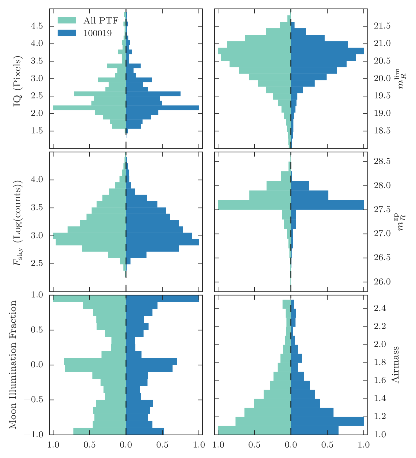
Figure 1: The (renormalized) distributions of the image metadata and observing conditions (Section 2.1) across the entire PTF survey (left, light-shaded histograms) compared to those of the PTF field 100019 used in our recovery efficiency simulations (right, dark-shaded histograms). The top left panel shows the comparison for the image quality (IQ), the top right panel the limiting magnitude ($m_{R}^{\mathrm{lim}}$), the center left panel the median sky counts ($F_{\mathrm{sky}}$), the center right panel the photometric zeropoint ($m_{R}^{\mathrm{zp}}$), the lower left panel the moon illumination fraction (0 = new moon, -1,1 = full moon), and the lower right the airmass of the observation.

2.2.1 Selecting point sources

Our fakes are sampled from real point-sources located in each image. We use sextractor to locate the 20 brightest, unsaturated, and isolated point sources (i.e., ‘stars’), ensuring each is $>50$ pixels from the CCD edge. Our selection is based on the sextractor neural network class_star classifier, which assigns every object a value from 0 (not star-like) to 1 (star-like). This cut removes galaxies and cosmic rays from our fakes catalog, which we confirmed by visual inspection from a random sample of 1084 candidate stars. We do note, however, that a small fraction of the visually inspected stars show some ‘blooming’ into adjacent pixels. This contamination is difficult to filter out as these stars still receive a high class_star value in sextractor. For our selected stars sources, 99.5% of the objects have a class_star score >0.92.

Our fakes are then constructed by ‘clone-stamping’ these bright stars: we take a box of 9 pixels on a side that encloses the PSF, subtract the local sextractor background, and re-scale the star to the desired fake apparent magnitude ($m_{R}$). This method ensures that the fakes have a PSF that is both representative of real objects in the image, but also carries the intrinsic variation of the PSF (the object-to-object variation) within the simulation. We generate fakes with a uniform magnitude distribution from $m_{R}$=15–22 mag. We additionally enforce the condition that each fake must be a least one magnitude fainter than the original star from which it was generated.

2.2.2 Inserting fakes into the data

A key consideration when inserting the fakes into the PTF data is that the presence of these ‘extra’ sources does not distort the machine learning classification process. One of the 28 metrics (Bloom et al., 2012) that goes into the RB score is the spatial density of good candidates, defined as the ‘ratio of the number of candidates in that subtraction to the total usable area on that array’. Thus, saturating an image with an artificially high density of fakes may lead to unrepresentative RB scores. A secondary effect is that adding too many fakes into an image could affect the astrometric alignment of the science image to the reference, and thus cause an increased number of subtraction artefacts.

We therefore investigated, using a random sample of 281 images made available to us for pipeline development from the tape archives, how the addition of fakes changed the RB scores of real candidates in the images. In Figure 2, we compare our baseline RB scores of real candidates (when there are no fakes in an image) with the RB scores of the same candidates but with an increasing number of fakes added. We find that even a small number of fake objects slightly distorts the RB scores; however these effects remains negligible when of order tens of fakes are added, only becoming important with $>$100 fakes. Based on our analysis, we consider 60 fake objects per image to be a satisfactory compromise between maximizing our computational efficiency and distorting the RB scores. We also note that even with 400 fakes per image, the astrometric alignment to the reference image was not changed.

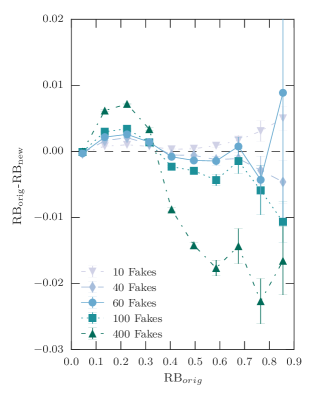
Figure 2: The original Real-Bogus (RB; Section 2.1) scores (RB_orig) of the real candidate objects in our sample images, compared to the RB scores of the same objects with different numbers of fakes added to the same images (RB_new). The figure shows cases where 10, 40, 60, 100 and 400 fakes have been added to the images.

2.2.3 Fake Point Source locations

Most real astrophysical transient events occur within an associated host galaxy. However, if our fakes were added to random locations on the sky, then the majority would instead be placed in host-less regions, and consequently would provide poor statistics on the recovery efficiency as a function of host galaxy parameters, such as local surface brightness. This would require us to perform many more fake point-source simulations in order to adequately map this parameter space.

We therefore choose to bias the locations of our fakes to ensure that 90% of them are placed within a detected galaxy. To select a host for these fake point sources, the sextractor catalogs were used to randomly choose galaxies in each image, with the galaxy pixel positions given by ($x_{\mathrm{gal}}$, $y_{\mathrm{gal}}$). A fake is then added at a pixel position ($x_{\mathrm{SN}}$, $y_{\mathrm{SN}}$) at an elliptical radius $R$ within the isophotal limit of each galaxy. The elliptical shape parameters are measured by sextractor, defined by the semi-major ($r_{A}$) axis, the semi-minor ($r_{B}$) axis, and the position angle ($\theta$), with $R$ given by

$$R^{2}=C_{xx}(x_{\mathrm{SN}}-x_{\mathrm{gal}})^{2}+C_{yy}(y_{\mathrm{SN}}-y_{\mathrm{gal}})^{2}+\\ C_{xy}(x_{\mathrm{SN}}-x_{\mathrm{gal}})(y_{\mathrm{SN}}-y_{\mathrm{gal}})$$ (1)

where $C_{xx}=\cos^{2}(\theta)/r_{A}^{2}+\sin^{2}(\theta)/r_{B}^{2}$, $C_{yy}=\sin^{2}(\theta)/r_{A}^{2}+\cos^{2}(\theta)/r_{B}^{2}$, and $C_{xy}=2\cos(\theta)\sin(\theta)(1/r^{2}_{A}-1/r_{B}^{2})$. A value of $R\sim 3$ corresponds to the isophotal limit of each object. The location of each fake is not refined further, for example to follow a galaxy surface brightness profile. The remaining 10% of the fakes were added into blank regions of the sky. We also ensure that a fake is not within 40 pixels of another fake, regardless of whether it is in a galaxy or not.

2.3 Fake supernova recovery

The simulation method described above is applied 10 times to all observations of the PTF field 100019 taken over 2009–2012, generating a sample of $\approx$7$\times 10^{6}$ fakes in the data. The product of our simulations are two PostgreSQL database tables. The first stores a complete description of the parameters describing each fake: the spatial location and any host galaxy information, the fake magnitude, and the observing conditions metadata. The second table stores the output from the real-time detection pipeline run on the images containing the fakes, including the machine learning RB scores; i.e., it contains information on which fakes were recovered by the pipeline (as well as all the real astrophysical transients and false-positives).

To determine whether a fake was recovered by the pipeline, we perform a spatial matching of the two databases (fake positions versus recovered positions), and require that any matched fake must have a RB score $\geq 0.07$, the same as during the PTF survey operation (Bloom et al., 2012). The matching radius between a fake and a recovered candidate varies with the IQ (seeing), and to remove spurious associations we define $\Theta_{\mathrm{IQ}}$ as the ratio of the separation of a fake and the nearest recovered candidate, to the IQ. The histogram of all $\Theta_{\mathrm{IQ}}$ is shown in Figure 3, and we enforce $\Theta_{\mathrm{IQ}}<0.6$ in order to consider a fake to be recovered. Any fake without a detection satisfying $\mathrm{RB}\geq 0.07$ and $\Theta_{\mathrm{IQ}}<0.6$ is considered not recovered.

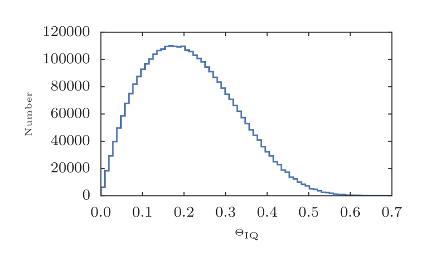
Figure 3: The distribution of $\Theta_{\mathrm{IQ}}$, where $\Theta_{\mathrm{IQ}}$ is defined as the separation between the position of the input fake and the position of the nearest recovered candidate, divided by the IQ of the image. We require that $\Theta_{\mathrm{IQ}}<0.6$ in order to consider a fake to be recovered by the pipeline.

2.4 Recovered fake point source properties

We next compare the recovered fake’s magnitude to that input into the pipeline (Figure 4). Although this is not a critical part of our analysis, as we do not use the recovered photometry in our analysis, this test acts as a useful sanity check that our efficiency pipeline is working as expected, and that the PTF real-time pipeline itself can recover reasonably accurate photometry. The agreement is generally good, and as expected, the fainter fake SNe show a larger scatter between their input and recovered magnitudes as the signal-to-noise (S/N) decreases; however the overall comparison shows a good agreement with no systematic offset. We find that 92% of the recovered fake magnitudes are within 0.2 mag of their input magnitudes, and splitting our fakes into bright objects ($m_{R}\leq 18.5$ mag) and fainter objects ($m_{R}>18.5$ mag) we find 98% and 77% of the magnitudes are recovered within 0.2 mag. Thus the PTF real-time search pipeline accurately recovers the input magnitudes of the fakes.

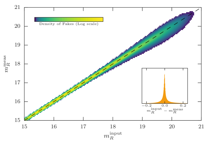
Figure 4: The sextractor measured magnitudes ($m_{R}^{\mathrm{meas}}$) for the recovered fakes compared to their input magnitudes ($m_{R}^{\mathrm{input}}$). The main panel shows the overall comparison with the dashed line denoting a 1:1 agreement, and the inset panel shows the distribution of $m_{R}^{\mathrm{meas}}-m_{R}^{\mathrm{input}}$ which is sharply peaked at 0 showing no systematic offset.

3 Recovery statistics

We now study the performance of the pipeline in recovering fakes under different observing conditions, and as a function of the input fake’s properties and location. We use this to motivate the construction of a multi-dimensional recovery efficiency grid as a function of the smallest number of parameters that affect the recovery of a fake. We can then use this multi-dimensional grid together with Monte Carlo simulations to calculate the recovery efficiency of real transient events.

3.1 Single parameter recovery efficiencies

We begin by binning the data based on the input fake properties and observing conditions with bin widths and number driven by the precision with which the data are measured. For example, the $m_{R}^{\mathrm{zp}}$ values are determined by the real-time pipeline to an accuracy of 0.1 mag, and so fewer, larger, bins are required compared to $m_{R}^{\mathrm{lim}}$, which is measured to a higher precision. The same binning is applied to the equivalent data associated with the fakes that are recovered by the PTF pipeline. We then define, in each bin $i$, the recovery efficiency $\epsilon_{i}$ to be the ratio of the number of fake objects recovered in each bin ($k_{i}$), to the total number of fakes originally created in that bin ($n_{i}$) i.e., $\epsilon_{i}=k_{i}/n_{i}$. One-dimensional recovery efficiencies for each variable are shown in Figure 5, in each case marginalized over the other variables.

An important question is the calculation of uncertainties for each $\epsilon_{i}$. In each bin, the number of successful detections of a fake is a binomially distributed variable, i.e., there are $k$ successes (detections) out of $n$ independent trials (fakes), which is expressed by

$$p(k|\epsilon,n)=\frac{n!}{k!(n-k)!}\epsilon^{k}(1-\epsilon)^{n-k}$$ (2)

where the probability of success on each trial is the efficiency $\epsilon$. For the frequentist approach, it can be straight-forwardly shown that $\sigma_{\epsilon}=\sqrt{k(n-k)/n^{3}}$ (Paterno, 2004); however this equation fails in the limiting cases of $k=0$ or $k=n$. Instead, we use Bayes Theorem with Equation 2 to derive the posterior probability distribution of $\epsilon$

$$p(\epsilon|k,n)=\frac{\Gamma(n+2)}{\Gamma(k+1)\Gamma(n-k+1)}\epsilon^{k}(1-\epsilon)^{n-k}$$ (3)

with a uniform prior in $\epsilon$ that $0\leq\epsilon\leq 1$, where $\Gamma$ is the Euler gamma function; see Paterno (2004) for details. Uncertainties are then calculated by numerically finding the shortest interval containing 68.3% of the probability.

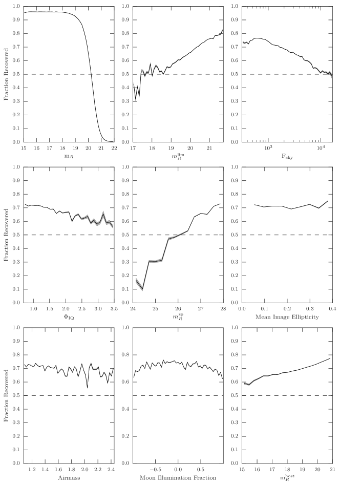
Figure 5: The fake recovery efficiency $\epsilon$ as a function of 8 of the variables we consider and the fake’s magnitude. In each individual panel, the recovery efficiencies are marginalized over the other parameters. These are (top row) the fake magnitude $m_{R}$, the limiting magnitude of the image $m_{R}^{\mathrm{lim}}$, the median sky counts in the image $F_{\mathrm{sky}}$, the ratio of the seeing in the science and reference images, the image photometric zeropoint $m_{R}^{\mathrm{zp}}$, the mean image ellipticity, the airmass of the observation, the moon illumination fraction at the observing epoch and the host galaxy magnitude for the fake $m_{R}^{\mathrm{host}}$. The dashed lines represent the points at which 50% of the fakes are recovered and the shaded regions contain 68.3% of the probability.

Several clear (and expected) trends are apparent in Figure 5; for example fake objects are more difficult to recover when fainter. However, even when the fake is bright ($m_{R}<18.5$ mag), we note that a consistent $\approx 3$% of objects are not recovered, implying that some small fraction of objects are missed no matter what the brightness. Fake objects are also more difficult to recover as the IQ of the science image becomes poorer relative to that of the reference image; as the limiting magnitude becomes brighter; and as the photometric zeropoint becomes brighter (i.e., the data have more attenuation, presumably from clouds). The recovery fraction is also a strong function of median sky counts (a brighter sky makes the fake harder to detect), a weak function of the moon illumination fraction (objects are harder to recover with a bright moon), and a weak function of airmass (objects are marginally more difficult to recover at high airmass). There is no measurable trend with image ellipticity, indicating the image subtraction works well across most PTF data.

3.1.1 Host galaxy surface brightness

As the fakes were inserted (see Section 2.2.3), we record the total integrated $R$-band apparent magnitude of any host galaxy ($m_{R}^{\mathrm{host}}$) from the sextractor catalog, as well as the local surface brightness at the position of the fake. We denote this latter parameter ‘$F_{\mathrm{box}}$’, defined as the background-subtracted sum of the pixel counts at the fake position over different configurations of pixels. We record this metric in box sizes from 1$\times$1 to 11$\times$11 pixels, however our default for all $F_{\mathrm{box}}$ measures is to use the integrated counts in a 3$\times$3 box as this is close in size to the PSF of a typical fake. This metric provides local environment information for an object’s recovery efficiency, i.e., the transient detection pipeline’s ability to discover sources against a bright background. The $F_{\mathrm{box}}$ metric is the only parameter we discuss that was not output from the from the real-time pipeline during survey operations between 2009-2012. Thus any study based on the results of our efficiencies, which explicitly require the use of $F_{\mathrm{box}}$, will need to measure $F_{\mathrm{box}}$ for their transient objects so that they are directly comparable to our fake simulations. The real-time pipeline did measure a fixed aperture flux of 5 pixels in both the subtraction and the reference, referred to as the flux-ratio in Bloom et al. (2012). However, while useful for computing the real-bogus score, we found it insufficient for our needs as it was in general too large compared to the typical PSF.

Figure 5 shows that fakes become more difficult to recover in brighter galaxies. However, $m_{R}^{\mathrm{host}}$ is a poor choice of metric shown only for information. It is not applicable to all real transient events (where the host association may be uncertain; e.g., Sullivan et al., 2006; Gupta et al., 2016), and can be mis-leading if, say, a transient is well-separated from a bright host galaxy. Instead, the information is more usefully encapsulated by the $F_{\mathrm{box}}$ metric. In Figure 6 (left) we inspect the recovery efficiency as a function of $F_{\mathrm{box}}$  split into bins of fake magnitude, and see the expected trend where fakes in regions of higher surface brightness are less likely to be recovered. We also extend this analysis to a new parameter, $\vartheta_{\mathrm{ratio}}$: the ratio $F_{\mathrm{box}}$ to the flux from the fake. This new parameter, when considered alone, provides an insight into how cleanly the image subtraction has been performed, which can particularly affect the fainter fakes on bright galaxies. We note that $\vartheta_{\mathrm{ratio}}$ has a degeneracy with $m_{R}$ (as both include the counts from the fake) and in Section 3.2 we do not use $m_{R}$ in conjunction with $\vartheta_{\mathrm{ratio}}$ for this reason.

In Figure 6 (right) we examine the recovered fraction of fakes as a function of $\vartheta_{\mathrm{ratio}}$. We find the expected trend where fakes that are located in an environment of high surface brightness relative to the object itself are less likely to have been detected by the pipeline. The pipeline maintains a consistently high ability to discover the fakes whilst the fakes are $\approx$10$\times$ brighter than $F_{\mathrm{box}}$. The recovered fraction rapidly drops off after this point, with 50% recovered at $\vartheta_{\mathrm{ratio}}$$\approx 0.7$

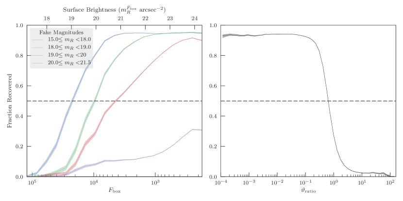
Figure 6: Left: The recovery efficiency as a function of the $F_{\mathrm{box}}$ parameter on the bottom axis and $m_{R}^{F_{\mathrm{box}}}$ surface brightness on the top axis. We see the expected trend of fewer fakes recovered when they are situated in bright regions (analogous to bright host galaxies). Right: The recovery efficiency as a function of the ratio of counts in $F_{\mathrm{box}}$ to the counts of the fake point source ($\vartheta_{\mathrm{ratio}}$). We find that if the local surface brightness is $\lesssim$0.1$\times$ than the fake, the pipeline finds it $\approx$95% of the time. Beyond this the recovered fraction sharply falls off and the 50% recovery fraction is at $\vartheta_{\mathrm{ratio}}$$\approx$10^-0.2

3.1.2 Efficiencies as a function of time

Due to the improvement and updating of the reference images during the survey (Section 2.1), we expect the recovery efficiencies to show a time dependence. We therefore plot the recovery efficiencies as a function of $m_{R}$ for each year of the survey (Figure 7), and find that 2009 has a significantly lower recovery efficiency than the subsequent years. The later years – 2010, 2011, 2012 – all show consistent trends. Given the large discrepancy between 2009 and the later years, we exclude 2009 from our study. While the effect in 2009 is partly explainable due to the likely lower quality of the references during 2009 (both in terms of depth and IQ), we also note that the data from 2009 suffered from a ‘fogging’ problem on the PTF camera window (described in detail in Ofek et al., 2012). This likely dramatically decreased the efficiency of the survey in the parts of the image affected by the fogging during that period.

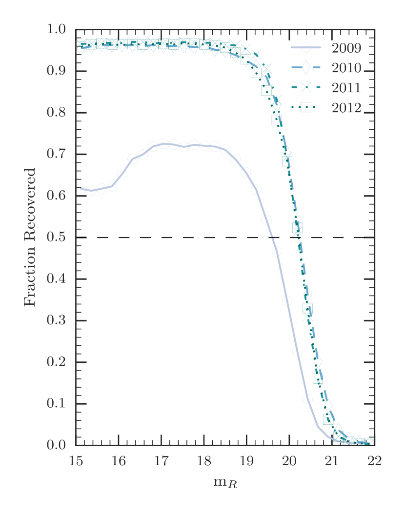
Figure 7: The recovery efficiency as a function of fake apparent magnitude ($m_{R}$) for each year of the PTF survey (averaged over all observing conditions). The years 2010–2012 are consistent, but the year 2009 (the first year of the PTF survey) shows a large discrepancy (see discussion in section 3.1). We exclude 2009 from our analysis.

3.1.3 50% recovery efficiencies

The 50% recovery magnitude $m_{R}^{50}$ – the magnitude at which PTF finds the same number of transients as it misses – is another useful way of parameterizing the survey efficiencies. Taken over all observing conditions, $m_{R}^{50}\approx 20.3$ mag (Figure 5). However, $m_{R}^{50}$ depends strongly on the observing conditions and galaxy surface brightness. We show $m_{R}^{50}$ as a function of $m_{R}^{\mathrm{lim}}$, $F_{\mathrm{sky}}$, $\Phi_{\mathrm{IQ}}$  $m_{R}^{\mathrm{zp}}$, airmass and moon illumination fraction parameters in Figure 8; the trends are as expected.

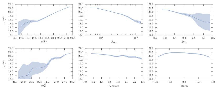
Figure 8: The 50% recovery magnitude, $m_{R}^{50}$, as a function of various observing conditions. The results are plotted on the same axis scale to highlight the negligible dependence of these parameters in shifting the recovery efficiencies which is explained further in Section 3.2. The shaded areas indicate the statistical uncertainties (containing 68.3% of the probability).

3.2 Multidimensional recovery efficiencies

We now extend our analysis of the single parameter recovery fractions to study PTF’s performance as a function of multiple variables – our final recovery efficiency grid. This method allows for situations to be studied which cannot be encapsulated by any single parameter, for example bright transients occurring in poor observing conditions. It is possible to create a multi-dimensional efficiency grid from all of the parameters discussed in Section 3.1 and shown in Figure 5; however, several of these variables are likely to encapsulate similar information, and are therefore may be degenerate (the correlations are given in Figure 9). For computational reasons, it is more efficient to construct a final recovery efficiency grid composed of the fewest dimensions possible, but which capture the great majority of the variation. In this section, we therefore examine the most important variables that will make up a final efficiency grid. We stress that whilst we aim to reduce the number of dimensions to produce a final efficiency grid applicable for most purposes, there is flexibility in this method to include any number of parameters to meet the specific science goals of a study.

Figure 9: The correlation matrix for the observational metadata we record in our database. We explore the inter-dependencies of the parameters so that the number of dimensions in the final efficiency grid can be minimized to exclude strongly correlated parameters where no new information is gained. The values in each of the cells are the Pearson correlation coefficients.

The first dimension of our final efficiency grid is the apparent magnitude of the fake object ($m_{R}$), a variable that is clearly essential. the second dimension is $F_{\mathrm{box}}$, again containing information not captured by the other variables. The remaining dimensions are then drawn from the observing conditions. In Figure 9, we explore the Pearson correlation coefficients for the 6 pieces of recorded metadata listed in Section 2.1; we neglect the image ellipticity, as it has little impact on the efficiencies (Figure 5). We then construct, in Figure 10, the 6-dimensional grid of efficiencies where each cell in the grid is the probability of recovering a transient as a combination of these 6 observing conditions. These parameters are binned in an identical way to the one-dimensional efficiencies as described in Section 3.1, but with the absolute value of moon illumination fraction.

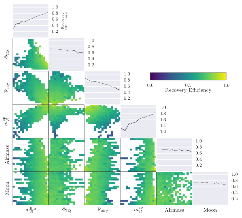
Figure 10: The 6-dimensional grid of the observing conditions metadata. The diagonal elements are the 1-dimensional recovery efficiencies $\epsilon$, projected along the axis of interest, with the gray shading denoting the area containing 68.3% of the probability in $\epsilon$. The off-diagonal elements represent the different combinations of all the parameters.

To find the remaining dimensions with the most power, we weight each multi-dimensional element in the grid by the inverse of the 1-dimensional detection efficiency associated with that bin for the parameter we are interested in. We then assess the remaining 1-dimensional projections for indications of residual trends in efficiency that would indicate that there is information in that axis that was not also contained in the parameter used for the weighting. We extend this analysis to combinations of weighted dimensions, and, after experimentation, find from Figure 11 that we remove residual efficiency trends with $m_{R}^{\mathrm{zp}}$, airmass and moon illumination fraction when re-weighting the efficiency grid using the $m_{R}^{\mathrm{lim}}$, $\Phi_{\mathrm{IQ}}$, and $F_{\mathrm{sky}}$ parameters. (Note some residual trends remain with $m_{R}^{\mathrm{zp}}$, but only at the extremes of the distribution representing poor observing conditions, presumably cloudy).

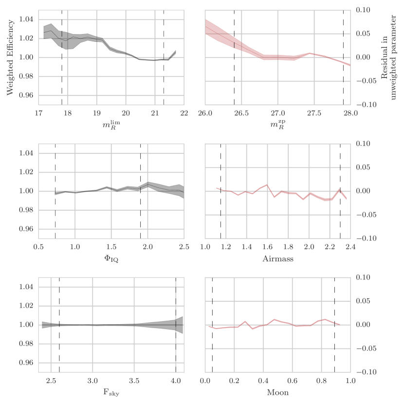
Figure 11: We explore which dimensions of the efficiency grid contain the most information. We show that by re-weighting the $m_{R}^{\mathrm{lim}}$, $\Phi_{\mathrm{IQ}}$ and $F_{\mathrm{sky}}$ axis (left column), we can remove the efficiency trends in the $m_{R}^{\mathrm{zp}}$, airmass and $\left|\mathrm{moon\ illumination\ fraction}\right|$ axes. We show this by plotting the residuals from a perfect recovery efficiency (right column). The dashed vertical lines represent bounds containing 99% of the data.

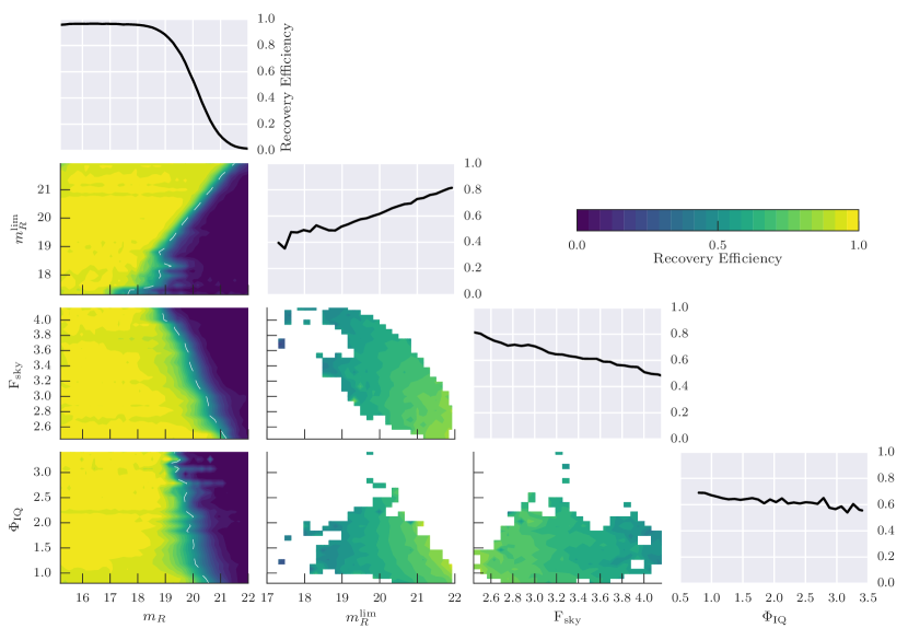
Figure 12: The final multi-dimensional efficiency grid. The off diagonal entries show the two dimensional efficiencies for combinations of the parameters. The diagonal entries show the one dimensional recovery efficiencies created by marginalizing other the other grid parameters. The white dashed lines on the $m_{R}$ axis denote the 50% recovery efficiency for this parameter against the other observing condition parameters.

Thus, the bulk of the variation in efficiency is captured by the 5 parameters of $m_{R}$, $F_{\mathrm{box}}$, $m_{R}^{\mathrm{lim}}$, $\Phi_{\mathrm{IQ}}$, and $F_{\mathrm{sky}}$, and the final recovery efficiency grid is comprised of these variables (Figure 12). The reduced dimensionality of this final grid also allows a finer binning of the data, increasing the resolution. The grid can then be used to estimate the recovery efficiency of a point source observed under any PTF observing conditions. This probability of a detection, given $m_{R}$, $F_{\mathrm{box}}$, $m_{R}^{\mathrm{lim}}$, $F_{\mathrm{sky}}$, and $\Phi_{\mathrm{IQ}}$, is calculated using a linear interpolation on the final efficiency grid.

4 Simulating PTF for a transient population

We have constructed a multi-dimensional recovery efficiency grid for the PTF survey for transient point sources, describing the recovery efficiency as a function of various astrophysical and observational parameters. This allows us to calculate the fraction of point sources recovered on any epoch or image from PTF as a function of the point source magnitude $m_{R}$ and the host galaxy background. In this section, we briefly describe how such an efficiency grid can be applied to a real astrophysical problem; for example for calculating the rates of particular types of transient events. We do this, in effect, by simulating an artificial ‘night sky’ across the PTF survey area populated by transients defined by a time-dependent luminosity model, and then exactly replicate PTF’s observing pattern to observe this artificial sky. Using the PTF metadata for each observation and the efficiency grid from Section 3.2, we can then determine which of these simulated transients would have been recovered.

Over the course of PTF, thousands of fields were observed across an approximate footprint of $8000$ deg². We initially explored treating each PTF field as its own distinct area in which to simulate transients. However, we found that this would underestimate our calculation of the transient discovery efficiency as the PTF fields spatially overlap, by design, and dither very slightly due to imperfect telescope pointing. A transient event occurring in one of the overlap regions would then be sampled more frequently under real conditions than in the simulations, increasing the likelihood of discovery and light curve coverage.

It is therefore simpler to treat the entire PTF survey as one single field, simulating transients at random positions within this field and with random explosion epochs. We use the PTF database to determine on which CCD (if any) the object would have been observed and the observing conditions for that CCD. These, along with the transient apparent magnitude, are used to interpolate on the multi-dimensional efficiency grid from Section 3.2, to give the likelihood of recovering the transient on that epoch.

To determine whether a transient is observed on a given CCD, we use the geospatial table extender PostGIS. Each CCD is projected onto a spherical surface based on the RA and Dec. of the corner pixels, and the geospatial location information is stored and indexed in a new table along with the other PTF observational metrics. The RA and Dec. of the simulated transient are the query arguments which returns all CCDs which enclose that point. With over 1.6$\times 10^{6}$ observations taken throughout the survey, this method allows us to retrieve all the CCDs, together with their observing conditions, for a specific RA, Dec., and JD range, within $\backsimeq 0.01$ s.

4.1 Simulating a transient population

A transient population can be constructed from a time-dependent luminosity model and inserted into our artificial sky, and the efficiency grid then used to derive the probability that PTF would have discovered it. In this section we demonstrate this technique on a particular type of transient, type Ia supernovae (SNe Ia), a supernova class with a well-defined light curve model. Note that here we are simply demonstrating how the efficiency grid may be used; we apply our efficiency grid to a real SN Ia rates calculation in a later article.

The key to the method is to build up a second efficiency grid with its axes made up of variables that describe the transient being simulated, and that can be measured for real events. For this demonstration, we use the SALT2 SN Ia model (Guy et al., 2007) within the Python package sncosmo (Barbary, 2014) to generate the SN Ia light curves. Our algorithm allows us to Monte Carlo variations of the model and place them within the PTF survey at different epochs and locations on the night sky. The model generates a spectral energy distribution (SED) time series for a SN Ia, converted into flux- or magnitude-space by integrating the SED through the filter response of the $R_{\mathrm{P48}}$ filter.

For this demonstration, the key parameters are the light curve shape (the $x_{1}$ parameter, analogous to a light curve ‘stretch’; see Perlmutter et al., 1997; Guy et al., 2007) and the color ($c$, which represents the B V color of the SN at the time of maximum light). Each simulated event also requires a spatial position and epoch of explosion. To calculate the absolute magnitude of each event, $M_{B}$, we randomly generate parameters from each SN Ia ($x_{1}$, $c$, $z$, $\sigma_{\mathrm{int}}$) according to the distributions in Table 1 and insert them into

$$M_{B}=-19.05-\alpha x_{1}+\beta C+\sigma_{\mathrm{int}}.$$ (4)

where $\alpha$ and $\beta$ are ‘nuisance parameters’ defining the $x_{1}$–luminosity and color–luminosity relations, $-19.05$ is the absolute magnitude for a typical SN Ia, and $\sigma_{\mathrm{int}}$ is the intrinsic dispersion of each event, capturing the intrinsic brightness variation in the SN Ia population after light curve shape and color correction. We use $\alpha=0.141$ and $\beta=3.101$ for this demonstration, following Betoule et al. (2014). We then use the redshift $z$ to calculate the distance modulus to transform to an apparent magnitude in the observed $R_{\mathrm{P48}}$ filter, including Milky Way extinction according to the chosen spatial location on the sky.

Table 1: SALT2 SN Ia model parameters used in the simulation.

Parameter	Distribution	Range
$x_{1}$	Uniform	-3.0 to 3.0
Color ($c$)	Uniform	-0.3 to 0.3
Intrinsic dispersion ($\sigma_{\mathrm{int}}$)	Normal	$\mu=0,\sigma=0.15$
Redshift ($z$)	Uniform	0.0 to 0.1

This model then provides a light curve at a specific RA and Dec. on our artificial night sky. A spatial query of the PTF database returns all the observing metrics for any CCD that could have observed the SN, and the SN model gives the apparent magnitude for each of these observing epochs. This observed magnitude is then used together with the observing metadata to perform a multidimensional linear interpolation on the efficiency grid described in Section 2, returning the probability of PTF detecting the object on each observed epoch ($P_{\mathrm{detect}}$). For each epoch, we then randomly select a number, $\lambda$, from a uniform distribution between 0 and 1 for comparison with that epoch’s detection probability: if $\lambda\leq P_{\mathrm{detect}}$, the SN is considered detected on that epoch, and if $\lambda>P_{\mathrm{detect}}$ the SN is considered not detected. Figure 13 demonstrates this concept, showing typical observational metric locations on the efficiency grid for a demonstration SN Ia.

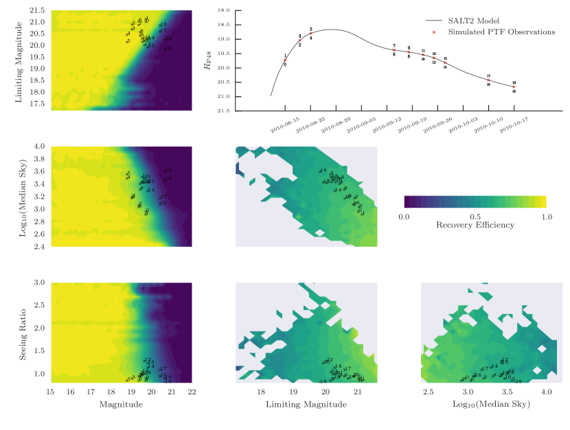
Figure 13: A demonstration of the implementation of our detection efficiency grid for an example transient. The light curve model (in this case for a SN Ia) is used to predict the apparent magnitude on every epoch on which PTF made an observation of the spatial position of the model event (top right panel) and the PTF database returns the observing conditions on that epoch. Each combination of apparent magnitude and observing conditions then has an associated efficiency $P_{\mathrm{detect}}$, interpolated from the multi-dimensional efficiency grid; the figure shows the position of the point in various combinations of the grid dimensions, and the points are numerically labeled in the figure (PTF typically observes each position twice during a given night). If the value of $P_{\mathrm{detect}}$ is greater than or equal to a random number between 0 and 1, then that point is considered detected by PTF; otherwise the point is not considered detected. This process is repeated for each observation. The entire light curve can then be considered against appropriate selection criteria that determine the probability of whether the transient would be detected over the course of its evolution.

To construct recovery efficiencies as a function of the SN parameters, we then construct a grid with the simulated SN parameters as the axes of the grid (in this case $z$, $x_{1}$, $c$, $\sigma_{\mathrm{int}}$). By simulating millions of fake SNe in the PTF area, simulated with parameters drawn from the distributions in Table 1 and assessing whether each would have been recovered by PTF, we can then populate this grid. The recovery efficiency $\epsilon_{\mathrm{SN}}$ of a real SN can then be estimated by interpolating on this grid at the position of the values that represent the real SN. For example, if a real supernova is found to have $\epsilon_{\mathrm{SN}}=0.2$ from the simulated sky area, then it means that this one object represents a population of five, where the other four were missed by the survey.

Our method of simulating transients on an artificial sky and then ‘observing’ it encodes two pieces of information into the $\epsilon_{\mathrm{SN}}$ metric. The first is an efficiency that is intrinsically linked to the supernova model parameters. The second is the sky area of the simulation; that is, the $\epsilon_{\mathrm{SN}}$ are calculated for an area of sky that may be larger than the area actually observed, which must be borne in mind when interpreting the $\epsilon_{\mathrm{SN}}$ values.

5 Summary

This paper has presented the transient detection efficiencies for the Palomar Transient Factory (PTF). These efficiencies were quantified through the addition of fake events into real PTF images, which were then run through PTF’s real-time transient detection pipeline. The fraction of these fake transients recovered by the PTF pipeline then quantifies the performance of PTF across a variety of observing conditions, and transient magnitudes and local environments. This information is captured in the form of a multi-dimensional efficiency grid, which can then be used, together with Monte Carlo simulations of transient events, to calculate rates and luminosity functions of different transient types. We will detail these studies in later articles.

References

- Baltay et al. (2013) Baltay, C., Rabinowitz, D., Hadjiyska, E., et al. 2013, PASP, 125, 683
- Barbary (2014) Barbary, K. 2014, sncosmo v0.4.2, , , doi:10.5281/zenodo.11938
- Bertin (2006) Bertin, E. 2006, in Astronomical Society of the Pacific Conference Series, Vol. 351, Astronomical Data Analysis Software and Systems XV, ed. C. Gabriel, C. Arviset, D. Ponz, & S. Enrique, 112
- Bertin & Arnouts (1996) Bertin, E., & Arnouts, S. 1996, A&AS, 117, 393
- Bertin et al. (2002) Bertin, E., Mellier, Y., Radovich, M., et al. 2002, in Astronomical Society of the Pacific Conference Series, Vol. 281, Astronomical Data Analysis Software and Systems XI, ed. D. A. Bohlender, D. Durand, & T. H. Handley, 228
- Betoule et al. (2014) Betoule, M., Kessler, R., Guy, J., et al. 2014, A&A, 568, A22
- Bloom et al. (2012) Bloom, J. S., Richards, J. W., Nugent, P. E., et al. 2012, PASP, 124, 1175
- Cao et al. (2016) Cao, Y., Nugent, P. E., & Kasliwal, M. M. 2016, PASP, 128, 114502
- Drake et al. (2009) Drake, A. J., Djorgovski, S. G., Mahabal, A., et al. 2009, ApJ, 696, 870
- Gupta et al. (2016) Gupta, R. R., Kuhlmann, S., Kovacs, E., et al. 2016, ArXiv e-prints, arXiv:1604.06138
- Guy et al. (2007) Guy, J., Astier, P., Baumont, S., et al. 2007, A&A, 466, 11
- Kaiser et al. (2010) Kaiser, N., Burgett, W., Chambers, K., et al. 2010, in Proc. SPIE, Vol. 7733, Ground-based and Airborne Telescopes III, 77330E
- Kasliwal (2012) Kasliwal, M. M. 2012, PASA, 29, 482
- Kessler et al. (2015) Kessler, R., Marriner, J., Childress, M., et al. 2015, AJ, 150, 172
- Law et al. (2009) Law, N. M., Kulkarni, S. R., Dekany, R. G., et al. 2009, PASP, 121, 1395
- Maguire et al. (2014) Maguire, K., Sullivan, M., Pan, Y.-C., et al. 2014, MNRAS, 444, 3258
- Monet et al. (2003) Monet, D. G., Levine, S. E., Canzian, B., et al. 2003, AJ, 125, 984
- Nugent et al. (2015) Nugent, P., Cao, Y., & Kasliwal, M. 2015, in Proc. SPIE, Vol. 9397, Visualization and Data Analysis 2015, ed. D. L. Kao, M. C. Hao, M. A. Livingston, & T. Wischgoll, 939702
- Nugent et al. (2011) Nugent, P. E., Sullivan, M., Cenko, S. B., et al. 2011, Nature, 480, 344
- Ofek et al. (2012) Ofek, E. O., Laher, R., Law, N., et al. 2012, PASP, 124, 62
- Oke & Gunn (1983) Oke, J. B., & Gunn, J. E. 1983, ApJ, 266, 713
- Pain et al. (2002) Pain, R., Fabbro, S., Sullivan, M., et al. 2002, ApJ, 577, 120
- Paterno (2004) Paterno, M. 2004, Calculating Efficiencies and Their Uncertainties, Tech. Rep. FERMILAB-TM-2286-CD, Fermilab
- Perlmutter et al. (1997) Perlmutter, S., Gabi, S., Goldhaber, G., et al. 1997, ApJ, 483, 565
- Perrett et al. (2010) Perrett, K., Balam, D., Sullivan, M., et al. 2010, AJ, 140, 518
- Rau et al. (2009) Rau, A., Kulkarni, S. R., Law, N. M., et al. 2009, PASP, 121, 1334
- Rubin et al. (2016) Rubin, A., Gal-Yam, A., De Cia, A., et al. 2016, ApJ, 820, 33
- Sako et al. (2008) Sako, M., Bassett, B., Becker, A., et al. 2008, AJ, 135, 348
- Smartt et al. (2015) Smartt, S. J., Valenti, S., Fraser, M., et al. 2015, A&A, 579, A40
- Sullivan et al. (2006) Sullivan, M., Le Borgne, D., Pritchet, C. J., et al. 2006, ApJ, 648, 868
- White et al. (2015) White, C. J., Kasliwal, M. M., Nugent, P. E., et al. 2015, ApJ, 799, 52