Quantum non-equilibrium effects in rigidly-rotating thermal states

Abstract

Based on known analytic results, the thermal expectation value of the stress-energy tensor (SET) operator for the massless Dirac field is analysed from a hydrodynamic perspective. Key to this analysis is the Landau decomposition of the SET, with the aid of which we find terms which are not present in the ideal SET predicted by kinetic theory. Moreover, the quantum corrections become dominant in the vicinity of the speed of light surface (SOL). While rigidly-rotating thermal states cannot be constructed for the Klein-Gordon field, we perform a similar analysis at the level of quantum corrections previously reported in the literature and we show that the Landau frame is well-defined only when the system is enclosed inside a boundary located inside or on the SOL. We discuss the relevance of these results for accretion disks around rapidly-rotating pulsars.
©2017. This manuscript version is made available under the CC-BY-NC-ND 4.0 license http://creativecommons.org/licenses/by-nc-nd/4.0/.

1 Introduction

In relativistic fluid dynamics, global thermal equilibrium can be attained if the product $\beta u^{\mu}$ between the inverse local temperature $\beta$ and the four-velocity $u^{\mu}$ of the flow satisfies the Killing equation [1, 2, 3, 4, 5]. A special property of thermal equilibrium is that the stress-energy tensor (SET) $T^{\mu\nu}_{\rm eq}=(E+P)u^{\mu}u^{\nu}+Pg^{\mu\nu}$ corresponds to that of an ideal fluid of energy density $E$ and pressure $P$ [2, 6, 7, 8]. In this letter, we will show that a quantum field theory (QFT) computation of the SET for rigidly-rotating thermal states (RRTS) contains non-ideal terms, as well as corrections to $E$ which become important near the speed of light surface (SOL). We discuss the relevance of these corrections in the context of an astrophysical application.

2 Kinetic theory analysis

In space-times with axial symmetry, RRTS in thermal equilibrium can be described using the Killing vector corresponding to rotations about the $z$ axis, i.e., $\beta u=\beta_{0}(\partial_{t}+\Omega\partial_{\varphi})$, where $\Omega$ is the angular velocity of the rotating state [7]. On Minkowski space, the particle four-flow $N^{\mu}_{\rm eq}$ and stress-energy tensor $T^{\mu\nu}_{\rm eq}$ corresponding to RRTS are given by:

$$N^{\mu}_{\rm eq}=nu^{\mu},\qquad T^{\mu\nu}_{\rm eq}=(E+P)u^{\mu}u^{\nu}+Pg^{\mu\nu},$$ (1)

while $\beta$ and $u=u^{\mu}\partial_{\mu}$ are given by:

$$\beta=\gamma^{-1}\beta_{0},\qquad u=\gamma(\partial_{t}+\Omega\partial_{\varphi}),$$ (2)

where $\gamma$ is the Lorentz factor of a co-rotating observer at distance $\rho$ from the $z$ axis:

$$\gamma=\left(1-\rho^{2}\Omega^{2}\right)^{-1/2}.$$ (3)

The Killing vector $\beta u$ becomes null on the SOL, where $\rho\Omega\rightarrow 1$ and co-rotating observers travel at the speed of light. From Eq. (2), it can be seen that the temperature $\beta^{-1}$ diverges as the SOL is approached. The energy density $E$ for massless particles obeying Fermi-Dirac (F-D) and Bose-Einstein (B-E) statistics is given by [6]:

$$E_{\rm F-D}=\frac{7\pi^{2}\gamma^{4}}{60\beta_{0}^{4}},\qquad E_{\rm B-E}=\frac{\pi^{2}\gamma^{4}}{30\beta_{0}^{4}},$$ (4)

while $P=E/3$. Since $E$ and $P$ diverge as inverse powers of the distance to the SOL, RRTS are well-defined only up to the SOL. While such divergent states clearly cannot occur in nature, rigid rotation can be induced in astrophysical systems, such as accretion disks around rapidly-rotating neutron stars or magnetars, where the intense magnetic field can lock charged particles into rigid rotation. We investigate the role of quantum corrections in such systems in Sec. 6.

3 Stress-energy tensor decompositions

Before discussing the quantum analogue of Eqs. (4), the tools necessary to analyse the SET in out of equilibrium states must be introduced. The main difficulty comes due to the equivalence between mass and energy in special relativity, which makes the distinction between the velocity $u^{\mu}$ and the heat flux $q^{\mu}$ ambiguous. For a general (time-like) choice of $u^{\mu}$, $N^{\mu}$ can be decomposed as [10]:

$$N^{\mu}=nu^{\mu}+V^{\mu},$$ (5)

where $n=-u_{\mu}N^{\mu}$ and the flow of particles in the local rest frame (LRF) $V^{\mu}$ is given by:

$$V^{\mu}=\Delta^{\mu}{}_{\nu}N^{\nu}$$ (6)

In the above, $\Delta^{\mu\nu}=u^{\mu}u^{\nu}+g^{\mu\nu}$ is the projector on the hypersurface orthogonal to $u^{\mu}$. The decomposition of the SET reads:

$$T^{\mu\nu}=Eu^{\mu}u^{\nu}+(P+\overline{\omega})\Delta^{\mu\nu}+W^{\mu}u^{\nu}+W^{\nu}u^{\mu}+\pi^{\mu\nu},$$ (7)

where the dynamic pressure $\overline{\omega}$, flow of energy in the LRF $W^{\mu}$ and shear stress $\pi^{\mu\nu}$, together with $V^{\mu}$, represent non-equilibrium terms. The quantities on the right hand side of Eq. (7) can be obtained through:

$$E=u^{\mu}u^{\nu}T_{\mu\nu},\quad P+\overline{\omega}=\frac{1}{3}\Delta^{\mu\nu}T_{\mu\nu},\quad W^{\mu}=-\Delta^{\mu\nu}u^{\lambda}T_{\nu\lambda},$$

$$\pi^{\mu\nu}=\left(\Delta^{\mu\lambda}\Delta^{\nu\sigma}-\frac{1}{3}\Delta^{\mu\nu}\Delta^{\lambda\sigma}\right)T_{\lambda\sigma},$$ (8)

For a massless fluid, $\overline{\omega}=0$. The heat flux $q^{\mu}$ is defined as [10]:

$$q^{\mu}=W^{\mu}-\frac{E+P}{n}V^{\mu}.$$ (9)

In the Eckart (particle) frame [2, 8, 11], $u^{\mu}_{e}$ is defined as the unit vector parallel to $N^{\mu}$. Observers in the LRF of the Eckart frame see a flow of energy ($W^{\mu}_{e}=q^{\mu}_{e}$) and no flow of particles ($V^{\mu}_{e}=0$). Since $N^{\mu}$ cannot be obtained using the QFT approach considered in this paper, the Eckart velocity $u^{\mu}_{e}$ cannot be defined. Hence, we will not consider the Eckart frame further in this paper.

In the Landau (energy) frame [2, 8, 12], $u^{\mu}\equiv u^{\mu}_{L}$ is defined as the eigenvector of $T^{\mu}{}_{\nu}$ corresponding to the (real, positive) Landau energy density $E_{L}$:

$$T^{\mu}{}_{\nu}u_{L}^{\nu}=-E_{L}u_{L}^{\mu},$$ (10)

such that $W^{\mu}_{L}=0$, which implies that there is no energy flux in the LRF. Since $V^{\mu}_{L}=-\frac{n_{L}}{E_{L}+P_{L}}q^{\mu}_{L}$ is in general non-zero, an observer in the LRF of the Landau frame will detect a non-vanishing particle flux.

Finally, the $\beta$-frame (thermometer frame) for the case of rigid rotation is defined with respect to [4]:

$$u_{\beta}=\gamma(\partial_{t}+\Omega\partial_{\varphi}).$$ (11)

A special property of the $\beta$-frame is that the LRF temperature is highest compared to the temperature measured with respect to any other frame [4]. In general, $V_{\beta}^{\mu}$ and $W_{\beta}^{\mu}$ do not vanish, such that the $\beta$-frame is a mixed particle-energy frame [13]. Due to the simplicity of its construction, we will start the analysis of the quantum SET with respect to the $\beta$-frame.

4 Klein-Gordon field

We now analyse the construction of RRTS from a QFT perspective. A first surprise comes from the analysis of the RRTS of the Klein-Gordon field: in the unbounded Minkowski space, there exist modes which have a non-vanishing Minkowski energy $\omega$ (i.e., with respect to the static Hamiltonian $H_{s}=i\partial_{t}$), while their co-rotating energy $\widetilde{\omega}=\omega-\Omega m$, measured with respect to the rotating Hamiltonian $H_{r}=i(\partial_{t}+\Omega\partial_{\varphi})$, vanishes. For such modes, the Bose-Einstein density of states factor $(e^{\beta\widetilde{\omega}}-1)^{-1}$ diverges, yielding divergent thermal expectation values (t.e.v.s) at every point in the space-time [14, 15]. The kinetic theory result (4) is clearly unaffected by this vanishing co-rotating energy modes catastrophy. Indeed, the problematic modes are no longer present in the QFT formulation if the system is enclosed within a boundary placed inside or on the SOL [15, 16]. Furthermore, a recent perturbative QFT analysis allows the computation of quantum corrections to the kinetic theory SET [17], which we will analyse in detail in what follows. For completeness, we present an analysis of the connection between these perturbative results and the non-perturbative QFT approach in A.

Substituting the results in Table III of Ref. [17] into Eq. (34) in Ref. [17] yields the following $\beta$-frame (2) decomposition of the SET:

$$E_{\beta}=\frac{\pi^{2}\gamma^{4}}{30\beta_{0}^{4}}+\frac{\Omega^{2}\gamma^{6}}{36\beta_{0}^{2}},\qquad W_{\beta}=\frac{\Omega^{3}\gamma^{7}}{18\beta_{0}^{2}}\left(\rho^{2}\Omega\partial_{t}+\partial_{\varphi}\right),$$

$$\pi^{\mu\nu}_{\beta}=\frac{\Omega^{2}\gamma^{6}}{54\beta_{0}^{2}}\begin{pmatrix}\gamma^{2}-1&0&\Omega\gamma^{2}&0\\ 0&1&0&0\\ \Omega\gamma^{2}&0&\rho^{-2}\gamma^{2}&0\\ 0&0&0&-2\end{pmatrix},$$ (12)

where $\omega=\Omega\gamma^{2}\partial_{z}$, $a=\rho\Omega^{2}\gamma^{2}\partial_{\rho}$ and $\gamma=\beta_{0}^{2}\Omega^{3}\gamma^{3}(\rho^{2}\Omega\partial_{t}+\partial_{\varphi})$ were used in Eq. (34) of Ref. [17]. Compared to the kinetic theory result (1), the quantum SET contains non-vanishing contributions in the form of the non-ideal terms $W^{\mu}$ and $\pi^{\mu\nu}$. Moreover, the second term in $E_{\beta}$ (12) represents a correction to $E_{\rm B-E}$ (4) which becomes dominant in the vicinity of the SOL due to the $\gamma^{6}$ factor.

The construction of the Landau frame yields:

$$E_{L}= \frac{E_{\beta}}{3}-\frac{1}{2}\bm{\hat{W}}_{\beta}\cdot\bm{\pi}_{\beta}\cdot\bm{\hat{W}}_{\beta}+\sqrt{\left(\frac{2E_{\beta}}{3}+\frac{1}{2}\bm{\hat{W}}_{\beta}\cdot\bm{\pi}_{\beta}\cdot\bm{\hat{W}}_{\beta}\right)^{2}-W^{2}_{\beta}},$$ (13)

$$u_{L}^{\mu}= \sqrt{\frac{E_{L}+\frac{1}{3}E_{\beta}+\bm{\hat{W}}_{\beta}\cdot\bm{\pi}_{\beta}\cdot\bm{\hat{W}}_{\beta}}{2(E_{L}-\frac{1}{3}E_{\beta}+\frac{1}{2}\bm{\hat{W}}_{\beta}\cdot\bm{\pi}_{\beta}\cdot\bm{\hat{W}}_{\beta})}}$$

$$\times\left(u_{\beta}^{\mu}+\frac{W_{\beta}^{\mu}}{E_{L}+\frac{1}{3}E_{\beta}+\bm{\hat{W}}_{\beta}\cdot\bm{\pi}_{\beta}\cdot\bm{\hat{W}}_{\beta}}\right),$$ (14)

where $W_{\beta}^{2}=\rho^{2}\Omega^{6}\gamma^{12}/324\beta_{0}^{4}\geq 0$, $\bm{\hat{W}}_{\beta}\equiv W_{\beta}/\sqrt{W_{\beta}^{2}}$ and $\bm{\hat{W}}_{\beta}\cdot\bm{\pi}_{\beta}\cdot\bm{\hat{W}}_{\beta}=\Omega^{2}\gamma^{6}/54\beta_{0}^{2}$. Surprinsingly, the Landau frame is well-defined only for $0\leq\rho\Omega\leq(\rho\Omega)_{\rm lim}$, where

$$(\rho\Omega)_{\rm lim}=\sqrt{x^{2}+x+1}-x,\qquad x=\frac{5}{4\pi^{2}}(\beta_{0}\Omega)^{2}.$$ (15)

When $\rho\Omega>(\rho\Omega)_{\rm lim}$, $E_{L}$ is no longer real. It can be seen that $(\rho\Omega)_{\rm lim}$ decreases from $1$ at $\beta_{0}\Omega=0$ (large temperatures or slow rotation) down to $0.5$ as $\beta_{0}\Omega\rightarrow\infty$.

We are again forced to regard the RRTS of the Klein-Gordon field as ill-defined. The natural question to ask is whether the problem with defining the Landau frame persists when the system is enclosed inside a boundary. Following Ref. [15], we construct the Landau frame for the case when the system is enclosed inside a cylinder of radius $R=\Omega^{-1}$ (i.e. placed on the SOL), on which Dirichlet boundary conditions are imposed. Fig. 1 shows that the Landau frame is well defined arbitrarily close to the boundary, where the Landau velocity $v_{L}=\rho u_{L}^{\varphi}/u_{L}^{0}$ decreases to $0$ due to the boundary conditions. It can also be seen in Fig. 1 that both $v_{L}$ and $E_{L}$ increase monotonically as $\beta_{0}$ is increased. Figure 1(b) also shows $E_{L}$ for the unbounded Minkowski space (13) for the case when $\beta_{0}\Omega=1$. The curve is interrupted at $\rho\Omega\simeq 0.942$, where $E_{L}$ becomes complex.

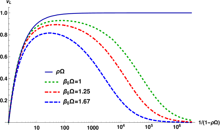
(a)

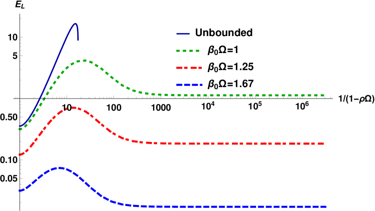
(b)

Figure 1: (a) Landau velocity $v_{L}=\rho u_{L}^{\varphi}/u_{L}^{0}$ and (b) Landau energy $E_{L}$ for massless Klein-Gordon particles enclosed inside a cylinder located on the SOL ($R=\Omega^{-1}$). The continuous curve in (a) shows the velocity $\rho\Omega$ for the case of rigid rotation, while in (b) it corresponds to the Landau energy (13) in the unbounded case. This curve is interrupted when $E_{L}$ becomes complex and the Landau frame is no longer well-defined.

5 Dirac field

The QFT analysis of the RRTS of the Dirac field is presented in Ref. [14]. The $\beta$-frame decomposition can be performed using $u_{\beta}$ (2) for the components of the SET given in Eqs. (25c)–(25f) in Ref. [14], yielding:

$$E_{\beta}= \frac{7\pi^{2}\gamma^{4}}{60\beta_{0}^{4}}+\frac{\Omega^{2}}{24\beta_{0}^{2}}\left(4\gamma^{6}-\gamma^{4}\right),$$ (16a)

$$W_{\beta}= \frac{\Omega^{3}\gamma^{7}}{18\beta_{0}^{2}}(\rho^{2}\Omega\partial_{t}+\partial_{\varphi}),$$ (16b)

while $P_{\beta}=E_{\beta}/3$ and $\pi_{\beta}^{\mu\nu}=0$. It is remarkable that $W^{\mu}_{\beta}$ for the Dirac field (16b) has the same expression as that for the Klein-Gordon field (12). As in the case of the Klein-Gordon field, the first term in Eq. (16a) corresponds to $E_{\rm F-D}$ (4), while the second term represents a quantum correction which dominates in the vicinity of the SOL. Figure 2(a) demonstrates this behaviour and it can be seen that the correction increases when either $\Omega$ or $\beta$ are increased.

The eigenvalue equation (10) can be solved analytically in terms of the Landau energy and velocity:

$$E_{L}= \frac{E_{\beta}}{3}+\sqrt{\frac{4E_{\beta}^{2}}{9}-W_{\beta}^{2}},$$ (17)

$$u_{L}^{\mu}= \sqrt{\frac{3E_{L}+E_{\beta}}{2(3E_{L}-E_{\beta})}}\left(u_{\beta}^{\mu}+\frac{3W_{\beta}^{\mu}}{3E_{L}+E_{\beta}}\right).$$ (18)

In contrast to the case of the Klein-Gordon field, the Landau frame is well-defined everywhere inside the SOL, since $4E_{\beta}^{2}/9W_{\beta}^{2}>1$ when $\rho\Omega<1$. The ratio $E_{L}/E_{\beta}$ decreases from $1$ on the rotation axis down to $\frac{1}{3}+\frac{1}{\sqrt{3}}$ as the SOL is approached, where $W_{\beta}\rightarrow\frac{1}{3}E_{\beta}$. At fixed $\rho\Omega<1$, $E_{L}$ approaches $E_{\beta}$ as either $\Omega$ or $\beta$ are decreased, as confirmed in Fig. 2(b).

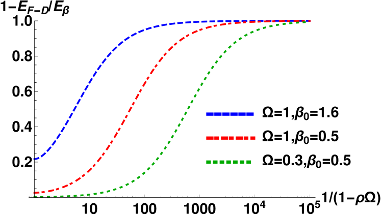
(a)

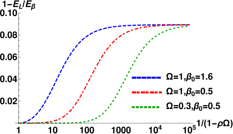
(b)

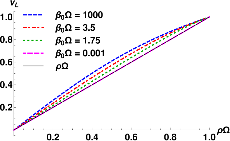
(c)

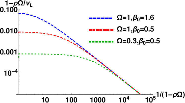
(d)

Figure 2: (a) Comparison between the energy density obtained from kinetic theory $E_{\rm F-D}$ (4) and the $\beta$-frame quantum energy density $E_{\beta}$ (16a); (b) Comparison between the energy densities $E_{L}$ (17) and $E_{\beta}$ (16a); (c) Comparison between the Landau velocity $v_{L}=\rho u^{\varphi}_{L}/u_{L}^{t}$ and the velocity $\rho\Omega$ correponding to rigid rotation; (d) Relative difference $1-\rho\Omega/v_{L}$ between $v_{L}$ and $\rho\Omega$ .

The Landau velocity $v_{L}=\rho u_{L}^{\varphi}/u_{L}^{0}\geq\rho\Omega$ is compared to $\rho\Omega$ in Fig. 2(c). The difference $1-\rho\Omega/v_{L}$ decreases to zero as the SOL is approached, while its value at the origin increases monotonically as $\beta_{0}\Omega$ is increased.

For completeness, we list below $\pi^{\mu\nu}_{L}$:

$$\pi^{\mu\nu}_{L}=\frac{2(E_{\beta}-E_{L})(3E_{L}-2E_{\beta})}{3(3E_{L}-E_{\beta})}u_{\beta}^{\mu}u_{\beta}^{\nu}+\frac{E_{\beta}-E_{L}}{3}g^{\mu\nu}\\ -\frac{E_{\beta}-E_{L}}{3E_{L}-E_{\beta}}(u_{\beta}^{\mu}W_{\beta}^{\nu}+u_{\beta}^{\nu}W_{\beta}^{\mu})-\frac{6E_{L}}{9E_{L}^{2}-E_{\beta}^{2}}W_{\beta}^{\mu}W_{\beta}^{\nu}.$$

6 Astrophysical application

Let us now apply our results in the context of the millisecond pulsar PSR J1748–2446ad reported in Ref. [18]. Its pulse frequency is $\nu\simeq 716\,{\rm Hz}$, such that the SOL is located at a distance $\rho_{\rm SOL}=c/2\pi\nu\simeq 66.685{\rm km}$ from the rotation axis. The typical surface temperature for a neutron star with characteristic age $\tau_{c}\geq 2.5\times 10^{7}\,{\rm years}$ is $T_{s}\simeq 10^{5}\,{\rm K}$ [19]. Its radius is $r_{s}\lesssim 16\,{\rm km}$ [18], such that the temperature on the rotation axis can be extrapolated as $T_{0}=T_{s}/\gamma_{s}\simeq 9.7\times 10^{4}\,{\rm K}$. Let us now investigate the magnitude of the quantum corrections for massless Dirac fermions dragged into rigid rotation by the pulsars magnetic field ($B_{\rm surf}\leq 1.1\times 10^{9}\,{\rm G}$ [18]) by considering the folowing quantity:

$$\delta E_{\rm QFT}=\frac{E_{\beta}}{E_{\rm F-D}}-1=\frac{10}{7\pi^{2}}\left(\frac{h\nu}{K_{B}T_{0}}\right)^{2}\left(\gamma^{2}-\frac{1}{4}\right)\\ \simeq 1.8\times 10^{-26}\left(\gamma^{2}-\frac{1}{4}\right),$$ (19)

where the appropriate units were reinserted. As pointed out in Ref. [17], the quantum correction is very small due to the presence of the Planck constant $h$. The value of $\gamma$ at which $E_{\beta}=2E_{\rm F-D}$ is $\gamma\simeq 7.4\times 10^{12}$, which would correspond for an electron to an energy of $m\gamma c^{2}\simeq 3.8\times 10^{18}\,{\rm eV}$, comparable to cosmic rays energies. At such high values of $\gamma$, the distance to the SOL is of order $\sim 6\times 10^{-22}\,{\rm m}$, where the rotation of the accretion disk is most likely no longer rigid.

Since our analysis was performed at the level of massless fermions, it is worth mentioning that in the case of the pulsar PSR J1748–2446ad, the relativistic coldness [8] has the value $\zeta_{0}=mc^{2}/k_{B}T_{0}\simeq 6.1\times 10^{4}$ in the case of electrons, while the ratio $mc^{2}/h\nu\simeq 1.7\times 10^{17}$ also has a large value. These numbers indicate that the massless limit results presented in this paper may be inaccurate close to the rotation axis, where the properties of RRTS are heavily influenced by the value of $m$ in both the kinetic theory [6] and in the QFT [14] approaches. Also in these latter references, it can be seen that the mass dependence dissapears in the vicinity of the SOL, such that at $\gamma\sim 7.4\times 10^{12}$, the particle constituents behave as though they were massless.

7 Conclusion

In summary, we investigated rigidly-rotating thermal states of massless Klein-Gordon and Dirac particles. In comparison to relativistic kinetic theory results, the QFT approach yields a non-ideal SET. An analysis of the quantum SET reveals the presence of quantum corrections to the energy density, as well as non-equilibrium terms such as the shear pressure tensor. These quantum terms become dominant as the speed of light surface (SOL) is approached. While for the Dirac field, the Landau frame can be defined everywhere up to the SOL, this is not so for the Klein-Gordon field, which we analysed based on the quantum corrections calculated in Ref. [17]. The Landau frame becomes everywhere well defined when the system is enclosed inside a boundary placed inside or on the SOL.

An evaluation of the order of magnitude of the quantum corrections in a realistic astrophysical system (i.e. for a millisecond pulsar) shows that for such systems, quantum corrections become important only at cosmic ray energies, in which case the rigid rotation must be mantained up to subnuclear distances from the SOL.

Appendix A QFT analysis of the Klein-Gordon field

It is well-known that the t.e.v. of the SET for the RRTS of the Klein-Gordon (KG) field is ill-defined throughout the whole space-time [14, 15]. It is also known that this anomalous behaviour is due to modes which are not present once the system is enclosed within a boundary which excludes the space outside of the SOL [15, 16, 23]. Moreover, the kinetic theory treatment of the same system allows the SET to be computed uneventfully everywhere inside the SOL. Recently, quantum corrections to these kinetic theory results were reported in Ref. [17]. The purpose of this appendix is to bridge the gap between the perturbative analysis of Ref. [17] and the expressions obtained from the exact QFT approach.

The QFT analysis of the RRTS of the KG field can be performed following Refs. [14, 15] by introducing co-rotating coordinates $x^{\mu}_{r}=(t_{r},\rho_{r},\varphi_{r},z_{r})$, defined via $\varphi_{r}=\varphi-\Omega t$, such that:

$$ds^{2}=-\gamma_{r}^{-2}dt_{r}^{2}+2\rho^{2}_{r}\Omega\,dt_{r}\,d\varphi_{r}+d\rho_{r}^{2}+\rho_{r}^{2}d\varphi_{r}^{2}+dz_{r}^{2}.$$ (20)

The KG field operator for scalar particles of mass $\mu$ can be expanded as:

$$\Phi(x_{r})=\sum_{m_{j}=-\infty}^{\infty}\int_{\mu}^{\infty}\omega_{j}\,d\omega_{j}\int_{-p_{j}}^{p_{j}}dk_{j}\left[f_{j}(x_{r})a_{j}+f^{*}_{j}(x_{r})a^{\dagger}_{j}\right],$$ (21)

where $f_{j}(x_{r})\equiv f_{\omega km}(x_{r})$ are the mode solutions of the KG equation [14, 15]:

$$f_{\omega km}(x_{r})=\frac{1}{\sqrt{8\pi^{2}|\omega|}}e^{-i\widetilde{\omega}t_{r}+im\varphi_{r}+ikz_{r}}J_{m}(q\rho_{r}).$$ (22)

In the above, $\widetilde{\omega}=\omega-\Omega m$ is the eigenvalue of the co-rotating Hamiltonian $H_{r}=i\partial_{t_{r}}$, while the transverse momentum $q$, longitudinal momentum $k$ and Minkowski energy $\omega$ satisfy $\omega=\sqrt{q^{2}+k^{2}+\mu^{2}}$, with $p=\sqrt{\omega^{2}-\mu^{2}}$ being the Minkowski momentum. The one-particle operators $a_{j}$ and $a_{j}^{\dagger}$ satisfy the canonical commutation relations $[a_{j},a_{j^{\prime}}^{\dagger}]=\delta(j,j^{\prime})$, where

$$\delta(j,j^{\prime})=\delta_{m_{j},m_{j^{\prime}}}\delta(k_{j}-k_{j^{\prime}})\frac{\delta(\omega_{j}-\omega_{j^{\prime}})}{|\omega_{j}|}.$$ (23)

Let us now consider the renormalised t.e.v. of the SET operator in the “new improved” [20] form corresponding to conformal coupling in Ref. [21]:

$$\braket{:T_{\mu\nu}:}_{\beta_{0}}=\\ \braket{:\frac{1}{3}\{\phi_{;\mu},\phi_{;\nu}\}-\frac{1}{6}\{\phi,\phi_{;\mu\nu}\}-\frac{1}{6}g_{\mu\nu}(\phi^{;\lambda}\phi_{;\lambda}+\mu^{2}\phi^{2}):}_{\beta_{0}},$$ (24)

where the colon indicates normal (Wick) ordering. The anticommutator $\{,\}$ was introduced to esure operator symmetrisation. The above t.e.v. can be computed starting from [14, 23]:

$$\braket{:a_{j}a^{\dagger}_{j^{\prime}}:}_{\beta_{0}}=\frac{\delta(j,j^{\prime})}{e^{\beta_{0}\widetilde{\omega}_{j}}-1}.$$ (25)

Introducing the notation $G_{abc}$ through [22]:

$$G_{abc}=\frac{1}{\pi^{2}}\sum_{m=-\infty}^{\infty}\int_{\mu}^{\infty}\frac{d\omega}{e^{\beta_{0}\widetilde{\omega}}-1}\int_{0}^{p}dk\,\omega^{a}q^{b}m^{c}J_{m}^{2}(q\rho),$$ (26)

the t.e.v. of $\phi^{2}$ and of the SET can be written as [22]:

$$\braket{:\phi^{2}:}_{\beta_{0}}= \frac{1}{2}G_{000},$$ (27)

$$\braket{:T_{tt}:}_{\beta_{0}}= \frac{1}{2}G_{200}+\frac{1}{24}\left(\frac{d^{2}}{d\rho^{2}}+\frac{1}{\rho}\frac{d}{d\rho}\right)G_{000},$$

$$\braket{:T_{\rho\rho}:}_{\beta_{0}}= \frac{1}{2}G_{020}-\frac{1}{2\rho^{2}}G_{002}+\frac{1}{8}\left(\frac{d^{2}}{d\rho^{2}}+\frac{5}{3\rho}\frac{d}{d\rho}\right)G_{000},$$

$$\braket{:T_{\varphi\varphi}:}_{\beta_{0}}= \frac{1}{2\rho^{2}}G_{002}-\frac{1}{24}\left(\rho^{2}\frac{d^{2}}{d\rho^{2}}+3\rho\frac{d}{d\rho}\right)G_{000},$$

$$\braket{:T_{zz}:}_{\beta_{0}}= \frac{1}{2}(G_{200}-G_{020}-\mu^{2}G_{000})-\frac{1}{24}\left(\frac{d^{2}}{d\rho^{2}}+\frac{1}{\rho}\frac{d}{d\rho}\right)G_{000},$$

$$\braket{:T_{t\varphi}:}_{\beta_{0}}= -\frac{1}{2}G_{101}.$$ (28)

The functions $G_{abc}$ (26) are clearly divergent due to the Bose-Einstein density of states factor $(e^{\beta_{0}\widetilde{\omega}}-1)^{-1}$. In this section, we will present a procedure to isolate the regular part $G_{abc}^{\rm reg}$ of $G_{abc}$ by splitting $G_{abc}$ as follows:

$$G_{abc}=G_{abc}^{\rm reg}+G_{abc}^{\infty},$$ (29)

where $G_{abc}^{\infty}$ absorbs the infinite part of $G_{abc}$. We will show that $G_{abc}^{\rm reg}$ leads to the corrections presented in Ref. [17].

The method that we will employ is analogous to that used in Ref. [14] for Dirac fermions, being based on expanding the Bose-Einstein density of states factor as follows [22]:

$$\frac{1}{e^{\beta_{0}(\omega-\Omega m)}-1}=\sum_{n=0}^{\infty}\frac{(-\Omega)^{n}}{n!}m^{n}\frac{d^{n}}{d\omega^{n}}\left(\frac{1}{e^{\beta_{0}\omega}-1}\right),$$ (30)

Since the left hand side of the above expression has a pole at $\omega=\Omega m$, the above expansion is not well defined when $\omega<\Omega m$. It is worth mentioning that the modes for which $\widetilde{\omega}<0$ are no longer allowed when the system is enclosed inside a boundary placed inside or on the SOL [15, 16]. Despite the fact that the modes with $\widetilde{\omega}<0$ cannot be excluded from the mode sum in Eq. (26), we will show that the above procedure can still be used to recover the results in Ref. [17].

Substituting the expansion (30) into Eq. (26) yields:

$$G_{abc}=\frac{1}{\pi^{2}}\sum_{n=0}^{\infty}\frac{(-\Omega)^{n}}{n!}\int_{\mu}^{\infty}d\omega\,\omega^{a}\frac{d^{n}}{d\omega^{n}}(e^{\beta_{0}\omega}-1)^{-1}\\ \times\int_{0}^{p}dk\,q^{b}\sum_{m=-\infty}^{\infty}m^{n+c}J_{m}^{2}(q\rho).$$ (31)

The sum over $m$ can be performed using the following formula:

$$\sum_{m=-\infty}^{\infty}m^{2n}J_{m}^{2}(z)=\sum_{j=0}^{n}\frac{\Gamma(j+\frac{1}{2})}{j!\sqrt{\pi}}a_{n,j}z^{2j},$$ (32)

where the coefficients $a_{n,j}$ can be determined as follows:

$$a_{n,j}=\frac{1}{(2j)!}\lim_{\alpha\rightarrow 0}\frac{d^{2n}}{d\alpha^{2n}}\left(2\sinh\frac{\alpha}{2}\right)^{2j},$$ (33)

such that $a_{n,j}$ vanishes when $j>n$. The following particular cases are required to evaluate Eqs. (27) and (28):

$$a_{j,j}=1,\qquad a_{j+1,j}=\frac{1}{12}j(2j+1)(2j+2),$$

$$a_{j+2,j}=\frac{1}{1440}j(2j+1)(2j+2)(2j+3)(2j+4)(5j-1).$$ (34)

Furthermore, the integral over $k$ in Eq. (31) can be performed using Eq. (A.11) in Ref. [14]:

$$\int_{0}^{p}dk\,q^{\nu}=\frac{\Gamma(\frac{\nu}{2}+1)\sqrt{\pi}}{2\Gamma(\frac{\nu+1}{2}+1)}p^{\nu+1}.$$ (35)

Let us apply the above procedure for $G_{000}$, which reduces to:

$$G_{000}=\frac{1}{\pi^{2}}\sum_{j=0}^{\infty}\frac{(\rho\Omega)^{2j}}{2j+1}\sum_{n=0}^{\infty}\frac{\Omega^{2n}a_{n+j,j}}{(2n+2j)!}\\ \times\int_{\mu}^{\infty}d\omega\,p^{2j+1}\frac{d^{2n+2j}}{d\omega^{2n+2j}}(e^{\beta_{0}\omega}-1)^{-1}.$$ (36)

In the massless case, $p=\omega$ and the integral over $\omega$ runs from $0$ to $\infty$. Noting that:

$$\int_{0}^{\infty}d\omega\,\omega^{2j+1}\frac{d^{2n+2j}}{d\omega^{2n+2j}}(e^{\beta_{0}\omega}-1)^{-1}=\\ (2j+1)!\times\begin{cases}{\displaystyle\frac{\pi^{2}}{6\beta_{0}^{2}}},&n=0,\\ {\displaystyle-\frac{1}{2}+\frac{1}{\beta_{0}}\lim_{\omega\rightarrow 0}\omega^{-1}},&n=1,\\ {\displaystyle\frac{1}{\beta_{0}}(2n-2)!\lim_{\omega\rightarrow 0}\omega^{-2n+1}},&n>1.\end{cases}$$ (37)

It can be seen that the case $n=0$ corresponds to $G_{000}^{\rm reg}$. The first term $-\frac{1}{2}$ in the $n=1$ piece represents a temperature-independent contribution (i.e. which survives in the limit of vanishing temperature, when $\beta_{0}\rightarrow\infty$). This is the analogue of the spurious contributions highlighted in Ref. [14], which are induced due to the construction of the thermal state with respect to the Minkowski (static) vacuum (see the Iyer vs. Vilenkin discussion in Ref. [14]). The second term in the $n=1$ piece and all further terms with $n>1$ are divergent, being induced by the infrared divergence of the Bose-Einstein density of states factor:

$$\frac{1}{e^{\beta_{0}\omega}-1}=\frac{1}{\beta_{0}\omega}-\frac{1}{2}+\text{odd, positive powers of }\beta_{0}\omega.$$ (38)

The result can be summarised as follows:

$$G_{000}^{\rm reg}= \frac{\gamma^{2}}{6\beta_{0}^{2}},$$

$$G_{000}^{\infty}= -\frac{\Omega^{2}\gamma^{2}}{24\pi^{2}}(\gamma^{2}-1)+\frac{\Omega^{2}}{\pi^{2}\beta_{0}}\sum_{j=0}^{\infty}(\rho\Omega)^{2j}$$

$$\times\sum_{n=0}^{\infty}\frac{\Omega^{2n}(2j)!(2n)!a_{n+j+1,j}}{(2n+2j+2)!}\lim_{\omega\rightarrow 0}\omega^{-2n-1}.$$ (39)

After a similar analysis of the rest of the terms appearing in Eq. (28), the following regular contributions $\phi^{2}_{\rm reg}$ and $T_{\mu\nu}^{\rm reg}$ to $\braket{:\phi^{2}:}_{\beta_{0}}$ and $\braket{:T_{\mu\nu}:}_{\beta_{0}}$ can be obtained:

$$\phi^{2}_{\rm reg}= \frac{\gamma^{2}}{6\beta_{0}^{2}},$$ (40)

$$T_{tt}^{\rm reg}= \frac{\pi^{2}\gamma^{4}}{90\beta_{0}^{4}}(4\gamma^{2}-1)+\frac{\Omega^{2}\gamma^{6}}{36\beta_{0}^{2}}(6\gamma^{2}-5),$$

$$T_{\rho\rho}^{\rm reg}= \frac{\pi^{2}\gamma^{4}}{90\beta_{0}^{4}}+\frac{\Omega^{2}\gamma^{6}}{36\beta_{0}^{2}},$$

$$\frac{1}{\rho^{2}}T_{\varphi\varphi}^{\rm reg}= \frac{\pi^{2}\gamma^{4}}{90\beta_{0}^{4}}(4\gamma^{2}-3)+\frac{\Omega^{2}\gamma^{6}}{36\beta_{0}^{2}}(6\gamma^{2}-5),$$

$$T_{zz}^{\rm reg}= \frac{\pi^{2}\gamma^{4}}{90\beta_{0}^{4}}-\frac{\Omega^{2}\gamma^{6}}{36\beta_{0}^{2}},$$

$$\frac{1}{\rho}T_{t\varphi}^{\rm reg}= -\rho\Omega\left[\frac{2\pi^{2}\gamma^{6}}{45\beta_{0}^{4}}+\frac{\Omega^{2}\gamma^{6}}{18\beta_{0}^{2}}(3\gamma^{2}-1)\right].$$ (41)

Performing the $\beta$-frame decomposition with respect to $u_{\beta}$ (2) on the above expressions yields Eqs. (12).

References

• [1] S. R. de Groot, W. A. van Leeuwen and Ch. G. van Weert, Relativistic kinetic theory - Principles and applications, North-Holland Publishing Company, Amsterdam, Netherlands, 1980.
• [2] C. Cercignani and G. M. Kremer, The relativistic Boltzmann equation: theory and applications, Birkhäuser Verlag, Basel, Switzerland, 2002.
• [3] F. Becattini, Phys. Rev. Lett. 108 (2012) 244502 .
• [4] F. Becattini, L. Bucciantini, E. Grossi, and L. Tinti, Eur. Phys. J. C 75 (2015) 191.
• [5] F. Becattini, Acta Physica Polonica B 47 (2016) 1819.
• [6] V. E. Ambru\cbs and R. Blaga, Annals of West University of Timisoara - Physics 58 (2015) 89.
• [7] V. E. Ambru\cbs and I. I. Cotăescu, Phys. Rev. D 94 (2016) 085022.
• [8] L. Rezzolla and O. Zanotti, Relativistic hydrodynamics, Oxford University Press, Oxford, UK, 2013.
• [9] D. L. Meier, Black hole astrophysics: The engine paradigm, Springer–Verlag, Berlin–Heidelberg, 2012.
• [10] I. Bouras, E. Molnár, H. Niemi, Z. Xu, A. El, O. Fochler, C. Greiner and D. H. Rischke, Phys. Rev. C 82 (2010) 024910.
• [11] C. Eckart, Phys. Rev. 58 (1940) 919.
• [12] L. D. Landau and E. M. Lifshitz, Fluid mechanics, 2nd ed., Pergamon Press, Oxford, UK, 1987.
• [13] P. Ván and T. S. Biró, AIP Conf. Proc. 1578 (2014) 114.
• [14] V. E. Ambru\cbs and E. Winstanley, Phys. Lett. B 734 (2014) 296.
• [15] G. Duffy and A. C. Ottewill, Phys. Rev. D 67 (2003) 044002.
• [16] N. Nicolaevici, Class. Quantum Grav. 18 (2001) 5407.
• [17] F. Becattini and E. Grossi, Phys. Rev. D 92 (2015) 045037.
• [18] J. W. T. Hessels, S. M. Ransom, I. H. Stairs, P. C. C. Freire, V. M. Kaspi, F. Camilo, Science 311​ (2006) 1901–1904.
• [19] N. K. Glendenning, Compact stars – Nuclear physics, particle physics, and general relativity, Springer-Verlag, New York, USA, 1997.
• [20] P. Candelas and D. Deutsch, Proc. R. Soc. Lond. A 354 (1977) 79–99.
• [21] N. D. Birrell and P. C. W. Davies, Quantum fields in curved space, Cambridge University Press, Oxford, 1982.
• [22] V. E. Ambru\cbs, PhD thesis (2014), eprint available at:
http://etheses.whiterose.ac.uk/id/eprint/7527.
• [23] A. Vilenkin, Phys. Rev. D 21, 2260 (1980).