Continuously heterogeneous hyper-objects in cryo-EM and 3-D movies of many temporal dimensions

Abstract

Single particle cryo-electron microscopy (EM) is an increasingly popular method for determining the 3-D structure of macromolecules from noisy 2-D images of single macromolecules whose orientations and positions are random and unknown. One of the great opportunities in cryo-EM is to recover the structure of macromolecules in heterogeneous samples, where multiple types or multiple conformations are mixed together. Indeed, in recent years, many tools have been introduced for the analysis of multiple discrete classes of molecules mixed together in a cryo-EM experiment. However, many interesting structures have a continuum of conformations which do not fit discrete models nicely; the analysis of such continuously heterogeneous models has remained a more elusive goal. In this manuscript we propose to represent heterogeneous molecules and similar structures as higher dimensional objects. We generalize the basic operations used in many existing reconstruction algorithms, making our approach generic in the sense that, in principle, existing algorithms can be adapted to reconstruct those higher dimensional objects. As proof of concept, we present a prototype of a new algorithm which we use to solve simulated reconstruction problems.

Keywords: hyper-molecules, hyper-objects, heterogeneity, continuous heterogeneity, cryo-EM, SPR, tomography, 4-D tomography, refinement, inverse problems, frequency marching

1 Introduction

Cryo-EM has been named Method of the Year 2015 by the journal Nature Methods due to the breakthroughs that the method facilitated in mapping the structure of molecules that are difficult to crystallize. Cryo-EM does not require crystallization necessary for X-ray crystallography, and unlike NMR it is not limited to small molecules. One of the additional great opportunities in cryo-EM, which has been noted, for example, in the surveys accompanying the Nature Methods announcement [1, 2, 3], is to overcome heterogeneity in the sample: in practice many samples contain two (or more) distinct types of molecules (or different conformations of the same molecule); methods like X-ray crystallography and NMR, which measure ensembles of particles, have a difficulty distinguishing between these different types. Many existing algorithms for the analysis of cryo-EM experimental data address the problem of recovering a finite number of distinct structures in heterogeneous samples. However, ”[large macromolecular assemblies] tend to be flexible, and although classification methods have come a long way when applied to biochemical mixtures or well-defined conformational states, the continuous motions seen for certain samples will challenge classification schemes and set a limit to achievable resolution, at least for a number of years.”[2] The purpose of this manuscript is to propose an approach to mapping continuously heterogeneous structures, and to demonstrate its applicability to cryo-EM.

The idea behind our approach is to generalize the tomography and cryo-EM problems of recovering a function over $\mathbb{R}^{3}$, representing a 3-D object, to the problem of recovering of a function over $\mathbb{R}^{3}\times\mathcal{T}$, where $\mathcal{T}$ captures the topology of the heterogeneity. We refer to these more general functions as hyper-volumes, hyper-objects or hyper-molecules. For example, loosely speaking, some types of continuous heterogeneity can be represented as functions over $\mathbb{R}^{4}$; tomography and cryo-EM can be generalized to the problem of recovering such 4-D objects. Indeed, the concept of 4-D tomography (4DCT) has been used in CT scans of patients, whose bodies change periodically with time as they breath (see, for example, [4]), but it is restricted to the case where both the orientation of each projection and its phase (time) in the breathing cycle are known. We discuss general topologies of heterogeneity, the case of unknown directions and “time,” and new approaches to the representation and regularization of the problem.

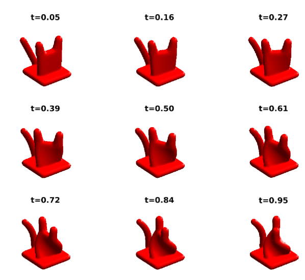
Figure 1: Samples of true object-instances from the simulated dataset at different values of the continuous parameter $t$, plotted at a level set

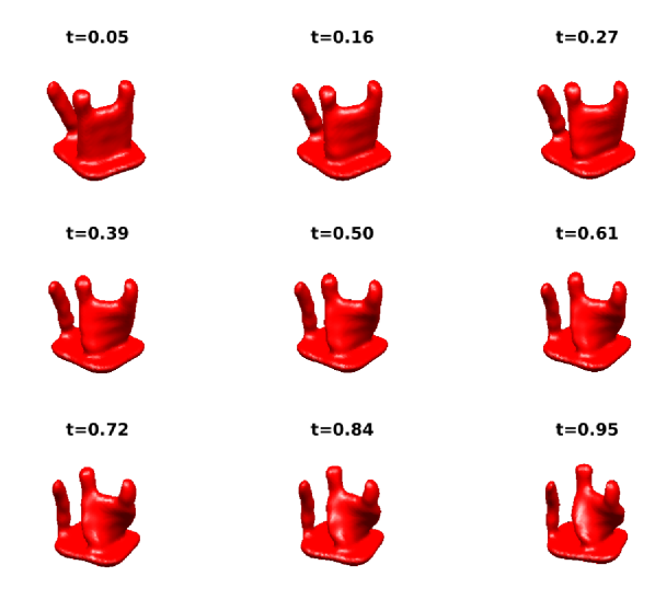
Figure 2: Samples of reconstructed object-instances at different values of the continuous $t$.

To illustrate the idea, we consider the heterogeneous object whose level sets are depicted in Figure 1. This object has a one dimensional heterogeneity variable in the range $t\in[0,1]$, so for each value of $t$ in this range, there is a 3-D object that is different from the 3-D object at a different value of $t$. However, the objects are continuous, in the sense that the object at $t$ is very similar to the object at $t^{\prime}$ if the difference $|t-t^{\prime}|$ is small. This idea is somewhat similar to a short 2-D video where the frame at each moment is generally relatively similar to adjacent frames. In movies, this similarity allows us, for example, to compress the video, because the video can be represented using much less information than a collection of independent frames.

Going back to our heterogeneous object, suppose that we have a 3-D movie of this object as we change the value of the parameter $t$ in time (examples available at http://roy.lederman.name/cryo-em), and suppose that we focus on a single “voxel” or coordinate in 3-D space as time passes and measure the mass at this point at every moment. Suppose that at $t=0$ none of the mass of the object is positioned at our point in space, but as time passes, one of the “ears” passes through our point and than exits before $t=1$. Then, we would see a curve, to which we could fit some polynomial; we could fit this polynomial even if we had only sample points in time, and we could use it to interpolate the value of our voxel at times when we did not sample the voxel. The mass at our voxel can be represented using the expansion

$$\mathcal{V}(t)=\sum_{q}a_{q}P_{q}(t).$$ (1)

Looking at all the voxels in our 3-D movie, we can fit such curves to each voxel, and obtain a representation of our object (discretized in space); for every sample point $(x_{1},x_{2},x_{3})$ in space, we have the polynomials with the coefficients $a_{q}(x_{1},x_{2},x_{3})$ of that particular point:

$$\mathcal{V}(x_{1},x_{2},x_{3},t)=\sum_{q}a_{q}(x_{1},x_{2},x_{3})P_{q}(t).$$ (2)

A very high degree polynomial would allow us to capture a very high frequency function, but the expansion is typically truncated (or the high frequency are weighted down) to reflect smoothness in the model and also due to the limited number of samples that are available, and for practical computational reasons. Now consider how a 3-D object is typically represented when there is no heterogeneity; typically the representation is equivalent to some linear combination of coefficients so that

$$\mathcal{V}(x_{1},x_{2},x_{3})=\sum_{k}h_{k}\phi_{k}(x_{1},x_{2},x_{3}),$$ (3)

with $\phi_{k}(x_{1},x_{2},x_{3})$ some spatial basis functions. In cryo-EM, the objects are often represented as samples at grid-points in the Fourier domain, so that the index $k$ encapsulates the three indices of points in the Fourier domain. The expansion is truncated to a finite number of frequency samples, and often some frequencies are penalized so that they would have lower amplitude; this reflects a preference to smoother objects. Combining our discussion of the object and its variability over “time” we obtain a generalization of a 3-D object to a “3-D movie,” or hyper-object:

$$\mathcal{V}(x_{1},x_{2},x_{3},t)=\sum_{k,q}a_{k,q}\phi_{k}(x_{1},x_{2},x_{3})P_{q}(t).$$ (4)

One of the main difficulties in cryo-EM is that the 2-D images of the object are given without information about the directing from which each image was taken, and the challenge is to reconstruct the 3-D object from these images without knowledge of these direction; various algorithms have been constructed for this difficult task. In the case of heterogeneous objects, the challenge is to reconstruct hyper-objects from images in the absence of both the direction of each image and the value $t$ that reflects the “time in the 3-D movie” or the version of the object which has recorded in that image. Various algorithms have been constructed for the case of discrete heterogeneity, where there are several distinct objects (a collection of independent “3-D still scenes” as opposed to a continuous “3-D movie”). Continuously heterogeneous objects, such as the object in Figure 1, are often treated as if they were distinct independent objects; this does not capture the continuous nature of the model and does not take advantage of this property to improve the reconstruction. Very loosely speaking, this would be analogous to averaging a movie in 1 second windows, then presenting these one-second averaged windows in random order.

We submit that 1) capturing the continuous nature of hyper-objects contributes to the reconstruction and understanding of the objects, 2) the problem of reconstructing without knowing the direction and $t$ is analogous to the problem of reconstructing without knowing the directions (we discuss some of the differences that do indeed arise), and 3) our general approach can be applied in a wide range of reconstruction algorithms, based on this analogy. Indeed, the reconstruction of distinct objects (discrete heterogeneity) can be viewed as a special case of our approach.

We propose several directions for implementing the idea of using continuity or approximate continuity, and discuss in more detail one such approach based on Equation (4). We argue that different variations are useful for different models (for example, spacial bases for local variability in a larger object). Furthermore, we argue that the approach can be applied to rather arbitrary topologies of heterogeneity: the line segment in our example, the cyclic pattern in 4DCT, two dimensional surfaces etc. We demonstrate our approach in a basic prototype as proof-of-concept, but emphasize that these ideas can be implemented in any of the many approaches applied to problems like cryo-EM. The results of the reconstruction using our prototype are demonstrated in Figure 2.

This manuscript is organized as follows. In Section 2, we summarize some standard results used in this manuscript. In Section 3, we briefly review a simplified model of cryo-EM and reformulate some of the tools used in cryo-EM algorithms in a way that we find useful for generalization. In Section 4, we discuss the generalization of tomography and cryo-EM to heterogeneous objects. In Section 5, we present a crude algorithm which we implemented to investigate one version of the ideas presented in this manuscript. For the sake of completeness we briefly review some of the new ideas used in this implementation, but argue that this is certainly not the only way to implement the idea of hyper-object reconstruction. Our preliminary results are presented in Section 6. A Brief summary and discussion of future work is presented in Section 7. Brief conclusions are presented in Section 8.

Additional examples and video visualization of the results are available at http://roy.lederman.name/cryo-em.

Remark 1 (Terminology: “representation”).

Our use of the term “representation” in the context of this manuscript is very different from the context in which we use the term in [5]. However, we have not found a better term that would avoid this confusion. In this manuscript “representation” is a way of expressing a function or a problem, typically an expansion of a function in some basis, whereas in [5] it is a technical representation theory term. These two works are independent and largely unrelated on a technical level; the conceptual relation between the two is the motivation to treat heterogeneity as “just another variable.”

2 Preliminaries

Table 1: Table of Notation

$\mathcal{F}_{Q}\mathcal{V}$	the Fourier transform of the function $\mathcal{V}$ in the variable $Q$
$\hat{\mathcal{M}}$	the Fourier transform of $V$ in spacial coordinates
$R{\mathbf{x}}$	the vector $\mathbf{x}$ rotated by $R$
$R\circ\mathcal{V}$	the function $\mathcal{V}$ rotated by $R$, so that $\left(R\circ\mathcal{V}\right)(\mathbf{x})=\mathcal{V}(R^{-1}\mathbf{x})$

2.1 Spherical harmonics and rotations

In this subsection we summarize some of the properties of spherical harmonics.

The normalized spherical harmonic, denoted by $Y_{l}^{m}(\theta,\phi)$, with integer $l\geq 0$ and $-l\leq m\leq l$, is defined by the formula:

$$Y_{l}^{m}(\theta,\varphi)=\sqrt{\frac{2l+1}{4\pi}\frac{(l-m)!}{(l+m)!}}P_{l}^{m}\left(\cos(\theta)\right)\exp(im\varphi),$$ (5)

where $P_{l}^{m}$ are the associated Legendre polynomials (see, for example [6]). The spherical harmonics are an orthonormal basis of $\mathcal{L}^{2}(S^{2})$, so that

$$\int Y_{l}^{m}(\theta,\varphi){\left(Y_{l^{\prime}}^{m^{\prime}}(\theta,\varphi)\right)}^{*}\sin(\theta)d\theta d\varphi=\delta_{ll^{\prime}}\delta_{mm^{\prime}},$$ (6)

and the expansion of any function $f\in\mathcal{L}^{2}(S^{2})$ on the sphere in this basis is

$$f(\theta,\varphi)=\sum_{l=0}^{\infty}\sum_{m=-l}^{l}v_{lm}Y_{l}^{m}(\theta,\varphi),$$ (7)

with the appropriate expansion coefficients $v_{lm}$.

Any arbitrary rotation of a 2-D sphere can be represented by three Euler angles, we denote the rotation operator by $R(\alpha,\beta,\gamma)$. The expansion of a rotated function $R(\alpha,\beta,\gamma)\circ f$ is given by the formula

$$\left(R(\alpha,\beta,\gamma)\circ f\right)(\theta,\varphi)=\sum_{l=0}^{\infty}\sum_{m=-l}^{l}\tilde{v}_{lm}Y_{l}^{m}(\theta,\varphi).$$ (8)

where the coefficients in the expansion are

$$\tilde{v}_{lm}=\sum_{m^{\prime}=-l}^{l}\rho^{(l)}_{mm^{\prime}}(\alpha,\beta,\gamma)v_{lm^{\prime}},$$ (9)

with $\rho^{(l)}(\alpha,\beta,\gamma)$ the $l$-th order of the appropriate form of the Wigner-D matrix for the rotation (see, for example [7]).

The restriction $f(\varphi)$ of a function $f(\theta,\varphi)$ on a sphere to the “equator” is given by

$$f(\varphi)=f(\pi/2,\varphi).$$ (10)

It immediately follows that the Fourier expansion of the restricted function is

$$f(\varphi)=\sum_{l=0}^{\infty}\sum_{m=-l}^{l}v_{lm}Y_{l}^{m}(\pi/2,0)\exp(im\varphi)=\sum_{m=-\infty}^{\infty}h_{m}\exp(im\varphi).$$ (11)

where

$$h_{m}=\sum_{l=|m|}^{\infty}v_{lm}Y_{l}^{m}(\pi/2,0).$$ (12)

2.2 Haar basis

The Haar wavelet mother function is defined by the formula

$$\varphi(t)=\begin{cases}1&\text{for~{}}0\leq t\leq 1/2\\ -1&\text{for~{}}1/2<t\leq 1\\ 0&otherwise.\end{cases}$$ (13)

The Haar function $\psi_{n,k}(t)$ is defined by the formula

$$\psi_{n,k}(t)=2^{n/2}\varphi(2^{n}t-k),$$ (14)

for all integer $n,k$. For the purpose of our discussion of a finite intervals, it is convenient to take $n\geq 0$ and $0\leq k\leq 2^{n}-1$ and add the constant function. Higher dimensional Haar basis functions are composed as the tensor product of one dimensional Haar functions.

A truncated expansion of a function in the Haar basis is simply a piece-wise constant function. In other words, the space is divided into $2^{K}$ intervals, and the function is constant in each of these intervals. However, the Haar basis can also be thought of as a multiscale/tree decomposition of an interval (or hypercube), into sub-intervals. The multiscale tree structure of the functions is useful in analysis.

3 Setup and reformulation

3.1 The representation of objects

An object or a “volume” $\mathcal{V}$ is a function over $\mathcal{X}$ (in our case, $\mathcal{X}=\mathbb{R}^{3}$ is coordinates in space). The Fourier transform of the object, which we denote by $\mathcal{F}_{X}\mathcal{V}=\hat{\mathcal{V}}$, is a function over $\Omega$ (in our case $\Omega=\mathbb{R}^{3}$ are coordinates in the Fourier domain). For the purpose of this discussion, we assume that the objects are continuous with respect to $X$ and $\Omega$ (this assumption can be relaxed).

In applications, the function $\mathcal{V}$ must be discretized in some way, if only so that we can represent it in a digital computer. Furthermore, the choice of discretization reflects (implicitly or explicitly) priors or regularization of the object, which are required in order to make the tomography problem tractable.

The object $\mathcal{V}$ is often represented using discrete samples of $\mathbb{R}^{3}$ on a regular grid, restricted to some finite box which is sufficiently large to contain the molecule which we wish to reconstruct (e.g., a $128\times 128\times 128$ grid); points off the grid are sometimes evaluated using some continuous interpolation from the grid points (although non-continuous voxels are also considered). Since many of operations in cryo-EM are naturally represented in the Fourier domain, and as it is often assumed that $\mathcal{V}$ (or some low-resolution version of it) is band-limited, many cryo-EM algorithms and programs use a similar regular grid in the Fourier domain to represent samples of $\hat{\mathcal{V}}$ in $\Omega$. In works such as [8], the Fourier transform $\hat{\mathcal{V}}$ of the object is represented as concentric shells sampled at various radii.

These different representations assume certain properties of $\mathcal{V}$; the regular grid in a box in the real space assumes that the $\mathcal{V}$ is compactly supported in real space (the choice of interpolation scheme implies additional smoothness assumptions). The regular grid in the Fourier domain implies, for example, that the function is band-limited. The representation in concentric shells in the Fourier domain makes similar assumptions on the band-limit of the function and is computationally convenient; each concentric shell can be represented using spherical harmonics rather than samples on the sphere, yielding a natural continuous representation that has no directional bias (unlike the regular grid).

Loosely speaking, different common representations of an object can be summarized as vectors of coefficients. For example, a vector composed of all the values sampled at the grid points of a 3-D Fourier transform of an object. In standard linear representations of objects, the object (or its Fourier transform) is written as

$$\mathcal{V}(x_{1},x_{2},x_{3})=\sum_{i}w_{i}\varphi_{i}(x_{1},x_{2},x_{3}),$$ (15)

or

$$\hat{\mathcal{V}}(\omega_{1},\omega_{2},\omega_{3})=\sum_{i}w_{i}\hat{\varphi}_{i}(\omega_{1},\omega_{2},\omega_{3}),$$ (16)

where $\mathbf{w}$ is the vector of coefficients, $w_{i}$ the $i$-th element of the vector, $\varphi_{i}$ some basis functions appropriate for that representation, and $\hat{\varphi}_{i}$ their Fourier transforms.

Typically, the representation of objects is continuous, in the sense that small rotations and translations of the object, and small changes in the object, result in small changes to the coefficients in the representation. This property is not necessarily uniform: for example, some types of perturbation in the objects can have a larger effect on high frequency components than on low frequency components of some representations.

The choice of basis and the truncation of the basis to a finite number of basis functions (e.g., finite cube in space and finite resolution) restricts the functions that can be represented to certain function spaces. This serves as an implicit regularization in algorithms for the reconstruction of molecules (see below), and it is sometimes augmented by more explicit regularization or priors on the object.

Bases that are better suited to a problem allow high accuracy approximation of the relevant functions using fewer coefficients, or more efficient computation. Loosely speaking, a function that is efficiently approximated in one basis can be approximated in other reasonable bases even if the representation is less efficient and requires more basis functions. For example, a low order polynomial can be represented efficiently as a linear combination of polynomials basis functions, and it can also be approximated well by equally spaced samples with linear interpolation between the sample points. In this sense, all the bases are “equivalent.” However, an efficient basis is also an implicit regularizer which restricts the space of functions. For example, low order polynomials are smooth and have restricted oscillations, whereas the sampling scheme above has more degrees of freedom and represents functions that are not smooth and functions that oscillate more. Such restriction can be introduced in any arbitrary representation explicitly as constraints, filters, penalties or regularizers.

3.2 Cryo-EM

Electron Microscopy is an important tool for recovering the 3-D structure of molecules. Of particular interest in the context of this manuscript is Single Particle Reconstruction (SPR), and more specifically, cryo-EM, where multiple noisy 2-D projections, ideally of identical particles in different orientations, are used in order to recover the 3-D structure. The following formula is a simplified noiseless imaging model of SPR, for obtaining the noiseless image $I^{(i)}$ from a object $\mathcal{V}$ (representing the molecule’s density):

$$I^{(i)}(x_{1},x_{2})=\left(\mathcal{P}R_{i}\mathcal{V}\right)(x_{1},x_{2})=\int_{\mathbb{R}}\mathcal{V}(R_{i}^{-1}{\mathbf{x}})dx_{3},$$ (17)

where ${\mathbf{x}}=(x_{1},x_{2},x_{3})^{\intercal}$ and $R_{i}$ is the rotation that determines the orientation of the molecule. In other words, the model is that the molecule is rotated in a random direction, and the recorded image is the top-view projection of the rotated molecule, integrating out the $x_{3}$ or $z$ axis. In the Fourier domain, the Fourier transform $\hat{I}^{(i)}$ of an image is a slice of the Fourier transform $\hat{\mathcal{V}}$ through the origin:

$$\hat{I}^{(i)}(\omega_{1},\omega_{2})=\hat{\mathcal{V}}(R_{i}^{-1}{\mathbf{\omega}})$$ (18)

where ${\mathbf{\omega}}=(\omega_{1},\omega_{2},0)^{\intercal}$ and $R_{i}$ is the random rotation.

One of the characteristic properties of cryo-EM SPR that sets it apart from other tomography techniques is that the orientation $R_{i}$ of the molecule in each image is unknown in cryo-EM, whereas in other tomography techniques the rotation angles are typically recorded with the measurements.

The analysis of cryo-EM images is further complicated by many additional effects, some of the most notable are:

• extremely high levels of noise, far exceeding the signal in magnitude (see sample images in Figure 3),

• filters associated with the imaging process (CTF),

• an unknown shift of each image in the image plane,

• and the discretization of the measurements.

More detailed discussions of these challenges, and various other challenges can be found, for example, in [9]. Since these aspects are studied extensively in other works, and since the goal of this work is to introduce a new generalization of previous works, we will not discuss these aspects in much detail when they do not raise too many new issues that are of particular interest in continuous heterogeneity at the level of this preliminary discussion. We note that in our experiments we use simulated data with high levels of noise.

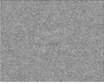
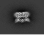
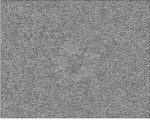
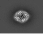
Figure 3: Left: two raw experimental images of TRPV1, available via EMDB 5778 [10]. Right: computed projections of TRPV1 which are the closest to the images on their left.

3.3 The tomography problem in cryo-EM

Suppose that we are given a set of images $\{I^{(i)}\}_{i=1}^{n}$ with the orientation $\{R_{i}\}_{i=1}^{n}$ of each image. Then, the reconstruction problem in cryo-EM is a classic tomography problem. In the Fourier domain, the model in equation (18) suggests that the problem is to reconstruct $\hat{\mathcal{V}}$ from (very noisy) slices of the Fourier transform of the object. This problem is ill-posed even in the noiseless case since we have no information about the values of $\hat{\mathcal{V}}$ at points between the slices. However, additional priors and assumptions on the properties of the object make the problem more tractable.

For the purpose of our discussion of tomography, we propose a further simplified description of the tomography problem, a one frequency pixel model of tomography, where we receive scalar samples $S_{i}$ of $\hat{\mathcal{V}}$, each at a given frequency point $\omega^{i}=(\omega^{i}_{1},\omega^{i}_{2},\omega^{i}_{3})^{\intercal}$:

$$S^{i}=\hat{\mathcal{V}}(\omega^{i}_{1},\omega^{i}_{2},\omega^{i}_{3}).$$ (19)

It is easy to see that if the Fourier transform of each image $\hat{I}^{(i)}$ in (18) is considered to be a (finite) collection of samples of $\hat{\mathcal{V}}$ at various frequency points, then the one frequency pixel model (19) describes the same model as (18), with the latter grouping together samples into images.

Taking into account the discussion of representing an object as a vector $\mathbf{w}$ of coefficients of some arbitrary linear expansion (15), we propose a more general linear operator formulation of linear models such as (17), (18) or (19), which simply states that each (noiseless) measurement is some vector of coefficients $\mathbf{y^{(i)}}$ given by a linear operation of the vector of coefficients $\mathbf{w}$:

$$\mathbf{y^{(i)}}=A^{(i)}\mathbf{w}.$$ (20)

In the cryo-EM imaging model, the linear operator $A^{(i)}$ captures the operation of rotating a molecule, projecting it and representing the resulting noiseless image using the vector of coefficients $\mathbf{y^{(i)}}$ (more comprehensive practical models also take into account the CTF, shifts, discretization, noise, etc.).

3.4 Unknown orientations, and reconstruction algorithms in cryo-EM SPR

One of the characteristics of the cryo-EM SPR problem that sets it apart from other tomography problems, is that the orientations $R_{i}$ of each image is unknown, making the problem severely ill-posed.

For the purpose of this discussion, we make a simplistic distinction between two approaches to the cryo-EM reconstruction problem: object-free image alignment, and direct object estimation. The object-free image alignment approach typically takes advantage of the projection-slice theorem to estimate the rotation $R_{i}$ of each image with respect to others based on the intersection of slices in the Fourier domain (see, for example, [11, 12, 13, 14]). Once the rotations are recovered, the next step is the tomography problem of estimating the object given the rotations. In the current manuscript, we focus on methods of direct object estimation, often called refinement, which alternate between refining an estimate of the object, and estimating the rotation of each image with respect to the object: given an estimated object $\mathcal{V}^{(n)}$ at step $n$, estimate the most likely orientation $R_{n,i}$ of the image recorded in the $i$-th image, for all images:

$$R_{(n,i)}=\operatorname*{arg\,min}_{R}\|A(R)\mathcal{V}^{(n)}-I^{(i)}\|,$$ (21)

where $A(R)$ is the operator which produces an image from the object $\mathcal{V}^{(n)}$, rotated to orientation $R$, and $I^{(i)}$ is the $i$-th recorded image. In practice, this minimization is typically performed by comparing each image to a set of computed template projections of the estimated object at some sampled values of $R$. Given these estimated rotations, produce a new estimate of the object, for example by solving:

$$\mathcal{V}^{(n+1)}=\operatorname*{arg\,min}_{\mathcal{V}}\sum_{i=1}^{N}\|A(R_{(n,i)})\mathcal{V}-I^{(i)}\|^{2},$$ (22)

possibly with some additional regularization terms. Some popular refinement software packages and algorithms follow more elaborate statistical approaches (e.g., [15, 16, 17, 18, 19, 20]) such as the Bayesian approach, and other optimization schemes (e.g., stochastic gradient descent in [21]). Since these approaches use similar fundamental operators and due to the limited scope of this manuscript, we will restrict our attention to conventional refinement algorithms and argue that our approach generalizes such algorithms to hyper-molecules. Our approach can be used in a similar way to generalize more elaborate algorithms.

3.5 Frequency marching

Several refinement tools such as RELION[18, 19] and FREALIGN [17, 22, 23] gradually increase the resolution of the estimated object as they iterate. In [8], this concept is reformulated as frequency marching: starting the iterative process with a representation of the object that uses only a small number of low frequency basis functions, and adding higher frequency basis functions to the expansion at subsequent refinement iterations.

Frequency marching highlights the fact that use of basis functions is not merely an technical implementation detail of how to store a function digitally, but rather a key tool at the heart of the algorithm.

3.6 Heterogeneity

So far, we have assumed that all the molecules being imaged in an experiment are identical copies of each other, so that all the images are projections of identical copies of the object $\mathcal{V}$, from different directions. However, in practice, the molecules in a given sample may differ from one another for various reasons. For example, the sample may contain several types of different molecules due to some contamination or feature of the experiment. Alternatively, the molecules which are studied may have several different conformations or states, or some local variability. The heterogeneity may be discrete (e.g., in the case of distinct different molecules), continuous (in the case of molecules with continuous variability), or a mixture of continuous elements and discrete elements.

In the heterogeneous settings, the simplified noiseless imaging model of the homogeneous case (see (17)) is generalized to

$$I^{(i)}(x_{1},x_{2})=\left(\mathcal{P}R_{i}\mathcal{V}[t_{i}]\right)(x_{1},x_{2})=\int_{\mathbb{R}}\mathcal{V}[t_{i}](R_{i}^{-1}{\mathbf{x}})dx_{3},$$ (23)

where $\mathcal{V}[t_{i}]$ is the objects imaged in sample $i$. The generalized operator formulation (20) is

$$y^{(i)}=A^{(i)}\mathbf{w}^{(t_{i})},$$ (24)

where $\mathbf{w}^{(t_{i})}$ is the vector of coefficients in the representation of the object $\mathcal{V}[t_{i}]$.

Most existing algorithms and software tools treat only the case of discrete heterogeneity. In conventional refinement algorithms, discrete classes of molecules are reconstructed by modeling multiple independent objects (see, for example [24]); given multiple estimated objects $\{\mathcal{V}^{(n)}[l]\}_{l=1}^{L}$, we estimate the most likely pair of class $l_{(n,i)}$ and orientation $R_{(n,i)}$ for each images, and proceed to produce a new estimate of each objects based on the the images assigned to it. For example, the generalization of (21) and (22) is

$$(R_{(n,i)},l_{(n,i)})=\operatorname*{arg\,min}_{(R,l)}\|A(R)\mathcal{V}^{(n)}[l]-I^{(i)}\|,$$ (25)

and

$$\mathcal{V}^{(n+1)}[l]=\operatorname*{arg\,min}_{\mathcal{V}}\sum_{i:l_{i}=l}\|A(R_{(n,i)})\mathcal{V}-I^{(i)}\|^{2},$$ (26)

A similar generalization is used in more elaborate algorithms (e.g., [15, 18]) and in software packages such as RELION[19]. Other approaches to heterogeneity require some method of recovering the rotation of the images although the images reflect mixtures of projections of different molecules (e.g., [25, 26]). We treat heterogeneity in object-free algorithms in [5] (with generalization to continuous heterogeneity - in preparation). Another recent independent work on object-free reconstruction [27] proposes to iterate between estimating the orientations and estimating the class labels based on pairwise relations between images. A different perspective on object-free algorithms for continuous heterogeneity, proposed in [28, 29], is to construct a manifold of images and study the low dimensional structures induced by rotations and heterogeneity.

Currently, the prevailing approach to continuous heterogeneity is to treat the object roughly as if it were a collection of discrete independent objects, rather than a continuum of objects. In this manuscript manuscript we investigate whether we can capture the continuous nature of the states, and even take advantage of it in reconstruction.

4 Analytical apparatus

4.1 Heterogeneous molecules - “hyper-molecules”

The purpose of this section is to generalize the definition of an object to a hyper-object, which represents a heterogeneous set of objects, simply by adding a variable that identifies each object instance.

To generalize the definition of an object to an hyper-object, we define a family of objects $\mathcal{M}$ as a function over $\mathcal{X}\times\mathcal{T}$, where $\mathcal{T}$ is the index set or parameterization of the family of objects. The evaluation of the density of an object at the coordinates $(x_{1},x_{2},x_{3})$, is analogous to the evaluation of a hyper-object at the coordinates $((x_{1},x_{2},x_{3}),t)$, which means choosing the object instance with the index $t$ and evaluating the density of that object at the coordinates $(x_{1},x_{2},x_{3})$. To illustrate the notation in the discrete case, suppose that we have only two distinct objects, then $\mathcal{T}=\{0,1\}$, and the object instances evaluated at $(x_{1},x_{2},x_{3})\in\mathcal{X}$ are $\mathcal{M}((x_{1},x_{2},x_{3}),0)$ and $\mathcal{M}((x_{1},x_{2},x_{3}),1)$. In the continuous case, suppose that we parameterize the hyper-objects by $\mathcal{T}=[0,1]$, then the object at $t\in\mathcal{T}$ evaluated at $(x_{1},x_{2},x_{3})$ is $\mathcal{M}((x_{1},x_{2},x_{3}),t)$. We note that, in general, $\mathcal{T}$ can have various topologies (discrete, an interval, a subset of a multi dimensional space, a torus, combinations thereof, etc.). For example, in 4DCT, the topology of heterogeneity may capture the cyclic behavior of breathing (as opposed to an interval with independent ends); in cryo-EM it may capture a one dimensional variability in states, or, for example, independent local variability in two different areas of the molecule.

We denote by $\mathcal{F}_{X}$ the Fourier transform which integrate over the coordinate space $\mathcal{X}$, and does not interact with the parameterization $\mathcal{T}$, so the Fourier transform of the object indexed by $t\in\mathcal{T}$, and evaluate at the frequency $(\omega_{1},\omega_{2},\omega_{3})$ is $\hat{\mathcal{M}}((\omega_{1},\omega_{2},\omega_{3}),t)=\left(\mathcal{F}_{X}\mathcal{M}\right)((\omega_{1},\omega_{2},\omega_{3}),t)$.

Finally, we define a transform $\mathcal{L}_{T}$ on the parameterization $\mathcal{T}$ which is analogous to $\mathcal{F}_{X}$. For example, suppose that $\mathcal{T}=\{0,1,\ldots,M-1\}$, and suppose that $\mathcal{L}_{T}$ is the discrete Fourier transform. Then, we have the “parameter-wise” discrete Fourier transform of the object evaluated at parameter frequency $\tau$ and coordinates $(x_{1},x_{2},x_{3})$, $\left(\mathcal{L}_{T}\mathcal{M}\right)((x_{1},x_{2},x_{3}),\tau)$. In this case, $\tau=0$ yields the average of all objects: $\left(\mathcal{L}_{T}\mathcal{M}\right)((x_{1},x_{2},x_{3}),0)\propto\frac{1}{M}\sum_{t=0}^{M-1}\mathcal{M}((x_{1},x_{2},x_{3}),t)$. We may also apply both transforms: $\left(\mathcal{L}_{T}\mathcal{F}_{X}\mathcal{M}\right)((\omega_{1},\omega_{2},\omega_{3}),\tau)$. For the purpose of this discussion, we assume that the operators commute:
$\left(\mathcal{L}_{T}\mathcal{F}_{X}\mathcal{M}\right)((\omega_{1},\omega_{2},\omega_{3}),\tau)=\left(\mathcal{F}_{X}\mathcal{L}_{T}\mathcal{M}\right)((\omega_{1},\omega_{2},\omega_{3}),\tau)$.

4.2 Tomography of hyper-objects

The caricature one frequency pixel model of tomography (19) describes tomography as the inverse problem of recovering the Fourier transform of a object $\mathcal{V}$ from many noisy samples $\{I^{i}\}_{i=1}^{n}$ at known frequency coordinates $\{(\omega^{i}_{1},\omega^{i}_{2},\omega^{i}_{3})\}_{i=1}^{n}$ (with some constraints or regularization to make the inverse problem tractable).

This description of the tomography problem generalizes naturally to hyper-objects: the one frequency pixel model of hyper-object tomography is the inverse problem of recovering $\mathcal{F}_{X}\mathcal{M}$ from many noisy samples $\{I^{i}\}_{i=1}^{n}$ at known frequencies and values of the heterogeneity index $\{((\omega^{i}_{1},\omega^{i}_{2},\omega^{i}_{3}),t_{i})\}_{i=1}^{n}$, with some analogous constraints or regularization of the hyper-object. In the discrete case, this simply means that for each sample, we have the label $t_{i}$ of the the object which was measured, and the frequency coordinates of the sample $(\omega^{i}_{1},\omega^{i}_{2},\omega^{i}_{3})$, and we may collect all the samples of each object and proceed to process each object independently from the others.

In computed tomography (CT), 4-D tomography technology[4] (4DCT) has been proposed in order to image the body of a patient in different states of the breathing cycle, so that $\mathcal{T}$ is time or phase within a breathing cycle. In 4DCT, as in classic CT, the orientation of each image is known; in addition, the position of each image in the breathing cycle is recorded using external means. The original 4DCT reconstruction algorithms binned the images according to their position in the cycle and then reconstructed an independent objects from each discrete bin. In recent years, regularization techniques have been introduced in order to take advantage of the relation between the volumes in different phases of the cycle (see, for example, [30, 31, 32, 33]).

4.3 The representation of heterogeneous objects - the discrete case

When there are K classes of objects, they can be represented as K vectors of coefficients. Suppose that $\mathbf{w}^{(k)}$ is the vector of coefficients associated with the representation of the $k$-th object, with ${w}^{(k)}_{i}$ the $i$-th element of this vector. Obviously, we can rewrite these as columns of a matrix $W$, such that $W_{ik}={w}^{(k)}_{i}$, and the $k$-th object as

$$\hat{\mathcal{M}}((\omega_{1},\omega_{2},\omega_{3}),k)=\sum_{i}W_{ik}\varphi_{i}(\omega_{1},\omega_{2},\omega_{3}).$$ (27)

Clearly, ${\mathcal{M}}((x_{1},x_{2},x_{3}),k)$ is equivalent to $\mathcal{V}[k](x_{1},x_{2},x_{3})$ used in (23), so that in the discrete case this formulation of the problem is equivalent to the classic formulation used in existing cryo-EM algorithms which store multiple independent models of objects.

As a step toward the discussion below of representations of continuously heterogeneous objects, we present some non-formal motivation through the following trivial accounting exercise. Suppose that $U$ is a $K\times K$ unitary matrix, such as the Discrete Fourier Transform matrix (this requirement can be relaxed in various ways with minor modifications to the discussion). We define the matrix $\tilde{W}=WU$, where each column is a linear combination of columns in $W$. The $k$-th objects is now written as

$$\hat{\mathcal{M}}((\omega_{1},\omega_{2},\omega_{3}),k)=\sum_{i}\sum_{l}\tilde{W}_{il}U^{-1}_{lk}\phi_{i}(\omega_{1},\omega_{2},\omega_{3}).$$ (28)

Clearly, we can choose the first column of $U$ to be constant, obtaining the the average of all molecules

$$\overline{\hat{\mathcal{M}}}(\omega_{1},\omega_{2},\omega_{3})=\sum_{i}\tilde{W}_{i1}\varphi_{i}(\omega_{1},\omega_{2},\omega_{3})=\frac{1}{n}\sum_{k}\hat{\mathcal{M}}((\omega_{1},\omega_{2},\omega_{3}),k).$$ (29)

Generally speaking, we do not have a preference for the orientation of an object that we represent (with some technical exceptions). Similarly, when we represent several classes of objects, we do not have any preference for the relative orientation of one class with respect to the others. However, the trivial example above demonstrates that when we have multiple classes of objects that are somewhat similar, it may make sense to place them in similar orientations so that the average of all objects bears some resemblance to some low resolution version of the objects. The first column of $\tilde{W}$ can then be thought of as representing the average object, and subsequent columns can be thought of as a coefficients representing the variations from the average (e.g., SVD/PCA of the hyper-object).

Next, we consider the following accounting exercise. Suppose that we $W$ is of dimensionality $M\times K$ ($M$ coefficients in the representation of each of the $K$ objects). Suppose that instead of arranging the coefficients in a matrix, we concatenate them into the vector $\mathbf{w}$:

$$w_{kM+i}=w^{(k)}_{i},$$ (30)

with $k=0,1,...,K-1$ and $i=0,1,...M-1$. Then

$$\begin{split}\hat{\mathcal{M}}((\omega_{1},\omega_{2},\omega_{3}),k)=&\sum_{i}w_{i}\varphi_{(i\text{~{}mod~{}}M)}(\omega_{1},\omega_{2},\omega_{3})\delta\left(\lfloor{i/M}\rfloor,k\right)\\ =&\sum_{i}w_{i}\psi_{i}(\omega_{1},\omega_{2},\omega_{3},k),\end{split}$$ (31)

where

$$\psi_{i}(\omega_{1},\omega_{2},\omega_{3},k)=\varphi_{(i\text{~{}mod~{}}M)}(\omega_{1},\omega_{2},\omega_{3})\delta\left(\lfloor{i/M}\rfloor,k\right).$$ (32)

In other words, by introducing the basis functions $\phi_{i}$, we represent the multiple objects as hyper-object, with an expansion that is analogous to Equation (27).

4.4 The representation of heterogeneous objects - the continuous case

Many existing software packages represent objects as a discrete set of samples points in a 3-D grid, the natural generalization of this representation is a higher dimensional grid, where some axes capture the heterogeneity. This is very similar to treating continuously heterogeneous molecules as if they were a collection of independent discrete states. The idea of this manuscript is to take advantage of relation between these states, some (but not all) of the approaches that we propose to implement this idea use implicit regularization through basis functions; the purpose of this section is to discuss the representation of hyper-objects.

Suppose that we have a family of objects, parameterized by the variable $t$, and continuous (in the appropriate way) with respect to $t$. In other words, for every value of $t$, we have an objects instance $\mathcal{V}[t]$ of the hyper-object, and a small difference $d(t,t^{\prime})$ between parameters implies a small difference between the instance objects, i.e. a small $d\left(\mathcal{V}[t],\mathcal{V}[t^{\prime}]\right)$ (in an appropriate definition of distance).

The natural generalization of (15) to this higher dimensional case is:

$$\mathcal{M}((x_{1},x_{2},x_{3}),t)=\sum_{i}w_{i}\psi_{i}(x_{1},x_{2},x_{3},t),$$ (33)

with basis functions $\psi_{i}$ over $\mathcal{X}\times\mathcal{T}$, or, equivalently, in the Fourier domain

$$\hat{\mathcal{M}}((\omega_{1},\omega_{2},\omega_{3}),t)=\sum_{i}w_{i}\hat{\psi}_{i}(\omega_{1},\omega_{2},\omega_{3},t).$$ (34)

One convenient way to produce such basis function is a tensor product between some standard 3-D object basis functions and basis functions appropriate for the parameter space,

$$\psi_{ij}=\varphi_{i}(x_{1},x_{2},x_{3})\eta_{j}(t),$$ (35)

so that

$$\mathcal{M}((x_{1},x_{2},x_{3}),t)=\sum_{j}\eta_{j}(t)\sum_{i}w_{ij}\varphi_{i}(x_{1},x_{2},x_{3})=\sum_{i}\varphi_{i}(x_{1},x_{2},x_{3})\sum_{i}w_{ij}\eta_{j}(t).$$ (36)

Appropriate choices of bases provide implicit regularization for reconstruction algorithm, so the basis functions $\psi_{i}$ should be chosen considering the types of objects and heterogeneity that we expect to model.

In fact, one such generalization of objects to hyper-objects is a natural generalization of the standard use of the sample points in the Fourier domain. A 3-D object $\mathcal{V}$ is typically represented in cryo-EM algorithm using samples on grid points of the 3-D Fourier transform of the object $\mathcal{F}_{X}\mathcal{V}$. One of the ways to formulate a simple instance of hyper-objects, is to consider the 4-D hyper-object $\mathcal{M}$ and to represent is using sample points on a 4-D grid of the 4-D Fourier transform of the hyper-object $\mathcal{F}_{X}\mathcal{F}_{T}\mathcal{V}$, where the 4-D Fourier transform is the composition of the Fourier transform on the spacial axes $\mathcal{F}_{X}$ and the Fourier transform in the heterogeneity/“time” axis $\mathcal{F}_{T}$ (the number of sample points on each axis can be different from the number of sample points on other axes). Slightly more generally, $\mathcal{F}_{T}$ can be replaced with some arbitrary other transform $\mathcal{L}_{T}$ (see Section 4.1).

4.5 Unknown orientations and heterogeneity parameters, and reconstruction of hyper-molecules in cryo-EM

The advantage of this general form of expressing hyper-objects is that the general linear operator formulation (see (20)) applies with no conceptual change. An image is produced by the operation

$$\mathbf{y^{(i)}}=A(R_{i},t_{i})\mathbf{w},$$ (37)

where $\mathbf{w}$ is a vector of coefficients that represents a hyper-object (as sample points or in some other basis) and $A^{(i)}=A(R_{i},t_{i})$ is an operator that produces an image at the correct orientation $R_{i}$ and parameter value $t_{i}$. While this is very similar to the formulation of discrete heterogeneity (see (24)), this formulation highlights the idea of treating the heterogeneity parameter in the same conceptual way as the rotation parameter (to the extent possible).

The traditional direct reconstruction algorithm is again a generalization of (21) and (22):

$$(R_{(n,i)},t_{(n,i)})=\operatorname*{arg\,min}_{(R,t)}\|A(R,t)\mathcal{M}^{(n)}-I^{(i)}\|,$$ (38)

and

$$\mathcal{M}^{(n+1)}=\operatorname*{arg\,min}_{\mathcal{M}}\sum_{i=1}^{N}\|A(R_{(n,i)},t_{(n,i)})\mathcal{M}-I^{(i)}\|^{2}.$$ (39)

What makes it different from (25) and (26) is that $t$ can be continuous (or finely discretized), and that it reconstructs the hyper-object $\mathcal{M}$ in a way that uses relations between the object instances at different values of $t$. For example, it is possible to have a different value of $t_{i}$ for each image (in fact, this is the realistic model since $t_{i}$ is a continuous parameter, the differences between close points would of course have to be small); traditionally, the values of $t$ would either be restricted to a discrete number of unordered values that correspond to existing classes, or this would mean that each image would be assigned to a separate class, making it impossible to reconstruct that class. At the same time, nothing would have been known about intervals where no samples had been taken. Indeed, in this generality, the reconstruction of a hyper-object appears to be severely ill-posed, but so is the reconstruction of a single object. Loosely speaking, the same conceptual problem exists in the homogeneous case (with somewhat different properties): each image has its own rotation so that most points in the Fourier space are never sampled more than once or twice. The reconstruction of non-heterogeneous objects is achieved using additional implicit and explicit properties, priors, regularization and penalties. We propose to generalize the existing algorithms and to apply similar principals to the generalized problem. In this section we briefly review some of the approaches for generalization that we find of particular interest for continuous heterogeneity. The same general concepts apply to more elaborate approaches and algorithms used for reconstruction of objects in the homogeneous case and in the case of discrete heterogeneity.

The following are some approaches to explicit or implicit regularization and priors. These approaches can be applied to discretized sampled states (connecting the currently independent states) or to more continuous representations of states (indeed, to some extent, these are equivalent, see Section 3.1). The thread that connects these methods is the relation between states, or “continuity.” Some of these approaches are standard constructions once the problem is stated as proposed in this paper, and some are less standard. The idea behind all these methods is to capture the relation between different “states” (heterogeneity parameter values) of the hyper-object instead of treating them as independent entities.

• Representing hyper-objects using tensor products of standard 3-D object basis functions and parameterization function (space or frequency domains):

  $$\psi_{i,l}(\omega_{1},\omega_{2},\omega_{3},t)=\varphi_{i}(\omega_{1},\omega_{2},\omega_{3},t)\cdot\eta_{l}(t)$$ (40)

  for all combinations of $i,l$.

• A similar tensor product, with restrictions on the combinations of $i,l$ allowed. For example, allowing high frequency object functions (indexed by $i$) to be combined with more (or fewer) parameterization functions (indexed by $l$).

• Penalties on some components, such as coefficients of high frequency heterogeneity functions.

• High dimensional functions of both space/frequency and parameter, and in particular, spaces of basis functions that are chosen to better capture predicted types of structure and variability (e.g., superimposing a homogeneous global representation of an object with a localized basis that allows variability in spatially restricted certain areas of the object).

• Using frames (e.g., high dimensional wavelet frames), which capture the structure and variability (possibly with sparsity constraints).

• Optimal Transportation distance, Earth mover’s distance (EMD) or Wasserstein distance (see discussion below).

• Sparsity in the use of basis function or in the spacial objects.

• Total variation (TV) regularization in the spacial domain or a generalized form.

• Priors or constraints on the distribution of images in the heterogeneity parameter space (and combinations of heterogeneity parameter and orientations).

• Tree or multiscale heterogeneity structures (see below).

• Hyper-frequency marching (see Section 5.2 below).

• Continuity through image assignment rather than object representation: soft assignment of class and rotation, which is aware of class topology, so that an image that is assigned probability to be certain class and rotation is also assigned probability to be in nearby classes with similar rotations (up to global rotations).

• Adapting continuity constraints and regularization methods developed for 4-D CT (e.g., [30, 31, 32, 33, 34]) with appropriate variations and generalization to more arbitrary parameter spaces.

We note that a source of true continuous heterogeneity in cryo-EM is flexibility of the molecule. To the extent that the molecule can be modeled as a sum of smaller objects (atom or substructures), it may be useful to regularize the variability in the hyper-object using a penalty based on EMD $d_{EM}$ (see, for example, [35]), so that for small $d(t,t^{\prime})<\delta$, the EMD $d\left(\mathcal{V}[t],\mathcal{V}[t^{\prime}]\right)$ between the objects instance $\mathcal{V}[t]$ at parameter value $t$ and the nearby object distance $\mathcal{V}[t^{\prime}]$ at parameter value $t^{\prime}$ is small. Loosely speaking, EMD distinguishes between local variability in distributions of masses and more global redistributions of mass, so it may be suited to capture local variability in the location of sub units. Extensions of this treatment of distances provides, for example, methods for interpolating between instances.

The tree construction could potentially have several interesting properties. In its simplest form, the tree construction uses parameter basis functions that decompose the parameter space into “intervals,” in each interval the function is constant. Technically speaking, and in the absence of additional constraints, this construction appears to be no different than a standard decomposition to multiple discrete classes practiced in existing algorithms. Furthermore, it is essentially equivalent to using the Haar basis (see (14)) for the parameter expansion, which yields non-continuous functions, but otherwise falls nicely into the proposed approach to expand in arbitrary bases. However, when regularization, such as high-frequency component penalties, is introduced, the different instances are tied together. Indeed, this construction does not offer a clear continuous parameterization of the heterogeneity, but, it could be less sensitive to the choice of parameterization topology and expansion (at the cost of not being adapted to using prior knowledge of the appropriate topology and expansion). This approach can be extended with additional multiscale representations; preliminary results indicate that adding non-constant basis functions to the expansion are likely to contribute to the construction.

Due to the limited scope of this first discussion of this approach, our discussion of the first prototype algorithm is focused on implicit regularization through the choice of basis functions and frequency marching. For example, if the parameter space is $\mathcal{T}=[0,1]$, we use in the tensor product (see (36)) of standard bases used for objects, and and a family of polynomials in the heterogeneity axis (for more details, see Section 5).

4.6 A remark on ambiguity

As is well-known, there are multiple equivalent solutions to classic cryo-EM reconstruction problems due to certain symmetries. For example, classic cryo-EM cannot distinguish between a molecule and its mirror image, so two mirror solutions are considered equivalent. Similarly, any solution is unique only up to rotation of the molecule. Furthermore, in the case of discrete heterogeneity, the solution is unique only up to permutations of the classes (i.e. any of the reconstructed molecule can be called “molecule number 1”), and rotation of each class independently of the others.

The reconstruction of hyper-objects is subject to some similar ambiguities. For example, a hyper-object is generally equivalent to a rotated version of itself or a reflected version. In addition, a hyper-object $\tilde{\mathcal{M}}$ created by rotating the object $\mathcal{M}$ to a different orientation $R(t)$ at every value of the heterogeneity parameter $t$, as define by the formula

$$\tilde{\mathcal{M}}[t]=R(t)\mathcal{M}[t],$$ (41)

would be equivalent to $\mathcal{M}$. Typically, $R(t)$ would be continuous with respect to the parameter space $\mathcal{T}$ if we assume a continuous representations. Furthermore, in the absence of a unique metric on the parameter space $\mathcal{T}$, the hyper-object is subject to reparameterization. For example, suppose that the parameter space is one dimensional: $\mathcal{T}=[0,1]$, then the reparameterized hyper-object $\tilde{\mathcal{M}}$ defined by the formula

$$\tilde{\mathcal{M}}[t]=\mathcal{M}\left[f(t)\right],$$ (42)

where $f$ is an increasing function on the interval with $f(0)=0,f(1)=1$, is equivalent to the original hyper-object. In some cases, it may be possible to regularize the hyper-object or introduce a metric that reduces the ambiguity in the parameterization, for example by requiring a parameterization where the samples are uniformly distributed in the parameter space, or penalizing high order heterogeneity coefficients.

We note that some ambiguities can technically yield hyper-objects that are not equivalent. For example, it is technically possible for an algorithm to use the degrees of freedom provided by the hyper-object model to capture shifts in images instead of an interesting variation (much like it is technically possible that some existing algorithm would generate two molecules that are rather similar shifted copies of one another). Such ambiguities and parameterization considerations are likely to be of interest in more elaborate implementation of the approach proposed in this manuscript.

5 Algorithms

The approach presented in this manuscript is quite general, and can be used to generalize various algorithms. The purpose of this section is to briefly present a simplified algorithm which we have implemented as proof-of-concept for our approach. Since this particular algorithm is only one of many ways to implement our approach, we will present it in limited detail. We defer the more comprehensive discussion of the ideas introduced in this section to future papers.

5.1 Expansion of hyper-objects

We represent an object using concentric shells in the Fourier domain, with the function on each shell expanded in spherical harmonics, as in [8]. The $k$-th shell of an object $\mathcal{V}$ is represented using the expansion

$$\mathcal{V}(k,\theta,\phi)=\sum_{n=0}^{p(k)}\sum_{m=-n}^{n}v_{k,n,m}Y_{n}^{m}(\theta,\phi),$$ (43)

where $\theta$ and $\phi$ define a position on the sphere, $Y_{n}^{m}$ are spherical harmonics (see (5)), and $v_{k,m,n}$ are coefficients of the expansion. For each image we compute the Fourier expansion of concentric circles in the Fourier domain. The $k$-th circle in the Fourier transform of the $i$ image is expanded as follows:

$$\hat{I}^{(i)}(k,\phi)=\sum_{m=-p(k)}^{p(k)}\alpha^{(i)}_{k,m}exp(im\phi).$$ (44)

Unlike the implementation in [8], all our operations are computed directly with spherical harmonics using rotation operators that produce the coefficients of a rotated sphere from the coefficients of a sphere. The rotations of the sphere and the restriction of the sphere to the circles are sparse operations (see (9) and (12), respectively) in the sense that they mix very few of the coefficients in the expansion of the object.

Our preliminary implementation of hyper-objects allows one dimensional parameterization over the interval $[0,1]$. We expand the hyper-object $\mathcal{M}$ in a basis that is the tensor product between the basis for objects in (43) and heterogeneity basis functions which we denote by $\overline{P_{q}}$; here we chose either normalized Legendre polynomials or Chebyshev polynomials (see, inter alia, [6]), shifted to the appropriate interval:

$$\mathcal{V}(k,\theta,\phi,t)=\sum_{q=0}^{Q}\sum_{n=0}^{p(k)}\sum_{m=-n}^{n}v_{q,k,n,m}\overline{P_{q}}(t)Y_{n}^{m}(\theta,\phi).$$ (45)

5.2 “Hyper-frequency marching”

The algorithm implemented here generalizes the idea of frequency marching presented in [8], where the expansion is initially restricted a small number of shells, with later iterations allowing a growing number of shells in the expansion (larger values of $k$ allowed in later iterations). Our implementation follows a similar approach, increasing the allowed $k$ in later iterations, however, we also restrict the parameterization basis; we start with $Q=0$ (no heterogeneity), and later increase the number $Q$ of basis functions allowed in the expansion.

5.3 A simplified stochastic optimization algorithm

The algorithm implemented here is based on Stochastic Gradient Descent (SGD). An SGD algorithm for the Bayesian approach to cryo-EM has been proposed in [21], our simplified implementation is an SGD version of a more traditional algorithm, with the continuous heterogeneity generalization proposed in this paper. At each iteration of the algorithm, we choose a small number of images (a “mini-batch”), and estimate the orientation and heterogeneity parameter of each image. We then compute the gradient of the object that would decrease the discrepancy between the images in the mini-batch and the object at the selected orientation, and make a small update to the object in that direction.

5.4 Sampling

Our algorithm requires samples the continuum of possible rotations and heterogeneity parameter values in order to generate templates at every iteration. In the current implementation, we sample both the rotations and parameter values randomly, with the exception of in plane rotations of the template, in which the computation of the cost function is accelerated using FFT as discussed in [4, 8].

The acceleration technique in [4, 8] generalizes to allow faster computation of the cost function for different values of the parameter $t$ (not yet implemented in this example implementation, however tested in other versions).

6 Experimental Results

The simplified algorithm discussed above was implemented in Matlab. This simplified proof of concept does not consider shifts in the images, CTF, etc., but it does included simulated noise.

We simulated a hyper-object (a “cat”) composed of Gaussian elements in real space, where each Gaussian follows a continuous trajectory as a function of the parameter, so that we have a continuous space of objects. Examples of simulated 3-D objects instances are presented in Figure 1. The hyper-object displays large scale extensive heterogeneity in the form of flexibility which is difficult to model as a combination of small number of rigid objects. We used the simplified imaging model (see (17)) to simulate $65\times 65$ pixels images in various orientations and parameter values, and added Gaussian noise to the images. The SNR in this experiment was $1/16$. Examples of the simulated images are presented in Figure 4.

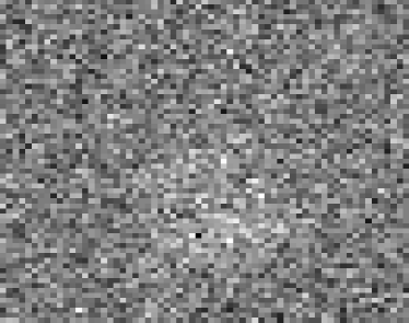
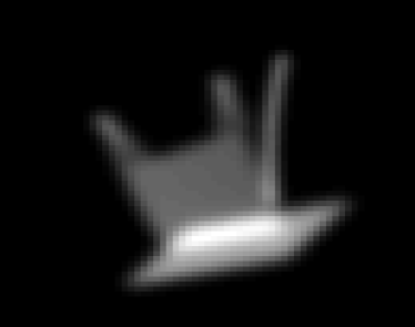
Figure 4: Sample of a noiseless projection image (right) and the same image with noise (left), as used in the simulation

In our preprocessing stage, we compute the Fourier transform of the image at sample points on concentric circles in the Fourier domain, and then use FFT to obtain the image coefficients on concentric circles defined in (44).

We run the algorithm ab initio, without an initial guess. We initialize the hyper-object to a non-heterogeneous spherically symmetric object, by setting each sphere to the average of the corresponding circles across all images, i.e. we set the $0$-th order coefficient in the expansion of the $k$-th shell to the normalized average of the $0$-th order coefficients $\alpha^{(i)}_{k,0}$ of the $k$-th circle of all the images.

We use SGD iterations to update the non-heterogeneous model object and after several steps of frequency marching we alternate between increasing the frequency limit $K$ and the number of parameterization basis functions $Q$.

For the purpose of visualization of the computed hyper-object, we choose sample values of the parameter $t$, and then sampled the shells at quadrature points in the Fourier domain and used NUFFT (see [36]) to recover each object at regular grid points in real space. We use Matlab’s “isosurface” and “patch” to visualize level sets of the objects.

The algorithm was run on computer equipped with Intel(R) Core(TM) i7-4770 CPU, 32GB RAM server and a single NVIDIA GeForce GTX 980 Ti GPU with 6 GB GPU RAM for about 5 hours. We note that very similar results have been obtained even in the 1-2 hours of this experiment and of similar shorter experiments.

Examples of reconstructed objects are presented in Figure 2. We observe that the reconstructed objects appear to be slightly rotated one with respect to the other compared to the simulated data, due to the ambiguity discussed in Section 4.6. In fact, the relative rotations in the result may reflect a better choice than our choice in the simulation, in terms of the rate of change in the hyper-object, or in terms of the norm of the heterogeneity coefficients.

In Figure 5, we present the distribution of the pairs of true-parameter (x-axis) and estimated parameter (y-axis) assigned to images during the final steps of the refinement, before the algorithm was stopped. This current simple implementation does not regularize or reparameterize the parameter space, and has been used ab initio, without any initial estimate; while it succeeds in obtaining an appropriate parameterization in the surprising majority of the runs, in some runs, typically when using a small number of iterations or very rapid frequency marching in early stages of the run, we find some examples of inefficient parameterization, which is typically not difficult to detect. For example, in Figure 6 we find that the algorithm maps most of the parameter space to extreme points, preliminary results suggest that even this naive implementation of the algorithm gradually reparameterizes this mapping, but this process is relatively slow. This incident is relatively easy to detect by examining the marginal distribution on the y-axis (under the assumption or constraint of a more uniform distribution). Another example, shown in Figure 7 demonstrates a way in which the algorithm can use only part of the allowed parameter space. The reconstruction results are still good in the region of space that the algorithms chose to use, but it is an inefficient use of the parameter space. This case is also easy to detect and correct. Conservative optimization appear to mitigate these issues even in the current implementation; initial estimates of the objects and better regularization are also likely to mitigate these issues when they occur.

Video visualizations of the results are available at the website
http://roy.lederman.name/cryo-em.

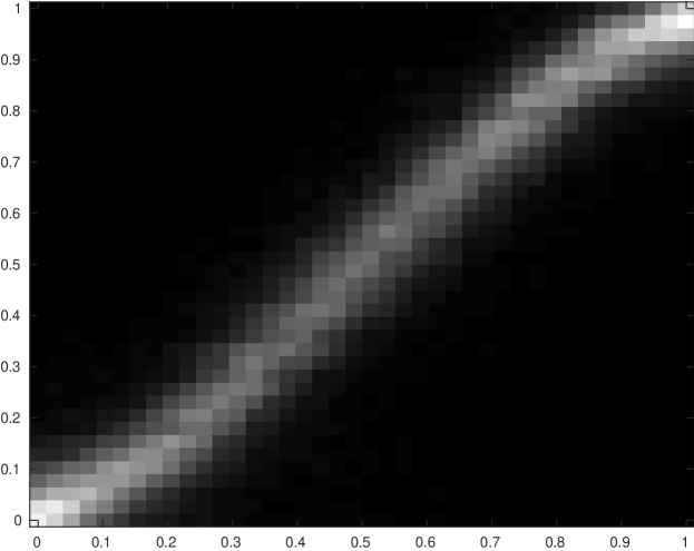
Figure 5: Distribution of the pairs true parameter values of an image (x-axis), and estimated parameter values (y-axis) in the parameterization that the algorithm finds, as assigned by the algorithm during the final iterations

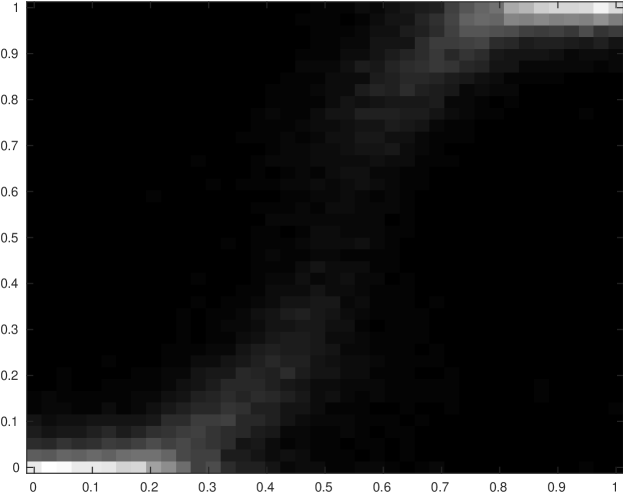
Figure 6: Distribution of the pairs true parameter values of an image, and estimated parameter values in the parameterization that the algorithm finds in an experiment with fewer iterations and more rapid marching. Here, the distribution is not uniform and only part of the heterogeneity is captured.

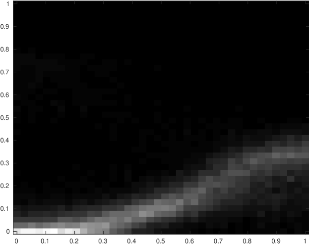
Figure 7: Distribution of the pairs true parameter values of an image, and estimated parameter values in the parameterization that the algorithm finds in another experiment with fewer iterations and more rapid marching. Here, only part of the parameter space is used.

7 Summary and future work

The idea behind this work is to extend the existing tools in cryo-EM to the case of continuous heterogeneity. Conceptually, we attempt to treat the heterogeneity parameter (or “class”) in the same way as the orientation. We propose various approaches for representing the heterogeneous hyper-objects and for regularizing the problem. In this manuscript, we presented one simple expansion of the hyper-object and one simple algorithm and implementation of these ideas as proof-of-concept. In this section we discuss some future directions for this line of work.

We believe that various versions of this general approach have several advantages compared to the construction of independent classes: it allows to use assumptions on the topology and properties of the heterogeneity in a given problem to improve the reconstruction, it captures the topology of the heterogeneous structures and provides a natural way to reconstruct object instances at arbitrary parameter points, it combines information from different nearby object instances to produce a fine-grained spectrum of states, leveraging continuity assumptions.

While many of the representation and regularization techniques proposed here can be implemented using sampled discretized values of the heterogeneity parameter, we find is particularly useful to use continuous bases in this discussion, because they offer a natural generalization of existing algorithms. In this manuscript we implemented only several continuous expansion using a tensor product of bases of functions and standard bases for the expansion of 3-D objects. More elaborate bases and other continuous and discrete representations of hyper-objects are likely to be useful in capturing properties of the heterogeneity and further development of this approach.

One possible source for methods that could be adapted, is the existing body of work in 4DCT. Since 4DCT typically treats the case where both the orientation and heterogeneity parameter value (phase in the breathing cycle) are known, not all the ideas in 4DCT are directly applicable. At the same time, the investigation of unknown parameters in cryo-EM may contribute to methods in CT, in cases where the breathing phase is not recorded accurately, or when there are additional heterogeneity parameters.

The examples used in this manuscript included only one dimensional heterogeneity on an interval, however the approach is general and can be used to investigate more elaborate topologies of heterogeneity. The investigation of other topologies and the sensitivity to the choice of topology, metrics, and bases is another direction in this line of work. We note that since the algorithms are relatively fast, it is possible to try multiple topologies, and we note that the tree/Haar approach is likely to be less sensitive to the precise choice of topology. However, the choice of topology is a useful implicit regularizer or prior. Another aspect of the work on topology is to develop methods of detecting local problems in the parameterizations that algorithms discover. While our discussion has been devoted mostly to continuous heterogeneity, the methods are applicable to discrete heterogeneity, for example when there are small changes between two conformations. A related matter that merits additional investigation is the case where some states in the continuum of states are far more represented than others, and the related issue of defining a metric on the space of heterogeneity.

The approach is general and we submit that it can be used in various existing cryo-EM algorithms (although the actual software implementations may require significant modifications). It is possible to combine existing software with this approach in several ways, for example, by crude continuous classification of images in this approach, followed by a local reconstruction, or a reconstruction of an initial homogeneous model of the molecule, and then superimposing local basis functions in areas of variability in the model and running this type of algorithm to resolve the heterogeneity.

While the results obtained using this preliminary prototype are promising, additional work is needed to complete the implementation of this approach in an algorithm that is efficient enough to reconstruct high resolution hyper-objects in real cryo-EM settings, while utilizing modest computational resources.

8 Conclusions

A framework has been presented for the tomography inverse problem in the case of continuously heterogeneous objects, where the orientation and heterogeneity parameter values are unknown. The proposed framework generalizes existing approaches for the reconstruction of molecules in cryo-EM, so that, in principal, existing algorithm can be adapted to the case of continuous heterogeneity.

The approach has been demonstrated in simplified simulated cryo-EM settings, using one of the proposed implementations, and a new prototype algorithm.

We are currently working on expanding our investigation of alternative representations and regularization approaches within this framework, and adapting the implementation to real-world cryo-EM applications.

References

- [1] A. Doerr, “Single-particle cryo-electron microscopy,” Nature Methods, vol. 13, no. 1, pp. 23–23, 2016.
- [2] E. Nogales, “The development of cryo-em into a mainstream structural biology technique,” Nature Methods, vol. 13, no. 1, pp. 24–27, 2016.
- [3] R. M. Glaeser, “How good can cryo-em become?,” Nature methods, vol. 13, no. 1, pp. 28–32, 2016.
- [4] D. A. Low, M. Nystrom, E. Kalinin, P. Parikh, J. F. Dempsey, J. D. Bradley, S. Mutic, S. H. Wahab, T. Islam, G. Christensen, et al., “A method for the reconstruction of four-dimensional synchronized ct scans acquired during free breathing,” Medical physics, vol. 30, no. 6, pp. 1254–1263, 2003.
- [5] R. R. Lederman and A. Singer, “A representation theory perspective on simultaneous alignment and classification,” arXiv preprint arXiv:1607.03464, 2016.
- [6] M. Abramowitz and I. Stegun, “Handbook of mathematical functions,” National Bureau of Standards, Applied Mathematics Series, vol. 55, p. 1046, 1964.
- [7] R. R. Coifman and G. Weiss, “Representations of compact groups and spherical harmonics,” Enseignement math, vol. 14, pp. 121–173, 1968.
- [8] A. Barnett, L. Greengard, A. Pataki, and M. Spivak, “Rapid solution of the cryo-em reconstruction problem by frequency marching,” arXiv preprint arXiv:1610.00404, 2016.
- [9] J. Frank, Three-dimensional electron microscopy of macromolecular assemblies: visualization of biological molecules in their native state. Oxford University Press, 2006.
- [10] M. Liao, E. Cao, D. Julius, and Y. Cheng, “Structure of the trpv1 ion channel determined by electron cryo-microscopy,” Nature, vol. 504, no. 7478, pp. 107–112, 2013.
- [11] M. Van Heel, “Angular reconstitution: a posteriori assignment of projection directions for 3d reconstruction,” Ultramicroscopy, vol. 21, no. 2, pp. 111–123, 1987.
- [12] A. Singer, R. R. Coifman, F. J. Sigworth, D. W. Chester, and Y. Shkolnisky, “Detecting consistent common lines in cryo-em by voting,” Journal of structural biology, vol. 169, no. 3, pp. 312–322, 2010.
- [13] A. Singer and Y. Shkolnisky, “Three-dimensional structure determination from common lines in cryo-em by eigenvectors and semidefinite programming,” SIAM journal on imaging sciences, vol. 4, no. 2, pp. 543–572, 2011.
- [14] Y. Shkolnisky and A. Singer, “Viewing direction estimation in cryo-em using synchronization,” SIAM journal on imaging sciences, vol. 5, no. 3, pp. 1088–1110, 2012.
- [15] S. H. Scheres, M. Valle, R. Nuñez, C. O. Sorzano, R. Marabini, G. T. Herman, and J.-M. Carazo, “Maximum-likelihood multi-reference refinement for electron microscopy images,” Journal of molecular biology, vol. 348, no. 1, pp. 139–149, 2005.
- [16] F. J. Sigworth, P. C. Doerschuk, J.-M. Carazo, and S. H. Scheres, “Chapter ten-an introduction to maximum-likelihood methods in cryo-em,” Methods in enzymology, vol. 482, pp. 263–294, 2010.
- [17] N. Grigorieff, “Frealign: high-resolution refinement of single particle structures,” Journal of structural biology, vol. 157, no. 1, pp. 117–125, 2007.
- [18] S. H. Scheres, “A bayesian view on cryo-em structure determination,” Journal of molecular biology, vol. 415, no. 2, pp. 406–418, 2012.
- [19] S. H. Scheres, “Relion: implementation of a bayesian approach to cryo-em structure determination,” Journal of structural biology, vol. 180, no. 3, pp. 519–530, 2012.
- [20] A. Punjani, M. Brubaker, and D. Fleet, “Building proteins in a day: Efficient 3d molecular structure estimation with electron cryomicroscopy,” IEEE Transactions on Pattern Analysis and Machine Intelligence, 2016.
- [21] A. Punjani, J. L. Rubinstein, D. J. Fleet, and M. A. Brubaker, “cryosparc: algorithms for rapid unsupervised cryo-em structure determination,” Nature Methods, vol. 14, no. 3, pp. 290–296, 2017.
- [22] N. Grigorieff, “Chapter eight-frealign: An exploratory tool for single-particle cryo-em,” Methods in enzymology, vol. 579, pp. 191–226, 2016.
- [23] D. Lyumkis, A. F. Brilot, D. L. Theobald, and N. Grigorieff, “Likelihood-based classification of cryo-em images using frealign,” Journal of structural biology, vol. 183, no. 3, pp. 377–388, 2013.
- [24] M. van Heel and M. Stöffler-Meilicke, “Characteristic views of e. coli and b. stearothermophilus 30s ribosomal subunits in the electron microscope.,” The EMBO journal, vol. 4, no. 9, p. 2389, 1985.
- [25] E. Katsevich, A. Katsevich, and A. Singer, “Covariance matrix estimation for the cryo-em heterogeneity problem,” SIAM journal on imaging sciences, vol. 8, no. 1, pp. 126–185, 2015.
- [26] J. Andén, E. Katsevich, and A. Singer, “Covariance estimation using conjugate gradient for 3d classification in cryo-em,” in Biomedical Imaging (ISBI), 2015 IEEE 12th International Symposium on, pp. 200–204, IEEE, 2015.
- [27] Y. Aizenbud and Y. Shkolnisky, “A max-cut approach to heterogeneity in cryo-electron microscopy,” arXiv preprint arXiv:1609.01100, 2016.
- [28] P. Schwander, R. Fung, and A. Ourmazd, “Conformations of macromolecules and their complexes from heterogeneous datasets,” Phil. Trans. R. Soc. B, vol. 369, no. 1647, p. 20130567, 2014.
- [29] J. Frank and A. Ourmazd, “Continuous changes in structure mapped by manifold embedding of single-particle data in cryo-em,” Methods, vol. 100, pp. 61–67, 2016.
- [30] X. Jia, Y. Lou, B. Dong, Z. Tian, and S. Jiang, “4d computed tomography reconstruction from few-projection data via temporal non-local regularization,” in International Conference on Medical Image Computing and Computer-Assisted Intervention, pp. 143–150, Springer, 2010.
- [31] H. Gao, R. Li, Y. Lin, and L. Xing, “4d cone beam ct via spatiotemporal tensor framelet,” Medical physics, vol. 39, no. 11, pp. 6943–6946, 2012.
- [32] D. Kazantsev, G. Van Eyndhoven, W. Lionheart, P. Withers, K. Dobson, S. McDonald, R. Atwood, and P. Lee, “Employing temporal self-similarity across the entire time domain in computed tomography reconstruction,” Phil. Trans. R. Soc. A, vol. 373, no. 2043, p. 20140389, 2015.
- [33] V. P. Gopi, P. Palanisamy, K. A. Wahid, P. Babyn, and D. Cooper, “Multiple regularization based mri reconstruction,” Signal Processing, vol. 103, pp. 103–113, 2014.
- [34] D. A. Low, P. J. Parikh, W. Lu, J. F. Dempsey, S. H. Wahab, J. P. Hubenschmidt, M. M. Nystrom, M. Handoko, and J. D. Bradley, “Novel breathing motion model for radiotherapy,” International Journal of Radiation Oncology* Biology* Physics, vol. 63, no. 3, pp. 921–929, 2005.
- [35] Y. Rubner, C. Tomasi, and L. J. Guibas, “The earth mover’s distance as a metric for image retrieval,” International journal of computer vision, vol. 40, no. 2, pp. 99–121, 2000.
- [36] L. Greengard and J.-Y. Lee, “Accelerating the nonuniform fast fourier transform,” SIAM review, vol. 46, no. 3, pp. 443–454, 2004.