A Hidden Markov Restless Multi-armed Bandit Model for Playout Recommendation Systems

Abstract

We consider a restless multi-armed bandit (RMAB) in which there are two types of arms, say A and B. Each arm can be in one of two states, say $0$ or $1.$ Playing a type A arm brings it to state $0$ with probability one and not playing it induces state transitions with arm-dependent probabilities. Whereas playing a type B arm leads it to state $1$ with probability $1$ and not playing it gets state that dependent on transition probabilities of arm. Further, play of an arm generates a unit reward with a probability that depends on the state of the arm. The belief about the state of the arm can be calculated using a Bayesian update after every play. This RMAB has been designed for use in recommendation systems where the user’s preferences depend on the history of recommendations. This RMAB can also be used in applications like creating of playlists or placement of advertisements. In this paper we formulate the long term reward maximization problem as infinite horizon discounted reward and average reward problem. We analyse the RMAB by first studying discounted reward scenario. We show that it is Whittle-indexable and then obtain a closed form expression for the Whittle index for each arm calculated from the belief about its state and the parameters that describe the arm. We next analyse the average reward problem using vanishing discounted approach and derive the closed form expression for Whittle index. For a RMAB to be useful in practice, we need to be able to learn the parameters of the arms. We present an algorithm derived from Thompson sampling scheme, that learns the parameters of the arms and also illustrate its performance numerically.

1 Introduction

Recommendations systems are used in almost all forms of modern media like YouTube and other video streaming services, Spotify and other music streaming services to create playlists. Playlists are also created on personal devices like digital music players. Highly personalised playlists are now being created using a variety of information that is mined from behavior history and social networking sites. A search for patents on playlist creation yields more than handful of items indicating a strong commercial interest in the search for good algorithm. The research literature though is scant.

A possible approach to create a playlist is to treat it as a ‘matrix completion’ problem, (e.g. [7], and choose a set of items from the completed matrix for which the user has a high preference.) A second approach would be to treat playlist creation as a recommendation system and generate a sequence of recommendations for the user. This is the view that we take in this paper but with the key of the user’s interest in items being influenced by immediate behavioral history. To the best of our knowledge such a system has not been considered in the literature. Specifically, we assume that user will like different items to be repeated at different rates and there will be some randomness in the preferences. The playlist creation system that we describe in this paper generates a dynamic list by taking a binary feedback from the user after an item has been played. Specifically, we allow different items to have different ‘return times’ in that some items may be played out more frequently than others.

We assume that the items are of two different categories—‘normal’ or type-A item and ‘viral’ or type-B item. For a normal item, the user preference goes from high low immediately after playing it and rises slowly after not playing it. The opposite is true for a ‘viral’ item, i.e., the preference goes to high immediately after play and decreases when it is not played. In this model, the recommendation system observes the user preference for the item only after playing it and not observed for other items. This feedback is accounted in subsequent plays of items. Since the user preferences are not observed for other items, system maintains the belief about the preference of the item. It is updated based on the action and outcome. The goal of system is to maximize a long term reward function. Such system can be modeled a restless multi-armed bandit (RMAB) with hidden states.

Typically, the users may have different preferences towards different items and also have different repetition rates. It may not be known at the beginning. Thus, the learning of associated state transition models and click through probabilities is required.

We next discuss the related literature on RMAB and learning in multi-armed bandits.

1.1 Related Literature

Typical recommendation system models based on multi-armed bandits take the form of contextual bandits, e.g., [15, 16]. A key feature in these models is that the user interests are assumed independent of the immediate recommendation history, i.e., the reward model is a static. We introduce the feature of making it dependent on the immediate recommendation history. Other models that address user reaction in recommendations use a finite sequence of past user responses as a basis for deciding the current recommendation, e.g., [13]; these are numerical studies and no provable properties are derived.

The classical stochastic multi-armed bandit problem for recommendation systems (RS) studied in [2, 6, 14], where RS chooses the items from given set of items at each time step. Play of an item yields a random reward that is drawn from probability distribution associated with item and it is unknown. There goal is to maximize the expected cumulative reward. This model do not have states associated with each item and rewards are drawn independently at each time step. It is studied as online learning problem. The performance is measured via regret, it is defined as difference between reward obtained using optimal strategy and reward obtained from strategy that is used for learning. A variant of stochastic multi-armed bandit considered in [8]. These are solved using efficient algorithms based on upper confidence bound (UCB). Further, it is shown that expected regret scales logarithmically with time steps. Recently, Thompson sampling (TS) based Bayesian algorithm considered for stochastic multi-armed in [1, 9, 11, 12]. In [9], authors have empirically illustrated the performance of Thompson sampling algorithm and observed that it performs better than UCB. TS algorithm is analysed in [1, 11] and shown that the regret scales logarithmically with number of time steps.

Another stochastic bandit, a restless multi-armed bandit first studied in seminal work of [29], where each arm has states associated with it and states evolve according to a Markov chain and that evolution is action dependent. Further, author proposed the heuristic index based policy, it is referred to as Whittle index policy. In [19, 22], we have considered a general system of a restless multi-armed bandit with unobservable states and action dependent transitions. In [22] we show that such a system is approximately Whittle-indexable. The restless bandit that we propose in this paper is a special case of that from [22] for which we can show exact Whittle indexability and also obtain a closed form expression for the Whittle index.

The standard restless multi-armed bandit work assumes that the transition probabilities and rewards are known. In recent work of [17], UCB based learning algorithm studied for a restless multi-armed bandit when transition probabilities and rewards are unknown. Also, Thompson sampling algorithm for a restless single armed bandit proposed and analysed in [20, 21]. In this paper, we also propose Thompson sampling based learning algorithm for RMAB and analyse its properties via numerical experiments.

1.2 Contributions

This paper is an extended version of [23]. Here, we extend our earlier work in [23] to long term average reward problem and discuss few variants of models. The detailed contributions from this paper are as follows.

1. We develop a restless multi-armed bandit (RMAB) model for use in recommendation systems and playlist creation. The arms of the bandit correspond to the items that may be recommended. Two types of arms may be defined—type $A$ and type $B.$ Each ‘like’ for a played arm yields a unit reward. We will seek a policy that maximises the infinite horizon discounted reward and a policy that maximises the long term average reward. The details are in Section 2.

2. We derive the value function properties for both type of arms in infinite horizon discounted reward and average reward. Using these properties, we obtain closed form expressions for value functions in Section 3.

3. We show that both types of arms are Whittle-indexable and obtain closed form expressions for the Whittle index. It is a function of the state of the arm. This is obtained for infinite horizon discounted reward case in Section 3.1. We also derive the expression for the Whittle index in average reward case, see Section 3.2.

4. The Whittle index policy is compared against a myopic policy in numerical experiments. We see that the index based policy indeed outperforms the myopic policy in many cases. This is covered in Section 4.

5. In Section 5 we discuss dual speed restless bandits for hidden states. For few variations of type A and type B arms, we obtain closed form expression of Whittle index.

6. Finally, in Section 6 we provide a Thompson sampling based algorithm for online learning of the parameters of the arms. A numerical comparison of the regret shows that the learning is effective.

We remark that the objective of the paper is not to design a recommendation system but to develop a new framework with provable properties for creating such systems.

2 Preliminaries and Model Description

To anchor the discussion, assume an automated playlist creation system (APCS) with $N$ items in its database. When an item is played, the user provides a binary feedback; a possible mechanism could be by clicking, or not clicking a ‘like’ button. The user’s interest in an item at any time is determined by an intrinsic interest and also on the time since it was last played. These features are captured in the model as follows. Each item in the database corresponds to one arm of the multi-armed bandit. The playout history of an arm is captured via a state variable for the arm and the interest in the item is captured via state-dependent ‘like’-probability for the arm. The state of each arm evolves independently of the other arms with transition probabilities that depend on whether it is played or not played.

We now formally describe the model. Time is measured in recommendation steps and is indexed by $t=1,2,3,\cdots,$ i.e., a recommendation is made in every step. $X_{t}(n)\in\{0,1\}$ is the state of arm $n$ at the beginning of step $t.$ $A_{t}(n)\in\{0,1\}$ is the action in step $t$ for arm $n$ with $A_{t}(n)=1$ corresponding to playing arm $n$ and $A_{t}(n)=0$ corresponding to not playing it. $X_{t}(n)$ evolves according to transition probabilities that depend on $A_{t}(n).$ There are two types of arms with arms in $\mathcal{A}=\{1,\ldots,M\}$ being type $A$ arms and those in $\mathcal{B}=\{M+1,\ldots,N\}$ being the type $B$ arms. $P_{ij}^{n}(a)$ denotes the transition probability from state $i$ to state $j$ for arm $n$ under action $a.$

For type $A$ arms, i.e., for $1\leq n\leq M,$ for $P_{00}^{n}(1)=1,$ $P_{10}^{n}(1):=1,$ $P_{01}^{n}(0):=p_{n},$ $P_{11}^{n}(0):=1$ Here, $p_{n}$ determines the preferred ‘repetition rate’ of arm $n.$ If $p_{n}$ is small, then the user prefers a large gap between successive times that the arm is played; if it is large then the preference is for smaller gaps. Type $A$ arms correspond to ‘normal’ items in that the user prefers sufficient gap between the playing of the item.

For type $B$ arms, i.e., for $M+1\leq n\leq N,$ the transition probabilities are $P_{01}^{n}(1)=1,$ $P_{11}^{n}(1)=1,$ $P_{00}^{n}(0)=1,$ $P_{10}^{n}(0)=p_{n}.$ Type $B$ arms correspond to ‘viral’ items where the preference is to have it played frequently and until it is ‘time to forget’ it. Thus $p_{n}$ determines the forgetting rate for a viral item.

When arm $n$ is played and it is in state $i,$ then a unit reward is accrued with probability $\rho_{n,i},$ $0<\rho_{n,i}<1.$ The reward corresponds to the user liking the playing of the arm and $\rho_{n,i}$ represents the intrinsic preference for the item. No reward is accrued from arms that are not played. The transition probabilities and rewards for the two types of arms are illustrated in Fig. 1 and Fig. 2.

State transitions and rewards when $A_{t}=0.$

State transitions and rewards when $A_{t}=1.$

Figure 1: Transition probabilities and reward structure for type-A arms

State transitions and rewards when $A_{t}=0.$

State transitions and rewards when $A_{t}=1.$

Figure 2: Transition probabilities and reward structure for type-B arms.

Observe that in the system, the state of an arm evolves even when it is not played; thus this is a restless multi-armed bandit. For each arm, we maintain a belief for the state of arm at the beginning of time step $t,$ denoted by $\pi_{t}(n),$ for arm $n.$ At the end of each time step, we can perform a Bayesian update of $\pi_{t}(n)$ using $p_{n}$ and $\rho_{n,i}$ along with the observation of the reward if the arm is played. We will define $\pi_{t}(n)=\mathsf{Pr}\left(X_{t}(n)=0\;\big{|}\;H_{t}\right).$ Here, $H_{t}$ denote the history of actions and observed rewards up to the beginning of time $t,$ i.e., $H_{t}\equiv(A_{s}(n),R_{s}(n))_{1\leq n\leq N,1\leq s<t},$ and $R_{t}(n)$ is the reward obtained in step $n$ from arm $n.$ One arm from the set of $N$ arms is to be played at each time step. Let $\phi=\{\phi(t)\}_{t>0}$ be the strategy where $\phi(t):H_{t}\to\{1,\ldots,N\}$ maps the history upto time $t$ to the action of playing one of the $N$ arms at time $t.$ Under the policy $\phi,$ let the action at time $t$ be denoted by

$$A^{\phi}_{t}(n)=\begin{cases}1&\mbox{if }\phi(t)=n,\\ 0&\mbox{if }\phi(t)\neq n.\end{cases}$$

The infinite horizon expected discounted reward under policy $\phi$ is given by

$$V_{\beta,\phi}(\pi):=\mathsf{E}\left({\sum_{t=1}^{\infty}\beta^{t-1}\bigg{(}\sum_{n=1}^{N}A^{\phi}_{t}(n)\ (\pi_{t}(n)\ \rho_{n,0}+\ \left.(1-\pi_{t}(n))\rho_{n,1}\right)\bigg{)}}\right).$$ (1)

Here $\beta$ is the discount factor, $0<\beta<1,$ the initial belief is $\pi(n)=\mathsf{Pr}\left(X_{1}(n)=0\right),$ and $\pi=[\pi(1),\cdots,\pi(N)]^{T}.$ The long term average reward under policy $\phi$ is given as follows.

$$V_{\phi}(\pi):=\lim_{T\rightarrow\infty}\frac{1}{T}\mathsf{E}\left({\sum_{t=1}^{T}\bigg{(}\sum_{n=1}^{N}A^{\phi}_{t}(n)\ (\pi_{t}(n)\ \rho_{n,0}+\ \left.(1-\pi_{t}(n))\rho_{n,1}\right)\bigg{)}}\right)$$ (2)

In this paper, our goal is in a policy $\phi$ that maximizes $V_{\beta,\phi}(\pi)$ for all $\pi\in[0,1]^{N}$ assuming that we know $p_{n},$ and $\rho_{n,i}$ for all $n.$ Similarly, in case of average reward problem we want to find a policy $\phi$ that maximizes $V_{\phi}(\pi)$ for all $\pi\in[0,1]^{N}.$

3 Towards the Whittle Index

As we have mentioned earlier, the problem (1) is a restless multi-armed bandit (RMAB) with partially observable states. In general, RMAB is computationally intractable. It is known to be $\mathrm{PSPACE}$-hard; see [24]. In light of this hardness, heuristic policies are sought. One class of heuristic policies is an index-based policy. Here, at the beginning of each time step, an index is calculated for each arm using the belief of the state of the arm, the transition probabilities and the reward probabilities and the arm(s) with highest index values are played in the step. A popular index-based policy is the Whittle-index policy based on a Lagrangian relaxation of (1). This was first outlined in [29]. In many cases, this policy is known to be asymptotically optimal; see [18],[10, Chapter $6$]. To be able to use this heuristic, we first need to show that each arm is indexable. To effectively use it, we need to derive the formulae to calculate the index. Indexability is proved by analysing a single arm. We first analyse a single armed bandit with infinite horizon discounted reward problem. Later, we will examine a single armed bandit with long term average reward problem.

3.1 Discounted reward problem

We begin by dropping the reference to $n,$ the sequence number of the arm to simplify the notation. Next, the arm is assumed to be assigned a subsidy $\lambda$ for not playing it. In view of this subsidy, (1) may be rewritten as follows.

$$V_{\beta}(\pi):=\mathsf{E}\left({\sum_{t=1}^{\infty}\beta^{t-1}\left(A_{t}^{\phi}\ (\pi_{t}\ \rho_{0}+(1-\pi_{t})\rho_{1})+\lambda(1-A_{t}^{\phi})\right)}\right).$$ (3)

Recall that $\pi_{t}=\mathsf{Pr}\left(X_{t}=0\;|\;H_{t}\right).$ For notational simplicity, we rewrite $A_{t}^{\phi}$ as $A_{t}$ with policy $\phi.$ The Bayesian updates for $\pi_{t}$ are obtained as follows.

• For a type $A$ arm: If $A_{t}=1,$ then $\pi_{t+1}=1$ and if $A_{t}=0,$ then $\pi_{t+1}=(1-p)\pi_{t}.$

• For a type $B$ arm: If $A_{t}=1,$ then $\pi_{t+1}=0$ and if $A_{t}=0,$ then $\pi_{t+1}=\pi_{t}+p(1-\pi_{t}).$

If $A_{t}=1,$ then the expected reward in the step is $\pi_{t}\rho_{0}+(1-\pi_{t})\rho_{1}.$ The policy $\phi(t):H_{t}\rightarrow\{0,1\},$ maps the history up to time $t,$ to an action $A_{t}$ in $t.$ From [25, 4, 5], the following is well known.

• $\pi_{t}$ captures the information in $H_{t},$ and is a sufficient statistic to construct policies that depend on the history.

• Optimal strategies can be restricted to stationary Markov policies.

• The optimum value function for fixed $\lambda$ and $\beta$, denoted $V_{\beta}(\pi,\lambda),$ is determined by solving the following dynamic program.

  $$V_{1,\beta}(\pi,\lambda) := \begin{cases}\pi\rho_{0}+(1-\pi)\rho_{1}+\beta V_{\beta}(1,\lambda)&\mbox{for type A}\\ \pi\rho_{0}+(1-\pi)\rho_{1}+\beta V_{\beta}(0,\lambda)&\mbox{for type B}\end{cases}$$

  $$V_{0,\beta}(\pi,\lambda) := \begin{cases}\lambda+\beta V_{\beta}((1-p)\pi,\lambda)&\mbox{for type A}\\ \lambda+\beta V_{\beta}(\pi+p(1-\pi),\lambda)&\mbox{for type B}\end{cases}$$

  $$V_{\beta}(\pi,\lambda) = \max\{V_{1,\beta}(\pi,\lambda),V_{0,\beta}(\pi,\lambda)\}.$$ (4)

  $V_{i,\beta}(\pi,\lambda)$ is the optimal value function if $A_{1}=i,$ $i=0,1.$

We next derive properties of the value functions $V_{\beta},$ $V_{0,\beta},$ and $V_{1,\beta}$ in the following Lemma.

Lemma 1

1. For fixed $\lambda$ and $\beta,$ $V_{\beta}(\pi,\lambda),$ $V_{0,\beta}(\pi,\lambda),$ $V_{1,\beta}(\pi,\lambda)$ are non-increasing convex in $\pi.$ Furthermore, $V_{1,\beta}(\pi,\lambda)$ is linear in $\pi.$

2. For fixed $\pi$ and $\beta,$ $V_{\beta}(\pi,\lambda),$ $V_{1,\beta}(\pi,\lambda)$ and $V_{0,\beta}(\pi,\lambda)$ are non-decreasing convex in $\lambda.$

3. For fixed $\pi$ and $\beta,$ $V_{1,\beta}(\pi,\lambda)$ and $V_{0,\beta}(\pi,\lambda)$ intersect at least once. This leads us to define (1) $\lambda_{L,\beta}$ such that for all $\lambda<\lambda_{L,\beta},$ the optimal action is to play the arm for all $\pi\in[0,1],$ and (2) $\lambda_{H,\beta}=\lambda_{H}$ such that for all $\lambda>\lambda_{H}$ the optimal action is to not play the arm for all $\pi\in[0,1].$ $\lambda_{L,\beta}$ and $\lambda_{H}$ are given as follows.

   $$\lambda_{H} = \begin{cases}\rho_{1}&\mbox{for type A,}\\ \rho_{1}&\mbox{for type B,}\end{cases}$$

   $$\lambda_{L,\beta} = \begin{cases}\rho_{0}+\beta q(\rho_{0}-\rho_{1})&\mbox{for type A,}\\ \rho_{1}+(1-\beta)(\rho_{0}-\rho_{1})&\mbox{for type B.}\end{cases}$$

The proof of Lemma 1 is analogous to the proofs in [22, Lemma $2$ and $3$]. Hence we omit the proof. In the next Lemma, we state the Lipschitz properties of value function with respect to $\pi$ and $\lambda.$

Lemma 2

1. For fixed $\lambda$ and $\beta,$ and $\forall\pi_{1},\pi_{2}\in[0,1],$ we have

   $$\big{|}V_{\beta}(\pi_{1},\lambda)-V_{\beta}(\pi_{2},\lambda)\big{|}\leq(\rho_{1}-\rho_{0})|\pi_{1}-\pi_{2}|$$

2. For fixed $\pi\in[0,1],$ and for $0<\beta<1,$
   

   $$\frac{\partial V_{\beta}(\pi,\lambda)}{\partial\lambda},\ \ \frac{\partial V_{1,\beta}(\pi,\lambda)}{\partial\lambda},\ \ \mbox{ and }\frac{\partial V_{0,\beta}(\pi,\lambda)}{\partial\lambda}$$

   are bounded above by $\frac{1}{1-\beta}.$

The proof is given in Appendix 0.A.1.

Remark 1

It is possible that $V_{\beta}(\pi,\lambda)$ is not differentiable with respect to $\pi$ or $\lambda.$ In that case the partial derivative of $V_{\beta}(\pi,\lambda)$ should be taken to be the right partial derivative. Note that such the right partial derivative exists because $V_{\beta}(\pi,\lambda)$ is convex in $\pi,$ $\lambda,$ and bounded.

Using the Lipschitz property of $V_{\beta}(\pi,\lambda)$ in $\pi,$ we derive the next result.

Lemma 3

For fixed $\lambda$ and $\beta,$ $V_{1,\beta}(\pi,\lambda)-V_{0,\beta}(\pi,\lambda)$ is decreasing in $\pi.$

The proof is detailed in Appendix 0.A.2. We now ready to present our first main result on a threshold policy structure.

Theorem 3.1 (Single threshold policy)

For the single-armed bandit, $0<\beta<1,$ and $\lambda_{L}\leq\lambda\leq\lambda_{H,\beta},$ the optimal policy is of threshold type with a single threshold. That is, there is a unique threshold $\pi_{T}\in[0,1]$ such that

$$V_{\beta}(\pi,\lambda)=\begin{cases}V_{1,\beta}(\pi,\lambda)&\mbox{if $\pi\leq\pi_{T},$ }\\ V_{0,\beta}(\pi,\lambda)&\mbox{if $\pi\geq\pi_{T},$ }\end{cases}$$

where $\pi_{T}=\{\pi\in[0,1]:V_{1,\beta}(\pi,\lambda)=V_{0,\beta}(\pi,\lambda)\}.$

Proof

Fix $\beta,\lambda.$ From Lemma 1 and 3, we have the following. For a fixed $\lambda,$ $V_{1,\beta}(\pi,\lambda)$ is linear in $\pi$ and $V_{0,\beta}(\pi,\lambda)$ is convex in $\pi.$ Also, $V_{1,\beta}(\pi,\lambda)-V_{0,\beta}(\pi,\lambda)$ is decreasing in $\pi.$ Thus there is at most one threshold. Furthermore, $V_{1,\beta}(\pi,\lambda)$ and $V_{0,\beta}(\pi,\lambda)$ intersect at least once for $\lambda_{L,\beta}\leq\lambda\leq\lambda_{H},$ $\pi\in[0,1].$ This completes the proof. ∎

Remark 2

1. The threshold policy implies that whenever belief at time step $t,$ $\pi_{t}$ is greater than $\pi_{T},$ then the optimal action is to not play the item.

2. For type-A arm, the belief about the state $0$ evolves to $(1-p)\pi_{t}$ when arm is not played. Thus, $\pi_{t+1}$ decreases whenever the item is not played and after some time steps, the optimal action will be to play the item. Once item is played, then $\pi_{t+1}$ reaches the state $0$ with probability $1.$ Let $K$ denotes the number of time steps to wait to play that item again and it depends on $\pi_{T},$ $\pi$ and $p.$ It is defined as follows.

   $$K(\pi,\pi_{T}):=\min\{k\geq 0:(1-p)^{k}\pi<\pi_{T}\}.$$

   Then,

   $$K(\pi,\pi_{T})=\begin{cases}0\ \ \ \ \ \ \ \ \ \ \ \ \ \ \ \ \ \ \ \ \ \ \ \mbox{if $\pi<\pi_{T},$ }\\ \left\lfloor{\frac{\log(\frac{\pi_{T}}{\pi})}{\log(1-p)}}\right\rfloor+1\ \ \ \ \ \mbox{ if $\pi\geq\pi_{T}$.}\end{cases}$$ (5)

   Using a threshold policy result and $K(\pi,\pi_{T}),$ we can derive the value function expressions as follows.

   $$V_{1,\beta}(\pi,\lambda) = \pi\rho_{0}+(1-\pi)\rho_{1}+\beta V_{0,\beta}(1,\lambda),$$

   $$V_{0,\beta}(\pi,\lambda) = \frac{\lambda\left(1-\beta^{K(\pi,\pi_{T})}\right)}{1-\beta}+\beta^{K(\pi,\pi_{T})+1}V_{0,\beta}(1,\lambda)+\beta^{K(\pi,\pi_{T})}\times$$

   $$\ \ \ \ \ \hskip 50.0pt\left(\rho_{1}+(\rho_{0}-\rho_{1})(1-p)^{K(\pi,\pi_{T})}\pi\right),$$

   $$V_{0,\beta}(1,\lambda) = \frac{\lambda(1-\beta^{K(1,\pi_{T})})}{\left(1-\beta^{K(1,\pi_{T})+1}\right)(1-\beta)}+\beta^{K(1,\pi_{T})}\frac{\left(\rho_{1}+(\rho_{0}-\rho_{1})(1-p)^{K(1,\pi_{T})}\right)}{\left(1-\beta^{K(1,\pi_{T})+1}\right)}.$$

3. For type-B arm, the belief about the state $0$ evolves to $\pi_{t}+p(1-\pi_{t})$ when arm is not played. Observe that $\pi_{t+1}$ is increases whenever arm is not played. Define $T(\pi):=\pi+p(1-\pi),$ $T^{k}(\pi)=T^{k-1}(T(\pi))$ and $\lim_{k\rightarrow\infty}T^{k}(\pi)=1.$ When a threshold $\pi_{T}\in(0,1],$ note that $V_{\beta}(0,\lambda)=V_{1,\beta}(0,\lambda)=\frac{\rho_{1}}{1-\beta}.$ Also, following holds.

   $$V_{\beta}(T(\pi),\lambda)=\begin{cases}V_{1,\beta}(T(\pi),\lambda)&\mbox{if $T(\pi)<\pi_{T},$}\\ V_{0,\beta}(T(\pi),\lambda)&\mbox{if $T(\pi)\geq\pi_{T}.$ }\end{cases}$$

   This discussion suggests that once that item is played, the user keeps liking that item. If the item is not played to the user, i.e. $\pi_{t}\geq\pi_{T}$, then the state of the item $\pi_{t}$ is always greater than $\pi_{T}$ for all $t$ and that means, that item is not played to the user at all. Thus the value function expressions are described below.

   $$V_{1,\beta}(\pi,\lambda) = \pi\rho_{0}+(1-\pi)\rho_{1}+\beta\frac{\rho_{1}}{1-\beta},$$

   $$V_{0,\beta}(\pi,\lambda) = \begin{cases}\lambda+\beta(\rho_{0}T(\pi)+(1-T(\pi))\rho_{1})+\beta\frac{\rho_{1}}{1-\beta}&\mbox{ if $T(\pi)<\pi_{T},$}\\ \frac{\lambda}{1-\beta}&\ \mbox{if $T(\pi)\geq\pi_{T},$}\end{cases}$$ (7)

   for $\pi_{T}\in(0,1].$ When $\pi_{T}=0,$ we have

   $$V_{1,\beta}(\pi,\lambda) = \pi\rho_{0}+(1-\pi)\rho_{1}+\beta\frac{\lambda}{1-\beta},$$

   $$V_{0,\beta}(\pi,\lambda) = \frac{\lambda}{1-\beta}.$$

From Theorem 3.1 and Remark 2, we can show the following.

Lemma 4

For fixed $\pi$ and $\beta,$ $V_{1,\beta}(\pi,\lambda)-V_{0,\beta}(\pi,\lambda)$ is a decreasing in $\lambda.$

The proof is given in Appendix 0.A.3. We first define indexability and later show that type-A and type-B arms are indexable. Define,

$$\mathcal{P}(\lambda) := \left\{\pi\in[0,1]:V_{1,\beta}(\pi,\lambda)\leq V_{0,\beta}(\pi,\lambda)\right\}$$

$\mathcal{P}(\lambda)$ is a set of all $\pi$ for which the optimal action is to not play the arm.

Definition 1 (Whittle indexability, [29])

An arm is Whittle indexable if $\mathcal{P}(\lambda)$ monotonically increases from $\emptyset$ to the entire state space $[0,1]$ as $\lambda$ increases from $-\infty$ to $\infty$, i.e., $\mathcal{P}(\lambda_{1})\setminus\mathcal{P}(\lambda_{2})=\emptyset$ whenever $\lambda_{1}<\lambda_{2}$. Further, a multi-armed bandit with $N$ arms is indexable if all arms are indexable.

We require the following result from [22, Lemma $4$] to prove Whittle indexability.

Lemma 5

Let $\pi_{T}(\lambda)=\inf\{0\leq\pi\leq 1:V_{S,\beta}(\pi,\lambda)=V_{NS,\beta}(\pi,\lambda)\}\in[0,1]$. If

$$\frac{\partial V_{1,\beta}(\pi,\lambda)}{\partial\lambda}\bigg{\rvert}_{\pi=\pi_{T}(\lambda)}\ <\ \frac{\partial V_{0,\beta}(\pi,\lambda)}{\partial\lambda}\bigg{\rvert}_{\pi=\pi_{T}(\lambda)},$$ (8)

then $\pi_{T}(\lambda)$ is a monotonically decreasing function of $\lambda.$

We next present our second main result.

Theorem 3.2 (Whittle indexable)

The single-armed bandit is indexable for $0<\beta<1$ and $\lambda_{L,\beta}\leq\lambda\leq\lambda_{H}.$

Proof

From Definition 1, it is clear that we have to show $\mathcal{P}(\lambda_{1})\subseteq\mathcal{P}(\lambda_{2})$ whenever $\lambda_{2}>\lambda_{1}.$ From Lemma 4, we note that $V_{1,\beta}(\pi,\lambda)-V_{0,\beta}(\pi,\lambda)$ is decreasing in $\lambda$ for fixed $\pi$ and $\beta.$ Therefore, (8) holds true. Using Lemma 5, $\lambda_{2}>\lambda_{1}$ implies $\pi_{T}(\lambda_{2})<\pi_{T}(\lambda_{1})$ for fixed $\beta.$ Hence, from the definition of the set $\mathcal{P}(\lambda),$ we get $\mathcal{P}(\lambda_{1})\subseteq\mathcal{P}(\lambda_{2})$ whenever $\lambda_{2}>\lambda_{1}.$ This completes the proof. ∎

We are now ready to define the Whittle index for an arm and provide an explicit formula for Whittle index in case of both type $A$ and type $B$ arms.

Definition 2 (Whittle index)

If an arm is indexable and is in state $\pi,$ then its Whittle index, $W(\pi),$ is

$$W(\pi) := \inf_{\lambda}\{\lambda:V_{1,\beta}(\pi,\lambda)=V_{0,\beta}(\pi,\lambda)\}.$$

$W(\pi)$ is the minimum subsidy $\lambda$ such that the optimal action is to not play the are at the given $\pi.$ To compute the Whittle index, we have to obtain the expressions of $V_{1,\beta}(\pi,\lambda)$ and $V_{0,\beta}(\pi,\lambda),$ equate them and solve it for $\lambda.$ After simplification, the Whittle index for type-A arm is as follows.

$$W(\pi)=\rho_{1}+\beta^{(K+1)}(\rho_{0}-\rho_{1})(1-p)^{K}+\frac{(\rho_{0}-\rho_{1})}{(1-\beta)}\left(1-\beta^{(K+1)}\right)\times\left[(1-\beta(1-p))\pi\right].$$

(9)

Here, $K=K(1,\pi)$ is waiting time before playing that arm again. Similarly, we can obtain the Whittle index formula for type-B arm, and it is

$$W(\pi) = \begin{cases}\rho_{1}+(1-\beta)(\rho_{0}-\rho_{1})\pi&\mbox{if $\pi\in(0,1],$}\\ \rho_{1}+(\rho_{0}-\rho_{1})\pi&\mbox{if $\pi=0.$}\end{cases}$$

Remark 3

Note that the Whittle index of an arm depends on model parameters $p,\rho_{0},\rho_{1},$ discount parameter $\beta,$ and belief $\pi.$

3.2 Average reward problem

We rewrite the average reward problem (2) in the view of subsidy $\lambda$ as follows.

$$V_{T,\phi}(\pi) := \mathsf{E}\left({\sum_{t=1}^{T}A^{\phi}_{t}\left(\pi_{t}\rho_{0}+(1-\pi_{t})\rho_{1}\right)+\lambda(1-A_{t}^{\phi})}\right),$$

$$V_{\phi}(\pi) = \max_{\phi}\lim_{T\rightarrow\infty}\frac{1}{T}V_{T,\phi}(\pi).$$ (11)

Here, $A^{\phi}(t)=i$ if $\phi(t)=i,$ $i\in\{0,1\},$ $\pi_{1}=\pi.$ It is solved by the vanishing discount approach [3, 26]—by first considering a discounted reward system and then taking limits as the discount approaches to $1.$ Define

$$\overline{V}_{\beta}(\pi,\lambda):=\begin{cases}V_{\beta}(\pi,\lambda)-V_{\beta}(1,\lambda)&\mbox{for type-A arm,}\\ V_{\beta}(\pi,\lambda)-V_{\beta}(0,\lambda)&\mbox{for type-B arm,}\end{cases}$$

for $\pi\in[0,1].$ Using Eqn. (4), we can obtain for type-A arm

$$\overline{V}_{\beta}(\pi,\lambda)+(1-\beta)V_{\beta}(1,\lambda) = \max\left\{\lambda+\beta\overline{V}_{\beta}((1-p)\pi,\lambda),\pi\rho_{0}+(1-\pi)\rho_{1}\right\},$$

and for type-B arm

$$\overline{V}_{\beta}(\pi,\lambda)+(1-\beta)V_{\beta}(0,\lambda) = \max\left\{\lambda+\beta\overline{V}_{\beta}(\pi+p(1-\pi),\lambda),\pi\rho_{0}+(1-\pi)\rho_{1}\right\}.$$

From Lemma 1, $\overline{V}_{\beta}(\pi,\lambda)$ is a convex monotone function in $\pi$ for fixed $\lambda$ and $\beta.$ By definition of $\overline{V}_{\beta}(\pi,\lambda)$ we have $\overline{V}_{\beta}(1,\lambda)=0$ for type-A and $\overline{V}_{\beta}(0,\lambda)=0$ for type-B arm. Further, from Lemma 2, we know that there is a constant $C<\infty$ such that $\big{|}V_{\beta}(\pi,\lambda)-V_{\beta}(1,\lambda)\big{|}<C$ for fixed $\beta$ and $\lambda\in[-\rho_{1},\rho_{1}].$ This implies that $\overline{V}_{\beta}(\pi,\lambda)$ is bounded and Lipschitz-continuous. Finally, $(1-\beta)V_{\beta}(\pi,\lambda)$ is also bounded. Hence we can apply the Arzela-Ascoli theorem [28], to find a subsequence $(\overline{V}_{\beta_{k}}(\pi,\lambda),(1-\beta_{k})V_{\beta_{k}}(\pi,\lambda))$ that converges uniformly to $(V(\pi,\lambda),g)$ as $\beta_{k}\rightarrow 1.$ Thus, as $\beta_{k}\rightarrow 1,$ along an appropriate subsequence, (LABEL:eqn:V-bar-of-beta-1) reduces to

$$V(\pi,\lambda)+g=\max\left\{\lambda+V((1-p)\pi,\lambda),\pi\rho_{0}+(1-\pi)\rho_{1}\right\},$$ (14)

and (LABEL:eqn:V-bar-of-beta-2) reduces to

$$V(\pi,\lambda)+g=\max\left\{\lambda+V(\pi+p(1-\pi),\lambda),\pi\rho_{0}+(1-\pi)\rho_{1}\right\}.$$ (15)

Equation (14) and (15) are the dynamic programming equations for type-A and type-B arm in case of average reward system. Hence it is the optimal solution of (11).
Also, note that $V(\pi,\lambda)$ inherits the structural properties of $V_{\beta}(\pi,\lambda).$ From Lemma 1 and Theorem 3.1, we obtain next result.

Lemma 6

1. For fixed $\lambda,$ $V(\pi,\lambda)$ is a monotone non-increasing and convex in $\pi.$

2. The optimal policy is a single threshold type for $\lambda\in[\lambda_{L},\lambda_{H}],$ where $\lambda_{H}=\rho_{1}$ and

   $$\lambda_{L} = \begin{cases}\rho_{0}+p(\rho_{0}-\rho_{1})&\mbox{for type A,}\\ \rho_{1}&\mbox{for type B.}\end{cases}$$

This in turn leads us to the following theorem which is a direct analog of Theorem 6.17 in [26].

Theorem 3.3

If there exists a bounded function $V(\pi,\lambda)$ for $\pi\in[0,1],$ $\lambda\in[\lambda_{L},\lambda_{H}]$ and a constant $g$ that satisfies equation (14), (15) then there exists a stationary policy $\phi^{*}$ such that

$$g = \max_{\phi}\lim_{T\rightarrow\infty}\frac{1}{T}V_{T,\phi}(\pi,\lambda)$$ (16)

$$\phi^{*} = \arg\max_{\phi}\lim_{T\rightarrow\infty}\frac{1}{T}V_{T,\phi}(\pi,\lambda).$$ (17)

for all $\pi\in[0,1],$ fixed $\lambda,$ and moreover, $\phi^{*}$ is the policy for which the RHS of (14),(15) is maximized.

We next derive the Whittle index formula. From Lemma 5, recall that to claim indexability, we have shown that $\pi_{T}(\lambda)$ is a monotonically decreasing in $\lambda$ for discounted reward case. Similarly, in average reward case, we require to show this claim. From Arzela-Ascoli theorem, we know that $V(\pi,\lambda)$ inherits the properties of $V_{\beta}(\pi,\lambda).$ Thus, $\pi_{T}(\lambda)$ is a monotonically decreasing in $\lambda$ for $\beta=1.$ Then we can show that an arm is indexable. Further, the index can be evaluated by letting $\beta\rightarrow 1$ in the Whittle index formula of discounted case. Hence from equation (9) and (LABEL:eq:whittle-index-B), we obtain the Whittle index formula.

• For type-A arm:

  $$W(\pi)=\rho_{1}+(\rho_{0}-\rho_{1})(1-p)^{K}+K(\rho_{0}-\rho_{1})\left[(1-(1-p))\pi\right].$$

  (18)

  Here, $K=K(1,\pi)$ is waiting time before playing that arm again.

• For type-B arm:

  $$W(\pi) = \rho_{1}.$$ (19)

4 Numerical Results: Whittle index and Myopic Algorithm

  Input: $N$ arms, initial belief $\pi=\left[\pi(1),\cdots,\pi(N)\right],$ $\pi_{1}=\pi,$

  repeat

     for $n=1,\ldots,N$ do

        Compute $W(\pi(n))$

     end for

     Evaluate $i=\arg\max_{1\leq n\leq N}W(\pi(n)).$

     Play arm $i$

     if  $i$ is Type A then

        $\pi_{t+1}(i)=1$

     end if

     if $I$ is Type B then

        $\pi_{t+1}(i)=0$

     end if

     for $n=1,\ldots,M,$ $n\neq i$ do

        $\pi_{t+1}(n)=(1-p_{n})\pi_{t}(n),$

     end for

     for $n=M+1,\ldots,N,$ $n\neq i$ do

        $\pi_{t+1}(n)=(1-p_{n})\pi_{t}(n)+p_{n},$

     end for

  until forever

Algorithm 1 Whittle index algorithm for APCS with type $A$ and type $B$ arms.

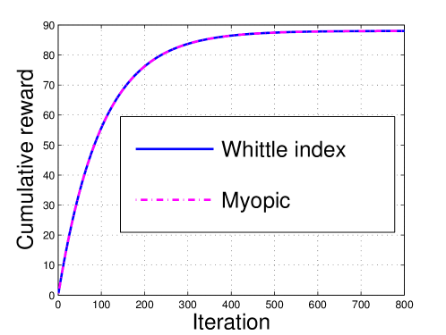
(a)

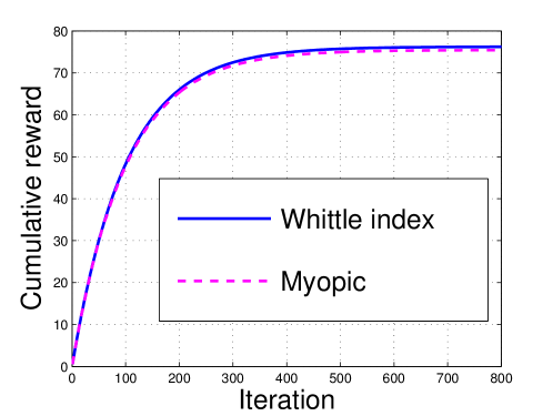
(b)

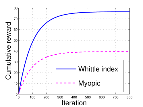
(c)

Parameters

	$\rho_{0}$	$\rho_{1}$	$p$
(a)	$[0.07,0.04,0.05,0.12,0.99]$	$[0.71,0.85,0.77,0.76,0.88]$	$[0.09,0.23,0.23,0.12,0.27]$
(b)	$[0.02,0.02,0.11,0.16,0.19]$	$[0.64,0.77,0.74,0.60,0.76]$	$[0.06,0.24,0.10,0.16,0.15]$
(c)	$[0.07,0.09,0.01,0.19,0.04]$	$[0.63,0.71,0.66,0.75,0.77]$	$[0.29,0.28,0.03,0.22,0.18]$

Figure 3: Cumulative reward vs time for $N=5$ with APCS having both types of arms.

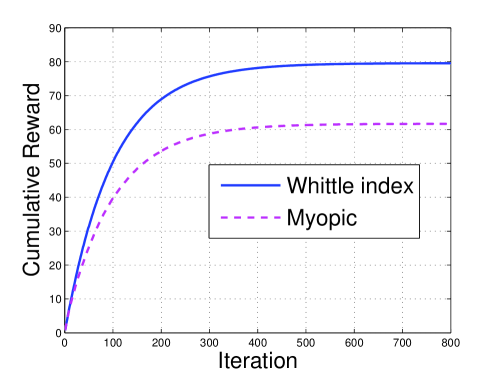
(a)

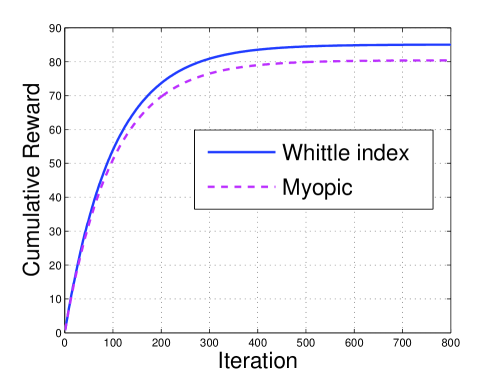
(b)

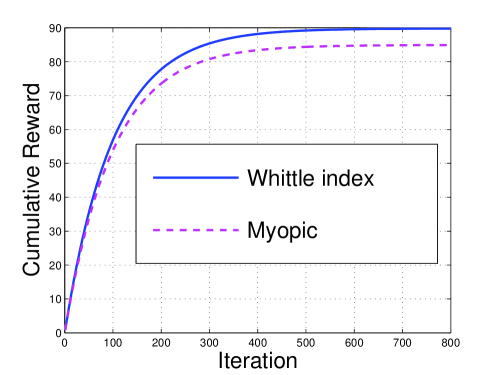
(c)

Figure 4: Cumulative reward vs time for different $N$ with APCS having both types of arms.

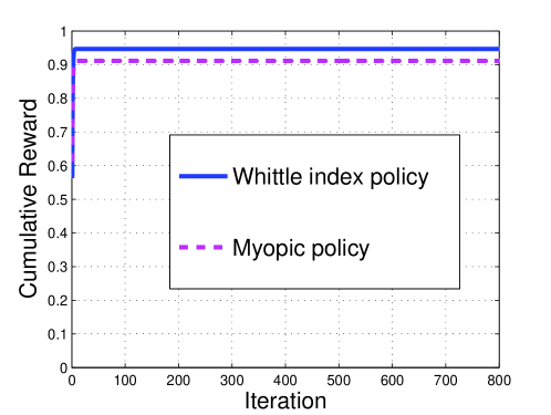
(a)

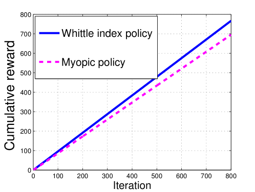
(b)

Figure 5: Cumulative reward vs time for $\beta=0.3,1$ and $N=200$ with APCS having both types of arms. Fig. 5a $\beta=0.3$ and Fig. 5b $\beta=1.$

In this section we present some numerical results to illustrate the performance of the Whittle index based recommendation algorithm. The simulations use Algorithm 1. We compare the performance of Whittle index based algorithm against that of a myopic algorithm that plays the arm that has the highest expected reward in the step. We consider small size ($N=5,10$), medium size ($N=20$), and large size ($N=100$) systems. For all the cases we use $\beta=0.99.$

In Fig. 3, we present numerical examples when there are a small number of arms, i.e., $N=5.$ In this case, arms 1–4 are of type $A$ and arm $5$ is of type $B$ arm. The system is simulated for parameter sets which are also shown in the figure. In all the cases, the initial belief used is $\pi=[0.4,0.4,0.4,0.4,0.4].$ In the first system $\rho_{0}$ and $\rho_{1}$ for the type $B$ arm are close to one and both policies almost always choose that arm. Hence their performances are also comparable. This is seen in Fig 3(a). The behavior is similar even when the $\rho_{1}$s of all the arms are comparable as in the second system with performance shown in Fig. 3(b). In this system, in the 800 plays, the type $B$ arm was played 28 and 75 times in the Whittle index and the myopic systems respectively. In the third small system, the Whittle index system plays the type $B$ arms significantly more frequently than the myopic system and has a significantly better performance; this is shown in Fig. 3c.

Fig. 4 shows the performance of the two systems for larger systems. These are obtained as follows. For $N=10,$ we have nine type $A$ arms and one type $B$ arm. For $N=50,$ we use $48$ type $A$ arms and $2$ type $B$ arms. The system with $N=200,$ has $190$ type $A$ arms and $10$ type $B$ arms. We generate reward and transition probabilities randomly using the formula $\rho_{0}=0.01+0.19*\mathrm{rand}(1,N),$ $\rho_{1}=0.6+0.3*\mathrm{rand}(1,N),$ $p=0.01+0.29*\mathrm{rand}(1,N).$ The initial belief $\pi=0.4*\mathrm{ones}(1,N).$ We observe that the Whittle index algorithm some gain the over myopic algorithm but the gain decreases with increasing $N.$ The decrease is due because with large $N,$ the waiting time for each item is large and this causes many arms to be in state $1$ with high probability.

In Fig. 5, we compare the performance of two systems for different values of discount parameter $\beta=0.3,1$ and $N=200.$ We notice that even for small $\beta=0.3,$ the Whittle index algorithm gains over myopic algorithm.

5 Variants of type A and type B arms

Here, we mention few extensions of a hidden RMAB. By considering different structure on transition probabilities, we can obtain different type of arms and models.

• We consider few variants of type A and type B arms that generalized our current model. The transition probabilities for this model are as follows.

  $$P_{01}^{n}(0)=p_{n},\ \ P_{10}^{n}(0)=q_{n}$$ for both type arm,

  $$P_{01}^{n}(1)=\begin{cases}\epsilon P_{01}^{n}(0)&\ \mbox{if arm is type A,}\\ (1-\epsilon)+\epsilon P_{01}^{n}(0)&\ \mbox{if arm is type B,}\\ \end{cases}$$

  $$P_{10}^{n}(1)=\begin{cases}(1-\epsilon)+\epsilon P_{10}^{n}(0)&\ \mbox{if arm is type A,}\\ \epsilon P_{10}^{n}(0)&\ \mbox{if arm is type B,}\\ \end{cases}$$

  for $\epsilon\in[0,1).$ This may be thought as the arm evolving with different speeds under actions $1$ and $0.$ This is referred to dual speed restless bandit in [10, Chapter $6,$ Secion $6.2$].

• Notice that for $\epsilon=0,$ current model leads to a simple variant of type A and type B arm. For this model, we can derive all properties of value functions as in Section 3 using similar approach. Also, the Whittle index formula can be obtained. This is given in next subsection.

• For $\epsilon\in(0,1),$ difficulty level of problem increases significantly because the current belief about state, $\pi_{t+1}(n)$ becomes non linear function of previous belief $\pi_{t}(n)$ when arm $n$ is played. Thus, it is hard to show that the arm is Whittle-indexable. But the approximate Whittle-indexability is proved in [22] under restriction on discount parameter $\beta.$

5.1 A simple variant of the current model

In this, we suppose $\epsilon=0,$ and derive the value function expressions, and Whittle index expression. To obtain these, we consider a single arm restless bandit. In such setting, we have transition probabilities as follows. $P_{01}(0)=p,$ $P_{10}(0)=q$ for both type arm, and

$$P_{01}^{n}(1)=\begin{cases}0&\ \mbox{if arm is type A,}\\ 1&\ \mbox{if arm is type B,}\\ \end{cases}$$

$$P_{10}^{n}(1)=\begin{cases}1&\ \mbox{if arm is type A,}\\ 0&\ \mbox{if arm is type B.}\\ \end{cases}$$

We first provide analysis for type A arm and then for type B arm.

1. Type A arm: The dynamic programming equation for discounted reward system is

   $$V_{\beta}(\pi,\lambda) = \max\{V_{0,\beta}(\pi,\lambda),V_{1,\beta}(\pi,\lambda)\},$$

   $$V_{0,\beta}(\pi,\lambda) = \lambda+\beta V_{\beta}(\gamma(\pi),\lambda),$$

   $$V_{1,\beta}(\pi,\lambda) = \pi\rho_{0}+(1-\pi)\rho_{1}+\beta V_{\beta}(1,\lambda)),$$

   where $\gamma(\pi)=\pi(1-p)+(1-\pi)q.$ We also assume that $p+q\leq 1.$ Define $\gamma^{k}(\pi):=\gamma^{k-1}(\gamma(\pi)).$ Note that as $\lim_{k\rightarrow\infty}\gamma^{k}(\pi)=\gamma_{\infty},$ where $\gamma_{\infty}=\frac{q}{q+p}.$ Also observe that as $\pi>\gamma_{\infty},$ then $\gamma^{k}(\pi)$ is decreases to $\gamma_{\infty}$ with $k$ and if $\pi<\gamma_{\infty}$ then $\gamma^{k}(\pi)$ is increases to $\gamma_{\infty}$ with $k.$
   Mimicking the proof technique in Section 3, we can show that the optimal policy is of a threshold type and arm is Whittle indexable. Now using threshold policy result, we can derive the closed form expressions for value functions.

   $$K(\pi,\pi_{T}):=\min\{k\geq 0:\gamma^{k}(\pi)<\pi_{T}\}.$$

   Then

   $$K(\pi,\pi_{T})=\begin{cases}0\ \ \ \ \ \ \ \ \ \ \ \ \ \ \ \ \ \ \ \ \ \ \ \mbox{if $\pi<\pi_{T},$ }\\ \left\lfloor{\frac{\log(\pi_{T})}{\log(\gamma(\pi))}}\right\rfloor+1\ \ \ \ \ \mbox{ if $\pi\geq\pi_{T}$.}\end{cases}$$

   To obtain value function expressions, we consider two cases.

   • When $\pi_{T}\in[0,\gamma_{\infty}),$ $K(1,\pi_{T})=\infty$ because $\gamma^{k}(\pi)$ is decreasing to $\gamma_{\infty}$ and this will never cross a threshold $\pi_{T}$ for finite $k.$ Also, from Theorem 3.1, we can have

     $$V_{0,\beta}(1,\lambda) = \lambda+\beta V_{0,\beta}(\gamma(1),\lambda)$$

     $$= \lambda+\beta\lambda+\beta^{2}V_{0,\beta}(\gamma^{2}(1),\lambda).$$

     And $\lim_{k\rightarrow\infty}\gamma^{k}(1)=\gamma_{\infty}.$ Expanding recursion of $V_{0,\beta}(\gamma^{k}(1),\lambda)$ we obtain

     $$V_{0,\beta}(1,\lambda) = \frac{\lambda}{1-\beta}.$$

     $$V_{1,\beta}(\pi,\lambda) = \pi\rho_{0}+(1-\pi)\rho_{1}+\beta\frac{\lambda}{1-\beta}.$$

     Note that $\pi\geq\pi_{T},$ $\gamma^{k}(\pi)\geq\pi_{T}$ for any $k\geq 1.$ Thus

     $$V_{0,\beta}(\pi,\lambda) = \begin{cases}\lambda+\beta\bigg{(}\gamma(\pi)\rho_{0}+(1-\gamma(\pi))\rho_{1}\bigg{)}+\beta^{2}\frac{\lambda}{1-\beta}&\mbox{if $\gamma(\pi)<\pi_{T},$}\\ \frac{\lambda}{1-\beta}&\mbox{if $\gamma(\pi)\geq\pi_{T}.$}\end{cases}$$

   • When $\pi_{T}\in[\gamma_{\infty},1],$ we have $K(1,\pi_{T})<\infty.$ Using a threshold policy result and after simplification we get

     $$V_{0,\beta}(1,\lambda) = \frac{\lambda\left(1-\beta^{K(1,\pi_{T})}\right)}{\left(1-\beta^{(K(1,\pi_{T})+1)}\right)(1-\beta)}+\beta^{K(1,\pi_{T})}\frac{\rho(\gamma^{K(1,\pi_{T})}(1))}{\left(1-\beta^{(K(1,\pi_{T})+1)}\right)},$$

     $$V_{0,\beta}(\pi,\lambda) = \frac{\lambda\left(1-\beta^{K(\pi,\pi_{T})}\right)}{(1-\beta)}+\beta^{K(\pi,\pi_{T})}\rho\left(\gamma^{K(\pi,\pi_{T})}(\pi)\right)+\beta^{\left(K(\pi,\pi_{T})+1\right)}V_{0,\beta}(1,\lambda)$$

     $$V_{1,\beta}(\pi,\lambda) = \rho(\pi)+\beta V_{0,\beta}(1,\lambda).$$

     where $\rho(\pi)=\pi\rho_{0}+(1-\pi)\rho_{1}.$

   We now derive expressions for the Whittle index. When $\pi\in[0,\gamma_{\infty}),$ the Whittle index is

   $$W(\pi)=\pi\rho_{0}+(1-\pi)\rho_{1}.$$

   When $\pi\in[\gamma_{\infty},1]$ the Whittle index is

   $$W(\pi)=\rho_{1}+\beta^{\left(K(1,\pi)+1\right)}(\rho_{0}-\rho_{1})\gamma^{K(1,\pi)}(1)+\frac{(\rho_{0}-\rho_{1})}{(1-\beta)}\left(1-\beta^{(K(1,\pi)+1)}\right)\left(\pi-\beta\gamma(\pi)\right).$$

   Using the vanishing discounted approach, we can analyse average reward problem and for that we can obtain the Whittle index expression by letting discount parameter $\beta$ approach $1.$ Hence

   $$W(\pi) = \begin{cases}\pi\rho_{0}+(1-\pi)\rho_{1}&\mbox{if $\pi\in[0,\gamma_{\infty})$}\\ \rho_{1}+(\rho_{0}-\rho_{1})\gamma^{K}(1)+K(\rho_{0}-\rho_{1})\left(\pi-\beta\gamma(\pi)\right)&\mbox{if $\pi\in[\gamma_{\infty},1]$}\end{cases}$$

   where $K=K(1,\pi).$
   

2. Type B arm: The dynamic programming equation for discounted reward is as follows.

   $$V_{\beta}(\pi,\lambda) = \max\{V_{1,\beta}(\pi,\lambda),V_{0,\beta}(\pi,\lambda)\},$$

   $$V_{1,\beta}(\pi,\lambda) = \pi\rho_{0}+(1-\pi)\rho_{1}+\beta V_{\beta}(0,\lambda),$$

   $$V_{0,\beta}(\pi,\lambda) = \lambda+\beta V_{\beta}(\gamma(\pi),\lambda).$$

   We now obtain the value function expressions. For $\pi_{T}\in(0,1],$ we can get

   $$V_{1,\beta}(0,\lambda) = \rho_{1}+\beta V_{1,\beta}(0,\lambda)$$

   Hence after simplification we have

   $$V_{1,\beta}(0,\lambda) = \frac{\rho_{1}}{1-\beta},$$

   $$V_{1,\beta}(\pi,\lambda) = \pi\rho_{0}+(1-\pi)\rho_{1}+\beta\frac{\rho_{1}}{1-\beta}.$$

   If $\pi_{T}\in(0,\gamma_{\infty})$ then

   $$V_{0,\beta}(\pi,\lambda)=\begin{cases}\lambda+\beta\rho(\gamma(\pi))+\beta^{2}\frac{\rho_{1}}{1-\beta}&\mbox{if $\pi<\pi_{T},$}\\ \frac{\lambda}{1-\beta}&\mbox{if $\pi\geq\pi_{T}.$}\end{cases}$$

   If $\pi_{T}\in[\gamma_{\infty},1],$ then

   $$V_{0,\beta}(\pi,\lambda)=\begin{cases}\frac{\lambda(1-\beta^{K(\pi,\pi_{T})})}{1-\beta}+\beta^{K(\pi,\pi_{T})}\left(\rho(\gamma^{K(\pi,\pi_{T})}(\pi))+\beta\frac{\rho_{1}}{1-\beta}\right)&\mbox{if $\pi<\pi_{T},$}\\ \lambda+\beta\rho(\gamma(\pi))+\beta^{2}\frac{\lambda}{1-\beta}&\mbox{if $\pi>\pi_{T},$}\\ \frac{\lambda}{1-\beta}&\mbox{if $\pi=\pi_{T}.$}\end{cases}$$

   For $\pi_{T}=0$ we can obtain

   $$V_{1,\beta}(\pi,\lambda) = \pi\rho_{0}+(1-\pi)\rho_{1}+\beta\frac{\lambda}{1-\beta},$$

   $$V_{0,\beta}(\pi,\lambda) = \frac{\lambda}{1-\beta}.$$

   The Whittle index expression is given as.

   $$W(\pi) = \begin{cases}\rho_{1}&\mbox{for $\pi=0,$}\\ (1-\beta)(\pi\rho_{0}+(1-\pi)\rho_{1})+\beta\rho_{1}&\mbox{for $\pi\in(0,1].$}\end{cases}$$

For average reward, the Whittle index in this model is same as (19).

6 Thompson-Sampling Based Learning

The key to a useful use of the model from the preceding sections is the knowledge of the parameters. These are not known a priori in most systems. In this section, we describe an algorithm that learns the parameters from the available feedback. Our scheme is a version of Thompson sampling [27] which has been studied for stochastic multi-armed bandits [1, 12], learning in Markov decision processes (MDPs) [11] and in POMDPs [21]. In fact our algorithm is an extension of the scheme for the one-armed bandit, modeled as a POMDP, that was described and analysed in [21]. An important requirement of the learning algorithm is to have a low regret, i.e., the exploration and exploitation sequences should be cleverly mixed to ensure that the difference between the ideal and the realised objective functions are small. In [21] we formally show that the regret is logarithmic for the one-armed case. The algorithm for the multi-armed case is described in Algorithm 2, and we expect that its performance is also good. A formal analysis is being worked out.

The algorithm proceeds as follows. At the beginning, we initialize a prior distribution on the space of all candidate parameters models, which in our case is a subset $\Theta_{i}$ of the unit cube $[0,1]^{3};$ $\Theta_{i}$ contains all possible models for the parameters $\theta_{i}$ of arm $i.$ In each step, assume that the true values of the parameters are $\theta_{i}$ and use the Whittle index (or the myopic) algorithm to choose the arm that is to be played. Recall that the arm with highest index is played in the Whittle index algorithm and the arm with highest expected reward is played in myopic algorithm. The playing of the arm $A_{t}$ at time $t$ yields a payoff $R_{t}.$ This is used to update the prior distribution $Z_{i}$ of the parameter space for that arm. This update is performed using Bayes’ rule and the observed reward. The model distribution for the other arms remain unchanged. We explain the update mechanism next. Let $\mathcal{B}({\Theta}_{i})$ denote the Borel $\sigma$-algebra of $\Theta_{i}\subset[0,1]^{3}$ for the arms indexed by $i=1,\ldots,N.$ Let $\mathsf{Pr}\left(R=r\;\big{|}\;\theta,A\right)$ denote the likelihood, under the model $\theta$, of observing a reward of $r\in\{0,1\}$ upon action $A\in\{1,\cdots,N\}.$ This likelihood can be seen to be as follows.

$$\mathsf{Pr}\left(R=r\;\big{|}\;\theta,A=i\right)=\begin{cases}f(\theta_{i},i)&\mbox{if $r=1,$}\\ 1-f(\theta_{i},i)&\mbox{if $r=0.$}\end{cases}$$

Here $f(\theta_{i},i)$ is the probability of observing a reward of $1$ after playing arm $i$ when the parameter is $\theta_{i}.$ Letting $k_{i}$ denote the number of time steps since the last time that arm $i$ was played, we can obtain $f(\theta_{i},i)$ as follows.

$$f(\theta_{i},i)=\begin{cases}(1-p_{i})^{k_{i}}\rho_{i,0}+(1-(1-p_{i})^{k_{i}})\rho_{i,1},&\mbox{if $i$ is type A arm, }\\ (1-(1-p_{i})^{k_{i}})\rho_{i,0}+(1-p_{i})^{k_{i}}\rho_{i,1},&\mbox{if $i$ is type B arm.}\end{cases}$$

This likelihood is used to update the prior distribution $Z_{i,t}$ and the parameters of the arm is selected from this distribution. We reiterate that the parameters and the prior distribution on these parameters, of the arms that are not played remain unchanged. The states of the arms, $\pi_{i,t}$ are now updated and the algorithm proceeds as before. The details are described in Algorithm 2.

  Input: Set of arms $\mathcal{N}=\{1,2,\ldots,N\},$ Action space $\mathcal{A}=\{1,2,\ldots,N\}$, Observation space $\mathcal{R}=\{0,1\}$,

  for $i=1,2,\cdots,N$ do

     Parameter space $\Theta_{i}\subseteq[0,1]^{3}$,

     Prior probability distribution $Z_{i,0}$ over $\Theta_{i}$

     Sample parameter $\theta_{i,0}\in\Theta_{j}$ according to $Z_{i,0}$

     $\pi_{i,0}=1$

  end for

  for  $t=1,2,\ldots$  do

     $i=$ Best arm determined by Whittle index based policy using $\{\theta_{t-1},\pi_{t-1}\}$

     Action $A_{t}=i$

     $R_{t}$ = Reward from action $A_{t}$.

     Update $Z_{i,t}$to

$$Z_{i,t}(B_{i}):=\frac{\int_{B_{i}}\mathsf{Pr}\left(R=R_{t}\;\big{|}\;\;\theta_{t-1},A_{t}\right)Z_{i,t-1}(\theta_{i})d\theta_{i}}{\int_{\Theta_{i}}\mathsf{Pr}\left(R=R_{t}\;\big{|}\;\theta_{t-1},A_{t}\right)Z_{i,t-1}(\theta_{i})d\theta_{i}}$$

     Sample parameter $\theta_{i,t}\in\Theta_{i}$ according to $Z_{i,t}$

     for $j=1,2,\cdots,N$ do

        Update $\pi_{j,t}$

     end for

  end for

Algorithm 2 Thompson sampling algorithm

6.1 Numerical results

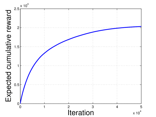
(a)

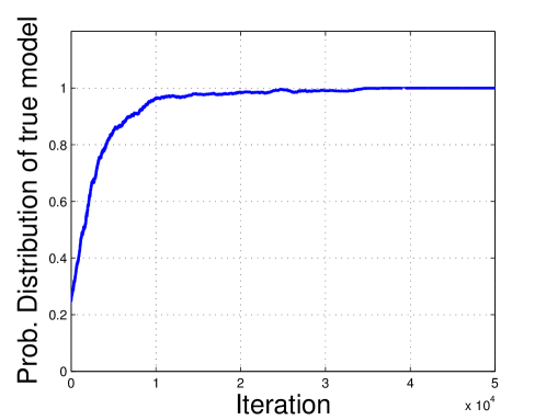
(b)

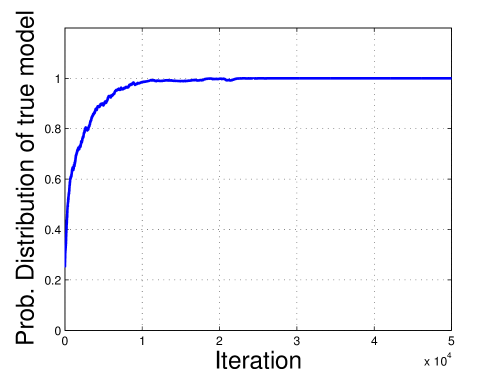
(c)

Figure 6: Expected cumulative regret vs time horizon and probability mass on true model vs time horizon for both type of arms.

We illustrate performance of Thompson sampling algorithm in Fig. 6 for $N=5,$ where $4$ type $A$ items and one type $B$ item. The true model parameters are $p=[0.15,0.25,0.25,0.15,0.15],$ $\rho_{0}=[0.2,0.2,0.1,0.1,0.1],$ and these are assumed unknown. We assume that $\rho_{1}=0.7$ is known. We simulate it with discrete parameter space into a $(2\times 2)$ grid of $(0.15,0.25,0.1,0.2).$ At the start of algorithm, we use uniform prior over the $4$ points for all the arms. We plot the expected cumulative regret as function of time horizon, see Fig. 6-a. The regret incurs whenever sample model different from true model. In Fig. 6-b and Fig. 6-c, we plot the probability distribution on the true model against time for both types of items. We note that probability distribution of true model is approaching to $1,$ in Whittle index based algorithm. This suggests that the Thompson sampling strategy indeed learns the true model rather quickly. A more detailed analysis is being performed.

7 Conclusion

In this paper we studied a restless multi-armed bandit for automated playlist recommendation system with two types of items. We considered infinite horizon discounted and average reward problem. We show that both types arm are indexable and we derived the closed form expression for the Whittle index derived from the state of the belief in the state of the arms and from the model parameters. Our numerical results illustrate that the Whittle index algorithm can perform better than a myopic algorithm. We further discussed the dual speed restless bandit with hidden states and derived Whittle index expression for a variant. We have proposed a Thompson sampling based learning algorithm to learn the true model parameters. Simulation results indicate that the learning is indeed effective. The performance guarantees of the learning algorithm are being investigated.

Appendix 0.A Appendix

0.A.1 Proof of Lemma 2

The proof is similar for type A and type B arm. It has minor variations due to value function expressions. Here, we present the proof for type A arm. We omit the proof for type B arm. The proof is using induction techniques.

1. Let

   $$V_{\beta,1}(\pi,\lambda) = \max\{\lambda,\pi\rho_{0}+(1-\pi)\rho_{1}\}$$

   $$V_{\beta,n+1}(\pi,\lambda) = \max\left\{\lambda+\beta V_{\beta,n}((1-p)\pi,\lambda),\right.$$

   $$\left.\pi\rho_{0}+(1-\pi)\rho_{1}+\beta V_{\beta,n}(1,\lambda)\right\}$$

   The partial derivative of $V_{\beta,1}(\pi,\lambda)$ w.r.t. $\pi$ is $0$ or $-(\rho_{1}-\rho_{0}),$ depending on $\pi,$ and $\lambda.$ Thus the absolute value of slope of $V_{\beta,1}(\pi,\lambda)$ w.r.t. $\pi$ is bounded above by $(\rho_{1}-\rho_{0}).$ Making the induction hypothesis that the absolute value of slope of $V_{\beta,n}(\pi,\lambda)$ w.r.t. $\pi$ is bounded above by $(\rho_{1}-\rho_{0}).$ We next want to show that the absolute value of slope of $V_{\beta,n+1}(\pi,\lambda)$ w.r.t. $\pi$ is bounded above by $(\rho_{1}-\rho_{0}).$

   Note that derivative of the term $\lambda+\beta V_{\beta,n}((1-p)\pi,\lambda)$ w.r.t. $\pi$ is bounded by $(\rho_{0}-\rho_{1})$ because first term is constant and second term’s derivative is bounded by $\beta(1-p)(\rho_{0}-\rho_{1}),$ this is bounded by $(\rho_{1}-\rho_{0}).$

   Also, the absolute value of slope of $\pi\rho_{0}+(1-\pi)\rho_{1}+\beta V_{\beta,n}(1,\lambda)$ w.r.t. $\pi$ is bounded $(\rho_{1}-\rho_{0})$ because first term’s slope is $(\rho_{0}-\rho_{1})$ and second term is constant. Hence the absolute value of slope of $V_{\beta,n+1}(\pi,\lambda)$ w.r.t. $\pi$ is bounded above by $(\rho_{1}-\rho_{0}).$

   By induction, it is true for all $n\geq 1.$ From [4, Chapter $7$], [5, Proposition $2.1,$ Chapter $2$], $V_{\beta,n}(\pi,\lambda)\to V_{\beta}(\pi,\lambda),$ uniformly. Thus the absolute value of slope of $V_{\beta}(\pi,\lambda)$ w.r.t. $\pi$ is bounded above by $(\rho_{1}-\rho_{0}).$

2. The partial derivative of $V_{\beta,1}(\pi,\lambda)$ in (LABEL:algo:iterAlgo_diff) w.r.t. $\lambda$ is $1$ or $0,$ depending on $\pi,$ and $\lambda.$ Thus $\frac{\partial V_{\beta,1}(\pi,\lambda)}{\partial\lambda}<\frac{1}{1-\beta}$ for $0<\beta<1.$ By induction hypothesis $\frac{\partial V_{\beta,n}(\pi,\lambda)}{\partial\lambda}<\frac{1}{1-\beta}.$ The partial derivative of first term in (LABEL:algo:iterAlgo_diff) w.r.t. $\lambda$ is

   $$1+\beta\frac{\partial V_{\beta,n}((1-p)\pi,\lambda)}{\partial\lambda}.$$

   It is bounded above by $\frac{1}{1-\beta}$ by our assumption. The partial derivative of second term in (LABEL:algo:iterAlgo_diff) w.r.t. $\lambda$ is

   $$\beta\frac{\partial V_{\beta,n}(1,\lambda)}{\partial\lambda}$$

   It is also bounded above by $\frac{1}{1-\beta}.$ Hence the partial derivative of $V_{\beta,n+1}(\pi,\lambda)$ w.r.t. $\lambda$ is bounded above by $\frac{1}{1-\beta}.$ By induction, it is true for all $n\geq 1.$ Using earlier technique, $V_{\beta,n}(\pi,\lambda)\to V_{\beta}(\pi,\lambda),$ uniformly. Therefore, $\frac{\partial V_{\beta}(\pi,\lambda)}{\partial\lambda}<\frac{1}{1-\beta}.$

This completes the proof. ∎

0.A.2 Proof of Lemma 3

The proof is analogous for both type A and type B arm. Also, it lead to same Lipschitz constant. Here, we detail the proof for only type A arm and omit it for type B arm.

Fix $\lambda,\beta.$ Define

$$d_{\lambda}(\pi):=V_{1,\beta}(\pi,\lambda)-V_{0,\beta}(\pi,\lambda)$$

We have to show that $d_{\lambda}(\pi_{1})>d_{\lambda}(\pi_{2})$ whenever $\pi_{2}>\pi_{1},$ for all $\pi_{1},\pi_{2}\in[0,1].$ Now

$$d_{\lambda}(\pi_{2})-d_{\lambda}(\pi_{1})=\beta\left(V_{\beta}((1-p)\pi_{1},\lambda)-V_{\beta}((1-p)\pi_{2},\lambda)\right)-(\rho_{1}-\rho_{0})(\pi_{2}-\pi_{1}).$$

From Lemma 2-$1$, we obtain

$$V_{\beta}((1-p)\pi_{1},\lambda)-V_{\beta}((1-p)\pi_{2},\lambda)<(1-p)(\rho_{1}-\rho_{0})|\pi_{1}-\pi_{2}|.$$

Moreover,

$$\beta(1-p)(\rho_{1}-\rho_{0})|\pi_{1}-\pi_{2}|<(\rho_{1}-\rho_{0})|\pi_{1}-\pi_{2}|.$$

This implies $d_{\lambda}(\pi_{2})-d_{\lambda}(\pi_{1})<0$ and our claim follows. ∎

0.A.3 Proof of Lemma 4

• Type A arm:

  Fix $\pi,\beta.$ It is enough to show that $\frac{\partial d_{\lambda}(\pi)}{\partial\lambda}=\frac{\partial V_{1,\beta}(\pi,\lambda)}{\partial\lambda}-\frac{\partial V_{0,\beta}(\pi,\lambda)}{\partial\lambda}<0.$ From equation (LABEL:eq:value-fun-type-a), taking partial derivative w.r.t. $\lambda,$ we obtain

  $$\frac{\partial V_{1,\beta}(\pi,\lambda)}{\partial\lambda} = \beta\frac{\partial V_{0,\beta}(1,\lambda)}{\partial\lambda},$$

  $$\frac{\partial V_{0,\beta}(\pi,\lambda)}{\partial\lambda} = \frac{1-\beta^{K(\pi,\pi_{T})}}{1-\beta}+\beta^{(K(\pi,\pi_{T})+1)}\frac{\partial V_{0,\beta}(1,\lambda)}{\partial\lambda}.$$

  Then

  $$\frac{\partial V_{1,\beta}(\pi,\lambda)}{\partial\lambda}-\frac{\partial V_{0,\beta}(\pi,\lambda)}{\partial\lambda} = \beta\frac{\partial V_{0,\beta}(1,\lambda)}{\partial\lambda}(1-\beta^{K(\pi,\pi_{T})})-\frac{(1-\beta^{K(\pi,\pi_{T})})}{(1-\beta)}.$$

  Rewriting, we have

  $$\frac{\partial d_{\lambda}(\pi)}{\partial\lambda} = (1-\beta^{K(\pi,\pi_{T})})\left[\beta\frac{\partial V_{0,\beta}(1,\lambda)}{\partial\lambda}-\frac{1}{(1-\beta)}\right].$$

  From (LABEL:eq:value-fun-type-a), we can obtain

  $$\frac{\partial V_{0,\beta}(\pi,\lambda)}{\partial\lambda}=\frac{(1-\beta^{\widetilde{K}})}{(1-\beta^{\widetilde{K}+1})(1-\beta)},$$

  where $\widetilde{K}=K(1,\pi_{T}).$ After substitution and simplifying expressions, we have

  $$\frac{\partial d_{\lambda}(\pi)}{\partial\lambda}=\frac{(1-\beta^{K(\pi,\pi_{T})})}{(1-\beta)}\frac{\left(\beta-\beta^{\widetilde{K}+1}-1+\beta^{\widetilde{K}+1}\right)}{(1-\beta^{\widetilde{K}+1})}.$$

  Clearly, $\frac{\partial d_{\lambda}(\pi)}{\partial\lambda}<0$ for $\beta\in[0,1).$

• Type B arm:

  From (7), when $\pi_{T}\in(0,1]$ and all $\pi\in[0,1]$ we can obtain following

  $$\frac{\partial V_{1,\beta}(\pi,\lambda)}{\partial\lambda} = 0,$$

  $$\frac{\partial V_{0,\beta}(\pi,\lambda)}{\partial\lambda} = \begin{cases}1&\mbox{if $T(\pi)<\pi_{T},$}\\ \frac{1}{1-\beta}&\mbox{if $T(\pi)\geq\pi_{T}.$}\end{cases}$$

  Clearly, we have $\frac{\partial d_{\eta}(\pi)}{\partial\eta}<0$ for $\pi_{T}\in(0,1].$ When $\pi_{T}=0,$ we can get

  $$\frac{\partial V_{1,\beta}(\pi,\lambda)}{\partial\lambda} = \frac{\beta}{1-\beta},$$

  $$\frac{\partial V_{0,\beta}(\pi,\lambda)}{\partial\lambda} = \frac{1}{1-\beta}.$$

  Hence $\frac{\partial d_{\lambda}(\pi)}{\partial\lambda}<0.$

This completes the proof. ∎

References

- Agrawal and Goyal [2012] S. Agrawal and N. Goyal. Analysis of Thompson sampling for the multi-armed bandit problem. JMLR Workshop and Conf. Proc., 23:39.1–39.26, 2012.
- Auer et al. [2002] P. Auer, N. Cesa-Bianchi, and P. Fischer. Finite-time analysis of the multiarmed bandit problem. Machine Learning, 47(2-3):235–256, 2002.
- Avrachenkov and Borkar [2015] K. Avrachenkov and V. S. Borkar. Whittle index policy for crawling ephemeral content. Technical Report Report No. 8702, INRIA, 2015. URL https://hal.archives-ouvertes.fr/.
- Bertsekas [1995a] D. P. Bertsekas. Dynamic Programming and Optimal Control, volume 1. Athena Scientific, Belmont, Massachusetts, 1st edition, 1995a.
- Bertsekas [1995b] D. P. Bertsekas. Dynamic Programming and Optimal Control, volume 2. Athena Scientific, Belmont, Massachusetts, 1st edition, 1995b.
- Bubeck and Bianchi [2012] S. Bubeck and N. C. Bianchi. Regret analysis of stochastic and non-stochastic multi-armed bandit problem. Foundations and Trends in Machine Learning, 5(1):1–122, 2012.
- Candes and Tao [2010] E. Candes and T. Tao. The power of convex relaxation: Near optimal matrix completion. IEEE Transactions on Information Theory, 56(5):2053–2080, May 2010.
- Caron et al. [2012] S. Caron, B. Kveton, M. Lelarge, and S. Bhagat. Leveraging side observations in stochastic bandits. Arxiv, 2012.
- Chapelle and Li [2011] O. Chapelle and L. Li. An empirical evaluation of Thompson sampling. In Proc. NIPS, 2011.
- Gittins et al. [2011] J. Gittins, K. Glazebrook, and R. Weber. Multi-armed Bandit Allocation Indices. John Wiley and Sons, New York, 2nd edition, 2011.
- Gopalan and Mannor [2015] A. Gopalan and S. Mannor. Thompson sampling for learning parameterized Markov decision processes. In Proc. COLT, 2015.
- Gopalan et al. [2014] A. Gopalan, S. Mannor, and Y. Mansour. Thompson sampling for complex online problems. In Proc. ICML, 2014.
- Hariri et al. [2012] N. Hariri, B. Mobasher, and R. Burke. Context-aware music recommendation based on latent topic sequential patterns. In Proc. ACM RecSys, 2012.
- Lai and Robbins [1985] T. L. Lai and H. Robbins. Asymptotically efficient adaptive allocation rules. Advances in Applied Mathematics, 6(1):4–22, March 1985.
- Langford and Zhang [2007] J. Langford and T. Zhang. The epoch-greedy algorithm for contextual multi-armed bandits. In Proc. NIPS, 2007.
- Li et al. [2010] L. Li, W. Chu, J. Langford, and R. E. Schapire. A contextual-bandit approach to personalized news article recommendation. In Proc. ACM WWW, 2010.
- Liu et al. [2013] H. Liu, K. Liu, and Q. Zhao. Learning in a changing world: Restless multiarmed bandit with unknown dynamics. IEEE Transactions on Information Theory, 59(3):1902–1916, March 2013.
- Liu and Zhao [2010] K. Liu and Q. Zhao. Indexability of restless bandit problems and optimality of Whittle index for dynamic multichannel access. IEEE Transactions Information Theory, 56(11):5557–5567, November 2010.
- Meshram et al. [2015] R. Meshram, D. Manjunath, and A. Gopalan. A restless bandit with no observable states for recommendation systems and communication link scheduling. In Proc. IEEE CDC, 2015.
- Meshram et al. [2016a] R. Meshram, A. Gopalan, and D. Manjunath. Optimal recommendation to users that react: Online learning for a class of POMDPs. In Proc. IEEE CDC, 2016a.
- Meshram et al. [2016b] R. Meshram, A. Gopalan, and D. Manjunath. Optimal recommendation to users that react: Online learning for a class of POMDPs. Arxiv, 2016b.
- Meshram et al. [2016c] R. Meshram, D. Manjunath, and A. Gopalan. On the Whittle index for restless multi-armed hidden markov bandits. Arxiv, 2016c.
- Meshram et al. [2017] R. Meshram, A. Gopalan, and D. Manjunath. Restless bandits that hide their hand and recommendation systems. In Proc. IEEE COMSNETS, 2017.
- Papadimitriou and Tsitsiklis [1999] C. H. Papadimitriou and J. H. Tsitsiklis. The complexity of optimal queueing network control. Mathematics of Operations Research, 24(2):293–305, May 1999.
- Ross [1971] S. M. Ross. Quality control under Markovian deterioration. Management Science, 17(9):587–596, May 1971.
- Ross [1993] S. M. Ross. Applied Probability Models with Optimization Applications. Dover Publications, 1993.
- Thompson [1933] W. R. Thompson. On the likelihood that one unknown probability exceeds another in view of the evidence of two samples. Biometrika, 24(3–4):285–294, 1933.
- Walter [1976] R. Walter. Principles of Mathematical Analysis. McGraw-Hill Book Co., Third edition, 1976.
- Whittle [1988] P. Whittle. Restless bandits: Activity allocation in a changing world. Journal of Applied Probability, 25(A):287–298, 1988.