Quantum sensors for the generating functional of interacting quantum field theories

Abstract

Difficult problems described in terms of interacting quantum fields evolving in real time or out of equilibrium are abound in condensed-matter and high-energy physics. Addressing such problems via controlled experiments in atomic, molecular, and optical physics would be a breakthrough in the field of quantum simulations. In this work, we present a quantum-sensing protocol to measure the generating functional of an interacting quantum field theory and, with it, all the relevant information about its in or out of equilibrium phenomena. Our protocol can be understood as a collective interferometric scheme based on a generalization of the notion of Schwinger sources in quantum field theories, which make it possible to probe the generating functional. We show that our scheme can be realized in crystals of trapped ions acting as analog quantum simulators of self-interacting scalar quantum field theories.

I Introduction

Some of the most complicated problems of theoretical physics arise in the study of quantum systems with a large, sometimes even infinite, number of coupled degrees of freedom. These complex problems arise in our effort to understand certain observations in condensed-matter cm_book or high-energy physics qft_book , which one tries to model with the unifying language of quantum field theories (QFTs). More recently, the field of atomic, molecular and optical (AMO) physics is providing experimental setups QS_cold_atoms ; QS_trapped_ions that aim at targeting similar problems. The approach is, however, rather different. These AMO setups can be microscopically designed to behave with great accuracy according to a particular model of interest. Hence, it is envisioned that one will be capable of answering open questions about a many-body model described through a QFT by preparing, evolving, and measuring the experimental system; what has been called a quantum simulation feynman_qs ; qs_goals .

Either in the form of piecewise time evolution by concatenated unitaries digital_QS , i.e. digital quantum simulation (DQS), or continuous time evolution by always-on couplings analog_QS , i.e. analog quantum simulation (AQS), the main focus in this field has been typically placed on the quantum simulation of condensed-matter problems QS_cold_atoms ; QS_trapped_ions ; qs_book . Nonetheless, some theoretical works have also addressed how quantum simulators could mimic the relativistic QFTs that appear in high-energy physics, as occurs for the AQS of a Klein-Gordon QFT with Bose-Einstein condensates aqs_qft_bosons_bec ; aqs_qft_bosons_bec_detection . Note, however, that the most versatile AMO quantum simulators to date QS_cold_atoms ; QS_trapped_ions do not work directly in the continuum, but on a physical lattice that is either provided by additional laser dipole forces for neutral atoms QS_cold_atoms , or by the interplay of Coulomb repulsion and electromagnetic oscillating forces for singly-ionized atoms QS_trapped_ions . Therefore, the relevant symmetries of the high-energy QFT, such as Lorentz invariance, must emerge as one takes the continuum/low-energy limit in the AMO quantum simulator. This occurs trivially for free fermionic QFTs comment_free_fermions , which underlies the schemes for the AQS of Dirac QFTs with ultra-cold atoms in optical lattices aqs_qft_fermions . There are also proposals for interacting QFTs, such as the DQS of self-interacting Klein-Gordon fields dqs_qft_phi4 , the analog aqs_qft_boson_fermion and digital dqs_qft_boson_fermion quantum simulators of coupled Fermi-Bose fields, and an ultra-cold atom AQS of Dirac fields with self-interactions or coupled to scalar bosonic fields aqs_qft_fermions_interactions .

In the interacting case, as discussed in aqs_qft_fermions_interactions ; dqs_qft_phi4 , renormalization techniques must be employed to set the right bare parameters in such a way that a QFT with the required Lorentz symmetry and free of ultraviolet (UV) divergences is obtained in the continuum limit. This is the standard situation in lattice field theories book_lattice , where the continuum limit is obtained by letting the lattice spacing $a\to 0$, removing thus the natural UV cut-off of the lattice, while maintaining a finite renormalized mass/gap $m$ describing the physical mass of the particles in the corresponding QFT. This requires setting the bare parameters close to a critical point of the lattice model, where the dimensionless correlation length, measured in lattice units, diverges $\tilde{\xi}\to\infty$. In this case, the mass $m\sim 1/\tilde{\xi}a$ can remain constant even for vanishingly small lattice spacings. Therefore, the experience gained in the classical numerical simulation of interacting QFTs on the lattice will be of the utmost importance for the progress of quantum simulators of high-energy physics problems.

In a more direct connection to open problems in high-energy physics, e.g. the phase diagram of quantum chromodynamics qcd_phase_diagram , we note that there has been a number of proposals for the DQS dqs_lattice_gauge_theories ; dqs_qft_gauge_U(1)_qlinks ; dqs_lattice_gauge_theories ; dqs_qft_SU(2)_qlinks and AQS aqs_qft_gauge_U(1)_qlinks ; aqs_QED ; aqs_qft_gauge_U(1)_qlinks ; aqs_qft_fermions_U(1)_qlinks ; aqs_qft_fermions_SU(2)_qlinks ; aqs_qft_fermions_U(1)_qlinks ; aqs_qft_fermions_SU(2)_qlinks of gauge theories. As announced above, previous knowledge from lattice gauge theories has been essential to come up with schemes for the quantum simulation of Abelian aqs_qft_gauge_U(1)_qlinks ; dqs_qft_gauge_U(1)_qlinks and non-Abelian dqs_qft_SU(2)_qlinks QFTs of the gauge sector, as well as Abelian aqs_QED ; aqs_qft_fermions_U(1)_qlinks and non-Abelian aqs_qft_fermions_SU(2)_qlinks QFTs of gauge fields coupled to Dirac fields. Starting from the simpler QFTs discussed above, this body of work constitutes a well-defined long-term roadmap for the implementation of relevant models of high-energy physics in AMO platforms zohar_review . In this work, we address the question of devising a general measurement strategy to extract the properties of an interacting QFT, which could be adapted to these different quantum simulators. One possibility would be to mimic the high-energy scattering experiments in particle accelerators by preparing wave packets and measuring the outcome after a collision, as proposed in the context of DQS dqs_qft_phi4 . In this work, we explore a different possibility that would allow the quantum simulator to extract the complete information about an interacting QFT. We introduce a scheme that is capable of measuring the generating functional of the QFT qft_book . In particular, this functional can be used to extract the Feynman propagator, such that one can also make predictions about different scattering experiments. In addition, other relevant properties of the interacting QFT can also be directly extracted from such a functional. Moreover, our scheme is devised for analog quantum simulators, such that the resource requirements are lower than those of a DQS using a fault-tolerant quantum computing hardware.

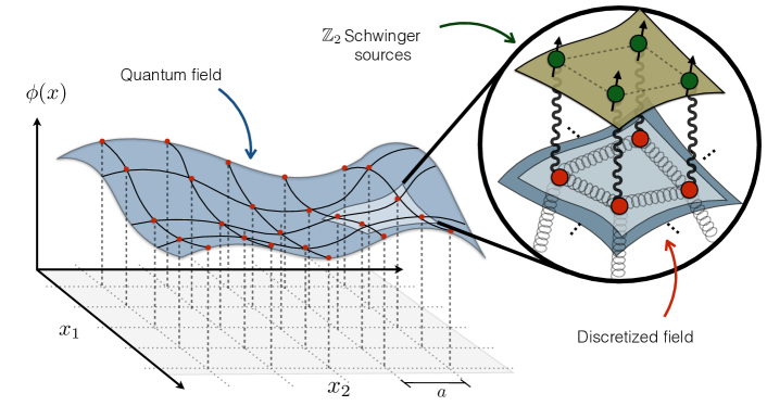
Figure 1: Schematic representation of the Schwinger sensors for the generating functional: We represent a quantum scalar field $\phi(x)$ in a $D=2+1$ space-time, which is discretized into a $d=2$ spatial lattice, while letting the time coordinate continuous. (inset) Zoom of a small space region, where the field at each point (red circles) is coupled to the fields at neighbouring points (small springs), and can be excited by its coupling (wavy lines) to generalised quantum-mechanical Schwinger sources (green circles with arrows). These $\mathbb{Z}_{2}$ Schwinger sources will also function as quantum sensors for the generating functional.

II Sensors for quantum field theories (QFTs)

In this section, we introduce a scheme to measure the generating functional of a QFT directly in the continuum. For the sake of concreteness, we present our results by focusing on a real scalar QFT, and comment on generalizations to other QFTs at the end of the section.

II.1 Self-interacting Klein-Gordon QFT, Schwinger sources, and the generating functional

Let us consider a self-interacting real Klein-Gordon QFT, which is described by the bosonic scalar field operator $\phi(x)$, where $x=(t,\bf{x})$ is a point in the $D=(d+1)$-dimensional Minkowski space-time with coordinates $x^{\mu}$, $\mu\in\{0,\cdots,d\}$, and we set $\hbar=c=k_{\rm B}=1$. The Lagrangian density that governs the dynamics of the scalar field is

$$\mathcal{L}=\frac{1}{2}\partial_{\mu}\phi(x)\partial^{\mu}\phi(x)-\frac{m_{0}^{2}}{2}\phi(x)^{2}-\mathcal{V}(\phi),$$ (1)

where $\partial_{\mu}=\partial/\partial x^{\mu}$, $\partial^{\mu}=\eta^{\mu\nu}\partial_{\nu}$ with Minkowski’s metric $\eta={\rm diag}(1,-1,\cdots,-1)$, and we use Einstein’s summation criterion for repeated indexes. Here, $m_{0}$ is the bare mass of the scalar boson, and $\mathcal{V}(\phi)$ describes its self-interaction through non-linearities e.g. $\lambda\phi^{4}$ or $\cos(\beta\phi)$. In these units, in order to make the action $S=\int{\rm d}^{D}x\mathcal{L}$ dimensionless, the scalar field must have classical mass dimensions $d_{\phi}=(D-2)/2$, while the couplings have $d_{m_{0}^{2}}=2$ and $d_{\lambda}=(4-D)$.

Let us now introduce the so-called Schwinger sources schwinger , which are classical background fields that generate excitations of the quantum field. For the real scalar QFT qft_book , it suffices to introduce a classical scalar background field $J(x)$ and modify the Lagrangian according to

$$\mathcal{L}\to\mathcal{L}_{J}=\mathcal{L}+J(x)\phi(x),$$ (2)

where the sources have mass dimension $d_{J}=(D+2)/2$. The normalized generating functional is obtained from the vacuum-to-vacuum propagator, after removing processes where particles are spontaneously created/annihilated in the absence of the Schwinger sources. This can be expressed as

$$\mathsf{Z}[J(x)]=\bra{\Omega}\mathsf{T}\!\left\{{\rm e}^{{\rm i}\int{\rm d}^{D}xJ(x)\phi_{H}(x)}\right\}\ket{\Omega},$$ (3)

where we have introduced the ground state of the interacting QFT $\ket{\Omega}$, and used the time-ordering symbol $\mathsf{T}$. Additionally, the field operators are expressed in the Heisenberg picture of the interacting QFT in the absence of Schwinger sources. This is achieved by defining $\phi_{H}(x)=\mathsf{T}\{{\rm e}^{{\rm i}\int{\rm d}^{D}x\mathcal{H}}\}\phi(x)\mathsf{T}\{{\rm e}^{-{\rm i}\int{\rm d}^{D}x\mathcal{H}}\}$, where the integral in the evolution operator includes integration over time, and

$$\mathcal{H}=\frac{1}{2}\pi(x)^{2}+\frac{1}{2}\bm{\nabla}\phi(x)^{2}+\frac{m_{0}^{2}}{2}\phi(x)^{2}+\mathcal{V}(\phi)$$ (4)

is the Hamiltonian density associated to the QFT under study (1). Here, $\pi(x)=\partial_{t}\phi(x)$ is the conjugate momentum fulfilling the equal-time canonical commutation relations with the scalar field $[\phi(t,{\bf x}),\pi(t,{\bf y})]={\rm i}\delta^{d}({\bf x}-{\bf y})$.

The normalized generating functional, hereafter simply referred to as the generating functional, contains all the relevant information about the QFT. In particular, any $n$-point Feynman propagator $G^{(n)}=\bra{\Omega}\mathsf{T}\left\{\phi_{H}(x_{1})\cdots\phi_{H}(x_{n})\right\}\ket{\Omega}$ can be obtained from $\mathsf{Z}[J]$ by functional differentiation

$$G^{(n)}(x_{1},\cdots,x_{n})=(-{\rm i})^{n}\left.\frac{\delta^{n}\mathsf{Z}[J(x)]}{\delta J(x_{1})\cdots\delta J(x_{n})}\right|_{J=0}.$$ (5)

Note that we are using the normalized generating functional (3), such that the factor $\mathsf{Z}^{-1}(0)$ in the propagator (5) disappears as $\mathsf{Z}(0)=1$. Through the Gell-Mann-Low theorem gellman_low , one can express the generating functional, and thus any $n$-point propagator of the interacting QFT, in terms of Feynman diagrams. Accordingly, $\mathsf{Z}[J]$ becomes a fundamental tool in the theoretical study of interacting QFTs. The question that we address in the following subsection is if such a functional can also become an observable in some experiment. Note that we are not referring to susceptibilities expressed in terms of retarded Green’s functions, which are typically measured in linear-response experiments. We are instead looking for a scheme that allows one to measure the complete generating functional, out of which one could calculate any time-resolved Feynman propagator, or obtain predictions of any type of scattering experiment. The generating functional does indeed contain all the relevant information about a QFT.

II.2 $\mathbb{Z}_{2}$ Schwinger sources

The proposed scheme promotes the classical Schwinger fields (2) to quantum-mechanical $\mathbb{Z}_{2}$ Schwinger sources. In particular, we will consider the $\mathfrak{su}(2)$ Lie algebra, and define the operators $\sigma^{\alpha}$, where $\sigma^{0}=\mathbb{I}$, and $\{\sigma^{\beta}\}_{\beta=1,2,3}$ are the well-known Pauli matrices. The $\mathbb{Z}_{2}$ Schwinger field now reads

$$J(x)\to\sum_{\alpha}J^{\alpha}(x)\sigma^{\alpha}(x),$$ (6)

where $J^{\alpha}(x)$ are classical background fields, and $\sigma^{\alpha}(x)$ can be interpreted as the operators of an ancillary two-level system (i.e. spin-1/2, qubit) that is attached to every space-time coordinate. We advance, however, that for AQS of QFTs on the lattice, we shall not need a continuum but a countable set of ancillary spins/qubits (see Fig. 1).

The classical background field (2), which was introduced by Schwinger as a mathematical artefact in order to calculate the generating functional of the interacting QFT (3), has now been promoted onto a quantum-mechanical source that may also have its own dynamics described by a generic Hamiltonian $\mathcal{H}_{\sigma}$. Hence, Eq. (4) must be substituted by

$$\mathcal{H}\to\mathcal{H}_{J}=\mathcal{H}+\mathcal{H}_{\sigma}-\sum_{\alpha}J^{\alpha}(x)\sigma^{\alpha}(x)\phi(x).$$ (7)

The main idea is that these quantum sources will not only act as generators of excitations in the quantum field, but also as quantum probes capable of measuring the generating functional of the interacting QFT. We discuss below a particular measurement protocol to achieve this goal.

The use of quantum-mechanical two-level systems as sensors for measuring physical quantities with high precision, such as electric/magnetic fields or oscillator frequencies, is a well-developed technique in AMO physics q_sensors_review . In the two most standard cases, the two-level system can get excited (i.e. Rabi probe) or gain a relative phase (i.e. Ramsey probe) as a consequence of its coupling to the physical quantities that need to be measured. In many situations of experimental relevance, one uses a single quantum sensor, and maintains its quantum coherence for ever-increasing periods of time to improve the sensitivity of the measurement apparatus. In the context of QFTs, ever since the pioneering work of W. G. Unruh unruh_detector , Rabi-type probes based on a single particle with discrete energy levels have been routinely considered as detectors of quantum fields book_cureved_qft . These type of detectors have also been considered in a quantum-simulation context aqs_qft_bosons_bec_detection ; aqs_qft_effects_ions . In contrast, Ramsey-type probes have been mainly considered for the quantum simulation of condensed-matter problems (see e.g. aqd_bec ). On the other hand, in the context of high-energy physics, Ramsey probes remain largely unexplored (an exception is Ref. zohar_ramsey , which discusses interferometric measurements of string tension and the Wilson-loop operator in gauge theories). In this work, we partially fill this gap by showing that the interacting relativistic QFT (7) with $\mathfrak{su}(2)$ Schwinger sources of the Ramsey type, i.e. setting $J^{\alpha}(x)=J(x)(\delta_{\alpha,0}-\delta_{\alpha,3})/2$, can function as a quantum sensor for the QFT generating functional. This particular choice of the generalised Schwinger sources guarantees a differential coupling of the field to the internal states of the sensors, such that their relative phase will depend on the time-evolution of the quantum scalar field. In the following we will show that a collective interferometric scheme can exploit this differential coupling to probe the full generating functional.

II.3 Quantum sensors for the generating functional

In addition to exploiting the quantization of energy levels and the quantum coherence, quantum sensors based on ensembles of two-level systems can make use of entanglement to increase their sensitivity entanglement_metrology , or to gain information about equal-time density-density correlations from their short-time dynamics density_correlations , which can be of interest in the quantum simulation of condensed-matter problems. In our case, entanglement is not used to increase the sensitivity, but is also an ingredient of paramount importance to map the whole information of the relativistic QFT, which is encoded in the generating functional $\mathsf{Z}[J]$, into the ensemble of $\mathbb{Z}_{2}$ Schwinger sources/sensors. Let us describe in detail the protocol.

We consider an initial state in the remote past as the tensor product of the interacting QFT ground state $\ket{\Omega}$ and the quantum sensor state with all spins pointing down $\ket{0_{\sigma}}$. This assumes that the state of the quantum field is adiabatically prepared in the remote past by starting from the non-interacting ground state, and switching on the self-interactions $V(\phi)$ sufficiently slow, i.e. adiabatically, while the Schwinger-source couplings remain switched off. One then applies a fully entangling operation to the sensors generating the so-called Greenberger-Horne-Zeilinger (GHZ) states ghz , which are multi-partite generalizations of the Einstein-Podolski-Rosen (EPR) states epr . This leads to

$$\ket{\Psi(t_{0})}=\ket{\Omega}\otimes\frac{1}{\sqrt{2}}\left(\prod_{{\bf x}}\sigma^{0}(t_{0},{\bf x})+\prod_{{\bf x}}\sigma^{1}(t_{0},{\bf x})\right)\ket{0_{\sigma}}.$$ (8)

At this instant of time $t_{0}$, the Schwinger-source couplings are switched on. The time-evolution operator of the full sourced QFT (7) can be expressed in the interaction picture with respect to $\mathcal{H}_{0}(x)=\mathcal{H}+\mathcal{H}_{\sigma}$, being $\mathcal{H}$ the Hamiltonian of the sourceless interacting QFT (4). In the distant future, the time-evolution operator becomes

$$U_{J}=\mathsf{T}\left\{{\rm e}^{-{\rm i}\int{\rm d}^{D}x\mathcal{H}_{0}(x)}\right\}\mathsf{T}\left\{{\rm e}^{+{\rm i}\int{\rm d}^{D}xJ(x)\phi_{\rm H}(x)P_{\rm H}(x)}\right\},$$ (9)

where $P_{\rm H}(x)=\mathsf{T}\{{\rm e}^{{\rm i}\int{\rm d}^{D}x\mathsf{H}_{\sigma}(x)}\}P(t_{0},{\bf x})\mathsf{T}\{{\rm e}^{-{\rm i}\int{\rm d}^{D}x\mathcal{H}_{\sigma}(x)}\}$, and $P(t_{0},{\bf x})=\textstyle\frac{1}{2}(\sigma^{0}({\bf x})-\sigma^{3}({\bf x}))$ is an orthogonal projector onto the ground state of the $\mathbb{Z}_{2}$ sensor localized at coordinate $(t_{0},\bf{x})$. Finally, the observable information about the generating functional will be encoded in the expectation value of a spin parity operator

$$\mathsf{P}[J(x)]=\bra{\Psi(t_{0})}U_{J}^{\dagger}\prod_{{\bf x}}\sigma^{1}(t_{0},{\bf x})U_{J}\ket{\Psi(t_{0})}.$$ (10)

We will consider a simple Hamiltonian for the quantum sensors

$$\mathcal{H}_{\sigma}=\delta\epsilon(\sigma^{0}(t_{0},{\bf x})-P(t_{0},{\bf x})),$$ (11)

where $\delta\epsilon$ is the energy-density associated to the transition frequency $\omega_{0}$ between the two levels of the sensor, which has a natural realization in quantum-simulation AMO platforms. For this particular choice, one finds that the expectation value of the parity operator evolves according to $\mathsf{P}[J]=\bra{\Omega}\mathsf{T}\left\{{\rm e}^{{\rm i}\int{\rm d}^{D}x(\delta\epsilon+J(x)\phi_{\rm H}(x))}\right\}\ket{\Omega}+{\rm c.c.}$, and thus encodes the generating functional (3), namely

$$\mathsf{P}[J(x)]=\textstyle\frac{1}{2}{\rm e}^{{\rm i}\int{\rm d}^{D}x\delta\epsilon}\mathsf{Z}[J(x)]+{\rm c.c.}$$ (12)

Let us recapitulate the results obtained so far. By introducing a quantum sensor $\sigma^{\alpha}(x)$ at each space-time coordinate, thus upgrading the standard Schwinger sources to $\mathbb{Z}_{2}$ fields (6), we have constructed a parity Ramsey interferometer capable of encoding the generating functional of an interacting QFT in its time-evolution (12) for a particular set of background sources fulfilling $J^{\alpha}(x)=J(x)(\delta_{\alpha,0}-\delta_{\alpha,3})/2$.

II.4 Simplified sensors for Feynman propagators

In this section, we show that the protocol can be simplified considerably if one is only interested in $n$-point Feynman propagators (5). Such propagators contain a lot of information relevant to the typical scattering experiments and other types of real-time non-equilibrium phenomena. For even $n$, these Feynman propagators can be inferred from the Ramsey parity signal by functional differentiation

$$\left.\frac{\delta^{n}\mathsf{P}[J(x)]}{\delta J(x_{1})\cdots\delta J(x_{n})}\right|_{J=0}=\textstyle\frac{1}{2}{\rm e}^{{\rm i}\int{\rm d}^{D}x\delta\epsilon}G^{(n)}(x_{1},\cdots,x_{n})+{\rm c.c.},$$ (13)

where we have assumed that an approximate remote-past to distant-future time-evolution is obtained by setting $t-t_{0}>{\rm max}\{|x_{i}^{0}-x_{j}^{0}|,\hskip 4.30554pt\forall\hskip 2.15277pti,j=1,\cdots,n\}$.

To estimate such functional derivatives, the required Schwinger field $J(x)$ that must be experimentally applied would be a comb of $n$ point-like sources

$$J(x)=\sum_{i=1}^{n}\mathsf{J}_{i}\delta^{D}(x-x_{i}),$$ (14)

where $\mathsf{J}_{i}$ are the strengths of infinitesimal field-sensor couplings at the particular space-time coordinates $x_{i}$. Since the Schwinger field (14) is only applied to a subset of the quantum sensors located at $X_{\rm s}=\{{\bf x}_{1}\cdots{\bf x}_{n}\}$, which already requires addressability, we may also consider that the initial entangling operation may only involve that particular subset. In that case, one can simplify the required initial state (8) to

$$\ket{\Psi(t_{0})}=\ket{\Omega}\otimes\frac{1}{\sqrt{2}}\left(\prod_{{\bf x}\in X_{\rm s}}\sigma^{0}(t_{0},{\bf x})+\prod_{{\bf x}\in X_{\rm s}}\sigma^{1}(t_{0},{\bf x})\right)\ket{0_{\sigma}}.$$ (15)

The fact that a GHZ state of all the spins is no longer required is a very important simplification, and also makes the protocol more robust as one considers the degrading effect of external sources of noise. Additionally, we do not require to measure the full spin parity (10), but only

$$\mathsf{P}[J(x)]=\bra{\Psi(t_{0})}U_{J}^{\dagger}\prod_{{\bf x}\in X_{\rm s}}\sigma^{1}(t_{0},{\bf x})U_{J}\ket{\Psi(t_{0})}.$$ (16)

Note that mobile sensors might be available depending on the particular implementation. In that case, we do not require a quantum sensor at every space-time coordinate, but only $n$ sensors located at the corresponding points $\mathcal{H}_{\sigma}=\sum_{j=1}^{n}\delta\epsilon(\sigma^{0}(t_{0},{\bf x})-P(t_{0},{\bf x}))\delta^{d}({\bf x}-{\bf x}_{j})$.

To infer the value of the functional derivative of the parity signal (16), one needs to apply different sets of instantaneous sources (14), which we label by ${\mathbf{J}}^{(m)}=\left(\mathsf{J}_{1}^{(m)},\cdots,\mathsf{J}_{n}^{(m)}\right)$ with $m=1,\cdots,M$. For each of these sets of sources, one would then measure the corresponding parity oscillations $\mathsf{P}[{\mathbf{J}}^{(m)}]$. Finally, by adding and subtracting these parities according to a given prescription obtained by the discretization of the functional derivatives, one can infer an estimate of the $n$-point Feynman propagators via Eq. (13).

To be more concrete, let us consider the important case of the single-particle 2-point Feynman propagator $\Delta(x_{1}-x_{2})=G^{(2)}(x_{1},x_{2})$. In this case, our protocol requires creating a simple EPR pair between two distant quantum sensors at ${{\bf x}_{1},{\bf x}_{2}}$ (15). Additionally, we have to consider $M=4$ different measurements of the Ramsey parity signal for a time longer than $|x_{1}^{0}-x_{2}^{0}|$ with the following sets of Schwinger sources: ${\mathbf{J}}^{(1)}=(0,0)$, ${\mathbf{J}}^{(2)}=({\mathsf{J}}_{1},0)$, $\bm{{\mathbf{J}}^{(3)}}=({\mathsf{J}}_{1},{\mathsf{J}}_{2})$, and ${\mathbf{J}}^{(4)}=(0,{\mathsf{J}}_{2})$. Using these sets of infinitesimal Schwinger sources, one can reconstruct the discretization of the two functional derivatives required to calculate the single-particle Feynman propagator in Eq. (5) for $n=2$. Therefore, the Feynman propagator can then be inferred from

$$\sum_{m=1}^{4}\frac{(-1)^{m}\mathsf{P}[{\mathbf{J}}^{(m)}]}{{\mathsf{J}}_{1}{\mathsf{J}}_{2}}\approx-{\rm e}^{{\rm i}2\omega_{0}(t-t_{0})}\Delta(x_{1}-x_{2})+{\rm c.c.},$$ (17)

where we have assumed that ${\mathsf{J}}_{1},{\mathsf{J}}_{2}\ll m_{0}^{2}$, and where $m_{0}$ is the bare mass of the QFT (1). According to this expression, we can infer the real (imaginary) part of the propagator by measuring at $\tau=2\pi r/\omega_{0}$ ($\tau=(2r+1)\pi/2\omega_{0}$), where $r\in\mathbb{Z}$.

Let us now advance on the results of the following section, where we discuss an implementation of this sensing scheme using AMO quantum simulators of QFTs. In this case, the quantum sensors can also have spurious couplings to other quantum/classical fields, e.g. environmental electromagnetic fields, which cannot be switched on/off, but instead act continuously during the probing protocol. Accordingly, the parity oscillations will also get damped as a function of the probing time with a characteristic dephasing time $T_{2}$. Assuming that evolution of the field-sensor mixed state can be described in the Markovian regime, which is the case in many AMO platforms, the effects of the noise on the time-evolution amounts to substituting ${\rm e}^{{\rm i}n\omega_{0}(t-t_{0})}\to{\rm e}^{{\rm i}n\omega_{0}(t-t_{0})}{\rm e}^{-\mathfrak{f}(\{x_{j}\})(t-t_{0})/T_{2}}$ in the previous expressions, where $\mathfrak{f}(\{x_{j}\})$ is a particular function of the number and positions of the probes. In some situations, as occurs for the trapped-ion crystals monz_14_qubit_entanglement described below, these spurious couplings are mainly due to global fields, and $f(\{x_{j}\})=(\sum_{j}1)^{2}=n^{2}$, such that the visibility of the Ramsey parity signal decays faster as the number of quantum sensors increases, limiting the advantage of this type of entangled quantum sensors in other contexts entangled_q_Sensors_noise . This sets a constraint into the proposed protocol, as only space-time coordinates fulfilling ${\rm max}\{|x_{i}^{0}-x_{j}^{0}|\}<\tau\ll T_{2}/n^{2}$ could be probed.

To overcome this limitation, and given that the protocol already requires single-probe addressability, one may encode the sensors in a decoherence-free subspace by considering an entangled Neel-type initial state

$$\ket{\Psi_{\pm}(t_{0})}=\ket{\Omega}\otimes\frac{1}{\sqrt{2}}\left(\prod_{{\bf x}\in X_{\rm e}}\sigma^{1}(t_{0},{\bf x})\pm\prod_{{\bf x}\in X_{\rm o}}\sigma^{1}(t_{0},{\bf x})\right)\ket{0_{\sigma}}.$$ (18)

where $X_{\rm o}=\{{\bf x}_{1},{\bf x}_{3}\cdots{\bf x}_{n-1}\}$, and $X_{\rm e}=\{{\bf x}_{2},{\bf x}_{4}\cdots{\bf x}_{n}\}$. Additionally, the Schwinger sources (6) must be modified to $J_{\alpha}(x)=J(x)\delta_{\alpha,3}/2$, and the Schwinger field (14) must become staggered $J(x)=\sum_{i=1}^{n}\mathsf{J}_{i}(-1)^{i+1}\delta^{D}(x-x_{i}),$ which requires alternating field-sensor couplings. In this case, the parity signals for each of the entangled Neel-type initial states $\mathsf{P}_{\pm}[J]=\bra{\Psi_{\pm}(t_{0})}U_{J}^{\dagger}\prod_{{\bf x}\in X_{\rm s}}\sigma^{1}(t_{0},{\bf x})U_{J}\ket{\Psi_{\pm}(t_{0})}$ lead to the following functional derivatives

$$\left.\frac{\delta^{n}\mathsf{P}{{}_{\pm}}[J(x)]}{\delta J(x_{1})\cdots\delta J(x_{n})}\right|_{J=0}=\textstyle\frac{1}{2}G^{(n)}(x_{1},\cdots,x_{n})\pm{\rm c.c.},$$ (19)

which directly yield the real ($+$) and imaginary ($-$) parts of the $n$-point propagator. The prescription to evaluate the functional derivatives would be similar as the one described above. In the ideal case, we have assumed that $f(\{x_{j}\})=(\sum_{j}(-1)^{j})^{2}=0$, such that no decoherence will affect the parity signals. In practice, as discussed in more detail below, there will be non-global components of the source-field coupling and other sources of noise that will degrade the visibility of the parity oscillations, limiting the possible space-time points of the propagators that can be measured. We would also like to comment on a different strategy to combat the effect decoherence by combining the measurement scheme for the propagators (17) with dynamical decoupling techniques (i.e. concatenated spin-echo sequences) dyn_decoupling . In the impulsive regime where the Schwinger sources are switched on/off very fast (14), the spin echoes will only refocus the decohering effect of the much slower fluctuating fields, but will not affect the signal that we aim to measure.

II.5 Finite temperature and other interacting QFTs

So far, we have focused on a self-interacting bosonic QFT at $T=0$. As mentioned in the introduction, the connection to open problems in high-energy physics, such as the phase transition between the hadron gas and quark-gluon plasma in quantum chromodynamics, would require considering finite-$T$ regimes and other QFTs that include fermionic matter at finite densities coupled to gauge fields. The question that we thus address in this subsection is whether the sensing scheme for the generating functional can be applied to finite temperatures, and generalized to other QFTs.

Let us start by discussing the finite-$T$ regime in the self-interacting Klein-Gordon QFT (1). The generating functional in this case becomes

$$\mathsf{Z}_{T}[J(x)]={\rm Tr}\left(\rho_{T}\mathsf{T}\left\{{\rm e}^{{\rm i}\int{\rm d}^{D}xJ(x)\phi_{H}(x)}\right\}\right),$$ (20)

where $\rho_{T}={\rm e}^{-\beta\int{\rm d}^{d}x\mathcal{H}}/{\rm Tr({\rm e}^{-\beta\int{\rm d}^{d}x\mathcal{H}}})$ is the Gibbs state of the QFT with Hamiltonian $\mathcal{H}$ (4) at temperature $T=1/\beta$. By functional differentiation, and using Eq. (5), one recovers the correct $n$-point Feynman propagators at finite temperature $G^{(n)}={\rm Tr}\left(\rho_{T}\mathsf{T}\left\{\phi_{H}(x_{1})\cdots\phi_{H}(x_{n})\right\}\right)$. Such a functional can be inferred from the spin parity oscillations of the quantum sensors, provided that the initial state is $\rho(t_{0})=\rho_{T}\otimes\ket{\Psi(t_{0})}\bra{\Psi(t_{0})}$, where the initial state for the sensors corresponds to the GHZ state of Eq. (8). In this case, we are assuming that the self-interacting Gibbs state $\rho_{T}$ can be prepared dissipatively in the distant past, while the GHZ spin state is prepared in analogy to the $T=0$ case. Since the distant-future time-evolution operator is still given by Eq. (9), one can directly prove that the finite-$T$ spin parity evolves as

$$\mathsf{P}_{T}[J]={\rm Tr}\left(\!\rho(t_{0})U_{J}^{\dagger}\prod_{{\bf x}}\sigma^{1}(t_{0},{\bf x})U_{J}\!\right)=\textstyle\frac{1}{2}{\rm e}^{{\rm i}\int{\rm d}^{D}x\delta\epsilon}\mathsf{Z}_{T}[J]+{\rm c.c.},$$ (21)

and thus encodes the desired finite-$T$ generating functional. From this expression, one can directly reproduce the previous results for the Feynman propagators, which now correspond to finite-$T$ time-ordered Green’s functions. This can be generalized to initial states that are diagonal in the energy eigenbasis of the interacting QFT, but not necessarily distributed according to the Boltzmann weights.

Let us now discuss the generalization of these ideas to other QFTs, such as $N$-component scalar fields $\{\phi_{a}(x)\}_{a=1}^{N}$, which can be used to model the scalar Higgs sector in the Standard Model via an $O(N)$ Klein-Gordon QFT with $\lambda(\sum_{a}\phi_{a}^{2}(x))^{2}$ interactions. Measuring the most generic generating functional of this QFT would require the same sensors but with couplings to each of the field components that can be switched on/off independently (i.e. different Schwinger functions $\{J^{\alpha}_{a}(x)\}_{a=1}^{N}$). However, for the symmetry-broken phase, it may suffice to use a single source coupled to one component which is singled out (Higgs component vs Goldstone modes). For the gauge-field sector of the Standard Model, the quantum sensors need to be coupled to each gauge potential $\{A_{\mu}^{a}(x)\}$, where $a\in\{1,\cdots,N_{\rm g}\}$ depends on the number of generators of the gauge group, e.g. for the electromagnetic field in $3+1$ dimensions it suffices to consider four different source fields $\{J^{\alpha}_{\mu}(x)\}_{\mu=0}^{3}$ that can be switched on/off independently. The situation gets more complicated for the matter sector of the Standard Model, since these may require using also fermionic quantum sensors instead, whose combined action together with standard sources could play the role of the usual Grassmann Schwinger fields that appear in the generating functional. We leave this possibility for a future work, and instead comment on the possibility of using the protocol to measure generating functionals where the Schwinger sources are coupled to fermion bilinears, e.g. in the form of currents. This will be of relevance for transport and linear response theory, in which transport properties can be extracted from real-time correlators using Kubo relations. One example is the electrical conductivity, which is of interest for a wide range of systems, from graphene to the quark-gluon plasma.

III Application to quantum simulators of QFTs

In this section, we argue that AMO quantum simulators are an ideal scenario where to apply our protocol to measure the generating functional of a QFT. By exploiting quantum entanglement and coherence, the quantum simulator can function as a non-perturbative gadget that calculates the Feynman propagator, and thus the corresponding Feynman diagrams to all orders in the interaction parameters. According to the introduction, we will need to put our findings in the generic context of lattice field theories, which is addressed in Subsec. III.1. In Subsecs. III.2 and III.3, we discuss the direct connection of these lattice-field theory concepts to AMO quantum simulators based on crystals of trapped atomic ions. After outlining this connection, we describe in detail renormalization and the continuum limit of a generic scalar field theory in Subsec. III.4, making connections to the trapped-ion implementation that offer a practical view of this abstract topic.

III.1 QFT and quantum sensors on the lattice

In the following section, we will focus on the AQS of interacting QFTs since, in principle, these simulators can be scaled up to the large sizes required to take the continuum limit without the need of quantum error correction. From this perspective, we must consider lattice field theories in real time, where it is only the $d$-dimensional space which is discretized on a lattice $\Lambda_{\ell}=a\mathbb{Z}_{N}^{d}=\{{\bf x}:x_{\alpha}/a\in\mathbb{Z}_{N},\forall\alpha=1,\cdots,d\}$ with $a$ being the lattice spacing, and $\mathbb{Z}_{N}=\{1,2,\cdots,N\}$ ham_lgt . However, we note that the scheme could be generalized to DQS, which could address the continuum limit by exploiting quantum-error correction to minimize the accumulated Trotter errors and gate imperfections for increasing system sizes.

Once again, we will focus on the self-interacting scalar QFT, such that the field operator $\phi({\bf x})$ and its canonically-conjugate momentum $\pi({\bf x})=\partial_{t}\phi({\bf x})$ are only defined for ${\bf x}\in\Lambda_{\ell}$, and fulfil $[\phi({\bf x}),\pi({\bf y})]={\rm i}\delta_{{\bf x},{\bf y}}/a^{d}$ which become the standard commutation relations $[\phi({\bf x}),\pi({\bf y})]={\rm i}\delta^{d}({{\bf x}-{\bf y}})$ in the continuum limit $a\to 0$. To put the QFT (4) on a lattice book_lattice , we need to discretize the spatial derivatives of the Hamiltonian density, and substitute integrals by Riemann sums, such that the Hamiltonian of the lattice field theory reads

$$H=\!\!\sum_{{\bf x}\in\Lambda_{\ell}}\!\!a^{d}\!\left(\textstyle\frac{1}{2}\pi({\bf x})^{2}+\textstyle\frac{1}{2}(\nabla\phi({\bf x}))^{2}+\frac{m_{0}^{2}}{2}\phi({\bf x})^{2}+\mathcal{V}(\phi)\!\right)\!,$$ (22)

where $(\nabla\phi({\bf x}))^{2}=\sum_{\alpha}\left(\phi({\bf x}+a{\bm{u}_{\alpha}})-\phi({\bf x})\right)^{2}/a^{2}$ is the sum of forward differences along the axes with unit vectors $\bm{u}_{\alpha}$. The spatial lattice serves as a regulator for the QFT, as the high-energy modes are cut-off by the finite lattice spacing, such that only momenta below the cut-off are allowed $|\bm{p}|\leq\Lambda_{\rm c}=2\pi/a$. As announced in the introduction, taking the continuum limit removes the cut-off $\Lambda_{\rm c}\to\infty$, and one has to be careful with the UV divergences that appear in loop integrals when $\mathcal{V}(\phi)\neq 0$ qft_book ; book_lattice . In this case, the bare mass $m_{0}$ no longer coincides with the physical mass $m$ of the particles, but becomes instead a cutoff-dependent parameter $m_{0}(\Lambda_{\rm c})$ through a so-called renormalization process that shall be discussed in more detail below.

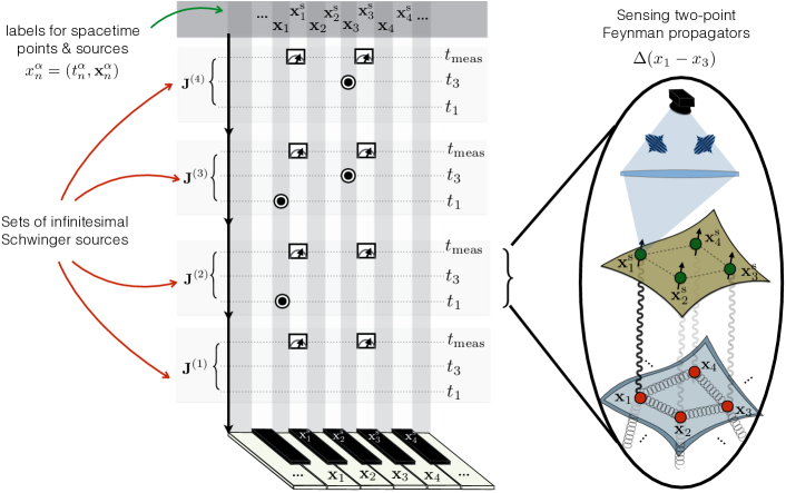
Figure 2: Schematic representation of the quantum sensing for Feynman propagators: The different indexes for the lattice sites ${\bf x}\in\Lambda_{\rm s}$, as well the corresponding $\mathbb{Z}_{2}$ sensors labelled by ${\bf x}^{\rm s}$, are mapped onto the keys of a piano. The set of pulse sequences $\mathbf{J}^{(m)}$ that couple the sensors to the field (14) corresponds to a piano score that indicates the sequence of keys (sensors) that must be pressed (coupled to the field) at different instants of time to produce a melody (spin-parity measurement) that encodes the relevant information about the Feynman propagators.

Let us now introduce the lattice $\mathbb{Z}_{2}$ Schwinger sources (6) by attaching a spin-1/2 quantum sensor $\sigma^{\alpha}_{{\bf x}}$ to each lattice point ${\bf x}\in\Lambda_{\ell}$, and defining a lattice Schwinger field $J^{\alpha}_{{\bf x}}(t)$. Accordingly, we have to supplement the above Hamiltonian of the lattice field theory with

$$H\to H_{J}=H+H_{\sigma}-\sum_{\alpha}\sum_{{\bf x}\in\Lambda_{\ell}}a^{d}J^{\alpha}_{{\bf x}}(t)\phi({\bf x})\sigma^{\alpha}_{{\bf x}},$$ (23)

where the dynamics of the sensors is governed by

$$H_{\sigma}=\sum_{{\bf x}\in\Lambda_{\ell}}a^{d}\delta\epsilon(\sigma^{0}_{{\bf x}}-P_{{\bf x}}),$$ (24)

and $P_{{\bf x}}$ projects onto the ground state of the sensor at lattice site ${\bf x}\in\Lambda_{\ell}$. Considering a Ramsey-type scheme $J^{\alpha}_{{\bf x}}=J_{{\bf x}}(t)(\delta_{\alpha,0}-\delta_{\alpha,3})/2$, the time-evolution operator (9) on the lattice can be expressed as

$$U_{J}(t,t_{0})=\mathsf{T}\left\{{\rm e}^{-{\rm i}(t-t_{0}){H}_{0}}\right\}\mathsf{T}\left\{{\rm e}^{+{\rm i}\int_{t_{0}}^{t}{\rm d}t^{\prime}\sum_{{\bf x}\in\Lambda_{\ell}}a^{d}J_{{\bf x}}(t)\phi_{\rm H}(t^{\prime},{\bf x})P_{{\bf x}}}\right\},$$ (25)

where $H_{0}=H+H_{\sigma}$ describes the uncoupled evolution of the self-interacting lattice field and the $\mathbb{Z}_{2}$ sensors. Considering an initial maximally-entangled state for the lattice sensors

$$\ket{\Psi(t_{0})}=\ket{\Omega}\otimes\frac{1}{\sqrt{2}}\left(\prod_{{\bf x}\in\Lambda_{\ell}}\sigma^{0}_{{\bf x}}+\prod_{{\bf x}\in\Lambda_{\ell}}\sigma^{1}_{{\bf x}}\right)\ket{0_{\sigma}},$$ (26)

we find that the corresponding spin-parity observable $\mathsf{P}[J,a]=\bra{\Psi(t_{0})}U_{J}^{\dagger}\prod_{{\bf x}\in\Lambda_{\ell}}\sigma^{1}_{{\bf x}}U_{J}\ket{\Psi(t_{0})}$ can be expressed as

$$\mathsf{P}[J,a]=\textstyle\frac{1}{2}{\rm e}^{{\rm i}(t-t_{0})\sum_{\bm{x}\in\Lambda_{\ell}}a^{d}\delta\epsilon}\mathsf{Z}[J,a]+{\rm c.c.},$$ (27)

where we have introduced the lattice generating functional

$$\mathsf{Z}[J,a]=\bra{\Omega}\mathsf{T}\left\{{\rm e}^{{\rm i}\int_{t_{0}}^{t}{\rm d}t^{\prime}\sum_{{\bf x}\in\Lambda_{\ell}}a^{d}J_{{\bf x}}(t^{\prime})\phi_{\rm H}(t^{\prime},{\bf x})}\right\}\ket{\Omega}.$$ (28)

The corresponding Feynman propagators $G^{(n)}_{{\bf x}_{1},\cdots{\bf x}_{n}}(t_{1},\cdots,t_{n})$ can be obtained by functional differentiation, as described in the continuum version (13), where one must consider again $t-t_{0}>{\rm max}\{|t_{i}-t_{j}|,\hskip 4.30554pt\forall\hskip 2.15277pti,j=1,\cdots,n\}$ to approximate the remote-past to distant-future conditions. We recall that a set ${\mathbf{J}}^{(m)}$ of point-like sources (14) would be required, such that one can reconstruct the discretization of the functional derivatives by the set of measured parities.

This lattice version offers a very vivid image of our quantum sensing apparatus as a piano (see Fig. 2). Let us label the $|\Lambda_{\ell}|$ lattice sites with an integer that maps each site to a particular key of a piano. The list $\mathbf{J}^{(m)}$, which describes the sequence of pulses that couple the sensors to the field (14), can be interpreted as a piano score that indicates the sequence of keys (sensors) that must be pressed (coupled to the field) at different instants of time to produce a melody (spin parity) that encodes the relevant information about the Feynman propagators.

Following book_lattice , the lattice generating functional (28) in the non-interacting limit, $\mathcal{V}(\phi)=0$, becomes $\mathsf{Z}_{0}[J,a]={\rm exp}\{-\textstyle\frac{1}{2}\int{\rm d}x^{0}\int{\rm d}y^{0}\sum_{\bm{x},\bm{y}\in\Lambda_{\ell}}a^{2d}J(x)\Delta_{0}({x}-{y},a)J(y)\}$, where

$$\Delta_{0}({x}-{y},a)=\!\!\int\frac{{\rm d}p^{0}}{2\pi}\sum_{{\bf p}\in{\rm BZ}}\frac{{\rm i}{\rm e}^{{\rm i}{p(x-y)}}}{(p^{0})^{2}-m_{0}^{2}-\sum_{\alpha}\left(\frac{2}{a}\sin\left(\frac{a}{2}p_{\alpha}\right)\right)^{2}},$$ (29)

is the single-particle Feynman propagator, and we have introduced the Brillouin zone ${\rm BZ}=[-\frac{\pi}{a},\frac{\pi}{a})^{\times^{d}}$. From this expression, the corresponding propagator in momentum space

$$\Delta_{0}(p,a)=\frac{{\rm i}}{(p^{0})^{2}-m_{0}^{2}-\sum_{\alpha}\big{(}\frac{2}{a}\sin\left(\frac{a}{2}p_{\alpha}\right)\big{)}^{2}},$$ (30)

has a well-defined continuum limit. Removing the lattice cut-off, this propagator coincides with that of the free scalar Klein-Gordon QFT $\lim_{a\to 0}\Delta_{0}(p,a)={\rm i}/(p^{2}-m_{0}^{2})$ qft_book , where $p^{2}=(p^{0})^{2}-{\bf p}^{2}$. Note that the pole of the propagator at ${\bf p}^{2}=0$, which determines the physical mass $m$ of the scalar particle, coincides in this case with the bare mass $m_{0}$ of the original field theory (1).

As noted below Eq. (22), the situation is more involved when $\mathcal{V}(\phi)\neq 0$, since the bare parameters of the theory must depend on the cut-off to cure the UV divergences. The particular cut-off-dependence of the bare parameters is determined by requiring that the physical observables at the length scale of interest are not modified when the number of high-energy modes, describing fluctuations at much smaller length scales, is increased in the continuum limit $\Lambda_{\rm c}^{-1}\to 0$. Since $a$ (or $\Lambda_{c\rm}^{-1}$) is a length (or inverse energy) scale, and hence not dimensionless, taking the continuum limit should always be understood in the sense that $\xi/a\to\infty$. Here, $\xi$ sets the relevant length scale of interest in such a way that physical quantities become independent of the underlying lattice structure.

We will discuss this point in more detail below, but let us first introduce a particular AMO platform that can be used as an AQS of a self-interacting scalar QFT on the lattice. Regarding the lattice counterpart of the sensing protocols for other continuum QFTs discussed in Subsec. II.5, a similar approach to the one presented in this section would hold for N-component scalar fields and fermion fields with bilinear sources. On the other hand, extending our sensing protocol to lattice gauge fields is an open question that deserves further studies, especially in view of the recent progress towards the quantum simulation of lattice gauge theories dqs_lattice_gauge_theories ; dqs_qft_gauge_U(1)_qlinks ; dqs_lattice_gauge_theories ; dqs_qft_SU(2)_qlinks ; aqs_qft_gauge_U(1)_qlinks ; aqs_QED ; aqs_qft_gauge_U(1)_qlinks ; aqs_qft_fermions_U(1)_qlinks ; aqs_qft_fermions_SU(2)_qlinks ; aqs_qft_fermions_U(1)_qlinks ; aqs_qft_fermions_SU(2)_qlinks ; zohar_review .

III.2 Trapped-ion quantum simulators of the $\lambda\phi^{4}$ QFT

The possibility of trapping atomic ions by electromagnetic fields has allowed to test the predictions of quantum mechanics at the single-atom level ions_rmp ; wineland_nobel . After the seminal work by Cirac and Zoller cz_gates , it was understood that operating with several ions would allow for quantum information processing ions_qc_review , turning trapped ions into a very promising route towards quantum error correction color_code_ions . Prior to the development of a large-scale fault-tolerant quantum computer based on trapped ions, one may exploit the experimental setup for quantum simulations qs_ions . As argued in the introduction, with few notable exceptions of DQS lgt_ions , the experimental emphasis has been placed on the quantum simulation of condensed-matter problems QS_trapped_ions . However, as discussed in this section, trapped ions also have the potential of becoming useful AQS of relativistic QFTs in a high-energy physics context.

The motion of a system of $N$ trapped atomic ions of mass $m_{\rm a}$ and charge $e$ can be described by the Hamiltonian

$$H_{m}=\sum_{i=1}^{N}\sum_{\alpha=x,y,z}\left(\frac{1}{2m_{\rm a}}p_{i\alpha}^{2}+\frac{1}{2}m_{\rm a}\omega_{\alpha}^{2}r_{i\alpha}^{2}\right)+\frac{e_{0}^{2}}{2}\sum_{i}\sum_{j\neq i}\frac{1}{|{\bf r}_{i}-{\bf r}_{j}|},$$ (31)

where we have introduced the position $r_{i\alpha}$ and momentum $p_{i\alpha}$ operators fulfilling $[r_{i\alpha},p_{j\beta}]={\rm i}\delta_{i,j}\delta_{\alpha,\beta}$, and the effective trapping frequencies $\{\omega_{\alpha}\}_{\alpha=x,y,z}$ in the pseudo-potential approximation ions_rmp . Here, $e_{0}^{2}=e^{2}/4\pi\epsilon_{0}$ is expressed in terms of the vacuum permittivity $\epsilon_{0}$, and we have set $\hbar=1$, which is customary in AMO physics since energies are then given by the frequency of the electromagnetic radiation used to excite a particular transition observed in spectroscopic measurements.

As a result of the competition between the Coulomb repulsion and the trap confinement, the ions can self-assemble in Coulomb crystals of different geometries when the temperatures get sufficiently low zigzag_ions . In this article, we shall be interested in linear and zigzag crystal configurations, which are routinely obtained in linear Paul traps zigzag_spectroscopy and, more recently, also in a combination of a Paul trap and an optical lattice ion_crystal_optical_lattices , which shall be referred to as a sub-wavelength Paul trap. In addition, the recent experiments showing the crystallization of ion rings in segmented ring traps ion_ring could also explore different crystal configurations.

In the harmonic-crystal approximation, one considers small vibrations around the equilibrium positions ${\bf r}_{i}={\bf r}_{i}^{0}+\sum_{\alpha}q_{i,\alpha}{\bf e}_{\alpha}$, and obtains a model of coupled harmonic oscillators that leads to the vibrational normal modes of the Coulomb crystal modes_ion_crystal . This approximation, however, cannot account for the motional dynamics of the ions close to a structural transition between different crystalline structures. In particular, when $\omega_{y}\gg\omega_{x},\omega_{z}$, a structural change between a linear ion chain and a zigzag ladder occurs as one lowers $\omega_{x}$ below a critical value $\omega_{\rm c}$ via a second-order phase transition spt_ions_molecular_dynamics . This phase transition can be understood by an effective Landau model landau_zigzag , which identifies the transverse zigzag distortion where neighbouring ions vibrate in anti-phase as a soft mode. For $\omega_{x}<\omega_{\rm c}$, the transverse phonons condense in a different ladder structure by spontaneously breaking a $\mathbb{Z}_{2}$ inversion symmetry. Not only is this theory in accordance with previous static predictions spt_ions_molecular_dynamics , but also serves as the starting point for studies of non-equilibrium dynamics of the crystal across the phase transition kibble_zurek_ions .

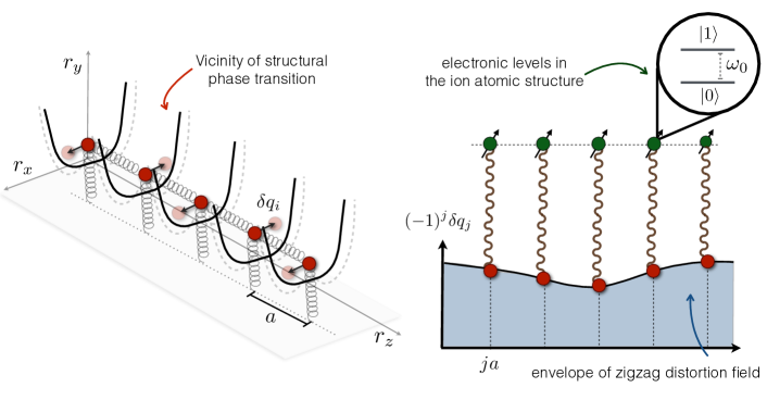
Figure 3: Effective $\lambda\phi^{4}$ QFT for ion crystals and quantum sensing scheme: (left) In the vicinity of the linear to zigzag structural phase transition of a trapped-ion crystal, the transverse zigzag vibrations yield the soft mode that contains the universal properties of the transition. (right) The slowly-varying envelop of the zigzag distortion (32) allows to develop a gradient expansion that leads to the effective $\lambda\phi^{4}$ QFT. By exploiting two electronic levels of the ions, and a state-dependent dipole force (49), one can infer the generating functional of the QFT.

An effective low-energy theory for the linear-to-zigzag transition can be derived as follows, both for ion rings effective_phi_4 and inhomogeneous linear crystals spin_peierls_ions . Let us rewrite the equilibrium positions as ${\bf r}_{i}^{0}=a\tilde{\bf r}_{i}^{0}$, where $a$ is a relevant length scale in the problem. For the sub-wavelength Paul traps or for ring traps, $a$ is the uniform lattice spacing, whereas for linear Paul traps where the crystals are inhomogeneous, $a=(e_{0}^{2}/m_{\rm a}\omega_{z}^{2})^{1/3}$ is simply a length scale with the order of magnitude of the average lattice spacing. We know from the previous discussion that the low-energy physics will be governed by excitations around the soft zigzag mode, which corresponds to momentum $k_{\rm s}=\pi/a$ in a ring trap (see Fig. 3). In analogy with other problems in condensed matter, see e.g. affleck_notes , one puts a cut-off around this momentum, considering only low-energy excitations that should capture the long-distance physics. This amounts to rewriting the zigzag distortion as $q_{j,x}={\rm e}^{{\rm i}k_{\rm s}ja}\delta q_{j}$, where $\delta q_{j}$ is a displacement that is slowly-varying on the scale of the lattice spacing which only contains the modes near $k_{\rm s}$. This can be generalized to situations without the periodicity of the ring by simply defining

$$q_{j,x}=(-1)^{j}\delta q_{j}.$$ (32)

A gradient expansion $\delta q_{j}\approx\delta q_{i}+(\tilde{\bf r}_{j}^{0}-\tilde{\bf r}_{i}^{0})\partial_{i+1}\delta q_{i}$, where $\partial_{j}\delta q_{i}=(\delta q_{i}-\delta q_{j})$ fulfils $|\partial_{j}\delta q_{i}|\ll\delta q_{i}$ due to its slowly-varying condition, yields the following Hamiltonian

$$H_{m}\approx\!\sum_{i}\!\left(\!\frac{m_{\rm a}}{2}\left(\partial_{t}\delta q_{i}\right)^{2}\!+\!\frac{\tilde{k}_{i}}{2}(\partial_{i+1}\delta q_{i})^{2}+\frac{k_{i}}{2}\delta q_{i}^{2}\!+\frac{u_{i}}{4}\delta q_{i}^{4}\!\right)\!.$$ (33)

Here, we have introduced a local spring constant and self-interaction coupling for each transverse displacement

$$k_{i}=m_{\rm a}\omega_{x}^{2}\left(1-\textstyle\frac{1}{2}\kappa\zeta_{i}(3)\right),\hskip 4.30554ptu_{i}=\frac{3}{4a^{2}}m_{\rm a}\omega_{x}^{2}\kappa\zeta_{i}(5),$$ (34)

where $\zeta_{i}(n)=\sum_{l\neq i}[(-1)^{i}-(-1)^{l}]^{n-1}|\tilde{{\bf r}}_{i}^{0}-\tilde{\bf r}_{l}^{0}|^{-n}$, and $\kappa=e_{0}^{2}/m_{\rm a}\omega_{x}^{2}a^{3}$ is a dimensionless constant. Additionally, the spring constants between neighbouring displacements are

$$\tilde{k}_{i}=m_{\rm a}\omega_{x}^{2}\sum_{l\neq i}\frac{(-1)^{l+i+1}\kappa}{2|\tilde{\bf r}_{i}^{0}-\tilde{\bf r}_{l}^{0}|}.$$ (35)

The Hamiltonian in Eq. (33) already resembles the lattice field theory of a $D=1+1$ Klein-Gordon QFT (22), where the underlying ion crystal plays the role of the $d=1$ lattice

$$\Lambda_{\ell}=\{{\rm x}:{\rm x}/a=\tilde{\bf r}_{i}^{0},\forall i=1,\cdots N\}.$$ (36)

We thus specialize to $D=1+1$ dimensions, in which, as noted below Eq. (1), the engineering dimension of the scalar field is $d_{\phi}=(D-2)/2=0$. In order to define the correct scalar field operators, one has to pay special attention to the different system of units in equations (22) and (33). Essentially, we need to identify the speed of sound that will play the role of the effective speed of light in the relativistic QFT. Since the scalar field must be dimensionless, we start by defining the following lattice operators

$$\tilde{\phi}({\rm x})=\frac{1}{a}\delta q_{i},\hskip 8.61108pt\tilde{\pi}({\rm x})=m_{\rm a}\partial_{t}\delta q_{i},$$ (37)

which show the desired commutation relations $[\tilde{\phi}({\rm x}),\tilde{\pi}({\rm y})]={\rm i}\delta_{\rm x,y}/a$. The lattice Hamiltonian (33) can then be expressed as $H_{m}=H_{0}+V$, where we have introduced

$$H_{0}=\sum_{{\rm x}\in\Lambda_{\ell}}\!\!a\hskip 0.86108pt\!\left(\frac{\tilde{\pi}({\rm x})^{2}}{2m_{\rm a}a}+\frac{\tilde{k}_{i}a^{3}}{2}(\nabla\tilde{\phi}({\rm x}))^{2}\right),$$ (38)

and used the operator $\nabla\tilde{\phi}({\rm x})=\left(\tilde{\phi}({\rm x}+a{{u}_{x}})-\tilde{\phi}({\rm x})\right)/a$. This part can be rewritten in terms of

$$H_{0}=\sum_{{\rm x}\in\Lambda_{\ell}}\!\!a\hskip 0.86108pt\frac{c_{\rm x}}{2}\!\left(\frac{\tilde{\pi}({\rm x})^{2}}{K_{\rm L,x}}+K_{\rm L,x}(\nabla\tilde{\phi}({\rm x}))^{2}\right),$$ (39)

where we have introduced an effective sound velocity

$$c_{\rm x}=a\sqrt{\frac{\tilde{k}_{i}}{m_{\rm a}}},\hskip 8.61108pt$$ (40)

which has the correct dimensions $[c_{\rm x}]=[\tilde{k}_{i}a^{2}]^{1/2}\cdot[m_{\rm a}]^{-1/2}=(\mathsf{ML^{2}T^{-2}}\cdot\mathsf{M^{-1}})^{1/2}={\mathsf{LT}}^{-1}$. Additionally, we have also introduced the so-called stiffness or Luttinger parameter

$${K}_{\rm L,x}=a^{2}\sqrt{\tilde{k}_{i}m_{\rm a}},$$ (41)

which appears in the theory of bosonization and controls the power-law decay of correlations in Luttinger liquids cm_book . Reintroducing Planck’s constant, ${K}_{\rm L,x}=\frac{a^{2}}{\hbar}\sqrt{\tilde{k}_{i}m_{\rm a}}$, this Luttinger parameter turns out to be dimensionless ${K}_{\rm L,x}=([\tilde{k}_{i}a^{2}]/[\hbar^{2}/m_{\rm a}a^{2}])^{1/2}=(\mathsf{ML^{2}T^{-2}}/\mathsf{ML^{2}T^{-2}})^{1/2}=1$. In order to arrive at the standard definition of a $\lambda\phi^{4}$ QFT on the lattice (22), we perform an additional rescaling of the lattice field operators that preserves the commutation relations

$${\phi}({\rm x})=\sqrt{{K}_{\rm L,x}}\tilde{\phi}({\rm x}),\hskip 8.61108pt{\pi}({\rm x})=\frac{1}{\sqrt{{K}_{\rm L,x}}}\tilde{\pi}({\rm x}).$$ (42)

This leads to the desired lattice field theory

$$H_{0}=\sum_{{\rm x}\in\Lambda_{\ell}}\!\!a\hskip 0.86108pt\frac{c_{\rm x}}{2}\!\left({\pi}({\rm x})^{2}+(\nabla{\phi}({\rm x}))^{2}\right),$$ (43)

which yields the desired QFT of a 1+1 free massless scalar boson $H_{0}=\int{\rm dx}\frac{c_{\rm x}}{2}\!\left({\pi}({\rm x})^{2}+(\partial_{\rm x}{\phi}({\rm x}))^{2}\right)$ in the continuum limit $a\to 0$. Note that, as a consequence of the inhomogeneous lattice spacing in a linear Paul trap, all these parameters have inhomogeneities around the edges of the ion chain, while they become constants for ring traps and sub-wavelength Paul traps, where the lattice spacing is homogeneous.

In addition to these terms, the remaining part of the lattice Hamiltonian (33) yields a mass term and a self-interaction of the scalar field

$$V=\sum_{{\rm x}\in\Lambda_{\ell}}\!\!a\left(\frac{m_{0,\rm x}^{2}}{2}\phi({\rm x})^{2}+\frac{{\lambda}_{\rm x}}{4!}{{\phi}}({\rm x})^{4}\right).$$ (44)

Here, we have introduced the bare mass and coupling strength

$${m}^{2}_{0,\rm x}=\frac{k_{i}a}{K_{\rm L,x}},\hskip 8.61108pt{\lambda}_{\rm x}=\frac{6u_{i}a^{3}}{K_{\rm L,x}^{2}},$$ (45)

which fulfil $[a{m}^{2}_{0,\rm x}]=[a\lambda_{\rm x}]=\mathsf{ML^{2}T}^{-2}$ after taking into account the lattice spacing $a$ from the lattice sum in Eq. (44), and thus display the expected units of energy. In Landau’s mean-field theory, ${m}_{0,\rm x}^{2}<0$, ${\lambda}_{\rm x}>0$ signals a phase transition where $\langle{\phi}({\rm x})\rangle\neq 0$ is achieved by spontaneously breaking the $\mathbb{Z}_{2}$ symmetry ${\phi}({\rm x})\to-{\phi}({\rm x})$ in the effective lattice field theory (46). This is exactly in agreement with previous estimates of the linear-to-zigzag phase transition in ion crystals, both in homogeneous and inhomogeneous cases. However, the mean-field approach predicts a wrong scaling behavior in the vicinity of the critical point, which could be tested experimentally with the protocol presented in this work.

In the context of relativistic QFTs (1), we should recover Lorentz invariance in the continuum limit. This can be achieved for the whole ion crystal in ring traps or sub-wavelength Paul traps, or by restricting to the homogeneous bulk of the crystal in a linear Paul trap. In these cases, we can set the corresponding natural units $c=1$, such that the low-energy Hamiltonian governing the linear-to-zigzag instability in ion crystals becomes equivalent to the $D=1+1$ lattice Klein-Gordon field (22) with quartic interactions

$$H_{m}=\!\sum_{{\rm x}\in\Lambda_{\ell}}\!a\left(\textstyle\frac{1}{2}\pi({\rm x})^{2}+\textstyle\frac{1}{2}(\nabla\phi({\rm x}))^{2}+\frac{m_{0}^{2}}{2}\phi({\rm x})^{2}+\frac{\lambda}{4!}\phi({\rm x})^{4}\right).$$ (46)

Note that with all these definitions, we have made sure that the classical mass dimensions $d_{\phi}=0$, while the couplings have $d_{m_{0}^{2}}=2=d_{\lambda}$. Finally, we also note that in numerical lattice simulations and formal renormalization group (RG) calculations, one typically defines dimensionless couplings $\tilde{m}_{0}^{2}=m_{0}^{2}a^{2}$ and $\tilde{\lambda}=\lambda a^{2}$. In the so-called lattice units, the lattice constant disappears from the above Hamiltonian, such that taking the continuum limit corresponds to modifying the dimensionless couplings. As remarked at the end of the previous subsection, taking the continuum limit does not require changing the actual inter-ion distance, but is instead achieved by setting these dimensionless couplings close to a critical point where $\xi/a\to\infty$, and physical quantities become independent of the underlying lattice structure.

According to this discussion, trapped-ion crystals can be used as AQSs of the lattice $\lambda\phi^{4}$ QFT (46), where the fields (42) are proportional to the zigzag displacement (32) via Eq. (37). The proportionality parameter, as well as the bare mass and self-interaction strength of the QFT are expressed in terms of microscopic parameters (34)-(35) via Eqs. (40)-(41) and (45). We note that this approach differs from a non-canonical transformation introduced in hbar_zigzag , which yields a similar Hamiltonian (46) after a particular rescaling of Eq. (33). However, an effective Planck constant $\hbar$ depending on the model parameters must be introduced to maintain the required commutation relations. This leads to important differences in the renormalization with respect to the standard approach for the $\lambda\phi^{4}$ theory, which shall be discussed below.

As advanced in the introduction, the usefulness of an AQS does not only depend on the accuracy with which it behaves according to the model of interest, e.g. a self-interacting scalar QFT, but also on the measurement strategies to extract the relevant properties of this simulated model. In our trapped-ion scenario, the position of the ions $\langle{\bf r}_{i}\rangle$ is routinely measured by driving a transition between two electronic levels and collecting the spontaneously-emitted photons in a camera ions_rmp , such that the expectation value $\langle\phi({\rm x})\rangle$ could be inferred from the above relations. This can be used to locate the critical point of the $\mathbb{Z}_{2}$ phase transition when a vacuum expectation value $\langle\phi({\rm x})\rangle\neq 0$ is developed, which would require and accurate measurement of the zigzag ion positions zigzag_spectroscopy . However, in the symmetry-broken phase, the zigzag crystal will also experience micromotion (i.e. additional fast oscillations synchronous with the driving fields of the Paul trap) that go beyond the pseudo-potential approximation, such that other spectroscopic observables can be modified with respect to the static situation zigzag_spectroscopy . In the present context, the pseudo-potential approximation is used to derive Eq. (46), and it would thus be safer for the accuracy of the AQS to perform experiments in the symmetry unbroken phase, where these standard fluorescence measurements cannot be used to determine the properties of the QFT. For instance, if one is interested in simulating a massive scalar particle with the AQS, one would like to know how the bare mass gets renormalized as a consequence of the self-interactions, or how a collection of massive scalar particles would scatter off each other due to these interactions. In the following section, we show that the protocol to measure the generating functional $\mathsf{Z}[J,a]$ (28), which contains the information about all of these properties, and has an experimental realization that is feasible with state-of-the art control over trapped-ion crystals.

III.3 Trapped-ion sensors for the generating functional

The Hamiltonian (31) describes the motional degrees of freedom of a collection of trapped ions. Additionally, the ions have an internal atomic structure with its own independent dynamics. We can exploit such internal degrees of freedom as the quantum sensors introduced in Sec. II (see Fig. 3).

We will consider external laser beams that only couple to a pair of such internal states $\{\ket{0_{i}},\ket{1_{i}}\}$, which have a transition of frequency $\omega_{0}$. The Hamiltonian governing this internal dynamics is simply $H_{in}=\sum_{i=1}^{N}\omega_{0}(\sigma^{0}_{i}-P_{i})$, where $\sigma^{0}_{i}=\mathbb{I}=\ket{0_{i}}\bra{0_{i}}+\ket{1_{i}}\bra{1_{i}}$, and $P_{i}=\ket{0_{i}}\bra{0_{i}}$ is the projector onto the lowest-energy internal state. This Hamiltonian is directly equivalent to the quantum-sensor Hamiltonian (24) using the crystal as the underlying lattice (36), such that

$$H_{in}=\sum_{{\rm x}\in\Lambda_{\ell}}\!a\hskip 0.43057pt\delta\epsilon(\sigma^{0}_{{\rm x}}-P_{{\rm x}}),\hskip 8.61108pt\delta\epsilon=\frac{\omega_{0}}{a}.$$ (47)

In order for these electronic levels to act as quantum sensors of the QFT generating functional, we need to induce a coupling of the form (23), such that these probes act as the $\mathbb{Z}_{2}$ Schwinger sources introduced in Sec. II. We consider the so-called state-dependent dipole forces sd_force , which can be obtained from a pair of laser beams of frequency $\omega_{\rm L,1},\omega_{\rm L,2}$ that couple the internal state $\ket{0}_{i}$ off-resonantly to an auxiliary excited state from the atomic level structure. Using selection rules cats_ions , and working in the far off-resonant regime, the laser-ion coupling can be expressed as a crossed-beam ac-Stark shift

$$H_{l-i}=\sum_{i}\frac{\Omega_{\rm L}}{2}P_{i}{\rm e}^{{\rm i}(\Delta{\bf k}_{\rm L}\cdot{\bf r}_{i}-\Delta\omega_{\rm L}t)}+{\rm H.c.},$$ (48)

where we have introduced a two-photon Rabi frequency $\Omega_{\rm L}$, and the wave-vector (frequency) difference of the laser beams $\Delta{\bf k}_{\rm L}=\Delta{\bf k}_{\rm L,1}-\Delta{\bf k}_{\rm L,2}$ ($\Delta{\omega}_{\rm L}=\Delta{\omega}_{\rm L,1}-\Delta{\omega}_{\rm L,2}$). After expressing the ion position operator in terms of the vibrations ${\bf r}_{i}={\bf r}_{i}^{0}+\sum_{\alpha}q_{i,\alpha}{\bf e}_{\alpha}$, one sees directly that if the overlapping beams propagate along $\Delta{\bf k}_{\rm L}||{\bf e}_{x}$, the radiation will couple to the desired zigzag distortion (32). Moreover, a Taylor expansion in the Lamb-Dicke regime, $|\langle\Delta{\bf k}_{\rm L}\cdot{\bf e}_{x}q_{i,x}\rangle|\ll 1$, shows that the leading-order contribution from the laser-ion interaction (48), for $|\Omega_{\rm L}|\ll\Delta\omega_{\rm L}\sim\omega_{x}$, will be a state-dependent dipole force that excites the zigzag distortion when the internal state of the ions is in $\ket{0_{i}}$, namely

$$H_{l-i}=\sum_{i}g_{i}(t)P_{i}\delta q_{i},\hskip 4.30554ptg_{i}(t)=\Omega_{\rm L}(\Delta{\bf k}_{\rm L}\cdot{\bf e}_{x}a)(-1)^{i}\sin{\Delta\omega_{\rm L}t}.$$ (49)

We will also assume that the laser beams can be split into individual addressing beams that couple to any ion in the crystal, such that $\Omega_{\rm L}\to\Omega_{{\rm L},i}(t)$ can be controlled individually, e.g. switched on/off, by controlling the intensity of each of the addressing beams as achieved experimentally in ind_addressing_raman . Using this expression in combination with Eqs. (46) and (47), we arrive at the desired lattice field theory with $\mathbb{Z}_{2}$ Schwinger sources (23), namely

$$H_{J}=H_{m}+H_{\rm in}-\sum_{\alpha}\sum_{{\bf x}\in\Lambda_{\ell}}aJ^{\alpha}_{{\rm x}}(t)\phi({\rm x})\sigma^{\alpha}_{{\rm x}},$$ (50)

where we have introduced the source fields

$$J^{\alpha}_{{\rm x}}(t)=\frac{J_{{\rm x}}(t)}{2}(\delta_{\alpha,0}-\delta_{\alpha,3}),\hskip 8.61108ptJ_{{\rm x}}(t)=\frac{g_{i}(t)}{\sqrt{K_{\rm L,x}}}.$$ (51)

Note that, by using the dimensional analysis of the previous section, the source fields also have the desired mass dimensions $d_{J}=2$.

Provided that one can prepare the initial state of the ions according to Eq. (8), and measure the parity observable in Eq. (10), it becomes possible to implement the protocol presented in Sec. II, inferring the generating functional $\mathsf{Z}[J,a]$ of the particular trapped-ion $\lambda\phi^{4}$ QFT. For the $T=0$ case, the state preparation would rely on an adiabatic evolution that starts far away from the structural phase transition, and utilizes laser cooling to prepare a state very close to the vacuum of the transverse vibrations. Then, the trap parameters would be adiabatically modified by approaching the critical point of the linear-to-zigzag transition, but remaining in the symmetry-preserved phase. For the $T\neq 0$ case, one would perform laser cooling directly in the interacting regime, during a time that is large enough so that the motional degrees of freedom thermalize. Then, the internal state has to be prepared in a GHZ state, which can be accomplished using gates mediated by the phonons that are not involved in the structural phase transition entangled_ions . We remark that the high fidelities already achieved in the experimental preparation of large GHZ states monz_14_qubit_entanglement make trapped ions a very promising AMO setup for the implementation of this proposed protocol.

Before closing this subsection, let us note that the simplified protocols of Sec. II to measure any Feynman propagator could also be implemented in this trapped-ion scenario, provided that one has the aforementioned addressability in the laser-ion couplings ind_addressing_raman . In such case, the state in Eq. (15) or (18) could be prepared along similar lines, and the required switching of instantaneous sources to estimate the functional derivatives (13) would also be available. The measurement corresponds to a multi-spin correlation function of the type that is routinely measured through the state-dependent fluorescence of the ions ions_rmp . Prior to driving the cycling transition and collecting the emitted photons, one should apply a global single-qubit rotation by driving the so-called carrier transition ions_rmp . We note that the measurements have to be repeated for different values of the field-sensor couplings to infer the propagators via the discretized derivatives (17). During these additional repetitions, one must avoid slow drifts in the microscopic trapped-ion parameters. An advantage in this regard is that our proposal focuses on the propagator of the vibrations, which will be 1-2 orders of magnitude faster than experiments on the propagation of spin excitations in effective spin-spin models with trapped ions propagation_spin_excitations_ions , where analogous measurements are typically done.

III.4 Renormalization and the continuum limit

As advanced in the sections above, using the lattice generating functional $\mathsf{Z}[J,a]$ (28) to learn about the continuum QFT (1) requires letting $a\to 0$, and removing the lattice cut-off $\Lambda_{\rm c}\propto a^{-1}\to\infty$. This continuum limit must be performed without affecting the physical observables at the length scale of interest. Note also that the Schwinger sources should be spaced at the same physical distance as the ’continuum limit’ is taken. For instance, in the context of the trapped-ion quantum simulator (46), such an observable will be the parity operator (12), which encodes the information about the Feynman propagators (5) and thus the physical mass $m$ of the scalar particles. In this case, the relevant length scale for the scalar fields (42) is set by the envelope of the zigzag distortion (32), which varies on a much larger scale than the lattice spacing. In the generic situation, we can safely send $a\to 0$ without altering the long-wavelength phenomena, but we must ensure that our calculations will not suffer from possible UV divergences as further high-energy modes are included by this process. In practice, this requires allowing the bare couplings of the theory $\{g_{i}\}$, e.g. $\{m_{0}^{2},\lambda\}$ in Eq. (46), to flow with the lattice cut-off $\{g_{i}(\Lambda_{\rm c})\}$ in such a way that one stays on the ’line of constant physics’. In the AQS, this would mean that the value of the microscopic parameters, which control the effective lattice parameters such as the bare mass, have to be tuned to particular values in order to obtain the renormalized physical mass of the particles at the scale of interest, which will be independent of the cut-off and different from the bare mass. The renormalization group is essential to understand this flow and, with it, the nature of such a continuum limit rg_hollowod .

At the UV limit $\{g_{i}(\infty)\}$, the resulting QFT must belong to the so-called critical surface, i.e. the couplings must lie at the domain of attraction of a fixed point of a transformation that changes the cut-off scale. To preserve the physics at the length-scale of interest, one has to fix a one-parameter set of field theories with different cut-offs $\{g_{i}(\Lambda_{\rm c})\}$ that connects to such a well-defined UV limit. This is achieved by specifying the relevant couplings $\{g_{i}^{\rm r}(\Lambda_{\rm c})\}\in\{g_{i}(\Lambda_{\rm c})\}$ that take us away from the critical surface as one moves from the UV towards the infra-red (IR) $\Lambda_{\rm c}\to 0$, approaching thus the length-scale of interest. The difficulty lies in identifying the possible RG fixed points and relevant couplings of a particular field theory. In this regard, the scalar QFT (1) with self-interactions $\mathcal{V}(\phi)=\sum_{n}g_{2n}\phi^{2n}/(2n)!$ and $D=4$ yields a very instructive scenario where the RG machinery can be developed in perturbation theory rg_hollowod ; wilson_rg . Typically, one starts from the so-called Gaussian fixed point, where $g_{2n}(\infty)=0$, and shows that it suffices to consider the flow of $g_{2}(\Lambda_{\rm c})$ and $g_{4}(\Lambda_{\rm c})$ to understand the continuum limit. This follows from simple dimensional analysis, since the so-called anomalous dimensions of the fields vanish at this fixed point, allowing one to realize that the higher-order couplings $\{g_{2n}(\Lambda_{\rm c})\}_{n>2}$ are all irrelevant, i.e. decrease as one moves towards the IR. At one loop in perturbation theory, $g_{2}(\Lambda_{\rm c})$ remains a relevant coupling, while $g_{4}(\Lambda_{\rm c})$ becomes irrelevant. Therefore, unless a different RG fixed point exists, the lattice regularization of the scalar QFT in $D=4$ only has a trivial non-interacting continuum limit. Using the so-called $\epsilon$ expansion, which allows for non-integer dimensions $D=4-\epsilon$, it is possible to find a non-trivial fixed point that would allow for an interacting and massive QFT in the continuum, the so-called Wilson-Fisher fixed point at finite $g_{2}(\infty)\neq 0,g_{4}(\infty)\neq 0$. However, this fixed point exists only for $\epsilon>0$ and thus $D<4$, suggesting the triviality of the lattice scalar QFT in $D=4$ wilson_rg ; triviality_lattice .

To go beyond the perturbative RG, numerical lattice simulations based on Monte Carlo methods become very useful book_lattice . The general strategy of lattice field theory simulations is to set the bare lattice couplings in the vicinity of a quantum critical point, where the correlation length $\xi\to\infty$ diverges, and one expects to recover the universal features of the QFT in the continuum limit $a\to 0$. In our context, $g_{2}(\Lambda_{\rm c})$ and $g_{4}(\Lambda_{\rm c})$ must be set in the vicinity of the $\mathbb{Z}_{2}$ quantum phase transition, which should be controlled by the scale-invariant fixed point of the RG transformation. The renormalized mass can be extracted from the numerical computation of propagators, whereas the renormalized interactions can be obtained from susceptibilities. This approach corroborates the triviality of the lattice scalar QFT in $D=4$ in non-perturbative regimes triviality_monte_carlo .

In the $D=2$ limit, which is the case of interest for the trapped-ion quantum simulator (46), the need of non-perturbative schemes is even more compelling. In this case, applying the above perturbative RG calculation around the Gaussian fixed point would show that all of the couplings $\{g_{2n}(\Lambda_{\rm c})\}_{n\geq 1}$ are relevant rg_hollowod , thus questioning the validity of the truncation implicit in Eq. (33) that is used to derive the effective QFT (46) from the microscopic Hamiltonian (31). In fact, in 1+1 dimensions, the field operators for a free scalar QFT have non-vanishing anomalous dimensions even in the absence of interactions, such that the simple dimensional analysis around the Gaussian fixed point is no longer valid. In this case, the tools of conformal field theory would be required to understand the RG flow of perturbations around the scale-invariant fixed point of a free scalar boson, as occurs for the sine-Gordon model cm_book . However, the particular perturbations of our self-interacting scalar QFT do not have simple conformal/scaling dimensions, and thus do not allow for a simple analytical approach. Accordingly, the existence of non-perturbative numerical methods becomes even more relevant in this situation. Recent results for this 1+1 scalar $\lambda\phi^{4}$ QFT, either based on Monte Carlo phi_4_1d_montecarlo and real-space renormalization group phi_4_1d_dmrg_mps methods on the lattice, or Hamiltonian truncation methods in a finite volume phi_4_1d_ham_truncation , have shown that the continuum limit of this QFT is controlled by a non-trivial fixed point corresponding to the Ising conformal field theory. These works show the power of the lattice approach to solve non-perturbative questions of the continuum QFT, such as the precise location of the $\mathbb{Z}_{2}$ quantum phase transition, i.e. the critical value of $\lambda/m^{2}$ where the scalar field acquires a vacuum expectation value. At a fundamental level, they also imply that perturbations $\{g_{2n}(\Lambda_{\rm c})\}_{n>2}$ around this fixed point, which are generated in the implicit RG process of looking into long-wavelength phenomena, are irrelevant. This justifies thus the validity of our truncation leading to Eq. (46). The hope of this manuscript is to show that, exploiting the proposed protocol to infer the full generating functional $\mathsf{Z}[J,a]$ of a QFT, trapped-ion AQS working in the vicinity of the linear-to-zigzag structural transition will serve as an alternative non-perturbative tool to explore such QFT questions.

IV Conclusions and outlook

In this work, we have presented a protocol to infer the normalized generating functional of a QFT by measuring a particular interferometric observable through a collection two-level quantum sensors. Generalizing the notion of Schwinger fields to serve simultaneously as sources and probes of the excitations of a quantum field, we have exploited the entanglement of the quantum sensors to show that a collective Ramsey-type response of the sensors contains all the information about the QFT generating functional. This, in turn, encodes in a compressed manner the relevant information of the interacting QFT (i.e. approximating functional derivatives by combining several measured responses can be used to decompress any $n$-point Feynman propagator, and thus any possible scattering or non-equilibrium real-time process). We have argued that this protocol finds a very natural realization in AQS on the lattice, and we have considered a trapped-ion realization of the $\lambda\phi^{4}$ QFT as a realistic example where experimental techniques can be applied to implement the generalized Schwinger sources, and infer the generating functional from resonance-fluorescence images. In this case, by performing experiments in the vicinity of the linear-to-zigzag structural phase transition, the trapped-ion AQS can in principle address non-perturbative questions regarding the nature of the fixed point that controls the QFT obtained in the continuum limit. During the completion of our work, S. P. Jordan et al. dqs_gen_func have shown that the algorithm for DQS of scattering in scalar QFTs dqs_qft_phi4 can be modified to obtain also the generating functional. Moreover, they argue that a particular instance of the generating functional, for a certain functional dependence of the source fields, cannot be efficiently estimated with any classical algorithm. It would be very interesting to study if similar complexity arguments can be carried over onto our AQS, which we believe presents an opportunity to measure the generating functional using current trapped-ion technology.

In general, understanding real-time dynamics of quantum fields, either in or out of equilibrium, is required in a wide range of physical applications. One important question in relativistic theories is far-from equilibrium dynamics and thermalization NONEQ . This is relevant e.g. for the end of inflation and preheating in the early universe PRE , or for the evolution during the early stages of heavy-ion collisions, resulting in the quark-gluon plasma (QGP) created at the Large Hadron Collider at CERN, or the Relativistic Heavy Ion Collider at BNL QGP-rev . In the former, the efficiency of particle production and transport of energy across different length scales determines the reheating temperature, whereas in the latter case the very creation of a thermal QGP depends on the ability of the highly non-equilibrium initial gluon fields to thermalize THERM . Since this dynamics takes place manifestly in real-time, it is often treated within classical approximations that are only valid for highly occupied modes HIC . It would hence be of the utmost interest to study similar, yet simplified, dynamical questions relevant for these situations using the protocol outlined in our work, and analyze e.g. the role of non-thermal fixed points FP using quantum dynamics in real time.

In thermal equilibrium, the information about spectral functions and other real-time correlators is also of interest. Even though they are related LeBellac to standard Euclidean correlation functions computable in lattice field theory, the analytical continuation from Euclidean to real time (or from Matsubara to real frequency) is a non-trivial process. The interest here lies e.g. in quasi-particle properties and other spectral features, such as thermal masses and widths, or in more ambitious questions related to hydrodynamic structure and transport at long wavelengths TRANS . It would be interesting to explore if similar questions can be addressed extending the present protocol for measurements of thermal current-current correlators in real time.

Acknowledgements.– We thank S. P. Kumar for useful discussions. This work has been supported by STFC grant ST/L000369/1. A.B. acknowledges support from Spanish MINECO Projects FIS2015-70856-P, and CAM regional research consortium QUITEMAD+. G. A. is supported by the Royal Society and the Wolfson Foundation. This work has been supported by STFC Grant No. ST/L000369/1.

References

- (1) E. Fradkin, Field Theories of Condensed Matter Physics (Cambridge University Press, Cambridge, 2013).
- (2) M. E. Peskin, and D. V. Schröder, An Introduction to Quantum Field Theory (Addison-Wesley, Reading, 1995).
- (3) See I. Bloch, J. Dalibard, and S. Nascimbene, Quantum simulations with ultracold quantum gases, Nat. Phys. 8, 267 (2012), and references therein.
- (4) See R. Blatt and C. F. Roos, Quantum simulations with trapped ions, Nat. Phys. 8, 277 (2012), and references therein.
- (5) R. P. Feynman, Simulating physics with computers, Int. J. Theor. Phys. 21, 467 (1982).
- (6) J. I. Cirac and P. Zoller, Goals and opportunities in quantum simulation, Nat. Phys. 8, 264 (2012).
- (7) M. Lewenstein, A. Sanpera, and V. Ahufinger, Ultracold Atoms in Optical Lattices: Simulating quantum many-body systems (Oxford University Press, Oxford, 2012).
- (8) S. Lloyd, Universal Quantum Simulators, Science 23, 1073 (1996).
- (9) D. Jaksch, C. Bruder, J. I. Cirac, C. W. Gardiner, and P. Zoller, Cold Bosonic Atoms in Optical Lattices, Phys. Rev. Lett. 81, 3108 (1998).
- (10) L. J. Garay, J. R. Anglin, J. I. Cirac, and P. Zoller, Sonic Analog of Gravitational Black Holes in Bose-Einstein Condensates, Phys. Rev. Lett. 85, 4643 (2000).
- (11) P. O. Fedichev and U. R. Fischer, Gibbons-Hawking Effect in the Sonic de Sitter Space-Time of an Expanding Bose-Einstein-Condensed Gas, Phys. Rev. Lett. 91, 240407 (2003); A. Retzker, J. I. Cirac, M. B. Plenio, and B. Reznik, Methods for Detecting Acceleration Radiation in a Bose-Einstein Condensate , Phys. Rev. Lett. 101, 110402 (2008).
- (12) Provided that one takes care of the so-called fermion doublers nielsen_nonomiya that appear in the naive discretization of a fermionic Dirac field.
- (13) H. B. Nielsen and M. Ninomiya, A no-go theorem for regularizing chiral fermions, Nuc. Phys. B 185, 20 (1990).
- (14) A. Bermudez, L. Mazza, M. Rizzi, N. Goldman, M. Lewenstein, and M. A. Martin-Delgado, Wilson Fermions and Axion Electrodynamics in Optical Lattices, Phys. Rev. Lett. 105, 190404 (2010); L. Mazza, A. Bermudez, N. Goldman, M. Rizzi, M. A. Martin-Delgado, and M. Lewenstein, An optical-lattice-based quantum simulator for relativistic field theories and topological insulators, New J. Phys. 14, 015007(2012).
- (15) S. P. Jordan, K. S. Lee, and J. Preskill, Quantum Algorithms for Quantum Field Theories, Science 336, 1130 (2012); ibid., Quantum computation of scattering in scalar quantum field theories, Quant. Inf. and Comp. 14, 1014 (2014).
- (16) J. Casanova, L. Lamata, I. L. Egusquiza, R. Gerritsma, C. F. Roos, J. J. García-Ripoll, and E. Solano, Quantum Simulation of Quantum Field Theories in Trapped Ions, Phys. Rev. Lett. 107, 260501 (2011).
- (17) L. García-Álvarez, J. Casanova, A. Mezzacapo, I. L. Egusquiza, L. Lamata, G. Romero, and E. Solano, Fermion-Fermion Scattering in Quantum Field Theory with Superconducting Circuits, Phys. Rev. Lett. 114, 070502 (2015).
- (18) J. I. Cirac, P. Maraner, and J. K. Pachos, Cold Atom Simulation of Interacting Relativistic Quantum Field Theories, Phys. Rev. Lett. 105, 190403 (2010).
- (19) J. Smit, Introduction to Quantum Fields on a Lattice (Cambridge Lecture Notes in Physics, Cambridge, 2003).
- (20) M. Stephanov, QCD phase diagram: an overview, PoS(LAT2006)024.
- (21) T. Byrnes and Y. Yamamoto, Simulating lattice gauge theories on a quantum computer, Phys. Rev. A 73, 022328 (2006).
- (22) H. P. Büchler, M. Hermele, S. D. Huber, M. P. A. Fisher, and P. Zoller, Atomic Quantum Simulator for Lattice Gauge Theories and Ring Exchange Models, Phys. Rev. Lett. 95, 040402 (2005); D. Marcos, P. Rabl, E. Rico, and P. Zoller, Superconducting Circuits for Quantum Simulation of Dynamical Gauge Fields, Phys. Rev. Lett. 111, 110504 (2013).
- (23) H. Weimer, M. Müller, I. Lesanovsky, P. Zoller, and H. P. Büchler, A Rydberg quantum simulator, Nat. Phys. 6, 382 (2010); L. Tagliacozzo, A. Celi, A. Zamora, and M. Lewenstein, Optical Abelian lattice gauge theories, Ann. Phys. 330, 160 (2013).
- (24) L.Tagliacozzo, A. Celi, P. Orland, M. W. Mitchell, and M. Lewenstein, Simulation of non-Abelian gauge theories with optical lattices, Nat. Comm. 4, 2615 (2013).
- (25) E. Kapit, and E. Mueller, Optical-lattice Hamiltonians for relativistic quantum electrodynamics, Phys. Rev. A 83, 033625 (2011); E. Zohar, and B. Reznik, Confinement and Lattice Quantum-Electrodynamic Electric Flux Tubes Simulated with Ultracold Atoms, Phys. Rev. Lett. 107, 275301 (2011); E. Zohar, J. Cirac, and B. Reznik, Simulating Compact Quantum Electrodynamics with Ultracold Atoms: Probing Confinement and Nonperturbative Effects, Phys. Rev. Lett. 109, 125302 (2012).
- (26) D. Banerjee, M. Dalmonte, M. Müller, E. Rico, P. Stebler, U.-J. Wiese, and P. Zoller, Atomic Quantum Simulation of Dynamical Gauge Fields Coupled to Fermionic Matter: From String Breaking to Evolution after a Quench, Phys. Rev. Lett. 109,175302 (2012); E. Zohar, J. Cirac, and B. Reznik, Simulating ( 2 + 1 )-Dimensional Lattice QED with Dynamical Matter Using Ultracold Atoms, Phys. Rev. Lett. 110, 055302 (2013).
- (27) D. Banerjee, M. Bögli, M. Dalmonte, E. Rico, P. Stebler, U.-J. Wiese, and P. Zoller, Atomic Quantum Simulation of U(N) and SU(N) Non-Abelian Lattice Gauge Theories, Phys. Rev. Lett. 110, 125303 (2013); E. Zohar, J. Cirac, and B. Reznik, Cold-Atom Quantum Simulator for SU(2) Yang-Mills Lattice Gauge Theory, Phys. Rev. Lett. 110, 125304 (2013).
- (28) See E. Zohar, J. I. Cirac, and B. Reznik, Quantum simulations of lattice gauge theories using ultracold atoms in optical lattices, Rep. Prog. Phys. 79, 014401 (2016), for additional references.
- (29) J. Schwinger, On the Green’s functions of quantized fields. I, Proc. Nat. Acad. Sci. 37, 452 (1951).
- (30) M. Gell-Mann and F. Low, Bound States in Quantum Field Theory, Phys. Rev. 84, 350 (1951).
- (31) See C. L. Degen, F. Reinhard, P. Cappellaro, Quantum sensing, arXiv:1611.02427 (2016), and references therein.
- (32) W. G. Unruh, Notes on black-hole evaporation, Phys. Rev. D 14, 870 (1976).
- (33) N. D. Birrel and P. C. Davies, Quantum Fields in Curved Space (Cambridge University Press, Cambridge, 1994).
- (34) A. Retzker, J. I. Cirac, and B. Reznik, Detecting Vacuum Entanglement in a Linear Ion Trap,Phys. Rev. Lett. 94, 050504 (2005); P. M. Alsing, J. P. Dowling, and G. J. Milburn, Ion Trap Simulations of Quantum Fields in an Expanding Universe, Phys. Rev. Lett. 94, 220401 (2005).
- (35) A. Recati, P.O. Fedichev, W. Zwerger, J. von Delft, P. Zoller, Atomic Quantum Dots Coupled to a Reservoir of a Superfluid Bose-Einstein Condensate, Phys. Rev. Lett. 94, 040404 (2005); M. Bruderer and D. Jaksch, Probing BEC phase fluctuations with atomic quantum dots, New J. Phys. 8, 87 (2006); C. Sabín, A. White, L. Hackermuller, and I. Fuentes, Impurities as a quantum thermometer for a Bose-Einstein condensate, Sci. Rep. 4, 6436 (2014); F. Grusdt, N. Y. Yao, D. A. Abanin, M. Fleischhauer, and E. A. Demler, Interferometric measurements of many-body topological invariants using mobile impurities, Nat. Comm. 7, 11994 (2016).
- (36) E. Zohar and B. Reznik, Topological Wilson-loop area law manifested using a superposition of loops, New J. Phys. 15, 043041 (2013).
- (37) D. J. Wineland, J. J. Bollinger, W. M. Itano, F. L. Moore, and D. J. Heinzen, Spin squeezing and reduced quantum noise in spectroscopy, Phys. Rev. A 46, R6797(R) (1992); D. J. Wineland, J. J. Bollinger, W. M. Itano, and D. J. Heinzen, Squeezed atomic states and projection noise in spectroscopy, Phys. Rev. A 50, 67 (1994); D. Leibfried, M. D. Barrett, T. Schaetz, J. Britton, J. Chiaverini, W. M. Itano, J. D. Jost, C. Langer, and D. J. Wineland, Toward Heisenberg-Limited Spectroscopy with Multiparticle Entangled States, Science 304, 1476 (2004).
- (38) T. J. Elliott and T. H. Johnson, Nondestructive probing of means, variances, and correlations of ultracold-atomic-system densities via qubit impurities, Phys. Rev. A 93, 043612 (2016); M. Streif, A. Buchleitner, D. Jaksch, and J. Mur-Petit, Measuring correlations of cold-atom systems using multiple quantum probes, Phys. Rev. A 94, 053634 (2016).
- (39) D. M. Greenberger, M. Horne, and A. Zeilinger, in Bell’s Theorem, Quantum Theory, and Conceptions of the Universe, edited by M. Kafatos (Kluwer, Dordrecht, 1989).
- (40) A. Einstein, B. Podolsky, and N. Rosen, Can Quantum-Mechanical Description of Physical Reality Be Considered Complete?, Phys. Rev. 47, 777 (1935).
- (41) T. Monz, P. Schindler, J. T. Barreiro, M. Chwalla, D. Nigg, W. A. Coish, M. Harlander, W. Hänsel, M. Hennrich, and R. Blatt, 14-Qubit Entanglement: Creation and Coherence, Phys. Rev. Lett. 106, 130506 (2011).
- (42) S. F. Huelga, C. Macchiavello, T. Pellizzari, A. K. Ekert, M. B. Plenio, and J. I. Cirac, Improvement of Frequency Standards with Quantum Entanglement, Phys. Rev. Lett. 79, 3865 (1997).
- (43) M. J. Biercuk, H. Uys, A. P. VanDevender, N. Shiga, W. M. Itano, and J. J. Bollinger, Optimized dynamical decoupling in a model quantum memory, Nature 458, 996 (2009);
- (44) J. Kogut and L. Susskind, Hamiltonian formulation of Wilson’s lattice gauge theories, Phys. Rev. D 11, 395 (1975).
- (45) See D. Leibfried, R. Blatt, C. Monroe, and D. Wineland, Quantum dynamics of single trapped ions, Rev. Mod. Phys. 75, 281 (2003), and references therein.
- (46) D. J. Wineland, Nobel Lecture: Superposition, entanglement, and raising Schrödinger’s cat, Rev. Mod. Phys. 85, 1103 (2013).
- (47) J. I. Cirac, and P. Zoller, Quantum Computations with Cold Trapped Ions, Phys. Rev. Lett. 74, 4091 (1995).
- (48) See H. Haeffner, C. F. Roos, and R. Blatt, Quantum computing with trapped ions, Phys. Rep. 469, 155 (2008), and references therein.
- (49) D. Nigg, M. Müller, E. A. Martinez, P. Schindler, M. Hennrich, T. Monz, M. A. Martin-Delgado, R. Blatt, Quantum computations on a topologically encoded qubit, Science 345, 302 (2014).
- (50) D. Porras and J. I. Cirac, Effective Quantum Spin Systems with Trapped Ions, Phys. Rev. Lett. 92, 207901 (2004).
- (51) E. A. Martinez, C. A. Muschik, P. Schindler, D. Nigg, A. Erhard, M. Heyl, P. Hauke, M. Dalmonte, T. Monz, P. Zoller, and R. Blatt, Real-time dynamics of lattice gauge theories with a few-qubit quantum computer, Nature 534, 516 (2016).
- (52) F. Diedrich, E. Peik, J. M. Chen, W. Quint, and H. Walther, Observation of a Phase Transition of Stored Laser-Cooled Ions, Phys. Rev. Lett. 59, 2931 (1987); D. J. Wineland, J. C. Bergquist, Wayne M. Itano, J. J. Bollinger, and C. H. Manney, Atomic-Ion Coulomb Clusters in an Ion Trap, Phys. Rev. Lett. 59, 2935 (1987).
- (53) H. Kaufmann, S. Ulm, G. Jacob, U. Poschinger, H. Landa, A. Retzker, M. B. Plenio, and F. Schmidt-Kaler, Precise Experimental Investigation of Eigenmodes in a Planar Ion Crystal, Phys. Rev. Lett. 109, 263003 (2012).
- (54) T, Laupretre, R. B. Linnet, I. D. Leroux, A. Dantan, and M. Drewsen, Localization of ions within one-, two- and three-dimensional Coulomb crystals by a standing wave optical potential, arXiv:1703.05089 (2017).
- (55) B. Tabakov, F. Benito, M. Blain, C. R. Clark, S. Clark, R. A. Haltli, P. Maunz, J. D. Sterk, C. Tigges, D. Stick, Assembling a Ring-Shaped Crystal in a Microfabricated Surface Ion Trap, Phys. Rev. Appl. 4, 031001 (2015); H.-K. Li, E. Urban, C. Noel, A. Chuang, Y. Xia, A. Ransford, B. Hemmerling, Y. Wang, T. Li, H. Haeffner, X. Zhang, Realization of Translational Symmetry in Trapped Cold Ion Rings, Phys. Rev. Lett. 118, 053001 (2017).
- (56) D. F. V. James, Quantum dynamics of cold trapped ions with application to quantum computation, Appl. Phys. B 66, 181 (1998).
- (57) J. P. Schiffer, Phase transitions in anisotropically confined ionic crystals, Phys. Rev. Lett. 70, 818 (1993); ibid., Minimum energy state of the one-dimensional Coulomb chain, Phys. Rev. E 55, 4017 (1997).
- (58) S. Fishman, G. De Chiara, T. Calarco, and G. Morigi, Structural phase transitions in low-dimensional ion crystals, Phys. Rev. B 77, 064111 (2008).
- (59) A. del Campo, G. De Chiara, G. Morigi, M. B. Plenio, and A. Retzker, Structural Defects in Ion Chains by Quenching the External Potential: The Inhomogeneous Kibble-Zurek Mechanism, Phys. Rev. Lett. 105, 075701 (2010); S. Ulm, J. Rossnagel, G. Jacob, C. Degünther, S. T. Dawkins, U. G. Poschinger, R. Nigmatullin, A. Retzker, M. B. Plenio, F. Schmidt-Kaler, and K. Singer, Observation of the Kibble-Zurek scaling law for defect formation in ion crystals, Nat. Commun. 4, 2290 (2013); K. Pyka, J. Keller, H. L. Partner, R. Nigmatullin, T. Burgermeister, D. M. Meier, K. Kuhlmann, A. Retzker, M. B. Plenio, W. H. Zurek, A. del Campo, and T. E. Mehlstäubler, Topological defect formation and spontaneous symmetry breaking in ion Coulomb crystals, Nat. Commun. 4, 2291 (2013).
- (60) E. Shimshoni, G. Morigi, and S. Fishman, Quantum Zigzag Transition in Ion Chains, Phys. Rev. Lett. 106, 010401 (2011); ibid., Quantum structural phase transition in chains of interacting atoms, Phys. Rev. A 83, 032308 (2011).
- (61) A. Bermudez and M. B. Plenio, Spin Peierls Quantum Phase Transitions in Coulomb Crystals, Phys. Rev. Lett. 109, 010501 (2012).
- (62) I. Affleck, Les Houches Proceedings, in Fields, strings and critical phenomena, eds. E Brezin and J. Zinn-Justin, (North-Holland, Amsterdam, 1988).
- (63) P. Silvi, G. De Chiara, T. Calarco, G. Morigi, and S. Montangero, Full characterization of the quantum linear-zigzag transition in atomic chains, Ann. Phys. 525, 827 (2013); D. Podolsky, E. Shimshoni, P. Silvi, S. Montangero, T. Calarco, G. Morigi, and S. Fishman, From classical to quantum criticality, Phys. Rev. B 89, 214408 (2014).
- (64) See K-A Brickman Soderberg and C. Monroe, Phonon-mediated entanglement for trapped ion quantum computing, Rep. Prog. Phys. 73, 036401(2010), and references therein.
- (65) C. Monroe, D. M. Meekhof, B. E. King, and D. J. Wineland, Demonstration of a small programmable quantum computer with atomic qubits, Science 272, 1131 (1996).
- (66) S. Debnath, N. M. Linke, C. Figgatt, K. A. Landsman, K. Wright, and C. Monroe, Demonstration of a small programmable quantum computer with atomic qubits, Nature 536, 63 (2016).
- (67) See R. Blatt, and D. Wineland, Entangled states of trapped atomic ions, Nature 453, 1008 (2008), and references therein.
- (68) P. Jurcevic, P. Hauke, C. Maier, C. Hempel, B. P. Lanyon, R. Blatt, and C. F. Roos, Spectroscopy of Interacting Quasiparticles in Trapped Ions, Phys. Rev. Lett. 115, 100501 (2015).
- (69) See T. J. Hollowod, Renormalization Group and Fixed Points in Quantum Field Theory, (Springer, Heidelberg, 2013), and references therein.
- (70) K.G. Wilson, and J.B. Kogut, The renormalization group and the expansion, Phys. Rep. 12, 75 (1974).
- (71) M. Lüscher, and P. Weisz, Scaling laws and triviality bounds in the lattice theory: (I). One-component model in the symmetric phase, Nucl. Phys. B 290, 25 (1987); ibid. , Scaling laws and triviality bounds in the lattice theory: (II). One-component model in the phase with spontaneous symmetry breaking, Nucl. Phys. B 295, 65 (1988):
- (72) I. Montvay, G. Münster, and U. Wolff, Percolation cluster algorithm and scaling behaviour in the 4-dimensional ising model, Nuc. Phys. B 305, 143 (1988); K. Janse, I. Montvay, G. Münster,T. . Trappenberg, and U. Wolff, Broken phase of the 4-dimensional Ising model in a finite volume, Nuc. Phys. B 322, 698 (1989); P. Weisz, and U. Wolff, Triviality of theory: Small volume expansion and new data, Nucl. Phys. B 846, 316 (2011).
- (73) D. Schaich and W. Loinaz, Improved lattice measurement of the critical coupling in theory, Phys.Rev. D 79, 056008 (2009); P. Bosetti, B. De Palma, and M.Guagnelli, Monte Carlo determination of the critical coupling in theory, Phys. Rev. D 92, 034509 (2015).
- (74) T. Sugihara, Density matrix renormalization group in a two-dimensional hamiltonian lattice model, JHEP05 2004, 007 (2007); A. Milsted, J. Haegeman, and T. J. Osborne, Matrix product states and variational methods applied to critical quantum field theory, Phys. Rev. D 88, 085030 (2013).
- (75) S. Rychkov, and L. G. Vitale, Hamiltonian truncation study of the theory in two dimensions, Phys. Rev. D 91, 085011 (2015); ibid. , Hamiltonian truncation study of the theory in two dimensions. II. The -broken phase and the Chang duality, Phys. Rev. D 93, 065014 (2016).
- (76) J. Berges, Introduction to Nonequilibrium Quantum Field Theory, AIP Conf.Proc. 739, 3 (2005).
- (77) L. Kofman, A. D. Linde, and A. A. Starobinsky, Towards the theory of reheating after inflation, Phys.Rev. D 56, 3258 (1997).
- (78) P. Braun-Munzinger, V. Koch, T. Schafer, and J. Stachel, Properties of hot and dense matter from relativistic heavy ion collisions, Phys. Rep. 621, 76 (2016)
- (79) R. Baier, Alfred H. Mueller, D. Schiff, and D.T. Son, “Bottom-up” thermalization in heavy ion collisions, Phys. Lett. B 502, 51 (2001); A. Kurkela, and G. D. Moore, Thermalization in weakly coupled nonabelian plasmas, JHEP 1112, 044 (2011).
- (80) J. Berges, K. Boguslavski, S. Schlichting, and R. Venugopalan, Turbulent thermalization process in heavy-ion collisions at ultrarelativistic energies, Phys. Rev. D 89, 074011 (2014).
- (81) J. Berges, A. Rothkopf, and J. Schmidt, Nonthermal Fixed Points: Effective Weak Coupling for Strongly Correlated Systems Far from Equilibrium, Phys. Rev. Lett. 101, 041603 (2008).
- (82) M. Le Bellac, Thermal Field Theory, (Cambridge Monographs on Mathematical Physics, 1996).
- (83) H. B. Meyer, Transport properties of the quark-gluon plasma, Eur. Phys. J. A 47, 86 (2011); G. Aarts, C. Allton, A. Amato, P. Giudice, S. Hands, and J.-Ivar Skullerud, Electrical conductivity and charge diffusion in thermal QCD from the lattice, JHEP 1502, 186 (2015) .
- (84) S. P. Jordan, H. Krovi, K. S. M. Lee, and J. Preskill, BQP-completeness of Scattering in Scalar Quantum Field Theory, arXiv:1703.00454 (2017).