Bombs and flares at the surface and lower atmosphere of the Sun

Abstract

A spectacular manifestation of solar activity is the appearance of transient brightenings in the far wings of the H$\alpha$ line, known as Ellerman bombs (EBs). Recent observations obtained by the Interface Region Imaging Spectrograph (IRIS) have revealed another type of plasma “bombs” (UV bursts) with high temperatures of perhaps up to $8\times 10^{4}$ K within the cooler lower solar atmosphere. Realistic numerical modeling showing such events is needed to explain their nature. Here, we report on 3D radiative magneto-hydrodynamic simulations of magnetic flux emergence in the solar atmosphere. We find that ubiquitous reconnection between emerging bipolar magnetic fields can trigger EBs in the photosphere, UV bursts in the mid/low chromosphere and small (nano-/micro-) flares ($10^{6}$ K) in the upper chromosphere. These results provide new insights on the emergence and build up of the coronal magnetic field and the dynamics and heating of the solar surface and lower atmosphere.

1. Introduction

The Sun’s magnetic field is produced in the solar interior as a result of dynamo action (Parker, 1955; Babcock, 1963). The dynamo-generated field emerges to the solar surface (photosphere) by magnetic buoyancy and convective motions. Emergence of magnetic flux is a key process leading to the formation of active regions, which host the most intense magnetic activity in the Sun. During flux emergence, magnetic fields rise into the photosphere in the form of magnetic bipoles, which can evolve dynamically to form multi-scale coronal loops over active regions, but before doing so they must rid themselves of considerable amounts of mass carried up from below.

Ellerman bombs (EBs, Ellerman, 1917) at the photosphere and hot explosions ($\sim 8\times 10^{4}$ K) in the cool ($10^{4}$ K) solar atmosphere discovered by IRIS (UV bursts, Peter et al., 2014), are two phenomena typically observed in regions of opposite polarity magnetic fields, most often during flux emergence (Georgoulis et al., 2002; Watanabe et al., 2011; Vissers et al., 2013; Rutten et al., 2013; Reid et al., 2016), but also in quiet Sun (Rouppe van der Voort et al., 2016). Several studies (Isobe et al., 2007; Archontis & Hood, 2009; Georgoulis et al., 2002; Pariat et al., 2004; Peter et al., 2014; Watanabe et al., 2011; Matsumoto et al., 2008) have supported the idea that reconnection between the opposite polarity fields of interacting bipoles may provide the necessary energy (through conversion from magnetic to kinetic and thermal energy) to accelerate and heat plasma, powering these explosive events and triggering small flares $O(10^{6}~{}\mathrm{K})$ in the solar atmosphere. EBs and UV bursts share many characteristics and both occur in emerging active regions, hence their relation to each other is currently under debate (Vissers et al., 2015; Tian et al., 2016; Danilovic, 2017).

In order to produce the particular characteristics of EB emission in the line profile of H$\alpha$, as well as other lines such as the Ca II IR and Ca II H & K lines, semi-empirical NLTE models have been constructed. In these, the EB atmosphere is modeled to consist of a “hot spot” of enhanced temperature or density spanning a few hundred kilometers near the temperature minimum (e.g. Berlicki & Heinzel, 2014), or by using a “two cloud” model with an absorbing cool cloud overlying the hot cloud that accounts for the bright H$\alpha$ wing emission (Hong et al., 2014). These models obtain reasonable fits to observed profiles. Grubecka et al. (2016) extend this type of analysis to the Mg II h & k lines observed with IRIS and conclude that the bright points observed in these lines could be formed in an extended domain spanning the upper photosphere and/or chromosphere (400 – 750 km).

The studies above show that the temperature increases responsible for line brightening, both for EBs and phenomena at greater heights in the chromosphere such as UV bursts and microflares, presumably are consistent with reconnection processes and associated Joule heating. Idealized, but physically sophisticated 2D magnetohydrodynamic simulations (Xu et al., 2011; Ni et al., 2016), show that reconnection indeed can raise the temperature of the dense plasma to $10^{4}$ K or as high as $\gtrsim 8\times 10^{4}$ K depending on plasma-$\beta$ (ratio of the gas pressure to the energy density of the magnetic field) in the low solar atmosphere 100–600 km above the surface.

In the following, we present a realistic 3D numerical model of magnetic flux emergence which produces the onset of EBs, UV bursts, and small chromospheric flares. We study their nature and address the issue whether EBs and UV bursts are different events.

In our 3D radiative magnetohydrodynamic (MHD) simulations (Archontis & Hansteen, 2014; Ortiz et al., 2014), a horizontal and uniform magnetic field (flux sheet) emerges from the convection zone to the photosphere, where it forms a network of magnetic bipoles. We find that the interaction of bipolar fields, as driven by resistive emergence into the ambient atmosphere and surface flows, leads to local plasma heating at various heights. Synthetic diagnostics from the numerical model reveal that these heating events match key observed characteristics of EBs, UV bursts and small chromospheric flares.

2. The model

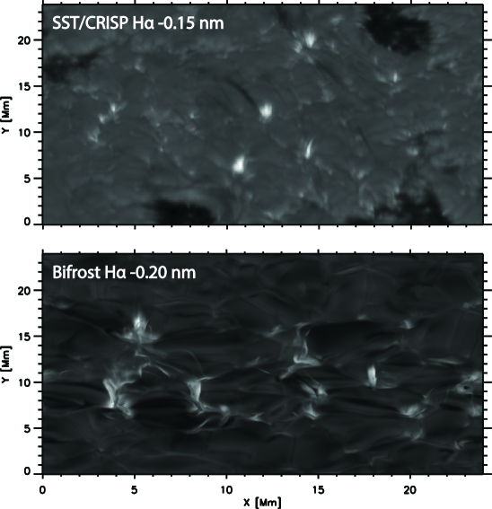
Figure 1.— Simulated H$\alpha$ line wing emission in EBs closely resembles flame like structures seen in high resolution ground based observations. H$\alpha$ intensity in the blue wing (at $-150$ pm) observed with SST/CRISP (top) and at $-200$ pm in the synthetic Bifrost images (bottom), at a solar heliocentric angle $\mu=0.5$. A version of this figure is available as an animation (Movie 1a), showing the variation of the flame like structures over a period of some 180 s. In addition an animation (Movie 1b) showing the time variation of the synthetic H$\alpha$ near the line core (at $+50$ pm) over the same time period is provided. Both animations are shown at heliocentric angle $\mu=0.5$.

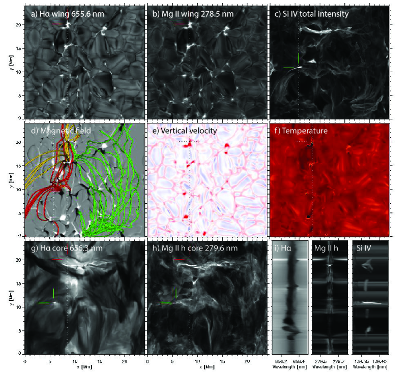
Figure 2.— Modeled spectra show signatures that resemble the characteristics of EBs, UV bursts and small flares. H$\alpha$ line wing (a), Mg II line wing (b), Si IV total intensity (c); photospheric magnetogram ($B_{z}$) and selected field lines (d), photospheric velocity $u_{z}$ (e) and temperature (f); H$\alpha$ line core (g), Mg II line core (h), and line profiles of H$\alpha$, Mg II along $x=8.5$, and Si IV along $x=6$ Mm (i). The red and green cross hairs show the location of a simulated EB and UV burst respectively. In panel d, yellow field lines have been traced from the EB site (indicated by the red orthogonal lines) and red field lines from the vicinity of the small flare. The green field lines have been traced from various magnetic polarities at $z=0$ Mm and for $x\geq 10$ Mm. An animation (Movie 2) of synthetic H$\alpha$ near the line core (at $+50$ pm) core seen from solar heliocentric angle of $\mu=1$ over a period of 200 s showing formation of opaque dark fibrils over the emerging flux region is provided.

2.1. Simulations

The numerical model described in this paper is produced by the Bifrost code (Gudiksen et al., 2011) which solves the magnetohydrodynamic equations on a 3D Cartesian grid. The modelled solar atmosphere spans from 2.5 Mm below the solar surface to 14 Mm above the photosphere, and fills 24$\times$24 Mm in the horizontal direction, i.e. the model covers the upper convection zone to the lower corona. A grid of $504\times 504\times 496$ was used with a uniform horizontal resolution of 48 km. The vertical resolution varies from 20 km/cell in the photosphere, chromosphere and transition region to nearly 100 km/cell in the corona and deeper convective layers, where the scale height is much larger. Optically thick radiative transfer and radiative losses from the photosphere and lower chromosphere, including scattering, are implemented using a short characteristics scheme (Hayek et al., 2010). Above the lower chromosphere, radiative losses are parameterized using recipes derived by 1D non-LTE radiative hydrodynamic simulations (Carlsson & Leenaarts, 2012) . Field aligned thermal conduction is included with the magnetohydrodynamic equations through operator splitting; the thermal conduction operator is solved using an implicit multi-grid method to allow a reasonably long time-step.

The model is initialized with a weak uniform oblique magnetic field ($<0.1$ G) that fills the corona, making an inclination angle of 45 degrees with respect to the $z$-axis. This field is sufficiently weak that it has no effect on the dynamics of the coronal plasma, but its non-vertical direction slows the conductive cooling. The coronal temperature is some 400 kK at the time of flux emergence, overlying a cool chromosphere mainly heated by acoustic shocks (see Ortiz et al., 2014, for further details). At the start of the numerical experiment, a steady state convective equilibrium has been achieved, the chromosphere is in a quasi steady state, while the corona is slowly cooling. Then, a non-twisted horizontal flux sheet of strength $3360$ G is injected at the bottom boundary. The magnetic sheet is oriented in the $y$ direction filling the area $[x;y]=[3-16;0-24]$ Mm, for a time period of 1 h 45 m (this is the same model as used in Archontis & Hansteen, 2014; Ortiz et al., 2014).

Initially, the magnetic field emerges to the photosphere, where it stops, since the field is no longer carried by convective motions nor is buoyant. As field ‘piles up’ from below, the magnetic pressure increases and in certain locations plasma-$\beta$ of the emerging field becomes smaller than one. In these locations magnetic flux elements can emerge through the photosphere and rise into the outer atmosphere above. These rising elements expand and rapidly penetrate and fill the chromosphere and corona, pushing the pre-existing ambient corona aside. The heating events that are described in this paper occur well after (some few thousand seconds) the flux sheet first encounters the photosphere and are a result of self interactions between the various magnetic elements that have pierced the photosphere and are spreading into the chromosphere and corona.

2.2. Diagnostics

The response of the solar atmosphere to the emergence and interactions of the rising magnetic field is studied by computing a number of spectral lines formed in the photosphere and corona.

Synthetic H$\alpha$ spectra were calculated in 3D non-LTE using the Multi3d code (Leenaarts & Carlsson, 2009). We used a five-level plus continuum hydrogen model atom and modeled the Ly$\alpha$ and Ly$\beta$ lines using complete redistribution (CRD) with a Gaussian profile with Doppler broadening only (Leenaarts et al., 2012a), as an approximation to the more time consuming partial redistribution (PRD) calculations. Radiative transfer calculations were carried out for a total of 24 angles, using the A4 set (Carlson, 1963). In addition to the snapshot calculated for display in Figures 1–4, we have calculated H$\alpha$ emission for a number of snapshots covering a period of 180 s in order to give an indication of the time evolution line. For these animations (Movies 1 and 2) the calculations were run with reduced horizontal spatial resolution (every second grid point) to reduce the computational burden. For some snapshots the vertical grid was interpolated to a finer scale to improve convergence times. Both of these procedures were found to have a negligible effect on the line profiles.

The Mg II synthetic spectra in the vicinity of the h&k lines were calculated in 1.5D non-LTE with PRD using the RH 1.5D code (Uitenbroek, 2001; Pereira & Uitenbroek, 2015). In 1.5D each vertical column from the simulation is treated as an independent 1D atmosphere. This allows for much faster calculations, at the expense of less realistic intensities for wavelengths close to the line cores. This approach is a good approximation for the greater part of the h&k line profiles (Leenaarts et al., 2013a), making the computations more tractable than the full 3D PRD calculations (Sukhorukov & Leenaarts, 2016). We used a 10-level plus continuum Mg II atom (Leenaarts et al. 2013b, same setup as Pereira et al. 2013, although additional lines of other elements were not included) and a hybrid angle-dependent PRD (Leenaarts et al., 2012b).

The Si IV 139.3744 nm line profiles were also calculated with the RH 1.5D code using a 9 level model atom including 5 levels of Si III, three levels of Si IV and the ground state of Si V. The overlapping Ni II line was included simultaneously using a four level model atom including the ground term of Ni II as two levels, the upper level of the Ni II 139.3324 nm line (93 km s^-1on the blue side of the Si IV line core) and the ground term of Ni III. The background continuum of Si I was also included in non-LTE employing a 16 level model atom with 15 levels of Si I and the ground state of Si II.

2.3. Observations

In order to compare and contrast our synthetic spectra with equivalent observational spectra we show observations obtained at the Swedish 1-meter Solar Telescope (Scharmer et al., 2003) using the CRISP instrument (Scharmer et al., 2008) on September 27 2015 at 10:00:39 UT, centered on the emerging active region NOAA 12423. For exploration of the multi-dimensional simulation and observational data cubes, we made much use of CRISPEX (Vissers & Rouppe van der Voort, 2012).

CRISP was running a 3-line program at a temporal cadence of 32 s during which the H$\alpha$ spectral line was sampled at 15 line positions between $\pm 150$ pm. The CRISP program further includes spectral sampling of the Fe I 617.3 nm and Ca II 854.2 nm lines. CRISP data were processed following the CRISPRED data reduction pipeline (de la Cruz Rodríguez et al., 2015), which includes Multi-Object Multi-Frame Blind Deconvolution image restoration (van Noort et al., 2005). The spatial sampling is 0.057 arcsec per pixel, the diffraction limit at 656.3 nm is 0.14 arcsec. The complete time series has a duration of 02:43 hours, from 07:47 to 10:30 UT.

Simultaneous data was obtained with NASA’s Interface Region Imaging Spectrograph (IRIS, De Pontieu et al., 2014) which was observing the same active region running an observing program labeled OBS-ID 3620106168. This program comprises a medium-dense 128-step raster with continuous 0.33 arcsec steps of the 60 arcsec spectrograph slit covering a spatial area of 42.2 arcsec$\times$ 60 arcsec at a temporal cadence of 10:53 min. The exposure time was 4 s. To increase signal-to-noise the IRIS spatial sampling was summed on board ($2\times 2$ pixel binning) so that the original IRIS resolution of 0.166 arcsec spatial sampling was reduced to 0.33 arcsec spatial sampling while the spectral sampling was reduced from $3$ km s^-1to $6$ km s^-1sampling. The IRIS data were calibrated to “level 2”, i.e., including dark current, flat-field and geometric correction (De Pontieu et al., 2014). The slit-jaw images (SJI) were corrected for dark-current and flat-field, as well as internal co-alignment drifts.

Alignment between the SST and IRIS data was done through cross-correlation of CRISP Ca II 854.2 nm wing images and IRIS 279.6 nm slit jaw images.

3. Results

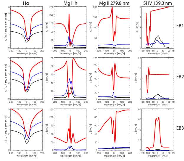
Figure 3.— Synthetic line profiles from 3 selected Ellerman bombs, as seen from straight above, showing H$\alpha$ (first column), the Mg II h line, Mg II triplet lines (middle columns) and Si IV 139.3744 nm (fourth column) including Ni II 139.3324 nm line located 93 km s^-1blue-wards of the Si IV line center. Each row represents a different event. The red line shows the EB spectra, the black lines show the average profiles of the entire simulation snapshot, while the blue lines show average spectra in the vicinity of the EB.

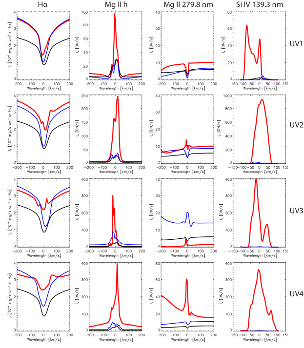
Figure 4.— Synthetic line profiles from 4 selected UV bursts, as seen from straight above, showing H$\alpha$ (first column), the Mg II h line, Mg II triplet lines (middle columns) and Si IV 139.3744 nm (fourth column) including Ni II 139.3324 nm line located 93 km s^-1blue-wards of the Si IV line center. Each row represents a different event. The red line shows the UV burst spectra, the black lines show the average profiles of the entire simulation snap shot, while the blue lines show average spectra in the vicinity of the UV burst.

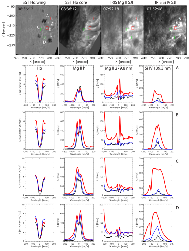
Figure 5.— SST and IRIS observations of 2 Ellerman bombs and 2 UV bursts seen at at a solar heliocentric angle $\mu=0.5$. The top panels show the H$\alpha$ line wing and core respectively (left images), as well as the Mg II k line and Si IV 1400 slit jaw images (right column). The lower panel rows show selected Ellerman bomb and UV burst, from locations A-D indicated in the top row, showing H$\alpha$ (first column) the Mg II h and Mg II triplet lines (middle columns) and Si IV 139.3744 nm, including Ni II 139.3324 line located 93 km s^-1blue-wards of the Si IV line center (right columns). The spectra A and B are Ellerman bombs, C and D UV bursts. The red line shows the EB or UV burst spectra, the black lines show the average profiles of the region surrounding the UV burst or EB, while the blue lines show time averaged spectra in the vicinity of the EB or UV burst.

A defining observed characteristic of EBs (Watanabe et al., 2011) is the appearance of rapidly varying extended flames, or jets, jutting out from the photospheric network in the H$\alpha$ line, most easily seen when looking off disk center (see Figure 1a). These synthetic observations can also be compared with observations obtained at the Swedish 1-meter Solar Telescope (Figure 1b). It is likely that these flames exist below a ‘canopy’ of dense chromospheric plasma, which prevents any hot emission from the photosphere to be visible in the H$\alpha$ line core, formed some $2000$ km above the photosphere (Leenaarts et al., 2012a). Thus, EBs appear far from line center on both sides of H$\alpha$ line center. Ellerman (1917) reported that the enhanced brightness extends at least 0.4-0.5 nm, and in certain cases attains a width of 3 nm. In the simulations (Figure 1a), synthetic images made in the far blue and red wings of H$\alpha$ show several EBs that are rooted in the photospheric network, located in intergranular lanes between opposite magnetic polarities. They all possess bright strands of dense plasma, which are vertically oriented, and they impart an overall flame-like structure to the EBs. These results come into close agreement with the location, morphology and dynamics of observed EBs (see also Movie 1a and 1b which show the time evolution in the line wing and at $+50$ pm from the line core).

Synthetic spectroheliograms from the model (Figure 2a, 2b) show that EBs appear as small (size $1-1.5$ Mm) bright structures in the far wings of H$\alpha$ and the Mg II h&k lines. They occur at the interface between opposite polarity fields of adjacent emerging bipoles (Figure 2d). Profound downflows (Figure 2e) occur on either side of the interface, due to plasma draining along the flanks of the emerging bipoles. The plasma at photospheric heights in the interface is heated to $8-9\times 10^{3}$ K (Figure 2f), giving onset to EBs.

The synthetic EBs are not visible at the line core of the H$\alpha$ and Mg II h lines (Figure 2g, 2h) and they are barely visible in the Si IV 139.3 nm band (Figure 2c). Just as the H$\alpha$ core, the line core of the Mg II h&k lines are also mainly formed in the high chromosphere (Leenaarts et al., 2013a). Emission in the Si IV 139.3 nm line requires temperatures of at least $2\times 10^{4}$ K in the dense photosphere or $6-8\times 10^{4}$ K in the less dense corona where the coronal approximation is valid. Thus, they are not responsive to the EBs generated here, which remain below $<10^{4}$ K at photospheric heights. In the far wings of Mg II lines, and at the continuum near the Si IV line, (Figure 2i) lessening opacity allows brightening from the EBs to become visible through the overlying canopy, forming a bright ‘moustache’ (see also Figure 3).

On the other hand, the H$\alpha$ line core (Figure 2g) reveals the existence of extended ‘dark’ loops (e.g. at $x=14$ Mm, $y=0-14$ Mm, see also Movie 2 which shows the time evolution in H$\alpha$ at $+50$ pm as seen from above), which are lying along the overarching field-lines (e.g. green field-lines in Figure 2d) that connect distant opposite polarities in the emerging flux region. These newly formed loops carry cool and dense plasma from the photosphere/chromosphere and they may account for H$\alpha$ arch-filament systems.

At other locations, there is strong emission at Si IV, with no obvious corresponding signal in H$\alpha$ (core or wing) and only weak enhancement in Mg II. For instance, the Si IV signal for the brightening at $[x,y]=[8.5,12]$ Mm (Figure 2c, 2i) is 200 times stronger than the average while showing no obvious brightening in H$\alpha$ nor the Mg II h line. The absolute intensity of this brightening is of the same order of magnitude as hot explosions discovered by IRIS (e.g. Peter et al., 2014, see also Figure 5). The Si IV line profile is also very broad in this location, as discussed below, and thus, these events may correspond to the observed UV bursts.

Moreover, there are brightenings with very strong emission at Si IV and considerable emission at the line core of H$\alpha$ and Mg II h line (e.g. at the location indicated by the green orthogonal lines, Figure 2c, 2g, 2h). This is where plasma at the upper chromosphere is heated to high temperatures $O(10^{6})$ K. These explosions are associated with the onset of small flares (Figure 6, 7).

3.1. Detailed spectra

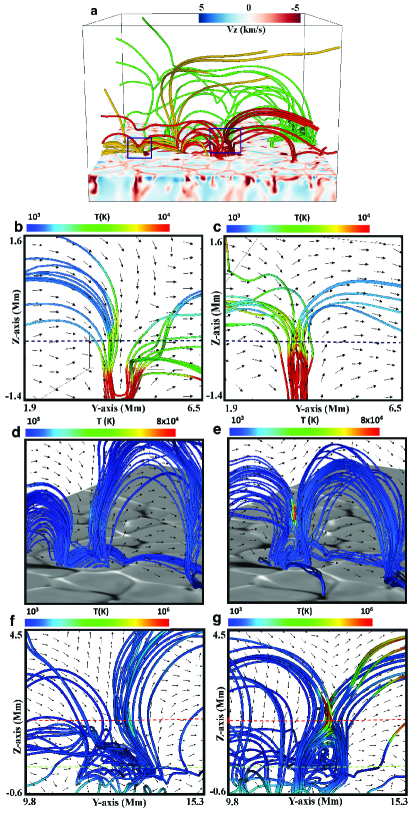
Figure 6.— Overall field-line topology and the onset of an EB, UV burst and a small chromospheric flare. a, Selected field-lines showing the serpentine field at $t=9160$ s. Yellow and red field-lines have been traced from the areas highlighted by the black insets (left and right respectively). The image shows the distribution of vertical velocity at the photosphere (red color indicates downflowing material). b-c, Close-up of the field-lines, which have been traced from within the left inset in (a), at $t=8800$ s (b) and $t=9160$ s (c). They are colored according to the value of the temperature. The arrows show the projection of the full magnetic field vector at $x=8.4$ Mm. The horizontal (dashed) line shows the photosphere. The localized temperature enhancement, just above $z=0$ Mm and $y\approx 3.5$ Mm, illustrates the location of the EB. d-e, Emergence of $\Omega$-loops, out of the serpentine field-lines (d, $t=7870$ s), leads to expansion and reconnection at the chromosphere (e, $t=7930$ s) and the triggering of a UV burst. The downward-released reconnected field-lines, build an arcade anchored in the photosphere. The chromospheric plasma at and close to the reconnection site (e.g. at the top of the arcade, $y=4.7$ Mm, $z=1.3$ Mm) is heated to high temperatures, triggering a UV burst. The horizontal slice shows the $B_{z}$ distribution at the photosphere (white (black) shows positive (negative) $B_{z}$, in the range $[-10^{3},10^{3}$ G]). The arrows show the full magnetic field vector at $x\approx 8$ Mm. f-g, Close-up of the field-lines, which have been traced from within the right inset in (a), at $t=8800$ s (f) and $t=9250$ s (g). The arrows show the projection of the full magnetic field vector at $x\approx 6$ Mm. The two horizontal (dashed) lines show heights at $z=1.75$ Mm and at $z=0$ Mm. Nearby emerging loops come into contact and reconnect in a similar manner to the UV burst case. Energy release occurs at the upper chromosphere (around $z=1.8$ Mm, $y=13$ Mm), where plasma is less dense, leading to profound plasma heating ($10^{6}$ K) and the onset of a small chromospheric flare.

The observational signatures of EBs and UV bursts are quite complicated. To give further insight we here present several synthetic line spectra from reconnection events occurring in the photosphere and in the middle to upper chromosphere and compare them with observed spectra taken at the SST and with IRIS.

In addition to the ‘flamelike’ structure seen in the wings of H$\alpha$ a number of ‘secondary’ EB characteristics have been reported (Vissers et al., 2015). In Figure 3, we present the spectra of several simulated EBs in H$\alpha$, the Mg II h line near 279.6 nm, the Mg II triplet lines near 279.8 nm and the Si IV 139.3744 nm line (including the Ni II blend at 139.3324 nm). In Figure 4 the spectra of synthetic UV-bursts are shown.

Figure 3 shows that the H$\alpha$ line core is unaffected by the presence of the EB, mainly due to the existence of an overlying chromospheric canopy above the EB. For all cases, we find that the line wings are significantly enhanced; by roughly a factor two when seen from directly above, and that this enhancement extends sοme 0.1 nm or more on either side of the line core. As for H$\alpha$, the Mg II line core is opaque and emission in the core largely stems from the overlying (usually cooler) chromosphere, but the overlying material becomes transparent as one moves away from the central core and we see brightenings, sometimes asymmetric, in the outer core and wings of the Mg II h line, as well as large brightening in the continuum surrounding the line.

In most of the simulated EBs, we also find asymmetric emission in the Mg II triplet lines near 279.8 nm. Emission in these lines is observationally rare and indicates that the chromospheric temperature is high at low chromospheric heights (Pereira et al., 2015).

In general, we do not find any significant enhancement in the Si IV 139.3744 nm line above our simulated EBs. In the cases that we have studied, we usually find enhanced continuum emission and absorption in the Ni II line (which sometimes shows a complicated line structure indicative of large relative flows in the chromosphere). In some instances we find enhanced Si IV emission in the same locations as the EB, but these are often dominated by heating events, unrelated to the EB, at greater heights in the chromosphere. Though the emission is unrelated, the magnetic field structure of these brightenings is connected, forming active sites in the larger magnetic flux structure that is emerging through the photosphere. This possible connection between disparate emitting sites has also been noted observationally (Qiu et al., 2000). Note that when seen from the side we occasionally see that the upper part of the EB does produce emission in Si IV, but in every instance we have found this is dominated by emission from greater heights when seen from above.

Simulated line profiles from reconnection events that occur higher in the atmosphere are shown in Figure 4. The H$\alpha$ core emission from these events depends on event height and strength, while the wing emission is always unresponsive. The line core can either be unresponsive, or in some cases show significant brightening and complex structure for the strongest most violent events — perhaps forming a counterpart to small flares.

The Mg II h line core emission is enhanced by a large factor and the core line profile shows quite complicated structure reflecting the high velocity jets that form the core of these reconnection events. As for H${\alpha}$, the Mg II triplet line emission does not always respond to these UV-bursts, but occasionally show asymmetric emission profiles and emission.

On the other hand, the Si IV emission is greatly enhanced in some cases. It can increase as much as three orders of magnitude over the average value and it reflects intensities comparable to those measured with IRIS. The line profile of the Si IV lines is quite complex, but in general shows bi-directional Doppler shifts with amplitudes up to 100 km s^-1. The Si IV line profile is very broad, of order 100 km s^-1, indicating highly supersonic velocities for the lines formed at the greatest heights (the speed of sound is of order 30 km s^-1 at the temperature of Si IV emission). The cases of high Si IV intensities we report here are all formed in the middle to upper chromosphere and we find that the line has moderate opacity, with $\tau\sim 10$. We would expect Si IV to be even thicker, were the line formed deeper in the atmosphere, e.g. in connection with an EB.

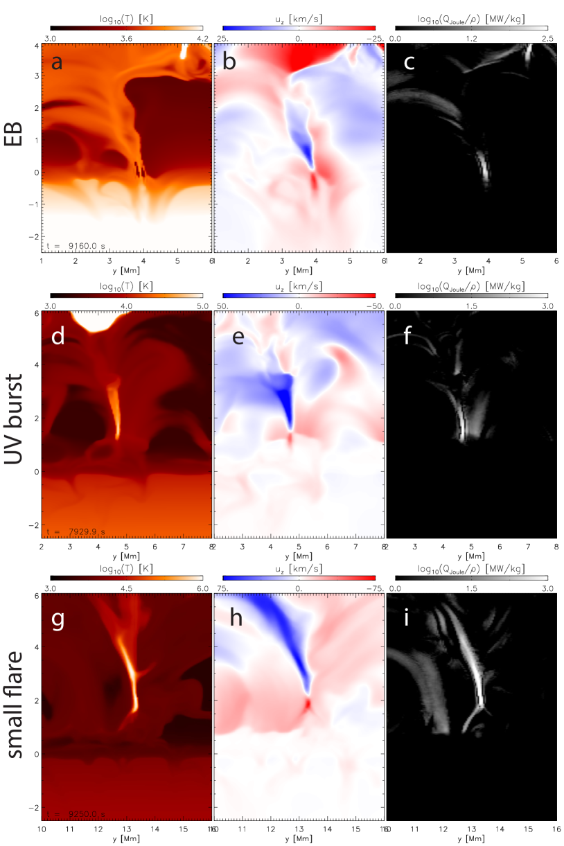
Figure 7.— Reconnection in the photosphere and chromosphere heats the local plasma and give rise to fast (supersonic) bi-directional jets at several heights. 2D cuts at $x=8.43$ Mm, $t=9160$ s (a-c), $x=8.05$ Mm, $t=7930$ s (d-f) and $x=6.14$ Mm, $t=9250$ s (g-i). Shown is: temperature (first column), vertical velocity (second column), Joule dissipation over density (third column). A version of this figure is available as an animation (Movie 3) showing the time development of these variable over a period of 500 s.

To make a comparison between the simulated spectra and the observations, we present line profiles of a number of EBs and UV bursts observed with the SST and IRIS on September 27 2015 starting at 07:52:39 UT in the vicinity of active region NOAA 12423. Two sets of two spectra are presented in Figure 5.

In the first two cases, (A) and (B), two Ellerman bombs were selected by inspecting the H$\alpha$ wing spectroheliogram for bright flamelike structures and then plotting the spectra of H$\alpha$ and the concurrent IRIS UV lines in the same region. In addition, to give an idea of the temporal variability of these lines in that region, we plot the average profile and spectra at a temporal cadence of some 22 minutes for the entire observational run lasting some 4.5 hours. H$\alpha$ responds as expected, with bright wings and unresponsive core emission. The Mg II h line core emission is unresponsive, while the h2 peaks are broadened, sometimes (case B), showing increased emission, as is also the case in the continuum where the intensity increases by almost a factor 2. The Mg II triplet lines show both enhanced emission and asymmetric profiles. In the Si IV line we find broad $O(200\mathrm{km~{}s}^{-1})$ profiles and enhanced emission, but less than in the UV burst cases discussed below.

Likewise, cases (C) and (D) were selected by searching for bright Si IV SJI emission and then plotting H$\alpha$ and the other IRIS lines concurrently, including average and time variability spectra for reference. The Si IV line spectra are extremely broad $O(300\mathrm{km~{}s}^{-1})$, sometimes asymmetric (case D), and Ni II absorption is strong in both examples. H$\alpha$ emission, on the other hand, seems quite unresponsive. We note that there is a Ellerman bomb-like brightening that occurs in case D, but it appears some 66 minutes after the original Si IV brightening and is slightly offset from the Si IV SJ emission, thus likely not representing the same event. Mg II h line emission is enhanced, both in the h2 peaks and (case C) in the h3 line core, as well as being asymmetric. The continuum emission is slightly enhanced. The Mg II triplet lines are in emission, though to a much smaller extent than as seen in the EB cases (A and B).

The time cadence of this observation is unfortunately too low to show the time evolution of these events clearly, obtaining such data should be a goal for future studies.

3.2. Dynamics and energetics

To understand the mechanism for the onset of the EBs, UV bursts, and small flares in our experiment, we study the topology of the magnetic field (Figure 6a). Initially, the sub-photospheric magnetic field is pulled up by convective up-flows and buoyancy (where the field is strong) and it is dragged down by downdrafts, developing an undulating shape. When the strongest field breaks through the surface, small ($1-2$ Mm) magnetic bipoles appear at the photosphere. Eventually, the field expands into the ambient atmosphere forming $\Omega$-like loops, which may reconnect with each other, creating longer magnetic structures (i.e. the arch-filaments shown in Figure 2). As a result, the emerging magnetic field develops an overall “sea-serpent” configuration of loops with increasingly larger scale with height.

The EBs are formed at the photosphere, between the opposite polarity field-lines of adjacent emerging loops (Figure 6b, 6c). As the U-like parts of the undulating field are pulled down by convective down-flows, the nearby legs of the adjacent loops are pressed together and their field-lines reconnect, which leads to local plasma heating and the onset of EBs. A side effect of this process is the unloading of mass from the serpentine field (Isobe et al., 2007; Archontis & Hood, 2009; Cheung et al., 2010; Tortosa-Andreu & Moreno-Insertis, 2009). Reconnection above the density-loaded U-dips, forms twisted magnetic structures (O-shaped, as projected onto the $yz$-plane), which are dragged into the convection zone, together with their attached heavy plasma. Some amount of cool plasma is carried upward with the expanding field forming the opaque chromospheric canopy.

A similar mechanism occurs at larger heights, powering UV bursts (at $z\sim 1.5$ Mm, Figure 6d, 6e) and small flares (at $z\sim 1.8$ Mm, Figure 6f, 6g). The lateral expansion of adjacent $\Omega$-loops, brings their oppositely-directed stressed fields into contact, leading to reconnection at their interface and heating of chromospheric plasma to high temperatures ($7-8\times 10^{4}$ K for the UV bursts and $\sim 1$ MK for the small flares).

Figure 7 shows vertical cuts at the locations of an EB (a-c), UV burst (d-f) and small chromospheric flare (g-i). In all cases, strong currents are built up at the interfaces between the interacting magnetic fields. Reconnection at the current layers leads to plasma heating via Joule dissipation (c, f, i, Movie 3 which shows the time evolution of these quantities) and to the emission of bi-directional flows (b, e, h) with velocities comparable to the local Alfvén speed. Note that the velocities are asymmetric, with the upward propagating portion having substantially higher velocity (see e.g. Libbrecht et al., 2016). The afore mentioned events have lifetimes of at least 120-180 s.

Above the EB, dense ($\sim 10^{-8}$ g cm^-3) and cool ($\sim 7.5\times 10^{3}$ K) plasma is emitted along the reconnection jet with a velocity of $\sim 20$ km s^-1. Some $1300$ km higher, at the site of the UV burst, dense chromospheric material ($\sim 5\times 10^{-13}$ g cm^-3) is heated to $\sim 7.5\times 10^{4}$ K (d). Before the burst, the local (unperturbed) plasma has similar density but it is 10 times cooler. The total intensity computed in the Si IV line also shows that the UV burst occurs at chromospheric heights ($z=1-2$ Mm) in this case. The reconnection jets run with speeds $40-70$ km s^-1(e). The upward jet shoots cool ($1-2\times 10^{4}$ K) chromospheric plasma to coronal heights (reaches $z\geq 4$ Mm at 7980 s). The downward jet terminates at the apex of the post-reconnection arcade (at $z\sim 1$ Mm) where the plasma is heated by compression. Our results suggest that most UV bursts may originate from low/mid chromospheric plasma and are not necessarily photospheric as previously suggested (Peter et al., 2014).

When stronger magnetic fields ($50-100$ G) reconnect in the upper chromosphere (e.g. $z\sim 2.1$ Mm, panel g), the local plasma ($\sim 1-1.5\times 10^{-13}$ g cm^-3) is heated to even higher temperatures ($O(10^{6})$ K). The local plasma-$\beta$, within the volume ($\sim 700\times 500\times 1000$ km³) of the profound heating, is $\sim 0.02$, which explains the increase of temperature by a factor of $\sim 1/\beta$. The hot and dense reconnection jets are emitted upward (up to $z\sim 4$ Mm) and downward (to $\sim 1.5$ Mm) with maximum speeds of some $80$ km s^-1.

The energetics of our synthetic EBs, UV bursts, and small flares can be estimated as follows: The (average) magnetic field close to the EB described in the main text is $\sim 600$ G. The total magnetic energy stored in the EB’s volume ($\sim 500~{}\mathrm{km}\times 500~{}\mathrm{km}\times 400~{}\mathrm{km})$ is $\sim 1.5\times 10^{20}$ J. The total thermal energy content is $\sim 10^{20}$ J. These values lie within the expected energy range for EBs. The magnetic field strength near the UV burst is $15-20$ G and plasma $\beta\approx 0.1$. Thus, the total magnetic energy dumped in the burst’s volume ($\sim 700~{}\mathrm{km}\times 500~{}\mathrm{km}\times 800~{}\mathrm{km}$) and the involved thermal energy are up to $3.8\times 10^{17}$ J and $2-3\times 10^{17}$ J respectively, which are much less than those computed for the synthetic EB.

In the upper chromosphere, the flaring event described in the main text has a magnetic field of $50-100$ G. The total stored energy is $O(10^{18})$ J, which lies within the nanoflare energy regime. According to the above values, the heated plasma around the reconnection site may account for an EUV flare and the emitted jet for an EUV jet.

4. Discussion and Conclusions

The simulations and synthetic diagnostics presented here show that many, though perhaps not all, observed characteristics of Ellerman bombs and UV bursts can be reproduced within the confines of a relatively simple scenario where a untwisted flux sheet is allowed to emerge through the solar atmosphere and expand into the overlying atmosphere.

While H$\alpha$ and the Mg II triplet lines appear very similar to the observed spectra presented in Fig 5, the Mg II h (and k) lines are not as easy to characterize. The observed EB spectra show enhanced h2 and slightly enhanced h3 peaks and line wings. The synthetic spectra show strongly enhanced wings but only sometimes enhanced cores and strong asymmetries. We suspect that the difference in viewing angle ($\mu=1$ for the simulations, $\mu=0.5$ for the observations) is the cause of the difference in the wings: Grubecka et al. (2016) observe EBs close to disk center and they observe strongly enhanced wings. The observed UV burst spectra show strong enhancement for the h2 cores, sometimes enhanced h3 and intensity increases in the continuum. This is not too different from what is found in the synthetic spectra, though the increase in core width is much greater in many observed spectra. It should be noted that the variations in Mg II h&k line response to UV bursts is very large as can be ascertained also from other sources (Grubecka et al., 2016; Vissers et al., 2015).

The synthetic Si IV spectra show an intriguing similarity to the observed line profiles, but there are also differences that could point the way towards a better understanding of the solar atmosphere in general and EBs and UV bursts in particular. We found no Ni II absorption in those Si IV line profiles that extend to more than 100 km s^-1in the blue. This could be due to several factors: 1) there is not enough cool material above the sites of strong Si IV emission in the model to give sufficient opacity in the Ni II line, 2) the simulated EBs and deep UV bursts do not heat the denser low atmosphere material to high enough temperatures to cause Si IV emission and/or 3) the velocities in deeper UV bursts are not great enough to give significant emission at a blue-shift of 100 km s^-1in locations where the opacity of the overlying material is great enough. We note that reconnection in this model is mediated by the use of an artificial hyper-diffusive operator, necessary to prevent the collapse of current sheets to smaller widths than the grid size (48 km). The effective diffusivity on the real Sun may allow current sheets to become thinner, with attendant higher temperatures. Not covered in this study is the possibility that reconnection, even at low heights in the atmosphere, produces non-thermal electrons in sufficient quantities to perturb emission. Ding et al. (1998) and Fang et al. (2006) show that this process may be of interest. In particular these authors find that the the temperature rise needed to explain EB emission is somewhat lower than that found in models without particle beams. On the other hand it is also likely that since EBs have a fairly large vertical extent, also with respect to Joule heating (see Figure 7), a slightly altered magnetic topology could lead to Si IV emission from the upper part of EBs rooted in the photosphere, even in models with relatively poor resolution, such as this one. The study of EBs and UV bursts, by comparing observational and synthetic diagnostics, thus presents a unique opportunity to study reconnection, and the physical parameters controlling reconnection, at many heights in the solar atmosphere.

In order to form the coronal magnetic field, emerging magnetic flux must break through the photosphere, while ridding itself of considerable mass. This process needs reconnection in order to proceed, occurring at several heights as the field rises into the upper atmosphere forming continually longer loops. The above results reveal that reconnection between stressed magnetic fields in an emerging flux region can trigger three types of solar explosive events (EBs, UV bursts, and small chromospheric flares) of different origins. We conjecture that a similar mechanism can form a continuum of explosions across the solar atmosphere, depending on the local properties of the plasma and the amount of available energy involved in the process whose visibility is determined by the amount of overlying opaque (and cool) material.

References

- Archontis & Hansteen (2014) Archontis, V. & Hansteen, V. 2014, ApJ, 788, L2
- Archontis & Hood (2009) Archontis, V. & Hood, A. W. 2009, A&A, 508, 1469
- Babcock (1963) Babcock, H. W. 1963, ARA&A, 1, 41
- Berlicki & Heinzel (2014) Berlicki, A. & Heinzel, P. 2014, A&A, 567, A110
- Carlson (1963) Carlson, B. G. 1963, Methods in Computational Physics, ed. B. Alder, S. Fernbach, & M. Rotenberg, Vol. 1 (New York: Academic)
- Carlsson & Leenaarts (2012) Carlsson, M. & Leenaarts, J. 2012, A&A, 539, A39
- Cheung et al. (2010) Cheung, M. C. M., Rempel, M., Title, A. M., & Schüssler, M. 2010, ApJ, 720, 233
- Danilovic (2017) Danilovic, S. 2017, ArXiv e-prints [\eprint[arXiv]1701.02112]
- de la Cruz Rodríguez et al. (2015) de la Cruz Rodríguez, J., Löfdahl, M. G., Sütterlin, P., Hillberg, T., & Rouppe van der Voort, L. 2015, A&A, 573, A40
- De Pontieu et al. (2014) De Pontieu, B., Title, A. M., Lemen, J. R., et al. 2014, Sol. Phys., 289, 2733
- Ding et al. (1998) Ding, M. D., Henoux, J.-C., & Fang, C. 1998, A&A, 332, 761
- Ellerman (1917) Ellerman, F. 1917, ApJ, 46, 298
- Fang et al. (2006) Fang, C., Tang, Y. H., Xu, Z., Ding, M. D., & Chen, P. F. 2006, ApJ, 643, 1325
- Georgoulis et al. (2002) Georgoulis, M. K., Rust, D. M., Bernasconi, P. N., & Schmieder, B. 2002, ApJ, 575, 506
- Grubecka et al. (2016) Grubecka, M., Schmieder, B., Berlicki, A., et al. 2016, A&A, 593, A32
- Gudiksen et al. (2011) Gudiksen, B. V., Carlsson, M., Hansteen, V. H., & et al. 2011, A&A, 531, A154
- Hayek et al. (2010) Hayek, W., Asplund, M., Carlsson, M., et al. 2010, A&A, 517, A49
- Hong et al. (2014) Hong, J., Ding, M. D., Li, Y., Fang, C., & Cao, W. 2014, ApJ, 792, 13
- Isobe et al. (2007) Isobe, H., Tripathi, D., & Archontis, V. 2007, ApJ, 657, L53
- Leenaarts & Carlsson (2009) Leenaarts, J. & Carlsson, M. 2009, in Astronomical Society of the Pacific Conference Series, Vol. 415, The Second Hinode Science Meeting: Beyond Discovery-Toward Understanding, ed. B. Lites, M. Cheung, T. Magara, J. Mariska, & K. Reeves, 87
- Leenaarts et al. (2012a) Leenaarts, J., Carlsson, M., & Rouppe van der Voort, L. 2012a, ApJ, 749, 136
- Leenaarts et al. (2012b) Leenaarts, J., Pereira, T., & Uitenbroek, H. 2012b, A&A, 543, A109
- Leenaarts et al. (2013a) Leenaarts, J., Pereira, T. M. D., Carlsson, M., Uitenbroek, H., & De Pontieu, B. 2013a, ApJ, 772, 89
- Leenaarts et al. (2013b) Leenaarts, J., Pereira, T. M. D., Carlsson, M., Uitenbroek, H., & De Pontieu, B. 2013b, ApJ, 772, 90
- Libbrecht et al. (2016) Libbrecht, T., Joshi, J., de la Cruz Rodríguez, J., Leenaarts, J., & Asensio Ramos, A. 2016, ArXiv e-prints [\eprint[arXiv]1610.01321]
- Matsumoto et al. (2008) Matsumoto, T., Kitai, R., Shibata, K., et al. 2008, PASJ, 60, 577
- Ni et al. (2016) Ni, L., Lin, J., Roussev, I. I., & Schmieder, B. 2016, ApJ, 832, 195
- Ortiz et al. (2014) Ortiz, A., Bellot Rubio, L. R., Hansteen, V. H., de la Cruz Rodríguez, J., & Rouppe van der Voort, L. 2014, ApJ, 781, 126
- Pariat et al. (2004) Pariat, E., Aulanier, G., Schmieder, B., et al. 2004, ApJ, 614, 1099
- Parker (1955) Parker, E. N. 1955, ApJ, 122, 293
- Pereira et al. (2015) Pereira, T. M. D., Carlsson, M., De Pontieu, B., & Hansteen, V. 2015, ApJ, 806, 14
- Pereira et al. (2013) Pereira, T. M. D., Leenaarts, J., De Pontieu, B., Carlsson, M., & Uitenbroek, H. 2013, ApJ, 778, 143
- Pereira & Uitenbroek (2015) Pereira, T. M. D. & Uitenbroek, H. 2015, A&A, 574, A3
- Peter et al. (2014) Peter, H., Tian, H., Curdt, W., et al. 2014, Science, 346, C315
- Qiu et al. (2000) Qiu, J., Ding, M. D., Wang, H., Denker, C., & Goode, P. R. 2000, ApJ, 544, L157
- Reid et al. (2016) Reid, A., Mathioudakis, M., Doyle, J. G., et al. 2016, ApJ, 823, 110
- Rouppe van der Voort et al. (2016) Rouppe van der Voort, L. H. M., Rutten, R. J., & Vissers, G. J. M. 2016, A&A, 592, A100
- Rutten et al. (2013) Rutten, R. J., Vissers, G. J. M., Rouppe van der Voort, L. H. M., Sütterlin, P., & Vitas, N. 2013, Journal of Physics Conference Series, 440, 012007
- Scharmer et al. (2003) Scharmer, G. B., Bjelksjo, K., Korhonen, T. K., Lindberg, B., & Petterson, B. 2003, in Society of Photo-Optical Instrumentation Engineers (SPIE) Conference Series, Vol. 4853, Innovative Telescopes and Instrumentation for Solar Astrophysics, ed. S. L. Keil & S. V. Avakyan, 341–350
- Scharmer et al. (2008) Scharmer, G. B., Narayan, G., Hillberg, T., et al. 2008, ApJ, 689, L69
- Sukhorukov & Leenaarts (2016) Sukhorukov, A. V. & Leenaarts, J. 2016, ArXiv e-prints [\eprint[arXiv]1606.05180]
- Tian et al. (2016) Tian, H., Xu, Z., He, J., & Madsen, C. 2016, ApJ, 824, 96
- Tortosa-Andreu & Moreno-Insertis (2009) Tortosa-Andreu, A. & Moreno-Insertis, F. 2009, A&A, 507, 949
- Uitenbroek (2001) Uitenbroek, H. 2001, ApJ, 557, 389
- van Noort et al. (2005) van Noort, M., Rouppe van der Voort, L., & Löfdahl, M. G. 2005, Sol. Phys., 228, 191
- Vissers & Rouppe van der Voort (2012) Vissers, G. & Rouppe van der Voort, L. 2012, ApJ, 750, 22
- Vissers et al. (2013) Vissers, G. J. M., Rouppe van der Voort, L. H. M., & Rutten, R. J. 2013, ApJ, 774, 32
- Vissers et al. (2015) Vissers, G. J. M., Rouppe van der Voort, L. H. M., Rutten, R. J., Carlsson, M., & De Pontieu, B. 2015, ApJ, 812, 11
- Watanabe et al. (2011) Watanabe, H., Vissers, G., Kitai, R., Rouppe van der Voort, L., & Rutten, R. J. 2011, ApJ, 736, 71
- Xu et al. (2011) Xu, X.-Y., Fang, C., Ding, M.-D., & Gao, D.-H. 2011, Research in Astronomy and Astrophysics, 11, 225