UWThPh-2017-08

Marcus Sperling and Harold C. Steinacker

Faculty of Physics, University of Vienna
Boltzmanngasse 5, A-1090 Vienna, Austria

Abstract

We study in detail generalized 4-dimensional fuzzy spheres with twisted extra dimensions. These spheres can be viewed as $SO(5)$-equivariant projections of quantized coadjoint orbits of $SO(6)$. We show that they arise as solutions in Yang-Mills matrix models, which naturally leads to higher-spin gauge theories on $S^{4}$. Several types of embeddings in matrix models are found, including one with self-intersecting fuzzy extra dimensions $S^{4}\times{\cal K}$, which is expected to entail 2+1 generations.

1 Introduction

The purpose of this paper is to present in detail a new class of covariant 4-dimensional quantum spheres ${\cal S}^{4}_{\Lambda}$, and to show that they arise as solutions of Yang-Mills-type matrix models. The results in this paper should provide the basis for studying physical applications, in particular for the higher spin theories arising on such spaces, which were argued to contain gravity [1, 2].

The long-term motivation for this work is to find an appropriate framework for quantum geometry which accommodates both gravity and quantum mechanics. Among the many attempts towards this goal, one strategy is to use some sort of non-commutative geometry, in order to avoid point-like singularities. However, several problems arise in that context. One issue is to ensure (local) Lorentz invariance, which must hold with high precision. Another issue is known as UV/IR mixing, which is a very generic phenomenon on non-commutative spaces that typically leads to unacceptably large non-local (and Lorentz-violating) effects [3, 4, 5, 6]. The latter problem is avoided in the maximally supersymmetric IKKT model, which was proposed as a constructive definition of IIB string theory [7].

To address the issue of Lorentz invariance, it seems useful to examine in more detail the few known examples of 4-dimensional quantum (or fuzzy) spaces which are compatible with the full classical rotational and translational symmetries. In the Euclidean case, the best-known example is the fuzzy 4-sphere ${\cal S}^{4}_{N}$ [8, 9, 10]. Taking this as a background in the IKKT model indeed leads to an interesting $SO(5)$-covariant higher-spin gauge theory [1], see also [2]. However some issues with the proper identification of the graviton suggest to consider certain generalized fuzzy 4-spheres, which were introduced in [1] and denoted as ${\cal S}^{4}_{\Lambda}$. These provide additional structure which may be relevant to particle physics and gravity. However, the internal structure of ${\cal S}^{4}_{\Lambda}$ is rather intricate and requires a detailed elaboration, which is provided in the present paper.

The most interesting feature of the generalized ${\cal S}^{4}_{\Lambda}$ is that they realize a compactified phase space (or tangent bundle) of a 4-sphere, supplemented by additional structure. They are in fact 10-dimensional bundles over $S^{4}$, which allows to naturally accommodate graviton modes as coefficients of momentum generators, as discussed in [1]. Additionally, the structure of ${\cal S}^{4}_{\Lambda}$ allows for novel types of embeddings in Yang-Mills matrix models, using either position generators, or momentum generators, or both. In the latter case, the fuzzy extra dimensions provide further structure and should justify the dimensional reduction to $S^{4}$. Finally, the momentum picture, as suggested in [20], can now be realized in a well-defined way via finite-dimensional matrices, which should allow to clarify the mechanism for gravity in this scenario.

The mathematical structure of the novel class of spaces is as follows: Fuzzy ${\cal S}^{4}_{\Lambda}$ is a quantization of a certain coadjoint orbit ${\cal O}_{\Lambda}$ of $SO(6)$, defined in terms of irreducible representations with highest weight $\Lambda$. The orbit ${\cal O}_{\Lambda}$ is a bundle over $S^{4}$ via some $SO(5)$-covariant projection, similar to a Hopf map. Since the underlying orbit ${\cal O}_{\Lambda}$ is 10-dimensional (or 6-dimensional for fuzzy ${\cal S}^{4}_{N}$), there is a 6-dimensional fiber, and ${\cal O}_{\Lambda}$ is a twisted (=equivariant) bundle over $S^{4}$. The “twisted” bundle structure means that the local stabilizer group $SO(4)$ of some point on $S^{4}$ acts non-trivially on the fiber. Consequently, fluctuations lead to a higher spin theory on $S^{4}$, in marked contrast to conventional Kaluza-Klein compactifications.

The accidental isomorphisms $\mathfrak{so}(6)\cong\mathfrak{su}(4)$ provides two useful and complementary views of ${\cal O}_{\Lambda}$: either as a $S^{4}\times S^{2}$ bundle over $S^{4}$ or as a ${\mathbb{C}}P^{2}$ bundle over ${\mathbb{C}}P^{3}$, which in turn is a $S^{2}$ bundle over $S^{4}$. The first picture is compatible with $SO(5)$, but some degeneracies are hidden, which are resolved in the second picture. In particular, we observe an interesting triple self-intersection (or covering) structure in the extra dimensions of ${\cal S}^{4}_{\Lambda}$, which is best understood in terms of the ${\mathbb{C}}P^{2}$ fiber. This is very similar to the squashed ${\mathbb{C}}P^{2}$ found as extra dimensions in [21, 22], and it strongly suggests 3 families of fermionic (near-)zero modes. In fact, one of these families would be distinct from the other two, which suggests a “2+1” family structure. This is a very intriguing albeit preliminary observation, and a further elaboration is postponed to future work.

The outline of this article is as follows: first, we briefly review the basic fuzzy 4-sphere in Section 2. Next, in order to describe the aforementioned structures of the generalized 4-sphere explicitly, we identify suitable matrix coordinates in the semi-classical case in Section 3. The semi-classical Poisson geometry then suggests the appropriate generators for the fuzzy case, and in Section 4 we work out the algebraic properties of these matrix observables. In particular, we show that the generalized ${\cal S}^{4}_{\Lambda}$ is indeed a solution of the Yang-Mills type matrix models such as the IKKT model, with a suitable potential term that is argued to arise at 1-loop. Apart from the obvious embedding via the Lie algebra generators, we find novel types of solutions in Section 5, which are interpreted as momentum and phase space embeddings. Moreover, in Section 6 we elaborate on the effective metric on these bundles arising from the different embeddings. Lastly, in Appendix A we provide more technical details of the fuzzy geometry.

The paper is intended as a technical resource for research involving the ${\cal S}^{4}_{\Lambda}$ spheres and similar spaces. The contents presented should provide all the necessary geometrical and algebraic tools for justifying, for example, dimensional reduction, and for extracting the low-energy physics on such a background. However, since we cannot determine the relevant scale parameters of the embeddings at this point, the physical perspectives of the resulting higher-spin theory are only briefly discussed here, and postponed to future work.

2 Covariant fuzzy four-spheres

We are interested in fuzzy 4-spheres which are covariant under $SO(5)$. They will be defined in terms of five hermitian matrices $X^{a},\ a=1,\ldots,5$ acting on some finite-dimensional Hilbert space ${\cal H}$, and transforming as vectors under $SO(5)$

$$[{\cal M}_{ab},X_{c}] =i(\delta_{ac}X_{b}-\delta_{bc}X_{a}),$$

$$[{\cal M}_{ab},{\cal M}_{cd}] =i(\delta_{ac}{\cal M}_{bd}-\delta_{ad}{\cal M}_{bc}-\delta_{bc}{\cal M}_{ad}+\delta_{bd}{\cal M}_{ac})\ .$$ (2.1)

Throughout this paper, indices are raised and lowered with $g_{ab}=\delta_{ab}$. The ${\cal M}_{ab}=-{\cal M}_{ba}$ for $a,b\in\{1,\ldots,5\}$ generate a suitable (not necessarily irreducible) representation of $\mathfrak{so}(5)$ on ${\cal H}$, and $X^{a}\in\mathrm{End}({\cal H})$ are operators interpreted as quantized embedding functions $X^{a}\sim x^{a}:\ S^{4}\hookrightarrow{\mathbb{R}}^{5}$. Then the radius

$$X^{a}X_{a} ={\cal R}^{2}$$ (2.2)

is a scalar operator of dimension $L^{2}$. We denote the commutator of the $X^{a}$ by

$$[X^{a},X^{b}] =:i\Theta^{ab}\ .$$ (2.3)

Such relations constitute a covariant quantum 4-sphere.

Particular realizations of such fuzzy 4-spheres are obtained from generators ${\cal M}^{ab},\ a,b=1,\ldots,6$ of $\mathfrak{so}(6)\cong\mathfrak{su}(4)$ via

$$X^{a} =r{\cal M}^{a6},\qquad a=1,\ldots,5\ ,\qquad\Theta^{ab}=r^{2}{\cal M}^{ab}\ .$$ (2.4)

Here $r$ is a scale parameter of dimension $L$, and ${\cal H}$ is some irreducible representation (irrep) of $\mathfrak{so}(6)$. In much of the paper we will set $r=1$ for simplicity. The $\mathfrak{so}(5)\subset\mathfrak{so}(6)$ subalgebra is recovered by restricting the indices of ${\cal M}^{ab}$ to $a,b=1,\ldots,5$.

This class of quantum spheres was considered in [1] as a promising basis for a higher-spin theory including gravity. Here we study their fuzzy geometry in more detail, and provide new embeddings in matrix models, which resolve some of the internal structure.

The covariant quantum 4-spheres can be viewed as compact versions of Snyder space [23, 24]. The crucial feature is that the classical isometry group (here $SO(5)$) is fully realized. This is in marked contrast to the basic quantum spaces such as the Moyal-Weyl quantum plane ${\mathbb{R}}^{4}_{\theta}$, where the Poisson tensor $\theta^{ab}$ breaks this symmetry. The price to pay is that the algebra of “coordinates” $X^{a}$ does not close, but involves extra generators $\Theta^{ab}$. Nevertheless, their proper geometric interpretation allows to proceed with the construction of physical theories on such spaces via matrix models, leading to fully covariant higher-spin theories with large gauge symmetry, including a gauged version of $SO(5)$.

2.1 The basic fuzzy 4-sphere revisited

The simplest example of the above construction is the basic fuzzy 4-sphere ${\cal S}^{4}_{N}$ [8, 9, 10], which is obtained for the highest weight irrep ${\cal H}={\cal H}_{\Lambda}$ of $\mathfrak{so}(6)$ with $\Lambda=(N,0,0)$. Throughout this paper we label highest weights by their Dynkin indices. Using an explicit oscillator realization and/or some group theory, one derives the following relations [9, 10, 14, 1]

$$X^{a}X_{a} ={\cal R}^{2}=R_{N}^{2}\mbox{1 \kern-5.89996pt{\rm l}}\,,\qquad R_{N}^{2}=\frac{1}{4}N(N+4)\;,$$ (2.5)

$$\{X_{a},{\cal M}^{ab}\}_{+} =0\;,$$

$$\frac{1}{2}\{\Theta^{ab},\Theta^{a^{\prime}c}\}_{+}\ g_{aa^{\prime}} ={\cal R}^{2}\left(g^{bc}-\frac{1}{2{\cal R}^{2}}\{X^{b},X^{c}\}_{+}\right)\;,$$

$$\epsilon^{abcde}\Theta_{cd}X_{e} =(N+2)\Theta^{ab}\,,$$

for indices $a,b,\ldots=1,\ldots,5$. Here $\{\cdot,\cdot\}_{+}$ denotes the anti-commutator. The first relation expresses the remarkable fact that ${\cal H}_{\Lambda}$ remains irreducible as representation of $\mathfrak{so}(5)\subset\mathfrak{so}(6)$. This is no longer true for generic $\Lambda$.

Semi-classical limit and coadjoint orbits.

To understand the geometrical meaning of $\Theta^{ab}$, it is best to view the fuzzy sphere as quantization of the 6-dimensional coadjoint orbit ${\mathbb{C}}P^{3}$ of $SO(6)$; this point of view will naturally carry over to the generalized spheres. The general construction is as follows: For any given (finite-dimensional) irrep ${\cal H}_{\Lambda}$ of $SO(6)$, the generators ${\cal M}^{ab}\in\mathrm{End}({\cal H}_{\Lambda})$ of its Lie algebra $\mathfrak{so}(6)$ are viewed as quantization of the embedding functions

$${\cal M}^{ab}\sim m^{ab}:\quad{\cal O}_{\Lambda}\hookrightarrow{\mathbb{R}}^{15}\cong\mathfrak{so}(6)\$$ (2.6)

of the homogeneous space (coadjoint orbit)

$${\cal O}_{\Lambda}=\{g\cdot\Lambda\cdot g^{-1};\ g\in SO(6)\}\ \cong SO(6)/{\cal K}\subset{\mathbb{R}}^{15}\ .$$ (2.7)

in ${\mathbb{R}}^{15}$. Here ${\cal K}$ is the stabilizer of $\Lambda$. The weight $\Lambda\in\mathfrak{h}^{*}\leftrightarrow H_{\Lambda}\in\mathfrak{h}$ can be identified with a Cartan generator via the Killing form, i.e. $\mathfrak{h}^{*}\cong\mathfrak{h}\subset\mathfrak{so}(6)$ . This amounts to a quantization of the symplectic manifold ${\cal O}_{\Lambda}$, in complete analogy to the quantization of phase space in quantum mechanics. The underlying Poisson structure on ${\cal O}_{\Lambda}$ is given by the Kirillov-Kostant symplectic form

$$\{m^{ab},m^{cd}\}=g^{ac}m^{bd}-g^{ad}m^{bc}-g^{bc}m^{ad}+g^{bd}m^{ac}\ ,\qquad a,b=1,\ldots,6$$ (2.8)

whose quantization is the Lie algebra $\mathfrak{so}(6)$. Among the 15 functions $m^{ab}$, we use only the 5 functions

$$X^{a}={\cal M}^{a6}\sim x^{a} =r\,m^{a6},$$ (2.9)

which satisfy

$$\{x^{a},x^{b}\} =m^{ab}.$$ (2.10)

For $\Lambda=(N,0,0)$, there are additional relations analogous to (2.5) such as

$$x^{a}x_{a} ={\cal R}^{2}=\frac{N^{2}}{4},\qquad m^{ab}x_{b}=0,\qquad\epsilon^{abcde}m_{cd}x_{e}=Nm^{ab}\$$ (2.11)

for $a,b,\ldots=1,\ldots,5$, and we will see that the map

$$x^{a}:\ \ {\cal O}_{\Lambda}\cong{\mathbb{C}}P^{3}\to S^{4}\hookrightarrow{\mathbb{R}}^{5}\$$ (2.12)

is nothing but the Hopf map. Hence, fuzzy $S^{4}$ arises as projection of ${\mathbb{C}}P^{3}$ to ${\mathbb{R}}^{5}$, and $\Theta^{ab}$ is the quantization of the Poisson tensor $\theta^{ab}$ on ${\mathbb{C}}P^{3}$. We now elaborate this from two different points of view, using $\mathfrak{so}(6)\cong\mathfrak{su}(4)$.

$SU(4)$ point of view.

To see that ${\cal O}_{\Lambda}\cong{\mathbb{C}}P^{3}$ for the basic fuzzy 4-sphere ${\cal S}^{4}_{N}$, we can view it as $SU(4)$ conjugacy class of

$$NH_{\Lambda_{1}}=\frac{N}{4}\mathrm{diag}(3,-1,-1,-1)=N|\psi_{0}\rangle\langle\psi_{0}|-\frac{N}{4}\mbox{1 \kern-5.89996pt{\rm l}}_{4},\qquad\ \ |\psi_{0}\rangle=\begin{pmatrix}1\\ 0\\ 0\\ 0\end{pmatrix}\in{\mathbb{C}}^{4}\ .$$

The stabilizer of $\Lambda=N\Lambda_{1}$ is ${\cal K}=SU(3)\times U(1)$, and clearly ${\cal O}_{\Lambda}\cong{\mathbb{C}}P^{3}$. The functions $m^{ab}$ are obtained as

$$m^{ab} =\mbox{Tr}(\xi\,\Sigma^{ab}),\qquad a,b=1,\ldots,6,\qquad\xi\in\ {\cal O}_{\Lambda}\;,$$ (2.13)

where $\Sigma^{ab}$ are in the 4-dimensional representation of $\mathfrak{so}(6)$. Using $\Sigma^{a6}=-\frac{1}{2}\gamma^{a}$ as in [26, 9, 1], the reference point $\xi_{0}=H_{\Lambda}$ in ${\mathbb{C}}P^{3}$ is mapped via $x^{a}$ to the ”north pole“ $p=(0,0,0,0,N)$ of $S^{4}\subset{\mathbb{R}}^{5}$, and the fiber over $p$ is recognized as a 2-sphere $S^{2}$. Thus, ${\mathbb{C}}P^{3}$ is a $S^{2}$ bundle over $S^{4}$. The $SO(5)$ rotations are obtained from its spinorial representation on ${\mathbb{C}}^{4}$.

$SO(6)$ point of view.

Alternatively, we can view ${\cal O}_{\Lambda}$ as $SO(6)$ orbit. Then the $SO(5)$ symmetry is manifest, which is important to understand the generalized spheres. To identify this orbit, we need the 6-dimensional representation of the fundamental weights (or rather their duals) $H_{\Lambda_{1}}=\frac{1}{2}({\cal M}_{12}+{\cal M}_{34}+{\cal M}_{56})$ and $H_{\Lambda_{3}}=\frac{1}{2}(-{\cal M}_{12}+{\cal M}_{34}+{\cal M}_{56})$ and $H_{\Lambda_{2}}={\cal M}_{56}$. Since $\pi_{6}^{ij}({\cal M}_{ab})=\delta^{i}_{a}\delta^{j}_{b}-\delta^{i}_{b}\delta^{j}_{a}$, these are

$$H_{\Lambda_{1}} =\frac{1}{2}\begin{pmatrix}&1&&&&\\ -1&&&&&\\ &&&1&&\\ &&-1&&&\\ &&&&&1\\ &&&&-1&\end{pmatrix},\quad H_{\Lambda_{2}}=\begin{pmatrix}&0&&&&\\ 0&&&&&\\ &&&0&&\\ &&0&&&\\ &&&&&1\\ &&&&-1&\end{pmatrix},$$ (2.14)

$$H_{\Lambda_{3}} =\frac{1}{2}\begin{pmatrix}&1&&&&\\ -1&&&&&\\ &&&-1&&\\ &&1&&&\\ &&&&&1\\ &&&&-1&\end{pmatrix}\ .$$

To recognize ${\cal O}_{\Lambda}={\cal O}_{N\Lambda_{1}}\cong{\mathbb{C}}P^{3}$ as $SO(6)$ orbit, we note that the stabilizer group of $\Lambda_{1}$ is given by ${\cal K}=SU(3)\times U(1)$, which is realized as

$$U=\begin{pmatrix}a&b&c\\ d&e&f\\ g&h&i\end{pmatrix}\in U(3)\subset SO(6)\ .$$ (2.15)

Here the complex numbers are identified with $2\times 2$ matrices as $a=\alpha\mbox{1 \kern-5.89996pt{\rm l}}_{2}+\beta(i\sigma_{2})\cong\alpha+i\beta\in{\mathbb{C}}$ etc., identifying $\scriptsize\begin{pmatrix}0&1\\ -1&0\par\end{pmatrix}=i\sigma_{2}$ with $i$. We also note that the Weyl group $S_{3}$ of this $SU(3)$ acts by permuting these $2\times 2$ blocks. In particular, the embedding functions $m^{ab}$ of (2.13) are now given by

$$m^{ab}:\quad{\cal O}_{\Lambda} \hookrightarrow{\mathbb{R}}^{15}\$$

$$\xi \mapsto(\xi)^{ab}\;,$$ (2.16)

which satisfies the characteristic matrix equation

$${\bf m}^{2}=-\frac{N^{2}}{4},\qquad\mbox{i.e.}\quad m^{ac}m^{cb}=-\frac{N^{2}}{4}\ g^{ab}\ .$$ (2.17)

Here and in the following we use boldface-notation

$${\bf m}=(m^{ab})$$ (2.18)

to indicate matrices of functions. The projection to $S^{4}$ is given by $x^{a}=m^{a6}$ i.e. by the 6th column of the $6\times 6$ matrices $\xi\in{\cal O}_{\Lambda}$. Using (2.14), we see that the reference point $\xi_{0}=H_{N\Lambda_{1}}$ in ${\mathbb{C}}P^{3}$ is projected to the ”north pole“ $p=(0,0,0,0,N)$ of $S^{4}\subset{\mathbb{R}}^{5}$, whose stabilizer $SO(4)\subset SO(6)$ is generated by the ${\cal M}^{\mu\nu}$ with $\mu,\nu\leq 4$.

Now we come to a very important point. This $SO(4)\sim SU(2)_{L}\times SU(2)_{R}$ stabilizer of the north pole $p\in S^{4}$ acts non-trivially on the fiber in ${\mathbb{C}}P^{3}$ over $p$. More precisely, $SU(2)_{L}$ generates an $S^{2}$ orbit of self-dual $4\times 4$ matrices through $\mathrm{diag}(i\sigma_{2},i\sigma_{2})$, while $SU(2)_{R}$ acts trivially. To indicate this action of the local isometry group on the fiber, we say that ${\mathbb{C}}P^{3}$ is a twisted bundle over $S^{4}$; more precisely it is an $SO(5)$ equivariant bundle [27]. In contrast to the conventional Kaluza-Klein compactifications, the harmonics on $S^{2}$ then transform non-trivially and lead to higher spin fields. Explicitly, the functions on ${\cal O}_{\Lambda}\cong{\mathbb{C}}P^{3}_{N}$ decompose into the direct sum of higher spin harmonics on $S^{4}$ [29]

$${\cal C}({\mathbb{C}}P^{3})=\bigoplus\limits_{0\leq n}(n,0,n)_{\mathfrak{so}(6)}\cong\bigoplus\limits_{0\leq m\leq n}(n-m,2m)_{\mathfrak{so}(5)}\ .$$ (2.19)

This is the twisted analog of a KK tower. For example, $m^{ab}$ lives in $(1,0,1)=(1,0)\oplus(0,2)$ and decomposes into a scalar function and a 2-form on $S^{4}$.

Now consider the Poisson structure on ${\mathbb{C}}P^{3}$. Its projection (push-forward) to the base $S^{4}$ defines a bundle of bi-vectors

$$\theta^{\mu\nu}(x,\xi)\partial_{\mu}\otimes\partial_{\nu}\$$ (2.20)

over $S^{4}$. Here $\xi$ are coordinates on the internal $S^{2}$ fiber of ${\cal O}_{\Lambda}$ over $S^{4}$, and $\partial_{\mu}$ are tangent vectors of $S^{4}$. Due to (2.11), $\theta^{\mu\nu}(x,\xi)$ is self-dual at each $x\in S^{4}$. This defines a bundle of self-dual 2-forms over $S^{4}$, which transform along the fiber $S^{2}$ as $(1,0)$ under the local $SO(4)=SU(2)_{L}\otimes SU(2)_{R}$ via $\{\theta^{\mu\nu},.\}$. In the non-commutative case, this amounts to a gauge transformation

$$\Lambda^{\mu\mu^{\prime}}\Lambda^{\nu\nu^{\prime}}\Theta^{\mu^{\prime}\nu^{\prime}}=U_{\Lambda}\Theta^{\mu\nu}U_{\Lambda}^{-1}\ .$$ (2.21)

In other words, local rotations are implemented as gauge transformations, as desired in gravity. This provides a covariant type of non-commutative geometry, by ”averaging“ $\theta^{\mu\nu}$ (i.e. the $B$-field in string language) at each point of the $S^{4}$ space.

3 Twisted bundles over $S^{4}$ from coadjoint $SO(6)$ orbits

Armed with these insights, we can proceed to the generalized fuzzy spheres ${\cal S}^{4}_{\Lambda}$. They are defined by the same relations (2.1) through (2.4) as the basic $S^{4}_{N}$, where ${\cal M}^{ab}$ are now the generators of the irreducible representation with highest weight $\Lambda=(N,0,n)$. The underlying classical geometry is then the 10-dimensional coadjoint orbit ${\cal O}(\Lambda)$ of $SO(6)$. For $N\gg n$, they can be viewed either as twisted bundle over fuzzy ${\mathbb{C}}P^{3}$ with fiber ${\mathbb{C}}P^{2}$, or as twisted bundle over $S^{4}_{N}$ or $S^{4}_{n}$. The word ”twisted“ again indicates a non-trivial action of the local isometry group on the fiber. We will identify several embeddings of this space into target space which make this structure manifest, and which provide the classical analogs of the matrix model solutions discussed in Section 5.

3.1 Classical geometry

To understand the geometry of ${\cal O}_{\Lambda}$ for $\Lambda=(N,0,n)$, we can view it either as $SU(4)$ orbit or as $SO(6)$ orbit.

$SU(4)$ point of view.

We first view ${\cal O}_{\Lambda}$ as $SU(4)$ conjugacy class of $H_{\Lambda}=NH_{\Lambda_{1}}+nH_{\Lambda_{3}}$, where

$$H_{\Lambda_{1}} =\frac{1}{4}\mathrm{diag}(3,-1,-1,-1)\,,\qquad H_{\Lambda_{2}}=\frac{1}{2}\mathrm{diag}(1,1,-1,-1)\,,$$ (3.1)

$$H_{\Lambda_{3}} =\frac{1}{4}\mathrm{diag}(1,1,1,-3)\,.$$

Thus

$$H_{\Lambda}=\frac{1}{4}\begin{pmatrix}3N+n&&&\\ &-N+n&&\\ &&-N+n&\\ &&&N-3n\end{pmatrix},$$ (3.2)

with stabilizer $SU(2)\times U(1)\times U(1)$. Hence, ${\cal O}_{\Lambda}$ is the 10-dimensional manifold of traceless $4\times 4$ hermitian matrices $\xi$ which satisfy the characteristic equation

$$\left(\xi-\frac{3N+n}{4}\right)\left(\xi-\frac{-N+n}{4}\right)\left(\xi-\frac{-N-3n}{4}\right)=0\ .$$ (3.3)

If we assume $N\gg n$, then one eigenvalue $\approx\frac{3N}{4}$ is large and the other 3 eigenvalues $\approx-\frac{N}{4}$ approximately coincide, almost as in ${\mathbb{C}}P^{3}$. In fact, ${\cal O}_{\Lambda}$ is naturally a bundle over ${\mathbb{C}}P^{3}$,

(3.10)

where $P_{N}$ is a spectral map (i.e. some polynomial) which maps $H_{\Lambda}$ to $H_{N\Lambda_{1}}$. Similarly, we define $P_{n}$ to be a spectral map which maps $H_{\Lambda}$ to $H_{n\Lambda_{3}}$. For a point $\xi\in{\cal O}_{\Lambda}$, the fiber $P_{N}^{-1}(e)$ over $e=P_{N}(\xi)\in{\cal O}_{N\Lambda_{1}}$ is given by

$$P_{N}^{-1}(e)=\left\{\mathrm{Ad}_{h}(\xi)\,|\,h\in\mathrm{Stab}_{SU(4)}(e)\right\}=e+\left\{\mathrm{Ad}_{h}(P_{n}(\xi))\,|\,h\in\mathrm{Stab}_{SU(4)}(e)\right\}\;,$$ (3.11)

where we used $\xi=P_{N}(\xi)+P_{n}(\xi)$. Since the stabilizer of $H_{\Lambda_{1}}$ is $SU(3)$, the fiber $P_{N}^{-1}(e)$ is given by the (shifted) $SU(3)$ coadjoint orbit of the remaining matrix $P_{n}(\xi)$, which is ${\mathbb{C}}P^{2}$. Hence, ${\cal O}_{\Lambda}$ is a ${\mathbb{C}}P^{2}$ bundle over ${\mathbb{C}}P^{3}$.

Of course the same story applies if we interchange $N$ with $n$, so that we have the following picture:

(3.18)

$SO(6)$ point of view.

To make the 4-sphere and its $SO(5)$ symmetry manifest, it is better to view ${\cal O}_{\Lambda}$ as $SO(6)$ orbit generated by (2.14)

$$H_{\Lambda}=NH_{\Lambda_{1}}+nH_{\Lambda_{3}}=\frac{1}{2}\begin{pmatrix}&N+n&&&&\\ -N-n&&&&&\\ &&&N-n&&\\ &&-N+n&&&\\ &&&&&N+n\\ &&&&-N-n&\end{pmatrix}$$ (3.19)

which provides the embedding functions $m^{ab}$ of (2.13) as follows:

$$m^{ab}:\quad{\cal O}_{\Lambda} \hookrightarrow{\mathbb{R}}^{15}\$$

$$\xi \mapsto(\xi)^{ab}$$ (3.20)

as anti-symmetric $6\times 6$ matrices. This allows to construct explicit embeddings of ${\cal O}_{\Lambda}$ into some lower-dimensional target space ${\mathbb{R}}^{D}$, which realize the above bundle projections ${\cal O}_{\Lambda}\stackrel{{\scriptstyle P_{N,n}}}{{\rightarrow}}{\mathbb{C}}P^{3}\rightarrow S^{4}_{N,n}$ in a $SO(5)$-covariant way. We will also provide an explicit embedding of the internal ${\mathbb{C}}P^{2}$ fiber. This is the basis for the matrix embeddings of their fuzzy counterparts.

$S^{4}\times S^{4}$ structure.

As indicated above, the projection to ${\mathbb{C}}P^{3}$ can be realized by a polynomial map which appropriately changes the eigenvalues. This is achieved by the following matrix-valued functions on ${\cal O}_{\Lambda}$:

$$\begin{pmatrix}m_{N}^{ab}\\ m_{n}^{ab}\end{pmatrix} =A^{(c)}\begin{pmatrix}\tilde{m}^{ab}\\ m^{ab}\end{pmatrix},$$

$$\quad A^{(c)} =\frac{1}{2(N^{2}-n^{2})}\begin{pmatrix}4&3N^{2}+n^{2}\\ -4&-(N^{2}+3n^{2})\end{pmatrix}\eqqcolon\begin{pmatrix}\alpha_{N}^{(c)}&\beta_{N}^{(c)}\\ \alpha_{n}^{(c)}&\beta_{n}^{(c)}\end{pmatrix}$$ (3.21)

(the superscript ${(c)}$ stands for classical), where

$$\tilde{m}^{ab}=({\bf m}^{3})^{ab}\equiv m^{ac}m^{cd}m^{db}=-\tilde{m}^{ba}\ .$$ (3.22)

The original embedding (3.20) of ${\cal O}_{\Lambda}$ is recovered as

$$m^{ab}=m^{ab}_{N}+m^{ab}_{n}\ .$$ (3.23)

Both $m_{N}^{ab}$ and $m_{n}^{ab}$ are anti-symmetric and can, hence, be viewed as elements of $\mathfrak{so}(6)$. They are constructed such that their eigenvalues are $\pm iN$ and $\pm in$, respectively, and

$$m_{N}^{ab}=(OH_{N\Lambda_{1}}O^{T})^{ab},\qquad m_{n}^{ab}=(OH_{n\Lambda_{3}}O^{T})^{ab}\ ,\qquad O\in SO(6)\ .$$ (3.24)

Recalling the discussion of ${\cal O}_{\Lambda_{1}}$, this means that they describe ${\mathbb{C}}P^{3}$ with ”radius“ $N$ and $n$, respectively. Therefore, $m_{N,n}^{ab}$ realize the two bundle projections (3.18) to ${\mathbb{C}}P^{3}_{N}$ and ${\mathbb{C}}P^{3}_{n}$, with stabilizer groups ${\cal K}=SU(3)\subset SO(6)$ as defined in (2.15). The further projections to $S^{4}_{N}$ and $S^{4}_{n}$ can then be defined as before

$$x_{N}^{a} =m_{N}^{a6},\qquad\ x_{n}^{a}=m_{n}^{a6},\qquad a=1,\ldots,5\,,$$ (3.25)

and the original embedding $x^{a}:\ {\cal O}_{\Lambda}\to{\mathbb{R}}^{5}$ of the generalized 4-sphere (3.23) is recovered as

$$x^{a}=x_{N}^{a}+x_{n}^{a}\,.$$ (3.26)

All the identities (2.11), including the self-duality statements, hold for both $x_{N}$ and $x_{n}$, which realize semi-classical $S^{4}_{N}$ and $S^{4}_{n}$, with inner products

$$\begin{pmatrix}x_{N}\cdot x_{N}&x_{N}\cdot x_{n}\\ x_{n}\cdot x_{N}&x_{n}\cdot x_{n}\end{pmatrix} =\begin{pmatrix}{R_{N}^{(c)}}^{2}&0\\ 0&{R_{n}^{(c)}}^{2}\end{pmatrix}+\delta\begin{pmatrix}0&1\\ 1&0\end{pmatrix},$$ (3.27a)

where

$$\delta \coloneqq x_{N}\cdot x_{n}=\frac{1}{2}\left({\cal R}^{2}-\left({R_{N}^{(c)}}^{2}+{R_{n}^{(c)}}^{2}\right)\right),$$ (3.27b)

$${R_{N}^{(c)}}^{2} =\frac{1}{4}N^{2},\qquad{R_{n}^{(c)}}^{2}=\frac{1}{4}n^{2}\ .$$

Here $x_{N}\cdot x_{N}\equiv x_{N}^{a}{x_{N}}_{a}$ etc. This means that $S^{4}_{\Lambda}$ can be viewed as a sum of two basic 4-spheres $S^{4}_{N}$ and $S^{4}_{n}$ with radii $R_{N,n}^{(c)}$. This explains why its ”radius“

$${\cal R}^{2}=x\cdot x\neq\mathrm{const}$$ (3.28)

is a non-trivial function on ${\cal O}_{\Lambda}$ taking values in the interval

$${\cal R}\in[r_{\rm min},r_{\rm max}]=\left[\frac{N-n}{2},\frac{N+n}{2}\right]\,$$ (3.29)

where the extremal values correspond to parallel and anti-parallel $x_{N}$ and $x_{n}$, respectively. The same will hold in the fuzzy case.

Besides $m_{N}^{ab}$ and $m_{N}^{ab}$, there are no further anti-symmetric matrix-valued functions in $(1,0,1)$, because the multiplicity of these modes in the (polynomial) algebra of functions on ${\cal O}_{\Lambda}$ is two. We also observe that $(\alpha_{N}^{(c)},\beta_{N}^{(c)})\ \leftrightarrow\ (\alpha_{n}^{(c)},\beta_{n}^{(c)})$ upon interchanging $N\leftrightarrow n$. This reflects the outer automorphism $\Omega$ of $\mathfrak{so}(6)$, replacing $\Lambda_{1}\leftrightarrow\Lambda_{3}$.

Squared orbit and ${\mathbb{C}}P^{2}$ fiber.

Similarly, the fibers of the above projections ${\cal O}_{\Lambda}\to{\mathbb{C}}P^{3}$ can be captured by the following matrix-valued function on ${\cal O}_{\Lambda}$:

$$t^{ab} \coloneqq-({\bf m}^{2})^{ab}=t^{ba}\,,$$ (3.30)

$$t^{a} \coloneqq t^{a6},\qquad\ t^{6}=t^{66}={\cal R}^{2}\,,$$

where

$$\mbox{Tr}({\bf t})=-\mbox{Tr}({\bf m}^{2})=\frac{1}{2}(3N^{2}+3n^{2}+2nN)$$ (3.31)

is (twice) the classical quadratic Casimir of $\mathfrak{so}(6)$. The $t^{ab}$ are symmetric matrices which describe the conjugacy class of

$$-H_{\Lambda}^{2} =\frac{1}{4}(N^{2}+n^{2})\mbox{1 \kern-5.89996pt{\rm l}}_{6}+\frac{1}{2}nN\mathrm{diag}(\mbox{1 \kern-5.89996pt{\rm l}}_{2},-\mbox{1 \kern-5.89996pt{\rm l}}_{2},\mbox{1 \kern-5.89996pt{\rm l}}_{2})\ .$$ (3.32)

It is convenient to consider instead the shifted matrix

$$\tilde{t}^{ab}=t^{ab}-\big{(}{R_{N}^{(c)}}^{2}+{R_{n}^{(c)}}^{2}\big{)}g^{ab}\qquad\mbox{such that}\ \ \tilde{t}^{66}=2\delta=2x_{N}\cdot x_{n}\ .$$ (3.33)

They describe the $SO(6)$ orbit

$$\tilde{t}^{ab}=\frac{1}{2}Nn\,(O\mathrm{diag}(\mbox{1 \kern-5.89996pt{\rm l}}_{2},-\mbox{1 \kern-5.89996pt{\rm l}}_{2},\mbox{1 \kern-5.89996pt{\rm l}}_{2})O^{T})^{ab}\ ,\qquad O\in SO(6)$$ (3.34)

which is an 8-dimensional manifold of orthogonal $6\times 6$ matrices rescaled by $\frac{1}{2}Nn$. However, as a ${\cal K}=SU(3)$ orbit under the stabilizer ${\cal K}$ of either ${\mathbb{C}}P^{3}$ base, it is nothing but ${\mathbb{C}}P^{2}$. This can be seen by using the identification of ${\mathbb{C}}$ in (2.15) ff., noting that the $SU(3)$ orbit through $\mathrm{diag}(1,-1,1)$ is $SU(3)/SU(2)\times U(1)\cong{\mathbb{C}}P^{2}$. We recover the fact that ${\cal O}_{\Lambda}$ is a ${\mathbb{C}}P^{2}$-bundle over ${\mathbb{C}}P^{3}$, and $t^{a}$ provides a $SO(5)$-covariant embedding of ${\mathbb{C}}P^{2}\to{\mathbb{R}}^{5}$. This embedding has interesting degeneracies, which will be exhibited in the next section.

Matrix algebra.

Besides $t^{ab}$, there are no further symmetric matrix-valued functions in $(0,2,0)$ in the algebra of functions on ${\cal O}_{\Lambda}$. Together with the corresponding statement for $m_{n,N}^{ab}$, this means that $m_{N}^{ab},m_{N}^{ab},t^{ab}$, and $g^{ab}$ form a closed algebra under matrix multiplication, which is encoded in the characteristic equation

$$\Big{(}{\bf m}^{2}+\frac{(N-n)^{2}}{4}\Big{)}\Big{(}{\bf m}^{2}+\frac{(N+n)^{2}}{4}\Big{)}=0$$ (3.35)

i.e.

$${\bf m}^{4}={\bf t}^{2}=\frac{1}{2}(N^{2}+n^{2}){\bf t}-\frac{1}{16}(N^{2}-n^{2})^{2}\ .$$ (3.36)

Observe that ${\bf t}$ satisfies a quadratic equation, reflecting its relation to ${\mathbb{C}}P^{2}$. Rewriting this matrix algebra in terms of $m_{N,n}^{ab}$ and $\tilde{t}^{ab}$, we obtain

$${\bf m}_{N}\cdot{\bf m}_{N} =-\frac{N^{2}}{4}g\,,\qquad{\bf m}_{n}\cdot{\bf m}_{n}=-\frac{n^{2}}{4}g\,,$$ (3.37)

$${\bf m}_{N}\cdot{\bf m}_{n} =-\frac{1}{2}\,\tilde{\bf t}\,,$$

$$\tilde{\bf t}\cdot{\bf m}_{N} =\frac{N^{2}}{2}\,{\bf m}_{n}\,,\qquad\tilde{\bf t}\cdot{\bf m}_{n}=\frac{n^{2}}{2}\,{\bf m}_{N}\,,$$

$$\tilde{\bf t}\cdot\tilde{\bf t} =\frac{N^{2}n^{2}}{4}\ g\ .$$

Here $\cdot$ indicates matrix multiplication as $6\times 6$ matrix, e.g. ${\bf m}_{N}\cdot{\bf m}_{n}=m_{N}^{ac}m_{n}^{cb}$. The algebra is commutative, $\tilde{\bf t}\cdot{\bf m}_{N}={\bf m}_{N}\cdot\tilde{\bf t}$ etc. The first relations are nothing but the characteristic equation (2.17) for ${\mathbb{C}}P^{3}$. Taking $a6$ matrix elements, we obtain

$${\bf m}_{N}\cdot x_{N} =0={\bf m}_{n}\cdot x_{n}$$ (3.38)

$${\bf m}_{N}\cdot x_{n} =-\frac{1}{2}\,\tilde{t}={\bf m}_{n}\cdot x_{N}$$

$${\bf m}_{N}\cdot\tilde{t} =\frac{N^{2}}{2}\,x_{n},\qquad{\bf m}_{n}\cdot\tilde{t}=\frac{n^{2}}{2}\,x_{N}$$

etc. Finally, taking the $66$ matrix element and using anti-symmetry of $m_{N,n}^{ab}$, we obtain the inner products of 5-vectors

$$t\cdot x_{n} =0=t\cdot x_{N}$$ (3.39)

$$x_{N}\cdot x_{n} =\delta=\frac{1}{2}\left({\cal R}^{2}-\frac{1}{4}\left(N^{2}+n^{2}\right)\right)$$

$$\sum_{a=1}^{6}\tilde{t}^{a}\tilde{t}_{a} =4\delta^{2}+\sum_{a=1}^{5}t^{a}t_{a}=\frac{N^{2}n^{2}}{4}$$

using (3.33). Note in particular that the 5-vector $t=\tilde{t}$ is perpendicular to both $x_{n}$ and $x_{N}$. Hence, for fixed points $x_{N}\in S^{4}_{N}$ and $x_{n}\in S^{4}_{n}$, $\ t$ is in the tangent plane of both spheres, and generically sweeps out an $S^{2}$ whose radius depends on ${\cal R}^{2}$. Also, observe that the 5-vector $t$ vanishes $t\cdot t=0$ if and only if ${\cal R}^{2}$ is extremal, i.e. if $x_{N}$ and $x_{n}$ are (anti-)parallel.

3.2 Global aspects

$SO(5)$ fibration.

The functions $x_{N}^{a},x_{n}^{a}$, and $t^{a}$ define a $SO(5)$-covariant map

(3.44)

Although this map is a local immersion at generic points, we will see that it has a non-trivial global structure. In particular, there is a degenerate 3-fold covering or self-intersection near the reference point $\xi=H_{\Lambda}\in{\cal O}_{\Lambda}$.

First, we focus on the embedding $\tilde{\cal O}_{\Lambda}\subset S^{4}_{N}\times S^{4}_{n}\times{\mathbb{R}}^{5}$, which is described by the constraints

$$x_{N}\cdot t =0=x_{n}\cdot t,$$ (3.45)

$$x_{N}\cdot x_{n} =\frac{1}{2}\left({\cal R}^{2}-\frac{1}{4}(N^{2}+n^{2})\right),$$

$$t\cdot t =\Big{(}{\cal R}^{2}-\frac{1}{4}(N-n)^{2}\Big{)}\Big{(}\frac{1}{4}(N+n)^{2}-{\cal R}^{2}\Big{)}\,,$$

which follow from (3.39). Generically, these are 4 independent conditions, which define a 9-dimensional $SO(5)$ orbit $\tilde{\cal O}_{\cal R}$ labeled by ${\cal R}$. The last equation reflects the fact that ${\cal R}\in\left[\frac{N-n}{2},\frac{N+n}{2}\right]$, see (3.29), where the extremal values correspond to parallel and anti-parallel $x_{N}$ and $x_{n}$, respectively.

Assume first that ${\cal R}^{2}$ is neither maximal nor minimal, so that $t\cdot t\neq 0$, and $x_{N}$ and $x_{n}$ are not aligned. Fix e.g. $x_{N}\sim(0,0,0,0,1)\in S^{4}_{N}$. Its stabilizer $SO(4)\subset SO(5)$ acts non-trivially on $t\in{\mathbb{R}}^{4}$, which is tangential due to $t\cdot x_{N}=0$ and non-vanishing by assumption. Hence, $t$ sweeps out some $S^{3}\subset{\mathbb{R}}^{4}$. Fix again $t_{0}\sim(0,0,0,1)\in S^{3}$. Its stabilizer $SO(3)\subset SO(4)$ still acts on $x_{n}$, which is perpendicular to $t$ and not parallel to $x_{N}$. Hence, $x_{n}$ sweeps out some $S^{2}$. Therefore, ${\cal O}_{\cal R}$ is a homogeneous $SO(5)$ space with local structure

$$\tilde{\cal O}_{\cal R}\cong S^{4}\times S^{2}\times S^{3}\ \subset\ S^{4}_{N}\times S^{4}_{n}\times{\mathbb{R}}^{5}$$ (3.46)

described by $(x_{N},x_{n},t)$. Thus, $\tilde{\cal O}_{\Lambda}$ decomposes into these $SO(5)$ orbits $\tilde{\cal O}_{\cal R}$ labeled by ${\cal R}\in[r_{\rm min},r_{\rm max}]$, which become degenerate at the endpoints.

Alternatively, we can pick two linearly independent points $x_{N}\in S^{4}_{N}$ and $x_{n}\in S^{4}_{n}$ and write

$$\tilde{\cal O}_{\Lambda}\cong S^{4}_{N}\times S^{4}_{n}\times S^{2}_{\cal R}\ ;,$$ (3.47)

see also Figure 1(a). However, the radius of $t\in S^{2}_{\cal R}$ is encoded in $x_{N}\cdot x_{n}$, and vanishes for extremal ${\cal R}^{2}$, which is sketched in Figure 1(b).

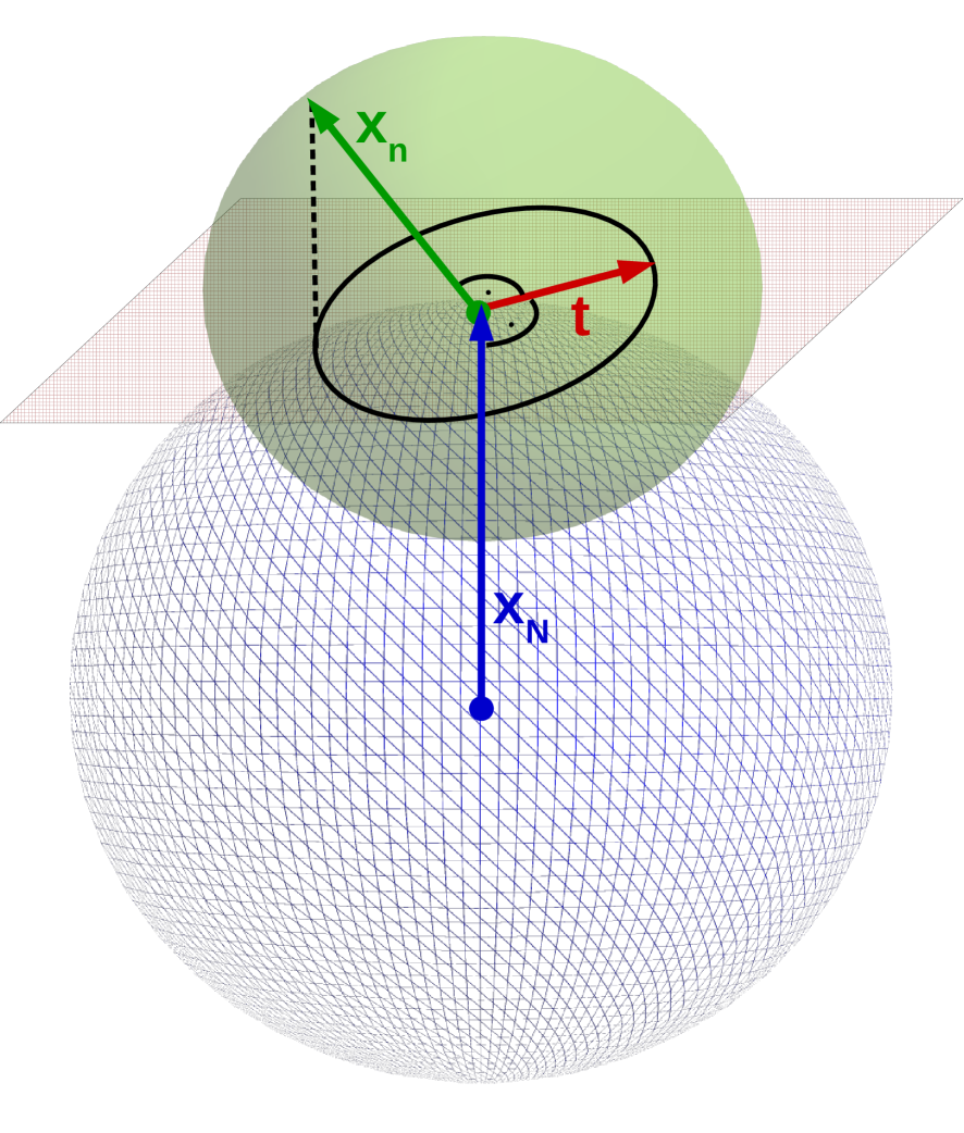
(a)

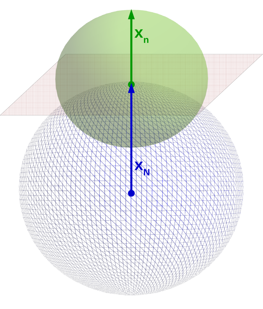
(b)

Figure 1: Sketched geometry of the coordinates $(x_{N},x_{n},t)$ for fixed ${\cal R}^{2}$. (a) For $x_{N}\nparallel x_{n}$, $x_{N}$ sweeps out a large (blue shaded) sphere $S^{4}_{N}$ and $x_{n}$ sweeps out a smaller (green) sphere $S_{n}^{4}$. $t$ lies in the (red) tangent space of $S^{4}_{N}$ at a point $x_{N}$. The projection of $x_{n}$ onto the tangent space yields the sphere $S^{2}_{\cal R}$. (b) For $x_{N}\parallel x_{n}$, the projection of $x_{n}$ onto the tangent space vanishes, i.e. $t$ is not a meaningful coordinate.

Since both $\tilde{\cal O}_{\Lambda}$ and ${\cal O}_{\Lambda}$ are 10-dimensional, this provides also a faithful local description of ${\cal O}_{\Lambda}$ for generic points. However, the map (3.44) is not injective, and it turns out to be a degenerate triple cover at least near $t=0$. This will be elaborated next.

$SU(3)$ structure and degeneracy.

To resolve the extremal values of ${\cal R}^{2}$ and to exhibit the global structure, consider the reference point $\xi=H_{\Lambda}\in\tilde{\cal O}_{\Lambda}$. This corresponds to $x_{N}=Ne_{5},x_{n}=ne_{5}$ and $t=0$ as 5-vectors, which is a non-generic case in the above description since ${\cal R}^{2}$ takes its maximum value. We will exhibit the triple covering structure over $(x_{N},x_{n},t)$ near $t=0$.

Following the general analysis, the projection $P_{N}$ maps $\xi$ to $\xi_{N}=H_{N\Lambda_{1}}$, which is a point in ${\mathbb{C}}P^{3}={\cal O}_{N\Lambda_{1}}=SU(4)/SU(3)\times U(1)$ described by $m_{N}^{ab}$. Denote with ${\cal K}$ its $SU(3)$ stabilizer, which is explicitly given by the $6\times 6$ matrices in (2.15). Note that this $SU(3)$ does not respect ${\cal R}^{2}$, and it provides the missing local parametrization (replacing $t$) of ${\cal O}_{\Lambda}$ near $\xi$. ${\cal K}$ acts on the symmetric $\tilde{t}^{ab}$ on ${\cal O}_{\Lambda}$ via

$$\tilde{t}^{ab}=\frac{1}{2}Nn\,(U\mathrm{diag}(\mbox{1 \kern-5.89996pt{\rm l}}_{2},-\mbox{1 \kern-5.89996pt{\rm l}}_{2},\mbox{1 \kern-5.89996pt{\rm l}}_{2})U^{-1})^{ab}\ ,\qquad U\in SU(3)\subset SO(6)$$ (3.48)

and similarly on $t^{a}$. We focus on the linearized action of $U=e^{i\lambda}$ on $\tilde{t}^{ab}_{0}=\mathrm{diag}(\mbox{1 \kern-5.89996pt{\rm l}}_{2},-\mbox{1 \kern-5.89996pt{\rm l}}_{2},\mbox{1 \kern-5.89996pt{\rm l}}_{2})$. Since the diagonal (Cartan) generators act trivially on $\tilde{t}^{ab}_{0}$, it suffices to consider the six root generators of $\mathfrak{su}(3)$, which we denote by

$$T_{1}^{+}=\begin{pmatrix}0&\mbox{1 \kern-5.89996pt{\rm l}}_{2}&0\\ 0&0&0\\ 0&0&0\end{pmatrix},\qquad T_{2}^{+}=\begin{pmatrix}0&0&0\\ 0&0&\mbox{1 \kern-5.89996pt{\rm l}}_{2}\\ 0&0&0\end{pmatrix},\qquad T_{3}^{+}=\begin{pmatrix}0&0&\mbox{1 \kern-5.89996pt{\rm l}}_{2}\\ 0&0&0\\ 0&0&0\end{pmatrix}=[T_{1}^{+},T_{2}^{+}]$$ (3.49)

and similarly $T_{i}^{-}=(T_{i}^{+})^{\dagger}$. We note that

$$=-2T_{1}^{+},\qquad[T_{2}^{+},\mathrm{diag}(\mbox{1 \kern-5.89996pt{\rm l}}_{2},-\mbox{1 \kern-5.89996pt{\rm l}}_{2},\mbox{1 \kern-5.89996pt{\rm l}}_{2})]=2T_{2}^{+},$$ (3.50)

$$[T_{3}^{\pm},\mathrm{diag}(\mbox{1 \kern-5.89996pt{\rm l}}_{2},-\mbox{1 \kern-5.89996pt{\rm l}}_{2},\mbox{1 \kern-5.89996pt{\rm l}}_{2})] =0\ .$$

This means that $SU(3)$ rotations generated by $\lambda=z_{1}T_{1}^{+}+z_{1}^{*}T_{1}^{-}+z_{2}T_{2}^{+}+z_{2}^{*}T_{2}^{-}$ will generate a 4-dimensional orbit through $\tilde{t}^{ab}_{0}$ parametrized by $(z_{1},z_{2})\in{\mathbb{C}}^{2}$. This provides the missing 4 local coordinates on ${\cal O}_{\Lambda}\sim{\mathbb{C}}P^{3}\times{\mathbb{C}}P^{2}$, complementing the local $S^{4}\times S^{2}$ description of ${\mathbb{C}}P^{3}$. However, this local patch of ${\mathbb{C}}P^{2}$ is mapped by $(t^{a})$ degenerately to ${\mathbb{R}}^{2}_{34}\subset{\mathbb{R}}^{4}$ via $t^{1}=t^{2}=0$, $t^{4}+it^{3}=z_{2}$, since the $T_{1}^{\pm}$ direction are not seen by $t^{a}$. These missing $T_{1}^{\pm}$ directions could be resolved by including, for example,

$$s^{3}=\tilde{t}^{13},\quad s^{4}=\tilde{t}^{14}$$ (3.51)

as extra embedding coordinates. Then $(t^{1},t^{2},t^{3},t^{4},s^{3},s^{4})$ describes precisely the squashed ${\mathbb{C}}P^{2}$ as discussed in [22, 21], which has a triple self-intersection at the origin as in Figure 2(a).

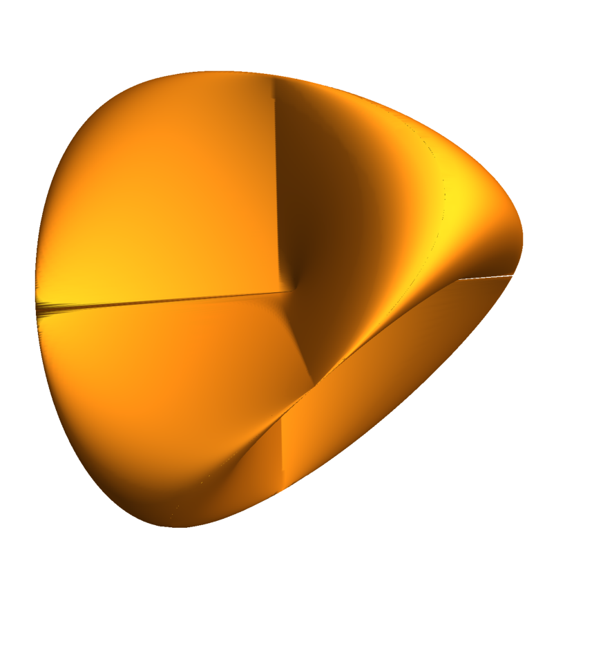
(a)

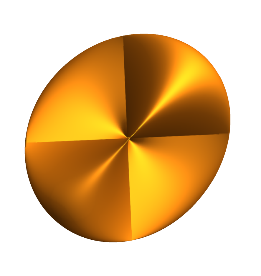
(b)

Figure 2: (a) Squashed ${\mathbb{C}}P^{2}$ described by $(t^{1},t^{2},t^{3},t^{4},s^{3},s^{4})$, with triple self-intersection. (b) Squashed ${\mathbb{C}}P^{2}$ described by $(t^{1},t^{2},t^{3},t^{4})$, with degenerate covering.

Projecting out the $s^{3,4}$ leads to a further projection along 2 of the 6 directions.

To see the global structure, consider the Weyl group ${\cal W}$ of $SU(3)$, which acts by permuting these $2\times 2$ matrix blocks in (3.48). ${\cal W}$ is generated by three reflections $w_{1,2,3}$, which map $\xi$ to 2 other points $w_{1}\xi,w_{3}\xi$ as follows

$$w_{1}\tilde{t}^{ab}_{0}=\mathrm{diag}(-\mbox{1 \kern-5.89996pt{\rm l}}_{2},\mbox{1 \kern-5.89996pt{\rm l}}_{2},\mbox{1 \kern-5.89996pt{\rm l}}_{2}),\qquad w_{2}\tilde{t}^{ab}_{0}=\tilde{t}^{ab}_{0},\qquad w_{3}\tilde{t}^{ab}_{0}=\mathrm{diag}(\mbox{1 \kern-5.89996pt{\rm l}}_{2},\mbox{1 \kern-5.89996pt{\rm l}}_{2},-\mbox{1 \kern-5.89996pt{\rm l}}_{2})\ .$$ (3.52)

By inspection, ${\cal W}$ preserves $x_{N}$ and $x_{n}$ at the reference point $\xi$, which means that these 3 distinct points on ${\cal O}_{\Lambda}$ have the same coordinates $(x_{N},x_{n},t)$. This shows the 3-fold covering structure near $t=0$. We have already seen that the local patch of ${\mathbb{C}}P^{2}$ near $\xi$ is mapped by $t$ to ${\mathbb{R}}^{2}_{34}\subset{\mathbb{R}}^{4}$, providing a degenerate partial cover of the $t$ coordinates near 0. Similarly, the local patch near $w_{1}\xi$ described by $SU(3)$ rotations generated by $\lambda=z_{1}T_{1}^{+}+z_{1}^{*}T_{1}^{-}+z_{3}T_{3}^{+}+z_{3}^{*}T_{3}^{-}$ is given by

$$=2T_{1}^{+},\qquad[T_{3}^{+},\mathrm{diag}(-\mbox{1 \kern-5.89996pt{\rm l}}_{2},\mbox{1 \kern-5.89996pt{\rm l}}_{2},\mbox{1 \kern-5.89996pt{\rm l}}_{2})]=2T_{3}^{+},$$ (3.53)

$$[T_{2}^{\pm},\mathrm{diag}(-\mbox{1 \kern-5.89996pt{\rm l}}_{2},\mbox{1 \kern-5.89996pt{\rm l}}_{2},\mbox{1 \kern-5.89996pt{\rm l}}_{2})] =0\ ,$$

which is mapped by $(t^{a})$ degenerately to ${\mathbb{R}}^{2}_{12}\subset{\mathbb{R}}^{4}$ via $t^{1}+it^{2}=z_{3}$, $t^{4}=t^{3}=0$. In contrast, the local patch near $w_{3}\xi$ described by $SU(3)$ rotations generated by $\lambda=z_{2}T_{2}^{+}+z_{2}^{*}T_{2}^{-}+z_{3}T_{3}^{+}+z_{3}^{*}T_{3}^{-}$ is given by

$$=-2T_{2}^{+},\qquad[T_{3}^{+},\mathrm{diag}(\mbox{1 \kern-5.89996pt{\rm l}}_{2},\mbox{1 \kern-5.89996pt{\rm l}}_{2},-\mbox{1 \kern-5.89996pt{\rm l}}_{2})]=-2T_{3}^{+},$$ (3.54)

$$[T_{1}^{\pm},\mathrm{diag}(\mbox{1 \kern-5.89996pt{\rm l}}_{2},\mbox{1 \kern-5.89996pt{\rm l}}_{2},-\mbox{1 \kern-5.89996pt{\rm l}}_{2})] =0\ ,$$

which is non-degenerately mapped to ${\mathbb{R}}^{4}$ by $t^{1}+it^{2}=z_{3}$, $t^{4}+it^{3}=z_{2}$.

To summarize, the map $t:{\cal O}_{\Lambda}\to{\mathbb{R}}^{4}$ near $t=0$ is a triple covering as illustrated in Figure 2(b), which is a projection of squashed ${\mathbb{C}}P^{2}$ to ${\mathbb{R}}^{4}$.

This self-intersecting structure is very interesting. It suggests that the low-energy physics on $S^{4}$ will have 3 generations, which arise from fermionic strings connecting these 3 sheets at the origin $t=0$. This is very close to the situation studied in [22, 21], where a similar squashed fuzzy ${\mathbb{C}}P^{2}$ led to 3 generations with low-energy physics not far from the Standard Model. Interestingly, here we would expect 2+1 generations, since the string connecting the two degenerate sheets is different from the 2 strings connecting one degenerate sheet with the regular sheet. As in [22, 21], these fermionic modes are expected to be chiral. It is tempting to relate this to the fact that there are 2 light and 1 heavy generations in the Standard Model. This is one of the intriguing aspects of the present background, further improving the picture of [22, 21].

3.3 Poisson brackets

We define

$$\tilde{x}^{a}=\tilde{m}^{a6}=({\bf m}^{3})^{a6}\ .$$ (3.55)

From the basic Poisson brackets (2.8), we obtain

$$\{x^{a},\tilde{x}^{c}\} =\tilde{m}^{ac}\;,$$ (3.56)

$$\{t^{a},x^{c}\} =t^{ac}-{\cal R}^{2}g^{ac}=\tilde{t}^{ac}-2\delta\,g^{ac}\;,$$

$$\{t^{a},t^{c}\} =-{\cal R}^{2}\,m^{ac}-\tilde{m}^{ac}-x^{a}t^{c}+t^{a}x^{c}\;,$$

$$\{t^{a},\tilde{x}^{c}\} =\frac{1}{2}(N^{2}+n^{2})\big{(}{\cal R}^{2}\,g^{ac}-t^{ac}\big{)}+\tilde{x}^{a}x^{c}-x^{a}\tilde{x}^{c}\;,$$

for $a,c\neq 6$. Here, $\delta=x_{N}\cdot x_{n}$ as defined in (3.27), and we used

$$\tilde{x}\cdot x =-\frac{1}{2}(N^{2}+n^{2}){\cal R}^{2}+\frac{1}{16}(N^{2}-n^{2})^{2}\ .$$ (3.57)

which follows from (3.36).

To compare with the fuzzy case, we also compute the following double Poisson brackets:

$$\sum_{a=1}^{5}\{x^{a},\{x^{a},x^{c}\}\}= -4x^{c}\;,$$ (3.58a)

$$\sum_{a=1}^{5}\{t^{a},\{t^{a},t^{c}\}\}= -\left(3(N^{2}+n^{2})+\mbox{Tr}(t)\right)t^{c}+12{\cal R}^{2}t^{c}$$

$$= -\frac{1}{2}\left(9N^{2}+2Nn+9n^{2}\right)t^{c}+12{\cal R}^{2}t^{c}\;.$$ (3.58b)

As emphasized before, the Poisson structure lives on the bundle space ${\cal O}_{\Lambda}$, and does not respect the various projections to $S^{4}$. However, it can be viewed as a bundle of Poisson structures on $S^{4}$, giving rise to a frame bundle on $S^{4}$ as emphasized in [1].

Radial constraint and $y$ variables.

We can now identify generators which commute with ${\cal R}^{2}$. This would allow to impose the radial constraint

$${\cal R}^{2}=\mathrm{const}\,,$$ (3.59)

which defines a generalized irreducible $SO(5)$ sphere. From the above Poisson brackets, we obtain

$$\{{\cal R}^{2},x^{a}\} =2x_{b}m^{ba}=2t^{a}\;,$$ (3.60)

$$\{{\cal R}^{2},\tilde{x}^{a}\} =2x_{b}\tilde{m}^{ba}=-(N^{2}+n^{2})t^{a}\;,$$

$$\{{\cal R}^{2},t^{a}\} =2x_{b}(t^{ba}-{\cal R}^{2}g^{ba})=-2\tilde{x}^{a}-2{\cal R}^{2}x^{a}\;,\qquad a\neq 6$$

and we see that the following generators $y^{a}$ commute with ${\cal R}^{2}$:

$$\{{\cal R}^{2},y^{a}\} =0\ ,$$ (3.61)

$$y^{a} \coloneqq\frac{2}{N^{2}-n^{2}}\big{(}(N^{2}+n^{2})x^{a}+2\tilde{x}^{a}\big{)}=x_{N}^{a}-x_{n}^{a}\ .$$

This means that wave functions $\phi(y^{a})$ strictly respect ${\cal R}^{2}$. In particular, a semi-classical Laplacian chosen as

$$\Box_{y}\coloneqq-\{y^{a},\{y_{a},\cdot\}\}$$ (3.62)

(compare to fuzzy case (5.2)) induces no kinetic term in the radial dimensions, and $\Box_{y}y^{a}$ Poisson-commutes with ${\cal R}^{2}$. Therefore,

$$\Box_{y}y^{a}=c_{1}y^{a}+c_{2}{\cal R}^{2}y^{a}\$$ (3.63)

for suitable constants $c_{1},c_{2}$. This corresponds to (5.20) in the fuzzy case. Furthermore, the above Poisson brackets imply

$$\{t^{a},y^{b}\} =y^{a}x^{b}-x^{a}y^{b}\;,$$ (3.64a)

$$\{y^{a},y^{b}\} =\frac{4}{N^{2}-n^{2}}\,\left(\left(\frac{N^{2}+n^{2}}{2}-{\cal R}^{2}\right)y^{ab}+y^{a}t^{b}-t^{a}y^{b}\right)\;,$$ (3.64b)

where

$$y^{ab}\coloneqq m_{N}^{ab}-m_{n}^{ab}$$ (3.64c)

in analogy to (3.61). In particular, this means that

$$\{t^{\mu},y^{\nu}\}=0,\qquad\mu,\nu=1,\ldots,4$$ (3.65)

in tangential coordinates where e.g. $x^{a}\sim e_{5}$. Thus, $t$ can be viewed as momentum generator for either of $x_{N}$, $x_{n}$ or $x$, but not for $y$.

We also note the following constraints:

$$\{y^{a},y^{b}\}y_{b} =0\ ,$$ (3.66)

$$m^{ab}y_{b} =m^{ab}(x_{b}+\frac{2}{N^{2}+n^{2}}\tilde{x}^{a}_{b})=0$$

from (3.36). This means that imposing ${\cal R}^{2}=\mathrm{const}$ is incompatible with the gravity mechanism discussed in [1], as for the basic fuzzy 4-sphere. We will, therefore, not impose this constraint. In contrast, $t^{a}$ does not commute with ${\cal R}^{2}$.

There is an interesting alternative approach to the $y^{a}$ generators: Consider

$$e^{ab}=\epsilon^{abcdef}m^{cd}m^{ef},\qquad e^{a}=e^{a6}\;.$$ (3.67)

By anti-symmetry, $e^{ab}$ must be a linear combination of $m^{ab}$ and $\tilde{m}^{ab}$; hence, $e^{a}$ must be a linear combination of $x_{N}^{a}$ and $x_{n}^{a}$. Since it Poisson-commutes with ${\cal R}^{2}$, it follows that

$$y^{a}\sim e^{a}\ .$$ (3.68)

3.4 Summary of Poisson brackets

To facilitate the comparison with the fuzzy case, we collect the basic relations for the Poisson brackets on the classical orbit ${\cal O}_{\Lambda}$ here:

$$\{x^{a},x^{b}\} =m^{ab}\;,$$ (3.69)

$$\{x^{a},y^{b}\} =y^{ab}\coloneqq m_{N}^{ab}-m_{n}^{ab}\;,$$

$$\{x^{a},t^{b}\} =-\tilde{t}^{ab}+2\delta\,g^{ab}\;,$$

$$\{y^{a},y^{b}\} =\frac{4}{N^{2}-n^{2}}\,\left(\left(\frac{N^{2}+n^{2}}{2}-{\cal R}^{2}\right)y^{ab}+y^{a}t^{b}-t^{a}y^{b}\right)\;,$$

$$\{t^{a},t^{b}\} =\Big{(}\frac{N^{2}+n^{2}}{2}-{\cal R}^{2}\Big{)}\,m^{ab}-\frac{N^{2}-n^{2}}{4}\,y^{ab}-x^{a}t^{b}+t^{a}x^{b}\;,$$

$$\{t^{a},y^{b}\} =y^{a}x^{b}-x^{a}y^{b}\;,$$

where $a,b=1,\ldots,5$.

3.5 Functions on ${\cal S}^{4}_{\Lambda}$

Local coordinates.

We restrict ourselves to generic points where $x_{N}$ and $x_{n}$ are linearly independent. As discussed in Section 3.2, this means that $x_{N}$, $x_{n}$, and $t$ provide a good local description of ${\cal O}_{\Lambda}$. Hence, all functions can be represented locally as $\phi(x_{N},x_{n},t)$. In particular, the $5\times 5$ matrices $m_{N}^{ab},\tilde{m}_{n}^{ab}$ and $t^{ab}$ can be expressed in terms of $x_{N},x_{n},t$ as follows: Their action on $x_{N},x_{n},t$ is obtained from (3.38), which implies that $m_{N}$ and $m_{n}$ respect this $3\times 3$ block-structure. The remaining antisymmetric $2\times 2$ block can then be written in terms of

$$f^{ab} :=\epsilon^{abcde}x_{N}^{c}x_{n}^{d}t^{e}\ =-f^{ba}\ ,\quad\qquad 0=f_{ab}x_{N}^{a}=f_{ab}x_{n}^{a}=f_{ab}t^{a}\ .$$ (3.70)

Explicitly, one finds

$$m_{N}^{ab} =\frac{2}{t\cdot t}(v_{N}^{a}t^{b}-t^{a}v_{N}^{b})+d_{N}f^{ab}\,,$$ (3.71a)

$$m_{n}^{ab} =\frac{2}{t\cdot t}(v_{n}^{a}t^{b}-t^{a}v_{n}^{b})+d_{n}f^{ab}\,,$$ (3.71b)

where

$$v_{N} =\frac{N^{2}}{4}x_{n}-\delta\ x_{N}\,,\qquad v_{N}\cdot x_{N}=0\,,\quad v_{N}\cdot v_{N}=\frac{N^{2}}{16}t\cdot t\,,$$ (3.71c)

$$v_{n} =\frac{n^{2}}{4}x_{N}-\delta\ x_{n}\,,\ \qquad v_{n}\cdot x_{n}\ =0\,,\ \quad v_{n}\cdot v_{n}\ =\frac{n^{2}}{16}t\cdot t\,,$$ (3.71d)

and $d_{N,n}$ can be computed from the (anti)self-duality of $m_{N,n}$ at $x_{N,n}$. The matrix $t^{ab}$ could be determined similarly. However, this description does not work if $x$ and $y$ are parallel. We can then use, for instance, $m^{ab}$ to complement $x$ and $t$, which may be useful also more generally.

Explicit local coordinates on ${\cal O}_{\Lambda}$ can be found as follows: Since ${\cal O}_{\Lambda}$ is a homogeneous space, we can pick any given reference point $p\in{\cal O}_{\Lambda}$. Such a reference point could be

$$x_{N}=e_{5}R_{N},\quad x_{n}=R_{n}(\cos\vartheta e_{5}+\sin\vartheta e_{4}),\quad\ t=R_{t}e_{3}$$ (3.72)

where $R_{t}$ can be extracted from (3.45). We can then use $x_{N}^{1,\ldots,4}$, $x_{n}^{1,2,3}$, and $t^{1,2}$ as local coordinates. The missing $10^{\mathrm{th}}$ coordinate is provided by $\vartheta$.

Finally, we note that the only $SO(5)$-invariant functions on ${\cal O}_{\Lambda}$ are given by $f({\cal R}^{2})$.

Bundle structure and higher spin.

We want to describe the fluctuation modes on ${\cal O}_{\Lambda}$ in a $SO(5)$-covariant way, reflecting the local bundle structure $S^{4}\times{\cal K}$. We will consider $S^{4}\ni x$ as physical configuration space, and use $\xi$ to describe points on ${\cal K}$ in the following.

In standard Kaluza-Klein (KK) compactification, the harmonics on ${\cal K}$ yield a KK tower of scalar fields on $S^{4}$. However, in the present situation $SO(5)$ acts on both $S^{4}$ and ${\cal K}$, which form a twisted (equivariant) bundle. This means that functions $\phi(x,\xi)\in{\cal C}(S^{4}\times{\cal K})\cong{\cal C}(S^{4})\otimes{\cal C}({\cal K})$ must be decomposed as tensor product of $SO(5)$ reps, which leads to a tower of higher spin modes on $S^{4}$ instead of the usual KK tower. This twisted structure is the crucial point of these covariant backgrounds. It transmutes KK modes into, for example, gravitons and other higher spin modes with the appropriate local transformation properties.

Mode expansion.

With this in mind, we want to represent functions on ${\cal O}_{\Lambda}$ as functions on $S^{4}$ expanded into the harmonics on ${\cal K}$. An $SO(5)$-covariant way to organize functions on $S^{4}\times{\cal K}$ is as follows:

$$\phi =\phi(x,t,y)$$

$$=\phi(x,t)+\phi_{ab}(x,t)m^{ab}+\phi_{ab;cd}(x,t)m^{ab}m^{cd}+\ldots\;,$$ (3.73)

see for instance [1]. These modes can be expanded further in polynomials in $t$ as

$$\phi_{ab}(x,t)=\varphi_{ab}(x)+\varphi_{ab;e}(x)t^{e}+\varphi_{ab;ef}(x)t^{e}t^{f}+\ldots$$ (3.74)

etc. The $\varphi_{ab;e}(x)$ etc. clearly describe some higher spin theory on $S^{4}$, and it would be desirable to make contact with (Vasiliev-type [30]) higher spin theories. To understand the role of possible radial contributions, consider e.g. $\phi_{ab}(x)=h_{a}(x)x_{b}-h_{b}(x)x_{a}$. Then

$$\phi_{ab}m^{ab} =(h_{a}(x)x_{b}-h_{b}(x)x_{a})m^{ab}=-2h_{a}t^{a}$$ (3.75)

recalling $t=-{\bf m}\cdot x$. Hence, radial components of $\phi_{ab}$ give rise to $t^{a}$, which is included in (3.74). To avoid over-counting, $\phi_{ab;cd}$ should, therefore, be tangential on $S^{4}$ and traceless.

Dimensional reduction.

The above $SO(5)$ organization is not sufficient to guarantee a truly 4-dimensional theory. The dynamics is governed by $\Box$ (5.2), which is some Laplace operator on the 10-dimensional space ${\cal O}_{\Lambda}$. An effectively 4-dimensional theory is obtained via dimensional reduction on ${\cal K}$: if only the trivial mode on ${\cal K}$ participates (or dominates), then the wavefunctions are given by $\phi(x)$, depending only on $x$, and $\Box$ reduces to a Laplace operator on the large $S^{4}$. More precisely, initial configurations which are (almost) constant on ${\cal K}$ should remain so under the dynamics.

There are different possibilities to justify this scenario. One possibility is a large mass gap on ${\cal K}$, so that excitations along ${\cal K}$ do not play an important role at low energies. This requires a large asymmetry in $\Box$. While this is natural for $n\ll N$, it depends on the embedding of the background in the matrix model, which can be reliably addressed only once the effective potential including quantum corrections is sufficiently well understood.

We will encounter also another – in a sense dual – mechanism for dimensional reduction: Assume that only 5 matrices are embedded, as in the background ${\cal Y}^{A}\sim(T^{a},0)^{T}$ considered in Section 5.2. Then the effective metric on ${\cal O}_{\Lambda}$ has reduced rank (rather than full rank 10) and is restricted to $x$ space, while no kinetic term in the $y$ direction is induced. The internal modes in $y$ space are clearly higher spin modes whose propagation is only 4-dimensional. More generally, embeddings such as ${\cal Y}^{A}\sim(T^{a},Y^{a})^{T}$ where one scale is much larger than the other would naturally lead to dimensional reduction.

Dimensional reduction is further supported by the fact that excitations on ${\cal K}$ couple only via derivatives to functions on $S^{4}$, which is suppressed at low energies by the scale of non-commutativity. These non-trivial ${\cal K}$ modes include the spin 2 gravitons on $S^{4}$, and the higher spin modes will be suppressed even more. However this is a complicated issue which can be settled only if the background geometry is known.

Averaging.

To compute the low-energy observables in this dimensional reduction scheme, one needs to project on functions which are constant in ${\cal K}$. This can be done by ”averaging“ over ${\cal K}$ as follows: Consider any given point (the ”north pole“) $p\in S^{4}$. As discussed before, the fiber ${\cal K}$ over $p$ is the orbit of its stabilizer $SO(4)\subset SO(5)$. Thus, averaging over this fiber is tantamount to averaging over the local $SO(4)$ stabilizer, and is denoted by

$$[f(x,\xi)]_{0}\ .$$ (3.76)

By construction, the result is a scalar of the local stabilizer $SO(4)$. Carrying this out over each point, one obtains e.g.

$$[t^{ab}]_{0}=\frac{1}{4}N^{2}\left(g^{ab}+{\cal O}\left(\frac{1}{N}\right)\right)\ ,\qquad[m^{ab}]_{0}=0=[y^{ab}]_{0}\ ,\qquad a,b=1,\ldots,5\;.$$ (3.77)

4 Fuzzy geometry

The results of the previous sections provide the guideline for organizing the corresponding fuzzy algebra, and for finding embeddings which are solutions of IKKT-type matrix models.

4.1 Fuzzy operator algebra

The algebra $\mathrm{End}({\cal H})$ of functions on fuzzy ${\cal S}^{4}_{\Lambda}$ is properly understood as quantized algebra of functions on ${\cal O}_{\Lambda}$, which decomposes into the direct sum of higher spin harmonics on $S^{4}$. For the basic fuzzy sphere $S^{4}_{N}$ with $\Lambda=(N,0,0)$, the underlying orbit is ${\mathbb{C}}P^{3}$, and the fuzzy algebra of functions is

$$\mathrm{End}({\cal H}_{N})=(0,0,N)\otimes(N,0,0) =\bigoplus\limits_{n\leq N}(n,0,n)_{\mathfrak{so}(6)}$$

$$\cong\bigoplus\limits_{m\leq n\leq N}(n-m,2m)_{\mathfrak{so}(5)}\ ,$$ (4.1)

cf. [29]. This is the twisted analog of a KK tower with intrinsic UV cutoff; for example, ${\cal M}^{ab}\in(1,0,1)$. For the generalize fuzzy spheres with $\Lambda=(N,0,n)$, additional modes arise, and some multiplicities become non-trivial. It turns out that the following structure holds for the lowest modes:

$$\mathrm{End}({\cal H}_{\Lambda}) =(n,0,N)\otimes(N,0,n)=(0,0,0)\oplus 2(1,0,1)\oplus(0,2,0)\oplus\ldots$$ (4.2)

provided $N,n>0$.

Automorphism.

There is an involutive anti-linear automorphism given by

$$\sigma({\cal M}^{ab})=-{\cal M}^{ab}\,,\qquad\sigma(i)=-i\,,$$ (4.3a)

which satisfies

$$\sigma(\tilde{\cal M}^{ab})=-\tilde{\cal M}^{ab}\,,\qquad\sigma({\cal T}^{ab})={\cal T}^{ab}\,.$$ (4.3b)

On $\mathrm{End}({\cal H})$, this automorphism is nothing but complex conjugation, but it helps to understand better the algebraic properties in the fuzzy case, such as $\Box T\sim T$ etc.

Matrix operators.

We will now identify the fuzzy analogs ${\cal M}^{ab}$, $\tilde{\cal M}^{ab}$, and ${\cal T}^{ab}$ of the anti-symmetric resp. symmetric matrix-valued functions $m^{ab}$, $\tilde{m}^{ab}$, and $T^{ab}$. The operators are defined by the same (anti)symmetry and trace conditions as their classical counterparts. First, ${\cal T}^{ab}$ is defined to be the symmetric traceless part of ${\cal M}^{2}$,

$${\cal T}^{ab}\coloneqq-({\cal M}^{2})^{\{ab\}} =\frac{1}{2}\{{\cal M}^{ac},{\cal M}^{bc^{\prime}}\}_{+}\ g_{cc^{\prime}}=-({\cal M}^{2})^{ab}-2i{\cal M}^{ab}\,,$$ (4.4)

using the Lie algebra relations in the last line. It then follows that

$$({\cal T}^{ab})^{*}={\cal T}^{ab}={\cal T}^{ba}$$ (4.5a)

and

$${\cal T}^{66}={\cal R}^{2}\,.$$ (4.5b)

${\cal T}^{ab}$ is, in fact, the unique $(0,2,0)$ tensor operator in $\mathrm{End}({\cal H}_{\Lambda})$ for $\Lambda=(N,0,n)$, and it vanishes for $\Lambda=(N,0,0)$.

Similarly, $\tilde{\cal M}^{ab}$ is defined to be the anti-symmetric part of ${\cal M}^{3}$,

$$\tilde{\cal M}^{ab}\coloneqq({\cal M}^{3})^{[ab]} =\frac{1}{2}({\cal M}^{ac}{\cal M}^{cd}{\cal M}^{db}-{\cal M}^{bc}{\cal M}^{cd}{\cal M}^{da})$$ (4.6)

$$=({\cal M}{\cal M}{\cal M})^{ab}+5i({\cal M}{\cal M})^{ab}-10{\cal M}^{ab}-\frac{i}{2}(\mbox{Tr}{\cal M}^{2})\,g^{ab}\,,$$

using again the Lie algebra relations in the last line. Again, it follows that

$$(\tilde{\cal M}^{ab})^{*}=\tilde{\cal M}^{ab}=-\tilde{\cal M}^{ba}.$$ (4.7)

The story of independent monomials of ${\cal M}$ ends here, since ${\cal M}^{4}$ can be expressed in terms of the above matrix generators via its characteristic equation. This arises as follows:

Characteristic equation.

Since $\mathrm{End}({\cal H}_{\Lambda})$ is a quantization of the algebra of functions on ${\cal O}_{\Lambda}$, its decomposition into harmonics is the same below the cutoff $N$. For the generalized spheres, we note that the decomposition (4.2) contains only two $(1,0,1)$ operators. These must be given by ${\cal M}^{ab}$ and $\tilde{\cal M}^{ab}$. Furthermore, there is only one $(0,2,0)$ operators, which must be ${\cal T}^{ab}$. Therefore, ${\cal M}$, ${\cal T}$, $\tilde{\cal M}$, and $g$ form a closed matrix algebra. In other words, ${\cal M}$ satisfies a characteristic equation of order 4, which is the matrix analog of (3.35). For $\Lambda=(N,0,n)$, it takes the form (see Appendix A.1 for a derivation)

$$\left(\left(i{\cal M}+2\right)^{2}-\frac{(N-n)^{2}}{4}\right)\left(\left(i{\cal M}+\frac{3}{2}\right)^{2}-\frac{(N+n+3)^{2}}{4}\right)=0\ .$$ (4.8)

This is clearly consistent with (3.35) up to quantum corrections. Accordingly, there are two independent Casimirs, given by

$$C_{2}[\mathfrak{so}(6)]=-\frac{1}{2}\mbox{Tr}({\cal M}^{2})=\frac{1}{2}\mbox{Tr}({\cal T}),\qquad C_{3}[\mathfrak{so}(6)]=\mbox{Tr}({\cal M}^{3}),$$ (4.9)

while the higher Casimirs reduce to the above via the characteristic equation. Moreover, the characteristic equation implies

$$\tilde{\cal M}{\cal M}={\cal M}\tilde{\cal M}=-2i\tilde{\cal M}+R_{\tilde{\cal M}{\cal M}}^{T}{\cal T}+R_{\tilde{\cal M}{\cal M}}^{g}\,g\ .$$ (4.10)

The coefficients of the anti-symmetric terms ${\cal M}$, $\tilde{\cal M}$ on the rhs follow directly from

$${\cal M}_{ac}\tilde{\cal M}_{cb}-\tilde{\cal M}_{bc}{\cal M}_{ca} =[{\cal M}_{ac},\tilde{\cal M}_{cb}]=-4i\tilde{\cal M}^{ab}\,,$$ (4.11)

which implies that there is no ${\cal M}$ term in (4.10). The remaining coefficients $R_{\tilde{\cal M}{\cal M}}^{T},R_{\tilde{\cal M}{\cal M}}^{g}$ are found to be

$$R_{\tilde{\cal M}{\cal M}}^{T} =-\frac{1}{2}\left(N^{2}+n^{2}+3N+3n+8\right),$$ (4.12a)

$$R_{\tilde{\cal M}{\cal M}}^{g} =-\frac{1}{16}(N-n)^{2}(N+n+4)(N+n+2)$$

$$=\ \frac{1}{6}\,\left(\mbox{Tr}\left({\cal M}^{4}\right)+\left(R_{\tilde{\cal M}{\cal M}}^{T}-10\right)\,\mbox{Tr}({\cal M}^{2})\right)\;.$$ (4.12b)

Now, one can work out the full matrix multiplication algebra of the $\tilde{\cal M}$, ${\cal T}$, ${\cal M}$, and $g$. This will be given for the modified basis ${\cal M}_{N}$, ${\cal M}_{n}$ as determined below.

Vector operators.

As in the commutative case, we can define the $SO(5)$ vector operators

$$X^{a} ={\cal M}^{a6},\qquad\tilde{X}^{a}=\tilde{\cal M}^{a6},\qquad T^{a}=\tilde{\cal T}^{a6}\$$ (4.13)

for $a=1,\ldots,5$, which provide possible embeddings of generalized fuzzy spheres in the matrix model. We can compute their scalar products by taking the $66$ component of the above matrix multiplication algebra. For example, (4.10) implies

$$\tilde{X}\cdot X=-R_{\tilde{\cal M}{\cal M}}^{T}\,{\cal R}^{2}-R_{\tilde{\cal M}{\cal M}}^{g}=X\cdot\tilde{X}\,.$$ (4.14)

Similarly, one finds

$$X\cdot T+T\cdot X =0=\tilde{X}\cdot T+T\cdot\tilde{X}\,,$$ (4.15)

which is consistent with the semi-classical limit $x\cdot t=0$, see (3.39). The last relations state that $T^{a}$ is orthogonal to both $X^{a}$ and $\tilde{X}^{a}$. This follows immediately from

$$X\cdot T =-{\cal M}^{6a}{\cal T}^{a6}=-({\cal M}{\cal T})^{66}=-({\cal T}{\cal M})^{66}=-T\cdot X,$$ (4.16)

and similarly for $\tilde{X}$.

Matrix multiplication algebra.

As in the classical case (3.21), we would like to find operator-valued $6\times 6$ matrices

$${\cal M}_{N}^{ab},\qquad{\cal M}_{n}^{ab},\qquad\tilde{\cal T}^{ab}\coloneqq{\cal T}^{ab}-cg^{ab}\,,$$ (4.17)

where

$$\begin{pmatrix}{\cal M}_{N}\\ {\cal M}_{n}\end{pmatrix} \coloneqq\begin{pmatrix}\alpha_{N}&\beta_{N}\\ \alpha_{n}&\beta_{n}\end{pmatrix}\begin{pmatrix}\tilde{{\cal M}}\\ {\cal M}\end{pmatrix}\equiv A\begin{pmatrix}\tilde{{\cal M}}\\ {\cal M}\end{pmatrix}\;.$$ (4.18)

The associated vector operators

$$X_{N}^{a} ={\cal M}_{N}^{a6}\,,\qquad\tilde{X}^{a}_{n}=\tilde{\cal M}^{a6}_{n}\,,\qquad\tilde{T}^{a}=\tilde{\cal T}^{a6}=T^{a}\,$$ (4.19)

for $a=1,\ldots,5$ are defined such that the inner products of the $X_{N,n}$ take the simple form

$$\begin{pmatrix}X_{N}\cdot X_{N}&X_{N}\cdot X_{n}\\ X_{N}\cdot X_{n}&X_{n}\cdot X_{n}\end{pmatrix}=\begin{pmatrix}R_{N}^{2}&0\\ 0&R_{n}^{2}\end{pmatrix}+\Delta\begin{pmatrix}0&1\\ 1&0\end{pmatrix},\qquad\Delta=\frac{1}{2}({\cal R}^{2}-c\mbox{1 \kern-5.89996pt{\rm l}})$$ (4.20)

for some suitable $c\in{\mathbb{R}}$. This is the fuzzy analog of (3.27), and it means that $X_{N}$ and $X_{n}$ describe two fuzzy 4-spheres with sharp radii $R^{2}_{N}$ and $R^{2}_{n}$, respectively.

The coefficients $\alpha_{N,n}$, $\beta_{N,n}$ are to be defined such that (4.20) holds. To carry this out, it is convenient to first rewrite the matrix algebra of ${\cal M}$, $\tilde{\cal M}$, and $\tilde{\cal T}$ in terms of the new operators ${\cal M}_{N}$, ${\cal M}_{n}$, and $\tilde{\cal T}$. Then the requirement (4.20) is tantamount to the vanishing of the three red coefficients in the following multiplication table:

$${\cal M}_{N}{\cal M}_{N} =iR_{NN}^{N}{\cal M}_{N}+iR_{NN}^{n}{\cal M}_{n}{\color[rgb]{1,0,0}{\;+0\cdot\tilde{\cal T}\;}}+R_{NN}^{g}g\;,$$ (4.21)

$${\cal M}_{n}{\cal M}_{n} =iR_{nn}^{N}{\cal M}_{N}+iR_{nn}^{n}{\cal M}_{n}{\color[rgb]{1,0,0}{\;+0\cdot\tilde{\cal T}\;}}+R_{nn}^{g}g\;,$$

$${\cal M}_{N}{\cal M}_{n}={\cal M}_{n}{\cal M}_{N} =iR_{Nn}^{N}{\cal M}_{N}+iR_{Nn}^{n}{\cal M}_{n}+R_{Nn}^{T}\tilde{\cal T}{\color[rgb]{1,0,0}{\;+0\cdot g\;}}\;,$$

$$\tilde{\cal T}{\cal M}_{N} ={\color[rgb]{0,0,1}{\;+0\cdot{\cal M}_{N}\;}}+R_{TN}^{n}{\cal M}_{n}+iR_{TN}^{T}\tilde{\cal T}+iR_{TN}^{g}\ g\;,$$

$$\tilde{\cal T}{\cal M}_{n} =R_{Tn}^{N}{\cal M}_{N}{\color[rgb]{0,0,1}{\;+0\cdot{\cal M}_{n}\;}}+iR_{Tn}^{T}\tilde{\cal T}+iR_{Tn}^{g}\ g\;,$$

$$\tilde{\cal T}\tilde{\cal T} =iR_{TT}^{N}{\cal M}_{N}+iR_{TT}^{n}{\cal M}_{n}+R_{TT}^{T}\tilde{\cal T}+R_{TT}^{g}\ g\;.$$

Requiring that $R_{NN}^{T}=0=R_{nn}^{T}$ yields the solutions

$$\beta_{N} =\frac{\alpha_{N}}{4}\left(2N^{2}+6N+2n^{2}+6n+16+\kappa(N-n)\sqrt{(N+n+4)(N+n+2)}\right)\;,$$ (4.22)

$$\beta_{n} =\frac{\alpha_{n}}{4}\left(2N^{2}+6N+2n^{2}+6n+16+\gamma(N-n)\sqrt{(N+n+4)(N+n+2)}\right)\;,$$

for $\kappa,\gamma=\pm 1$. For $A$ to be invertible, it follows from

$$\det{A} =\frac{1}{4}\alpha_{n}\alpha_{N}(\gamma-\kappa)(N-n)\sqrt{(N+n+4)(N+n+2)}\;$$ (4.23a)

that one has to choose $$\gamma\neq\kappa \gamma=-\kappa \kappa=\pm 1 N\leftrightarrow n$$. Thus, and the remaining freedom simply interchanges . The determinant reduces to

$$\det{A} =\alpha_{n}\alpha_{N}\kappa\det{\tilde{A}}$$ (4.23b)

$$\det{\tilde{A}} =\frac{n-N}{2}\sqrt{(N+n+4)(N+n+2)}\ =\ -2\sqrt{-R_{\tilde{\cal M}{\cal M}}^{g}}\;$$ (4.23c)

where $R_{\tilde{\cal M}{\cal M}}^{g}$ was defined in (4.10). Moreover, we observe

$$\frac{\beta_{N}}{\alpha_{N}} \to\frac{3N^{2}}{4},\qquad\frac{\beta_{n}}{\alpha_{n}}\to-\frac{N^{2}}{4},\qquad\kappa=1,N\gg n\,,$$ (4.24)

which is consistent with the classical limit (3.21). Up to now, the $\alpha_{N}$, $\alpha_{n}$ are arbitrary normalization constants. To stress the similarity to the classical set-up (3.26), we determine $\alpha_{N}$, $\alpha_{n}$ by imposing

$$X_{N}+X_{n} =X\ ,$$ (4.25)

which holds for

$$\alpha_{N}=-\frac{\kappa}{\det{\tilde{A}}}=-\alpha_{n}\;,\quad\kappa=\pm 1\;.$$ (4.26)

Moreover, we determine $c$ in the definition of $\tilde{\cal T}$ via the condition $R_{Nn}^{g}=0$, which yields

$$c=\frac{1}{4}\left(N^{2}+n^{2}+3N+3n\right)\;.$$ (4.27)

It is useful to note that

$$C_{2}[\Lambda]-3c =\frac{1}{4}\left(3N+3n+2Nn\right)\;.$$ (4.28)

Then the fuzzy transformation matrix (4.18) reads explicitly

$$A =-\frac{\kappa}{\det{\tilde{A}}}\begin{pmatrix}1&2(c+2)-\frac{\kappa}{2}\det{\tilde{A}}\\ -1&-2(c+2)-\frac{\kappa}{2}\det{\tilde{A}}\end{pmatrix}=\frac{-1}{\det{\tilde{A}}}\begin{pmatrix}1&2(c+2)-\frac{\det{\tilde{A}}}{2}\\ -1&-2(c+2)-\frac{\det{\tilde{A}}}{2}\end{pmatrix}\ .$$ (4.29)

Here, we have chosen $\kappa=1$, because $\det{\tilde{A}}$ is negative for $N>n$. Then

$$\begin{matrix}\alpha_{N}=\frac{2}{(N-n)\sqrt{(N+n+4)(N+n+2)}}&\approx\frac{2}{(N^{2}-n^{2})}\\ \alpha_{n}=\frac{-2}{(N-n)\sqrt{(N+n+4)(N+n+2)}}&\approx\frac{-2}{(N^{2}-n^{2})}\\ \hfill\det A&\approx\frac{2}{N^{2}-n^{2}}\end{matrix}\;,\qquad\text{for }N\gg n\gg 1\;,$$ (4.30)

which is consistent with the classical limit (3.21).

Having solved the constraints imposed on the algebra (4.21), one can readily evaluate the remaining structure constants. The result is given in Appendix A.2. In particular, we find that the two blue terms in (4.21) vanish exactly, as in the commutative case (3.38).

Commutators.

To find spherical embeddings of these fuzzy spaces in matrix models, we will use the $SO(5)$-vector operators (4.19) obtained from ${\cal M}_{N},{\cal M}_{n},\tilde{\cal T}$. The resulting commutator relations are as follows:

$$\left[X_{N}^{a},X_{n}^{b}\right]=\left[X_{n}^{a},X_{N}^{b}\right]= \frac{i}{4\det{\tilde{A}}}\left(4c+\det{\tilde{A}}\right)M_{N}^{ab}-\frac{i}{2\det{\tilde{A}}}M_{N}^{ab}{\cal R}^{2}$$ (4.31a)

$$-\frac{i}{4\det{\tilde{A}}}\left(4c-\det{\tilde{A}}\right)M_{n}^{ab}+\frac{i}{2\det{\tilde{A}}}M_{n}^{ab}{\cal R}^{2}$$

$$+\frac{i}{2\det{\tilde{A}}}\left(X_{N}^{a}T^{b}-T^{a}X_{N}^{b}\right)-\frac{i}{2\det{\tilde{A}}}\left(X_{n}^{a}T^{b}-T^{a}X_{n}^{b}\right)$$

$$+\frac{1}{\det{\tilde{A}}}\left(X_{N}^{a}X_{n}^{b}-X_{n}^{a}X_{N}^{b}\right)\;,$$

$$\left[X_{N}^{a},X_{N}^{b}\right]= -\frac{i}{4\det{\tilde{A}}}\left(4c-3\det{\tilde{A}}\right)M_{N}^{ab}+\frac{i}{2\det{\tilde{A}}}M_{N}^{ab}{\cal R}^{2}$$ (4.31b)

$$+\frac{i}{4\det{\tilde{A}}}\left(4c-\det{\tilde{A}}\right)M_{n}^{ab}-\frac{i}{2\det{\tilde{A}}}M_{n}^{ab}{\cal R}^{2}$$

$$-\frac{i}{2\det{\tilde{A}}}\left(X_{N}^{a}T^{b}-T^{a}X_{N}^{b}\right)+\frac{i}{2\det{\tilde{A}}}\left(X_{n}^{a}T^{b}-T^{a}X_{n}^{b}\right)$$

$$-\frac{1}{\det{\tilde{A}}}\left(X_{N}^{a}X_{n}^{b}-X_{n}^{a}X_{N}^{b}\right)\;,$$

$$\left[X_{n}^{a},X_{n}^{b}\right]= -\frac{i}{4\det{\tilde{A}}}\left(4c+\det{\tilde{A}}\right)M_{N}^{ab}+\frac{i}{2\det{\tilde{A}}}M_{N}^{ab}{\cal R}^{2}$$ (4.31c)

$$* +\frac{i}{4\det{\tilde{A}}}\left(4c+3\det{\tilde{A}}\right)M_{n}^{ab}-\frac{i}{2\det{\tilde{A}}}M_{n}^{ab}{\cal R}^{2}$$

$$-\frac{i}{2\det{\tilde{A}}}\left(X_{N}^{a}T^{b}-T^{a}X_{N}^{b}\right)+\frac{i}{2\det{\tilde{A}}}\left(X_{n}^{a}T^{b}-T^{a}X_{n}^{b}\right)$$

$$-\frac{1}{\det{\tilde{A}}}\left(X_{N}^{a}X_{n}^{b}-X_{n}^{a}X_{N}^{b}\right)\;,$$

$$\left[T^{a},T^{b}\right]= +\frac{i}{2}(\det{\tilde{A}}+4c)M_{N}^{ab}-iM_{N}^{ab}{\cal R}^{2}$$ (4.31d)

$$-\frac{i}{2}(\det{\tilde{A}}-4c)M_{n}^{ab}-iM_{n}^{ab}{\cal R}^{2}$$

$$+\tilde{\cal T}^{ab}+cg^{ab}-g^{ab}{\cal R}^{2}$$

$$-i\left(X_{N}^{a}T^{b}-T^{a}X_{N}^{b}\right)-i\left(X_{n}^{a}T^{b}-T^{a}X_{n}^{b}\right)\;,$$

$$\left[T^{a},X_{N}^{b}\right]= \frac{i}{2}\tilde{\cal T}^{ab}+\frac{i}{2}cg^{ab}-\frac{i}{2}g^{ab}{\cal R}^{2}+i\left(X_{N}^{a}X_{n}^{b}-X_{n}^{a}X_{N}^{b}\right)\;,$$ (4.31e)

$$\left[T^{a},X_{n}^{b}\right]= \frac{i}{2}\tilde{\cal T}^{ab}+\frac{i}{2}cg^{ab}-\frac{i}{2}g^{ab}{\cal R}^{2}-i\left(X_{N}^{a}X_{n}^{b}-X_{n}^{a}X_{N}^{b}\right)\;.$$ (4.31f)

We also note the identities

$$X_{N}^{a}X_{n}^{b}-X_{n}^{a}X_{N}^{b} =X_{n}^{b}X_{N}^{a}-X_{N}^{b}X_{n}^{a}=\det{A}\left(\tilde{X}^{a}X^{b}-X^{a}\tilde{X}^{b}\right)\;,$$ (4.32)

$$[X^{a},\tilde{X}^{b}] =i\tilde{\cal M}^{ab}\;,$$

which follow from (4.31a). One can check that the commutation relations (4.31) reduce to the Poisson brackets (3.56) in the semi-classical (large $N$, $n$) limit.

$X,Y,T$ variables.

We note that the following combinations play a special role:

$$X^{a} =X^{a}_{N}+X^{a}_{n}\;,$$ (4.33)

$$Y^{a} \coloneqq X_{N}^{a}-X_{n}^{a}=\frac{-2}{\det\tilde{A}}\big{(}2(c+2)X^{a}+\tilde{X}^{a}\big{)}\;,$$

$$Y^{ab} \coloneqq{\cal M}_{N}^{ab}-{\cal M}_{n}^{ab}\;.$$

$Y^{a}$ is the fuzzy counterpart of $y^{a}$, as defined in (3.61), and it satisfies the same simple relations

$$\left[T^{a},Y^{b}\right] =i(Y^{a}X^{b}-X^{a}Y^{b})\;,$$ (4.34)

$$\left[{\cal R}^{2},Y^{b}\right] =0\;.$$

This means that $Y^{a}$ could serve as a definition of a fuzzy 4-sphere based on $SO(5)$ rather than $SO(6)$, which respects ${\cal R}^{2}=\mathrm{const}$. However, this would again remove the “momentum” degrees of freedom $T^{a}$ required for the mechanism for gravity of [1], and we will not pursue this possibility any further here. However, we note

$$[Y^{a},Y^{b}] =\frac{2i}{\det{\tilde{A}}}Y^{ab}(-2c+{\cal R}^{2})-\frac{2i}{\det{\tilde{A}}}\left(Y^{a}T^{b}-T^{a}Y^{b}\right)-\frac{2}{\det{\tilde{A}}}\left(Y^{a}X^{b}-X^{a}Y^{b}\right)$$ (4.35)

and

$$\left[T^{a},T^{b}\right] =\ \frac{i}{2}\det{\tilde{A}}\ Y^{ab}+i{\cal M}^{ab}(2c-{\cal R}^{2})+\tilde{\cal T}^{ab}-g^{ab}{\cal R}^{2}-i\left(X^{a}T^{b}-T^{a}X^{b}\right)$$

$$=-i\tilde{\cal M}^{ab}-i{\cal M}^{ab}({\cal R}^{2}+4)+\tilde{\cal T}^{ab}-g^{ab}{\cal R}^{2}-i\left(X^{a}T^{b}-T^{a}X^{b}\right)\;.$$ (4.36)

This is consistent with the commutative limit (3.56), because

$$\tilde{\cal T}^{ab}-g^{ab}{\cal R}^{2}-i\left(X^{a}T^{b}-T^{a}X^{b}\right)=-\frac{i}{2}(X^{a}T^{b}-T^{a}X^{b}+h.c.)\ .$$ (4.37)

Moreover, we verify agreement with (3.39) explicitly via

$$T\cdot T =\frac{1}{16}\left(4N^{2}n^{2}+12(Nn-1)(N+n)+N^{2}+n^{2}+26Nn\right)\mbox{1 \kern-5.89996pt{\rm l}}-4\Delta^{2}+6\Delta$$ (4.38)

$$\approx\frac{N^{2}n^{2}}{4}-4\delta^{2}\;,$$

which follows as $\Delta\approx\delta$ due to the definitions (3.39) and (4.20).

4.2 Summary of commutation relations

For convenience, we collect the most transparent form of the commutation relations for the vector generators of fuzzy ${\cal S}^{4}_{\Lambda}$:

$$=i{\cal M}^{ab}\;,$$ (4.39)

$$[X^{a},Y^{b}] =iY^{ab}=i({\cal M}_{N}^{ab}-{\cal M}_{n}^{ab})\;,$$

$$[X^{a},T^{b}] =-i\tilde{\cal T}^{ab}+i({\cal R}^{2}-c)g^{ab}\;,$$

$$[Y^{a},Y^{b}] =\frac{2i}{\det{\tilde{A}}}\Big{(}Y^{ab}(-2c+{\cal R}^{2})-Y^{a}T^{b}+T^{a}Y^{b}+i\left(Y^{a}X^{b}-X^{a}Y^{b}\right)\Big{)}\;,$$

$$\left[T^{a},T^{b}\right] =\frac{i}{2}\det{\tilde{A}}\,Y^{ab}+i(2c-{\cal R}^{2}){\cal M}^{ab}-i\left(X^{a}T^{b}-T^{a}X^{b}\right)+\tilde{\cal T}^{ab}-g^{ab}{\cal R}^{2}\;,$$

$$\left[T^{a},Y^{b}\right] =i(Y^{a}X^{b}-X^{a}Y^{b})\;,$$

where $a,b=1,\ldots,5$. The Poisson brackets (3.69) are recovered in the semi-classical limit by replacing $[\cdot,\cdot]\to i\{\cdot,\cdot\}$ and dropping sub-leading terms.

5 Embeddings in matrix models

The main motivation of all these consideration is to find solutions of these generalized fuzzy spheres – possibly with extra dimensions – in Yang-Mills matrix models, and in particular the IKKT model. These models are defined by the action

$$S_{\rm YM}[{\cal Y}] =\frac{1}{g^{2}}\mbox{Tr}\Big{(}-[{\cal Y}_{A},{\cal Y}_{B}][{\cal Y}^{A},{\cal Y}^{B}]\,+\mu^{2}{\cal Y}^{A}{\cal Y}_{A}\Big{)}\ .$$ (5.1)

Here ${\cal Y}^{A},\ A=1,\ldots,10$, are hermitian matrices, for which indices are raised and lowered with $\delta^{AB}$. The parameter $\mu^{2}$ introduces a scale. The equations of motion are

$$\Box_{\cal Y}{\cal Y}^{A}+\mu^{2}{\cal Y}^{A}=0\;,\text{ with}\quad\Box_{{\cal Y}}{\cal Y}^{A}\coloneqq\left[{\cal Y}_{B}\left[{\cal Y}^{B},{\cal Y}^{A}\right]\right]\;.$$ (5.2)

This (Euclidean) model does not have any non-trivial solutions for $\mu^{2}>0$, but it does have many solutions for $\mu^{2}<0$. Although the latter case is unstable, this may be justified by starting with a bare “mass” $\mu^{2}>0$ and taking into account quantum corrections. Computing, for example, 1-loop corrections around some given background ${\cal Y}^{A}$, such as fuzzy $S^{4}$, one obtains an effective action

$$S_{\rm eff}[{\cal Y}]=S_{\rm YM}[{\cal Y}]+S_{\rm 1-loop}[{\cal Y}]\,.$$ (5.3)

The full form of $S_{\rm 1-loop}({\cal Y})$ is clearly very complicated. On backgrounds which respect some global symmetry, $S_{\rm 1-loop}({\cal Y})$ will respect that symmetry. Consider, for instance, backgrounds of the form (c.f. (5.22))

$${{\cal Y}}^{A}=\begin{pmatrix}{\cal Y}^{a}_{(1)}\\ {\cal Y}^{a}_{(2)}\end{pmatrix}=\begin{pmatrix}r_{1}X^{a}_{N}+r_{2}X^{a}_{n}\\ r_{3}T^{a}\end{pmatrix}\,,\quad a=1,\ldots,5\;,$$ (5.4)

which preserve $SO(5)$. Define the $SO(5)$-invariant observables

$${\cal R}_{i}^{2} ={\cal Y}_{(i)}\cdot{\cal Y}_{(i)}\ ,\qquad 2{\cal R}_{12}={\cal Y}_{(1)}\cdot{\cal Y}_{(2)}+h.c.\ .$$ (5.5)

Then the dependence of the background on $r_{i}$ is captured in $V_{\rm 1-loop}(r_{i})=S_{\rm 1-loop}[{{\cal Y}}(r_{i})]$, which yields the effective matrix model

$$S_{\rm eff}[{\cal Y}] =\frac{1}{g^{2}}\mbox{Tr}\Big{(}-[{\cal Y}_{A},{\cal Y}_{B}][{\cal Y}^{A},{\cal Y}^{B}]\,+V_{\rm eff}[{\cal Y}]\Big{)}\,,$$ (5.6a)

$$V_{\rm eff}[{\cal Y}] =\mu^{2}({\cal R}_{(1)}^{2}+{\cal R}_{(2)}^{2})+V_{\rm 1-loop}\big{(}{\cal R}_{(i)}^{2},{\cal R}_{(12)}\big{)}\,.$$ (5.6b)

Now assume that $S_{\rm eff}$ has a non-trivial minimum as a function of $r_{i}$; this happens, for example, in the IKKT model for the basic $S^{4}_{N}$ [29]. We can then expand $V_{\rm 1-loop}({\cal R}_{(i)}^{2},{\cal R}_{(12)})$ up to quartic order around these background values, and rewrite it in terms of the above observables ${\cal R}_{i}^{2}$ etc. Then this background is a solution of an effective matrix model of the form

$$S_{\rm eff}[{\cal Y}]= \frac{1}{g^{2}}\mbox{Tr}\Big{(}-[{\cal Y}_{A},{\cal Y}_{B}][{\cal Y}^{A},{\cal Y}^{B}]\,+\mu_{1}^{2}{\cal R}_{(1)}^{2}+\mu_{2}^{2}{\cal R}_{(2)}^{2}$$ (5.7)

$$\phantom{\frac{1}{g^{2}}\mbox{Tr}\Big{(}}+\lambda_{1}({\cal R}_{(1)}^{2})^{2}+\lambda_{2}({\cal R}_{(2)}^{2})^{2}+\mu_{12}{\cal R}_{(12)}+\ldots\Big{)}$$

dropping a constant and some higher-order terms for simplicity. Now $\mu_{i}^{2}$ can be negative, while the quartic potential should be positive definite. This leads to the following equations of motion

$$\Box_{\cal Y}{\cal Y}^{a}_{(1)} =-\frac{\mu_{1}^{2}}{2}\,{\cal Y}^{a}_{(1)}-\frac{\mu_{12}}{2}\,{\cal Y}^{a}_{(2)}-\{\lambda_{1}{\cal R}_{1}^{2},{\cal Y}^{a}_{(1)}\}_{+}\;,$$ (5.8)

$$\Box_{\cal Y}{\cal Y}^{a}_{(2)} =-\frac{\mu_{2}^{2}}{2}\,{\cal Y}^{a}_{(2)}-\frac{\mu_{12}}{2}\,{\cal Y}^{a}_{(1)}-\{\lambda_{2}{\cal R}_{2}^{2},{\cal Y}^{a}_{(2)}\}_{+}\;,$$

where $\{\cdot,\cdot\}_{+}$ denotes the anti-commutator. These are the equations we will solve in this paper. In fact, we will mostly drop also $\mu_{12}$ for simplicity; this means no loss of generality for the phase-space solutions in Section 5.2 where ${\cal R}_{12}=0$, but it is a non-trivial restriction for the solutions in Section 5.1. A more complete treatment of the latter should be given elsewhere.

To find solutions of these equations, we will compute the matrix Laplacians $\Box_{{\cal Y}}{\cal Y}$ for all possible choices ${\cal Y}=X_{N},X_{n},T$, based on the commutator relations (4.31) and the multiplication algebra (4.21). Some explicit formulae are delegated to Appendix A.3.

5.1 Spherical embedding

As a first case study, we investigate an embedding of the form

$${{\cal Y}}^{A}=\begin{pmatrix}aX_{N}^{a}+bX_{n}^{a}\\ g\,X_{N}^{a}+h\,X_{n}^{a}\end{pmatrix}=\begin{pmatrix}a&b\\ g&h\end{pmatrix}\begin{pmatrix}X_{N}^{a}\\ X_{n}^{a}\end{pmatrix}$$ (5.9)

for $a,b,g,h\in{\mathbb{R}}$. If the $2\times 2$ matrix $\scriptsize\begin{pmatrix}a&b\\ g&h\end{pmatrix}$ is invertible, such a background can be interpreted as $S^{4}_{N}\times S^{4}_{n}$, possibly sheared. If the matrix is degenerate, then one can find a rotation such that one of the lines in (5.9) vanishes.

For this ansatz (5.9), the full matrix Laplacian is explicitly decomposed as

$$\Box\equiv(a^{2}+g^{2})\Box_{X_{N}}+(b^{2}+h^{2})\Box_{X_{n}}+(ab+gh)\Box_{mix}\;,$$ (5.10)

where we define the mixed Laplacian as

$$\Box_{mix}\coloneqq\sum_{a=1}^{5}\left(\left[X_{N}^{a},\left[X_{n}^{a},\,\cdot\,\right]\right]+\left[X_{n}^{a},\left[X_{N}^{a},\,\cdot\,\right]\right]\right)\;.$$ (5.11)

The explicit results for the various contributions are given in Appendix A.3. For the generic case, the action of the Laplacian leads to

$$a\Box X_{N}+b\Box X_{n}= F_{X_{N}}X_{N}+F_{X_{n}}X_{n}+F_{X_{N},{\cal R}^{2}}\left\{X_{N},{\cal R}^{2}\right\}_{+}+F_{X_{n},{\cal R}^{2}}\left\{X_{n},{\cal R}^{2}\right\}_{+}\;,$$ (5.12a)

$$g\Box X_{N}+h\Box X_{n}= f_{X_{N}}X_{N}+f_{X_{n}}X_{n}+f_{X_{N},{\cal R}^{2}}\left\{X_{N},{\cal R}^{2}\right\}_{+}+f_{X_{n},{\cal R}^{2}}\left\{X_{n},{\cal R}^{2}\right\}_{+}\;.$$ (5.12b)

Next, we impose the following conditions to obtain a solution for the matrix model with $\mu_{12}=0$ in (5.7) (i.e. without mixing term ${\cal Y}_{(1)}\cdot{\cal Y}_{(2)}$ in the effective action):

$$\frac{F_{X_{N}}}{a} =\frac{F_{X_{n}}}{b}\qquad \frac{f_{X_{N}}}{g} =\frac{f_{X_{n}}}{h}\;,$$ and (5.13a)

$$\frac{F_{X_{N},{\cal R}^{2}}}{a} =\frac{F_{X_{n},{\cal R}^{2}}}{b}\qquad \frac{f_{X_{N},{\cal R}^{2}}}{g} =\frac{f_{X_{n},{\cal R}^{2}}}{h}\;.$$ and (5.13b)

We start with condition (5.13b), which yields six solutions

$$\{b= a\quad\text{and}\quad h=g\}\;,\qquad\{b=-a\quad\text{and}\quad h=-g\}\;,$$ (5.14a)

$$\{b= a\quad\text{and}\quad h=-g\}\;,\qquad\{b=-a\quad\text{and}\quad h=g\}\;,$$ (5.14b)

$$\bigg{\{}g= \frac{R^{+}}{(N-n)^{2}-6\det{\tilde{A}}}\bigg{\}}\;,\qquad\bigg{\{}g=\frac{R^{-}}{(N-n)^{2}-6\det{\tilde{A}}}\bigg{\}}\;,\quad\text{with}$$ (5.14c)

$$R^{\pm}= h(N-n)^{2}\ {\color[rgb]{1,0,0}\pm}\Bigg{(}h^{2}(N-n)^{4}-\left((N-n)^{2}-6\det{\tilde{A}}\right)\bigg{[}\left(6\det{\tilde{A}}+(N-n)^{2}\right)h$$

$$+(a-b)^{2}(N-n)^{2}+6\det{\tilde{A}}(b^{2}-a^{2})\bigg{]}\Bigg{)}^{\frac{1}{2}}\;.$$

We proceed by imposing on each solution of (5.13b) the remaining constraint (5.13a).

Two archetypal solutions

As it turns out, the four solutions (5.14a), (5.14b) are variations of two archetypal solutions which we construct from a simplified ansatz

$${{\cal Y}}^{A}=\begin{pmatrix}aX_{N}^{a}+bX_{n}^{a}\\ 0\end{pmatrix}\,,$$ (5.15)

with $g=h=0$ right from the beginning. For the constraint

$$\frac{F_{X_{N},{\cal R}^{2}}}{a} =\frac{F_{X_{n},{\cal R}^{2}}}{b}\;,$$ (5.16)

we find three solutions

$$b=\pm a\;,\qquad b=\frac{(N-n)^{2}-6\det{\tilde{A}}}{(N-n)^{2}+6\det{\tilde{A}}}a\;.$$ (5.17)

However, only $b=\pm a$ is compatible with

$$\frac{F_{X_{N}}}{a} =\frac{F_{X_{n}}}{b}\;;$$ (5.18)

while for the third solution this constraint imposes $a=0$. Therefore, the simple ansatz (5.15) has precisely two non-trivial solutions

$$\Box(X_{N}+X_{n}) =\lambda\;(X_{N}+X_{n})\;,\qquad\lambda=4\;,$$ (5.19)

and

$$\Box(X_{N}-X_{n}) =\lambda_{1}\;(X_{N}-X_{n})+\lambda_{2}\;\left\{{\cal R}^{2},(X_{N}-X_{n})\right\}_{+}$$ (5.20)

$$\lambda_{1} =2\ \frac{3N^{2}+12N+3n^{2}+12n+2Nn+8}{(N+n+4)(N+n+2)}$$

$$\lambda_{2} =-\frac{4}{(N+n+4)(N+n+2)}\;.$$

Remarkably, we recover precisely the $X=X_{N}+X_{n}$ and $Y=X_{N}-X_{n}$ generators. Clearly, rescalings of the form $(X_{N}\pm X_{n})\to a\,(X_{N}\pm X_{n})$ and $\lambda_{i}\to a^{2}\lambda_{i}$ provide the solutions for arbitrary $a\in{\mathbb{R}}$. Moreover, the eigenvalue equation (5.19) agrees with the semi-classical computation (3.58a).

Now we proceed to the generic cases.

Case: $b=a$ and $h=g$

The additional constraint (5.13a) is automatically satisfied for any $a$ and any $g$. Thus, this solution behaves as two copies $a(X_{N}+X_{n})$, $g(X_{N}+X_{n})$ of (5.19) with a common eigenvalue $\lambda=4(a^{2}+g^{2})$.

Case: $b=-a$ and $h=-g$

We find that (5.13a) is automatically satisfied for any $a$ and any $g$. The solution behaves as two copies $a(X_{N}-X_{n})$, $g(X_{N}-X_{n})$ of (5.20) with a common eigenvalues $\lambda_{1}$ , $\lambda_{2}$, in which one replaces $a^{2}$ by $a^{2}+g^{2}$.

Case: $b=a$ and $h=-g$

It turns out that (5.13a) only holds if $g=0$, while $a$ remains unconstrained. The solution is identical to (5.19).

Case: $b=-a$ and $h=g$

Again, imposing (5.13a) forces $a=0$, but $g$ remains arbitrary. The solution is identical to (5.19) for $a$ replaced by $g$.

Remark

There are two additional solutions (5.14c) for the first condition (5.13b), which might be of potential interest because the anti-commutator contributions involving ${\cal R}^{2}$ are vanishing in these cases. This is a surprising feature of (5.14c) which one can explicitly verify by inserting the expression into the ${\cal R}^{2}$ anti-commutators. However, we are currently unable to verify the compatibility with the remaining condition (5.13a) analytically. We have, however, verified the existence of numerical solutions to (5.13a) for a number of explicit choices of $N\gg n>0$.

Discussion

It is interesting to see that the explicit solutions found above are of the form

$$X_{N}+X_{n} =X\;,\qquad X_{N}-X_{n}=Y\;.$$ (5.21)

Recall that $Y$ was identified in (4.33) as generators which commute with ${\cal R}^{2}$. We also recovered the fact that $X=X_{N}+X_{n}$ is an eigenvector of the corresponding matrix Laplacian without any ${\cal R}^{2}$-contributions. We have found numerical evidence for additional solutions other than $X_{N}\pm X_{n}$, which arise from (5.13b).

5.2 Phase-space embedding

Second, we consider an embedding ansatz of the form

$${{\cal Y}}^{A}=\begin{pmatrix}aX_{N}^{a}+bX_{n}^{a}\\ d\,T^{a}\end{pmatrix}\;.$$ (5.22)

This is perhaps the most interesting case, because the $T^{a}$ plays the role of momentum generators for $S^{4}$, which has important consequences for the metric fluctuations on such a background. Moreover, the embedding of $T^{a}$ amounts to a squashed embedding of ${\mathbb{C}}P^{2}$ (see Section 3.2), which is expected to entail a low-energy physics with 3 generations.

There are two interesting special cases:

• Only $X^{a}$ is embedded ($b=a$, $d=0$). This is the case studied in [1].

• Only $T^{a}$ are embedded ($a=b=0$). This is related to the momentum interpretation of the matrix model [20], which was argued to lead to the Einstein equations.

The Laplacian acts on the first components of (5.22) via

$$\Box(aX_{N}^{a}+bX_{n}^{a})\equiv F_{X_{N}}X_{N}+F_{X_{n}}X_{n}+F_{X_{N},{\cal R}^{2}}\left\{X_{N},{\cal R}^{2}\right\}_{+}+F_{X_{n},{\cal R}^{2}}\left\{X_{n},{\cal R}^{2}\right\}_{+}\;;$$ (5.23)

whereas the Laplacian on the $T^{a}$ component is much simpler, c.f. Appendix A.3

$$\Box(d\ T^{a})= \ \frac{1}{2}\bigg{(}(5a^{2}+6ab+5b^{2})+(9N^{2}+30N+9n^{2}+30n+2Nn)d^{2}\bigg{)}d\ T^{a}$$ (5.24)

$$-6d^{2}\left\{{\cal R}^{2},d\ T^{a}\right\}_{+}\;.$$

As in the previous embedding scenario, we impose the following two conditions to determine the variables in the ansatz:

$$\frac{F_{X_{N},{\cal R}^{2}}}{a} =\frac{F_{X_{n},{\cal R}^{2}}}{b}\;,$$ (5.25a)

$$\frac{F_{X_{N}}}{a} =\frac{F_{X_{n}}}{b}\;.$$ (5.25b)

One readily obtains four solutions to the constraint (5.25a)

$$\big{\{}b =\pm a\big{\}}\;,$$ (5.26a)

$$\bigg{\{}d =\pm\frac{\sqrt{a-b}}{2\sqrt{3}}\sqrt{\frac{6\det{\tilde{A}}(a+b)-(N-n)^{2}(a-b)}{\det{\tilde{A}}^{2}}}\bigg{\}}$$ (5.26b)

Next, we analyze the compatibility of each solution with the remaining constraint (5.25b).

Case: $b=a\neq 0$

The remaining condition (5.25b) is solved for $d=0$, but arbitrary $a\in{\mathbb{R}}$. In other words, the solution reduces exactly to (5.19).

Case: $b=-a\neq 0$

In this case, the condition (5.25b) does not restrict the parameters at all, such that $a,d\in\mathbb{R}$ are arbitrary. Then the solution is

$$\Box\begin{pmatrix}a(X_{N}-X_{n})\\ d\,T\end{pmatrix} =\begin{pmatrix}\lambda_{1}\,a(X_{N}-X_{n})\\ \lambda_{2}\,d\,T\end{pmatrix}+\begin{pmatrix}\lambda_{3}\,\left\{{\cal R}^{2},a(X_{N}-X_{n})\right\}_{+}\\ \lambda_{4}\,\left\{{\cal R}^{2},d\,T\right\}_{+}\end{pmatrix}\;,$$ (5.27)

$$\lambda_{1} =2\frac{3N^{2}+3n^{2}+12N+12n+2Nn+8}{(N+n+4)(N+n+2)}a^{2}$$

$$\qquad+\frac{1}{2}d^{2}\left(3N^{2}+3n^{2}+12N+12n+2Nn\right)\;,$$

$$\lambda_{2} =2a^{2}+\frac{1}{2}d^{2}\left(9N^{2}+9n^{2}+30N+30n+2Nn\right)\;,$$

$$\lambda_{3} =-\left(\frac{4a^{2}}{(N+n+4)(N+n+2)}+3d^{2}\right)\;,$$

$$\lambda_{4} =-6d^{2}\;.$$

Case: $a=b=0$

Here, there is nothing to prove. The valid solution is

$$\Box\begin{pmatrix}0\\ \,T\end{pmatrix} =\lambda_{1}\,\begin{pmatrix}0\\ T\end{pmatrix}+\lambda_{2}\,\begin{pmatrix}0\\ \left\{{\cal R}^{2},\,T\right\}_{+}\end{pmatrix}\;,$$ (5.28)

$$\lambda_{1} =\frac{1}{2}(9N^{2}+30N+9n^{2}+30n+2Nn)\;,$$

$$\lambda_{2} =-6\;.$$

Clearly, rescaling $T\to d\,T$ and $\lambda_{i}\to d^{2}\lambda_{i}$ provides the solution for arbitrary $d\in{\mathbb{R}}$. This solution for $T^{a}$ is consistent with the semi-classical computation (3.58b) for $t^{a}$.

Case: non-trivial $d=\pm\ldots$

Starting from the solution (5.26b) of (5.25a), we find the following four solutions for (5.25b):

$$\{b= \pm a\}\qquad\text{and}$$ (5.29a)

$$\bigg{\{}b= \frac{R^{\pm}}{P}\bigg{\}}\qquad\text{with}$$ (5.29b)

$$R^{\pm}= -a(N-n)^{2}\left(21N^{2}+21n^{2}+150N+150n+58nN+216\right)$$

$${\color[rgb]{1,0,0}\pm}2\sqrt{3}\left|a\det{\tilde{A}}\right|\bigg{(}147N^{4}+147n^{4}+924N^{3}+924n^{3}+1452N^{2}+1452n^{2}$$

$$\qquad+28nN^{3}+28n^{3}N-780nN^{2}-780n^{2}N-302n^{2}N^{2}-2472nN\bigg{)}^{\frac{1}{2}}$$

$$P= 6\det{\tilde{A}}\left(7N^{2}+7n^{2}+6N+6n-60nN\right)$$

$$+21N^{4}+21n^{4}+102N^{3}+102n^{3}+120N^{2}+120n^{2}$$

$$-16nN^{3}-16n^{3}N-102nN^{2}-102n^{2}N-10n^{2}N^{2}-240nN$$

Let us discuss the various possible solutions:

• Choosing (5.26b) together with $b=a$ implies that $d=0$, i.e. the $T$-direction disappears, and the ${\cal R}^{2}$-terms vanish. The solution is then again given by (5.19).

• Choosing (5.26b) together with $b=-a$ yields

  $$d=\pm\sqrt{\frac{-(N-n)^{2}a^{2}}{3}}\in i\mathbb{R}\;,$$ (5.30)

  which is not a viable solution.

• Choosing (5.26b) together with (5.29b) yields two non-trivial $d$ together with vanishing ${\cal R}^{2}$-terms, i.e.

  $$\Box\begin{pmatrix}a\,X_{N}+b(a)\,X_{n}\\ d(a)T\end{pmatrix}=\begin{pmatrix}\lambda_{1}^{\pm}\,(a\,X_{N}+b(a)\,X_{n})\\ \lambda_{2}^{\pm}\,d(a)\,T\end{pmatrix}-6d^{2}(a)\begin{pmatrix}0\\ \left\{{\cal R}^{2},d(a)\,T\right\}_{+}\end{pmatrix}$$ (5.31)

  The precise expressions for $\lambda_{1}^{\pm},\lambda_{2}^{\pm}$ and $b(a),d(a)$ can be readily obtained by inserting (5.26b) and (5.29b). Due to the elaborate and somehow uninstructive nature of these expressions we refrain from presenting them here.

Discussion

Again, we found solutions given by the simple linear combinations $X_{N}\pm X_{n}$. In particular, we found an explicit, simple solution of type $(Y,T)$ (5.27), which could be naturally interpreted as fuzzy 4-sphere with self-intersecting fuzzy extra dimensions. This is exactly what we were looking for. This solution (or ansatz) represents arguably the most interesting and sophisticated candidate to obtain 4-dimensional physics from the (Euclidean) IKKT model, and it involves all 10 matrices of this model. However, we cannot make any statements about the scale parameters at this point; determining these would require at least a 1-loop computation.

Another, rather special solution, is obtained by solely embedding $T$. This should provide a well-defined, finite-dimensional realization of the momentum picture put forward in [20], which should allow to clarify the mechanism for gravity in this scenario. Lastly, we found a solution with non-trivial $T$ embedding and partially vanishing ${\cal R}^{2}$ contributions; however, the classical analog, if any, is not obvious.

6 Effective metric and prospects for 4D physics

The effective metric for fluctuation modes on these backgrounds is extracted from the kinetic term in the matrix model, i.e. from the matrix Laplacian $\Box=[{\cal Y}^{A},[{\cal Y}_{A},\cdot]]$. In the semi-classical limit, this defines a second order differential operator which encodes the effective metric on ${\cal O}_{\Lambda}$. As shown in [34], this is indeed the Laplacian for some effective metric on ${\cal O}_{\Lambda}$, which is in general distinct from the induced (pull-back) metric. The most transparent way to extract this metric in the semi-classical case is as follows: From the kinetic term for some fluctuation field $\phi\in\mathrm{End}({\cal H})$

$$-[{\cal Y}^{A},\phi][{\cal Y}_{A},\phi]\ =\ D^{A}\phi D_{A}\phi\sim G_{\cal Y}^{\mu\nu}\partial_{\mu}\phi\partial_{\nu}\phi\;,\quad\text{ with}\qquad D^{A}\coloneqq-i[{\cal Y}^{A},\cdot]$$ (6.1)

we can read off the effective metric in the matrix model (up to a possible conformal factor, cf. [34, 1])

$$\ G_{\cal Y}^{\mu\nu}=\{{\cal Y}^{A},\xi^{\mu}\}\{{\cal Y}_{A},\xi^{\nu}\}\ =\ D^{A}\xi^{\mu}D_{A}\xi^{\nu}\ .$$ (6.2)

Here $\xi^{\mu}$ denotes some local coordinates on ${\cal O}_{\Lambda}$. The effective metric (6.2) can be expressed in terms of an (generalized) frame

$$G_{\cal Y}^{\mu\nu}=e^{A\mu}e_{A}^{\ \nu},\qquad\ e^{A}=\{{\cal Y}^{A},\cdot\}=e^{A\mu}\partial_{\mu}\ \ =D^{A}\ .$$ (6.3)

For the coordinates $\xi^{\mu}=(x^{a},y^{a},t^{a})$ and the embedding ${\cal Y}^{A}$, we denote

$$\left(G_{{\cal Y}}^{\mu\nu}\right) =\begin{pmatrix}G(x,x)&G(x,y)&G(x,t)\\ G(y,x)&G(y,y)&G(y,t)\\ G(t,x)&G(t,y)&G(t,t)\end{pmatrix}$$ (6.4a)

$$\mathrm{with}\quad G(x^{b},x^{c}) \equiv G^{bc}(x,x)=\{{\cal Y}^{A},x^{b}\}\{{\cal Y}_{A},x^{c}\}\quad\mathrm{etc.}$$ (6.4b)

If only $X^{a}$ is embedded, this gives

$$G_{X}^{\mu\nu}=g_{ab}\{x^{a},\xi^{\mu}\}\{x^{b},\xi^{\nu}\}\,.$$ (6.5)

Note that this is a metric on the entire orbit ${\cal O}_{\Lambda}$. For scalar functions on the basic ${\cal S}^{4}_{N}$, which depend only on $x^{a}$, (6.5) reduces to the round metric on $S^{4}$, as discussed in [1].

To compute such metrics on ${\cal O}_{\Lambda}$, one can use the local description of $\tilde{\cal O}_{\Lambda}$ provided by (3.44). We will illustrate this first by computing the pull-back metric $g$ on $\tilde{\cal O}_{\Lambda}\hookrightarrow S^{4}\times S^{4}\times{\mathbb{R}}^{5}$. Since this is a homogeneous space, it suffices to evaluate the metric at any given reference point $p\in\tilde{\cal O}_{\Lambda}$, and use $x_{N}^{1,\ldots,4},x_{n}^{1,2,3},t^{1,2}$ and $\vartheta$ as local coordinates as in (3.72). Then the induced metric at $p$ is

$$ds^{2}_{g}\big{|}_{p}=R_{N}^{2}\left(\sum_{\mu=1}^{4}dx_{N}^{\mu}x_{N}^{\mu}\right)+R_{n}^{2}\sin^{2}\vartheta\left(\sum_{\mu=1}^{3}dx_{n}^{\mu}x_{n}^{\mu}\right)+R_{t}^{2}\left(\sum_{\mu=1}^{2}dt^{\mu}dt^{\mu}\right)+R_{N}^{2}d\vartheta d\vartheta\ .$$

The effective metric will generically contain additional contributions from the tensor $t^{ab}$. Depending on the embedding, it is possible that one sphere is effectively very large and describes “space-time”, while the remaining spheres have either a large mass gap or some are degenerate. Then an effectively 4-dimensional theory would arise at low energies.

6.1 Momentum space embeddings

Consider first the momentum space embeddings of the form ${\cal Y}^{A}=(T^{a},0)^{T}$. The effective metric (6.3) on $S^{4}$ then takes a somewhat more complicated form, which is obtained using the Poisson brackets (3.69) (in the notation of (6.4))

$$G^{bc}(x,x)=\left(\frac{N^{2}+n^{2}}{2}-2{\cal R}^{2}\right)t^{bc}-t^{b}t^{c}+\left({\cal R}^{4}-\frac{(N^{2}-n^{2})^{2}}{16}\right)g^{bc}\,,$$ (6.6)

for $b,c=1,\ldots,5$. This is not equal to $g^{ab}$, and it is not constant on ${\cal K}$ since $t^{ab}$ decomposes as $(2,0)\oplus(0,0)$ under $SO(5)$. However, for $N\gg n\geq 1$ we can approximate

$$t^{ab}\approx\frac{N^{2}}{4}g^{bc}\;,\qquad x^{a}\approx x_{N}^{a}\approx y^{a}\;,\qquad m^{ab}\approx m_{N}^{ab}\approx y^{ab}\;,$$ (6.7)

and using ${\cal R}^{2}=\frac{1}{4}(N^{2}+n^{2})+2\delta$ for $\delta\in\left[-\frac{Nn}{4},\frac{Nn}{4}\right]$ one observes

$$G^{bc}(x,x)=\left(\frac{N^{2}n^{2}}{4}+4\delta^{2}+O(N)\right)g^{bc}-t^{b}t^{c}\sim O(N^{2})\;.$$ (6.8a)

The remaining metric components of $$G_{T}^{\mu\nu}$$ in this limit are as follows:

$$G^{bc}(t,t) =\left(\frac{n^{2}N^{4}}{16}+N^{2}\delta^{2}+O(N^{3})\right)g^{bc}$$ (6.8b)

$$\qquad+\left(N^{2}n^{2}+64\delta^{2}+O(N)\right)x^{b}x^{c}-\left(4N^{2}+O(N)\right)t^{b}t^{c}\sim O(N^{4})\;,$$

$$G^{bc}(y,y) =n^{2}x^{b}x^{c}\sim O(N^{2})\;,$$ (6.8c)

$$G^{bc}(x,t) =\left(\frac{N^{2}n^{2}}{4}+4\delta^{2}+O(N)\right)m^{bc}$$ (6.8d)

$$\qquad+\left(2\delta+O(n^{2})\right)x^{b}t^{c}-\left(6\delta+O(n^{2})\right)t^{b}x^{c}\sim O(N^{3})\;,$$

$$G^{bc}(x,y) =-n^{2}x^{b}x^{c}\sim O(N^{2})\;,$$ (6.8e)

$$G^{bc}(t,y) =4\delta\ t^{b}x_{N}^{c}\sim O(N^{3})\;,$$ (6.8f)

where $b,c=1,\ldots,5$. The metric components along $y$-directions are highly degenerate, which reflects the fact that $\{t^{\mu},y^{\nu}\}=0$ (3.65). Hence, there is no propagation in $y$ space, which justifies dimensional reduction in $y$ space. Moreover, we observe that the $G^{bc}(t,t)\sim O(N^{4})$ dominates, which suggests that the harmonics in $t$ space acquire a large gap, while those in $y$ space decouple, leaving only $x$ space as physical space.

We also observe that for the above embeddings, fluctuations of type

$${\cal Y}^{a}=\bar{\cal Y}^{a}+\delta{\cal Y}^{a}=\big{(}\delta^{a}_{\ b}+h^{a}_{\ b}(x)\big{)}\,T^{b}+\ldots$$ (6.9)

amount to fluctuation of the vielbein. Hence, the corresponding metric fluctuations correspond to Goldstone bosons of $SO(5)$. A more detailed elaboration of these topics is postponed to future work.

4-dimensional momentum embedding.

Finally, we observe that the following background

$${\cal Y}^{\mu}=P^{\mu}\coloneqq{\cal M}^{\mu 5},\qquad\mu=1,\ldots,4$$ (6.10)

also provides a solution, with

$$\Box_{\cal Y}{\cal Y}^{\nu}=3{\cal Y}^{\nu}\ .$$ (6.11)

Since $T^{\mu}={\cal M}^{\mu a}x_{a}\approx{\cal M}^{\mu 5}{\cal R}=P^{\mu}{\cal R}$ at the north pole, this is closely related to the above embedding ${\cal Y}^{a}=T^{a}$, but it is algebraically simpler. Wave functions would still be $\phi(x)$ (for $N\gg n$), and perturbations of the vielbein would arise from (cf. [20])

$${\cal Y}^{\mu}=P^{\mu}+\delta{\cal Y}^{\mu}=\big{(}\delta^{\mu}_{\ \nu}+h^{\mu}_{\ \nu}(x)\big{)}\,P^{\nu}+\ldots\;.$$ (6.12)

Although the $SO(5)$ symmetry is (mildly) broken to $SO(4)$ for this background, this may well be of physical interest, perhaps even more than the fully symmetric solution. The effective metric in this case is simply $G^{\mu\nu}=\delta^{\mu\nu}$, corrected by a conformal factor which is not discussed here. This would thus lead to conformally flat metrics, which is very interesting from the cosmological point of view since FRW metrics are conformally flat.

Gauge symmetry and diffeomorphisms.

We briefly discuss gauge transformations for the above momentum embedding following [1, 20]. At the north pole $p\in S^{4}$ where $x^{\mu}=0$, consider gauge transformations generated by $\Lambda=\xi_{\mu}(x)P^{\mu}$. They act on the background (6.10) as follows

$$\delta_{\Lambda}{\cal Y}^{\mu}=i[\Lambda,\bar{\cal Y}^{\mu}]=i[\xi_{\nu}(x)P^{\nu},P^{\mu}]\sim g^{\mu\rho}\partial_{\rho}\xi_{\nu}(x)P^{\nu}+\xi_{\nu}(x){\cal M}^{\mu\nu}\ .$$ (6.13)

The last term can be dropped at $p$ (and it vanishes upon averaging $[{\cal M}^{\mu\nu}]_{0}=0$ over ${\cal K}$). Then for the symmetric part of $h_{\mu\nu}$, the transformation law of a graviton under diffeomorphisms is recovered.

String states.

The above metric applies to semi-classical modes with small momenta. Now recall the triple self-intersecting global structure as discussed in Section 3.2. This leads to an extra sector in the space $\mathrm{End}({\cal H})$ of (non-commutative) functions, which do not have any classical analog. They are best described as string states $|p\rangle\langle p^{\prime}|\in\mathrm{End}({\cal H})$ where $|p\rangle$, $|p^{\prime}\rangle$ denote coherent states on different sheets [6]. Their energy from the Laplacian $\Box_{\cal Y}$ is proportional to the distance between $p$ and $p^{\prime}$ in target space. Hence for the above phase space embeddings, the states connecting different sheets of $t$ space at the intersections have lowest energy, and should lead to 3 generations as discussed in [22].

6.2 Position space embeddings

Analogously to the discussion of the momentum space embedding, we can investigate the effective metric for the two spherical embeddings found in Section 5.1.

To start with, consider ${\cal Y}^{A}=(X^{a},0)^{T}$. To emphasize the $S^{4}_{N}\times S^{4}_{n}\times S^{2}$ geometry, we switch to the coordinates $x_{N}$, $x_{n}$, and $t$. We obtain the effective metric $G_{X}^{\mu\nu}$ (in the adapted notation (6.4)) to be

$$G^{bc}(x_{N},x_{N}) =\frac{N^{2}}{4}g^{bc}-x_{N}^{b}x_{N}^{c}\;,$$ (6.14a)

$$G^{bc}(x_{n},x_{n}) =\frac{n^{2}}{4}g^{bc}-x_{n}^{b}x_{n}^{c}\;,$$ (6.14b)

$$G^{bc}(x_{N},x_{n}) =-\frac{N^{2}+n^{2}}{8}g^{bc}+\frac{1}{2}t^{bc}-x_{N}^{b}x_{n}^{c}\;,$$ (6.14c)

$$G^{bc}(t,t) =\left(\frac{N^{2}+n^{2}}{2}-2{\cal R}^{2}\right)t^{bc}+\left({\cal R}^{4}-\frac{(N^{2}-n^{2})^{2}}{16}\right)g^{bc}-t^{b}t^{c}\;,$$ (6.14d)

$$G^{bc}(x_{N},t) =\frac{1}{4}(N^{2}+n^{2}-4{\cal R}^{2})m_{N}^{bc}+\frac{N^{2}}{2}m_{n}^{bc}-x_{N}^{b}t^{c}\;,$$ (6.14e)

$$G^{bc}(x_{n},t) =\frac{n^{2}}{2}m_{N}^{bc}+\frac{1}{4}(N^{2}+n^{2}-4{\cal R}^{2})m_{n}^{bc}-x_{n}^{b}t^{c}\;.$$ (6.14f)

To make the comparison to a sphere manifest, consider the $4$-sphere of radius $R_{N}=\frac{N}{2}$ embedded in ${\mathbb{R}}^{5}$ via $x^{5}=\pm\sqrt{R_{N}^{2}-\sum_{a=1}^{4}x^{a}x^{a}}$ for $x^{a}$, $a=1,\ldots,5$. The induced metric $g_{bc}$ and its inverse $g^{bc}$ (on the “north” hemisphere) read

$$g_{bc}=\delta_{bc}+\frac{x_{b}x_{c}}{R_{N}^{2}-\sum_{a=1}^{4}x^{a}x^{a}}\;,\qquad g^{bc}=\delta^{bc}-\frac{x^{b}x^{c}}{R_{N}^{2}}\;.$$ (6.15)

Therefore, the effective metric component (6.14a) is up to a conformal rescaling by $R_{N}^{2}$ the metric of the sphere $S_{N}^{4}$ spanned by $x_{N}^{a}$; while the component (6.14b) corresponds to the small sphere $S^{4}_{n}$ of radius $R_{n}=\frac{n}{2}$ spanned by $x_{n}^{a}$.

However, the mixed components of (6.14) show an intricate geometry. In order to disentangle the structure it is instructive to consider the expressions in the limit (6.7), for which one readily obtains

$$G^{bc}(x_{N},x_{N}) =\frac{N^{2}}{4}g^{bc}-x_{N}^{b}x_{N}^{c}\sim O(N^{2})\;,$$ (6.16a)

$$G^{bc}(x_{n},x_{n}) \sim O(1)\;,$$ (6.16b)

$$G^{bc}(x_{N},x_{n}) \sim O(N)\;,$$ (6.16c)

$$G^{bc}(t,t) =\left(\frac{N^{2}n^{2}}{4}+4\delta^{2}+O(N)\right)g^{bc}-t^{b}t^{c}\sim O(N^{2})\;,$$ (6.16d)

$$G^{bc}(x_{N},t) =-2\delta\ m_{N}^{bc}+\frac{N^{2}}{2}m_{n}^{bc}-x_{N}^{b}t^{c}\sim O(N^{2})\;,$$ (6.16e)

$$G^{bc}(x_{n},t) \sim O(N)\;.$$ (6.16f)

Clearly all mixed components vanish upon averaging (i.e. for the lowest harmonics on ${\cal K}$). Furthermore, components involving $x_{n}$ are sub-leading in $N$, which is expected in the considered limit (6.7).

Next, we focus on the choice ${\cal Y}^{A}=(Y^{a},0)^{T}$. To begin with we compute the effective metric $(G_{\cal Y}^{\mu\nu})$ on the $4$-sphere, which reads in the notation (6.4) as follows:

$$G^{bc}(x,x) \equiv\{y^{a},x^{b}\}\{y_{a},x^{b}\}=-t^{bc}-y^{b}y^{c}+\frac{N^{2}+n^{2}}{2}g^{bc}$$ (6.17a)

$$\stackrel{{\scriptstyle\eqref{eq:limit_metric}}}{{=}}\left(R_{N}^{2}+O(n^{2})\right)g^{bc}-x^{b}x^{c}\;.$$ (6.17b)

Again, in the limit $$N\gg n\geq 1 4 R_{N} {\mathbb{R}}^{5} x y x_{N} (G_{\cal Y}^{\mu\nu})$$ the effective metric agrees with the conformally rescaled metric of a -sphere of radius embedded in . This is not surprising, as and become identical to in the considered limit (6.7). The remaining components of read in this limit as follows:

$$G^{bc}(t,t) =n^{2}x^{b}x^{c}\sim O(N^{2})\;,$$ (6.17c)

$$G^{bc}(y,y) =\left(\frac{N^{2}}{4}+O(N)\right)g^{bc}-\left(1+O\left(N^{-1}\right)\right)x^{b}x^{c}-\left(\frac{4}{N^{2}}+O\left(N^{-3}\right)\right)t^{b}t^{c}$$ (6.17d)

$$\approx\left(\frac{N^{2}}{4}+O(N)\right)g^{bc}-\left(1+O\left(N^{-1}\right)\right)x^{b}x^{c}\sim O(N^{2})\;,$$

$$G^{bc}(x,t) =-t^{b}x^{c}\sim O(N^{2})\;,$$ (6.17e)

$$G^{bc}(x,y) =\left(\frac{N^{2}}{4}+O(N)\right)g^{bc}-\left(1+O\left(N^{-1}\right)\right)x^{b}x^{c}-\frac{4}{N^{2}-n^{2}}t^{b}t^{c}$$ (6.17f)

$$\approx\left(\frac{N^{2}}{4}+O(N)\right)g^{bc}-\left(1+O\left(N^{-1}\right)\right)x^{b}x^{c}\sim O(N^{2})\;,$$

$$G^{bc}(t,y) =-\left(1+O\left(N^{-1}\right)\right)x^{b}t^{c}\sim O(N^{2})\;.$$ (6.17g)

As in the $(X^{a},0)$ embedding (6.16) and in contrast to the $(T^{a},0)$ embedding (6.8), the leading metric components (6.17) are of order in $N^{2}$ here. However in $t$ space the metric is degenerate, as anticipated in section 3.5.

Finally, the effective metric for the combined embeddings of the form ${\cal Y}^{A}=(T^{a},Y^{a})^{T}$ is obtained simply as a sum of the metrics $G_{T}^{\mu\nu}$ (6.6) and $G_{Y}^{\mu\nu}$ (6.17a). Since this depends on the relative scales of the two contributions, we refrain from writing this down explicitly here. However, it is very encouraging to observe that the contribution from $G_{T}^{\mu\nu}$ gives a large contribution $O(N^{4})$ to the $t$ space (6.8b), in contrast to the $O(N^{2})$ contribution from both embeddings to the $x$ space. This suggests that a large separation of scales seems to arise naturally between the base $S^{4}$ and the fuzzy extra dimensions in the $(Y,T)$ embedding, leading to a suppression of the corresponding harmonics in $t$ space. This would provide the desired justification for dimensional reduction.

7 Remarks and Conclusion

In the course of the paper we have developed the description of a novel class of fuzzy spaces: the generalized fuzzy 4-sphere ${\cal S}^{4}_{\Lambda}$. In Section 3 we described the classical geometry of the underlying $SO(6)$ or $SU(4)$ coadjoint orbit ${\cal O}_{\Lambda}$. Based on the understanding of the basic fuzzy sphere ${\cal S}_{N}^{4}$, we showed that the classical geometry of ${\cal O}_{\Lambda}$ is locally a twisted (or equivariant) bundle (3.18) over some (basic) 4-sphere. Moreover, we found suitable sets of $SO(5)$-covariant coordinates $(x_{N},x_{n},t)$ or $(x,y,t)$ for the non-extremal case $t\cdot t\neq 0$. While the $x_{N,n}$ provide an intuitive picture of a large and small 4-sphere, see for instance (3.27); $x$ and $y$ are preferred coordinates, which arise as solutions for fuzzy dynamics governed by the corresponding Laplacian. The extremal case $t\cdot t=0$ is best understood by employing the $SU(3)$-picture inherited from the basic fuzzy sphere. Similarly to earlier research [22, 21], the geometry near $t=0$ is a triple self-intersection.

The fuzzy aspects of the generalized $4$-sphere have been investigated in Section 4. We identified a suitable set of operators ${\cal M},\tilde{{\cal M}},\tilde{{\cal T}}$ that generate the algebra of functions $\mathrm{End}({\cal H}_{\Lambda})$ and computed their multiplication algebra (4.21). Again, two suitable descriptions for $SO(5)$ vector operators arise: either $(X_{N},X_{n},T)$ or $(X,Y,T)$, for which we determined the commutator relations (4.31). The consistency of all fuzzy results with the semi-classical relations provides a non-trivial check of all calculations.

The aforementioned descriptions allowed us to study embeddings into matrix models in Section 5. Besides the obvious solution given by the embedding of the Lie algebra generators $X^{a}$, we have found two additional solutions for Yang-Mills-type matrix models. As demonstrated in the spherical embedding (5.19)-(5.20), the vector operators $X$, $Y$ are, in fact, eigenvectors of the corresponding matrix Laplacian (with possible ${\cal R}^{2}$ anti-commutator terms). Another interesting scenario is the phase-space embedding, which includes the $T$ vector operator, which itself is an eigenvector (5.24) of the Laplacian. As mentioned earlier, $(X,Y,T)$ turn out to be preferred operators for matrix models, while $(X_{N},X_{n},T)$ have more accessible algebraic properties.

In particular, we found a new solution (5.27) of type $(Y,T)$ involving 10 matrices, which can naturally be interpreted as 4-sphere with self-intersecting fuzzy extra dimensions. This is probably the most sophisticated candidate available for obtaining 4-dimensional physics from the (Euclidean) IKKT model. We worked out the effective metric on the full bundle ${\cal O}_{\Lambda}$ underlying ${\cal S}^{4}_{\Lambda}$ in Section 6, which should eventually allow a justification for dimensional reduction and provide an understanding of possible mass gaps. This was one of the open issues in [1]. Indeed, we find that a large separation of scales seems to arise naturally between the base $S^{4}$ and the fuzzy extra dimensions in the $(Y,T)$ embedding. However, we cannot make any statements about the scale parameters at this point. Determining these would presumably require a 1-loop computation; hence, we only briefly glanced on the physical implications.

One notable omission of this paper is the oscillator (or Jordan-Schwinger) construction of ${\cal S}^{4}_{\Lambda}$. This would generalize the spinor realization of fuzzy ${\cal S}^{4}_{N}$ in [8], involving two instead of one set of spinorial creation- and annihilation operators. This construction is particularly useful for non-compact and Lorentzian analogs of $S^{4}$ [36, 37]. However, to keep the paper within bounds we decided to postpone this construction to another paper.

The results and insights of this paper offer intersecting perspectives and provide a solid basis for future work. One important step would be a 1-loop analysis on ${\cal S}^{4}_{\Lambda}$ in the IKKT model, to determine the dynamical scale parameters. This should be possible using the techniques in [6]. Given these parameters, the low-energy physics on such a background could be studied, starting with a refined fluctuation analysis along the lines of [1]. Due to the extra structure provided by the self-intersecting extra dimensions, this is expected to lead to a non-trivial and physically interesting higher-spin theory in 4 dimensions.

Acknowledgments.

Useful discussions with J. Barrett, M. Buric, S. Fredenhagen, H. Kawai, K. Krasnov, K. Mkrtchyan, J. Nishimura, P. Presnajder, S. Ramgoolam, and G. Zoupanos are gratefully acknowledged. This work was supported by the Austrian Science Fund (FWF) grant P28590, and by the Action MP1405 QSPACE from the European Cooperation in Science and Technology (COST).

Appendix A Fuzzy algebra

A.1 Characteristic equation

Consider the $6\times 6$ matrix of operators

$${\cal M} =({\cal M})^{ab}=\sum_{c<d}{\cal M}^{cd}(\lambda_{cd})^{ab}\equiv{\cal M}^{ab}\qquad\in Mat(6,{\cal A})$$ (A.1)

Note that $(\lambda_{cd})^{ab}=\delta^{a}_{c}\delta^{b}_{d}-\delta^{a}_{d}\delta^{b}_{c}$ is anti-hermitian while the ${\cal M}^{ab}$are hermitian generators. We start from the identity

$${\cal M} =-\frac{i}{2}\sum_{a<b}(({\cal M}_{ab}+i\lambda_{ab})^{2}-{\cal M}_{ab}{\cal M}^{ab}+\lambda_{ab}\lambda^{ab})\ .$$ (A.2)

To compute its characteristic equation for $\Lambda=(N,0,n)$, we note that the 6-dimensional representation has highest weight $\Lambda_{2}=(0,1,0)$. Then

$$V_{\Lambda}\otimes V_{\Lambda_{2}} =\oplus_{i}V_{\Lambda+\nu_{i}},\qquad\nu_{i}\in\{(0,1,0),(-1,0,1),(1,0,-1),(-1,1,-1)\}\ .$$ (A.3)

We consider $\Lambda=(N,0,n)$. The $6$-dimensional representation has highest weight $\Lambda_{1}=(0,1,0)$. Then

$$V_{\Lambda}\otimes V_{\Lambda_{1}} =\bigoplus_{j=1}^{4}V_{\Lambda+\lambda_{j}}$$ (A.4a)

$$\lambda_{1} =(1,0,-1)\;,\quad\lambda_{2}=(-1,0,1)\;,\quad\lambda_{3}=(-1,1,-1)\;,\quad\lambda_{4}=(0,1,0)\;.$$ (A.4b)

Using the Killing metric

$$(\Lambda_{i},\Lambda_{j})=\frac{1}{4}\begin{pmatrix}3&2&1\\ 2&4&2\\ 1&2&3\end{pmatrix}$$ (A.5)

we obtain

$$i{\cal M}\lvert_{{\cal H}_{\Lambda+\lambda_{j}}} =(\lambda_{j},\Lambda+\rho)-(\Lambda_{1},\rho)\;,$$ (A.6a)

$$i{\cal M}\lvert_{{\cal H}_{\Lambda+\lambda_{1}}} =-\frac{1}{2}(N-n)-2\;,$$ (A.6b)

$$i{\cal M}\lvert_{{\cal H}_{\Lambda+\lambda_{2}}} =\frac{1}{2}(N-n)-2\;,$$ (A.6c)

$$i{\cal M}\lvert_{{\cal H}_{\Lambda+\lambda_{3}}} =-\frac{1}{2}(N+n)-3\;,$$ (A.6d)

$$i{\cal M}\lvert_{{\cal H}_{\Lambda+\lambda_{4}}} =\frac{1}{2}(N+n)\;.$$ (A.6e)

As consistency check we verify

$$\sum_{j=1}^{4}{\cal M}\lvert_{{\cal H}_{\Lambda+\lambda_{j}}}\cdot\mathrm{dim}(V_{\Lambda+\lambda_{j}})=0\;.$$ (A.7)

This gives the characteristic equation (4.8)

$$\left(\left(i{\cal M}+2\right)^{2}-\frac{(N-n)^{2}}{4}\right)\left(\left(i{\cal M}+\frac{3}{2}\right)^{2}-\frac{(N+n+3)^{2}}{4}\right)=0\ .$$ (A.8)

In contrast for $\Lambda=(N,0,0)$, we would obtain

$$V_{\Lambda}\otimes V_{\Lambda_{2}} =\oplus_{i}V_{\Lambda+\nu_{i}},\qquad\nu_{i}\in\{(0,1,0),(-1,0,1)\}\;,$$ (A.9)

which leads to the quadratic characteristic equation for fuzzy ${\mathbb{C}}P^{3}_{N}$ [38].

A.2 Structure constants

The structure constants of the multiplication algebra (4.21) are as follows:

$$R_{NN}^{N} =\frac{(N-n)^{2}-14\det{\tilde{A}}}{8\det{\tilde{A}}}\;,$$ (A.10a)

$$R_{NN}^{n} =\frac{2\det{\tilde{A}}-(N-n)^{2}}{8\det{\tilde{A}}}\;,$$ (A.10b)

$$R_{NN}^{T} =0=R_{nn}^{T}\;,$$ (A.10c)

$$R_{NN}^{g} =\frac{1}{8}\left(2\det{\tilde{A}}-4c\right)\;,$$ (A.10d)

$$R_{nn}^{N} =\frac{2\det{\tilde{A}}+(N-n)^{2}}{8\det{\tilde{A}}}\;,$$ (A.10e)

$$R_{nn}^{n} =-\frac{(N-n)^{2}+14\det{\tilde{A}}}{8\det{\tilde{A}}}\;,$$ (A.10f)

$$R_{nn}^{g} =-\frac{1}{8}\left(2\det{\tilde{A}}+4c\right)\;,$$ (A.10g)

$$R_{Nn}^{N} =-\frac{2\det{\tilde{A}}+(N-n)^{2}}{8\det{\tilde{A}}}\;,$$ (A.10h)

$$R_{Nn}^{n} =-\frac{2\det{\tilde{A}}-(N-n)^{2}}{8\det{\tilde{A}}}\;,$$ (A.10i)

$$R_{Nn}^{T} =-\frac{1}{2}\;,$$ (A.10j)

$$R_{Nn}^{g} =0\;,$$ (A.10k)

$$R_{TN}^{N} =0=R_{Tn}^{n}\;,$$ (A.10l)

$$R_{TN}^{n} =\frac{1}{2}\left(2c-\det{\tilde{A}}\right)\;,$$ (A.10m)

$$R_{TN}^{T} =-\frac{3}{2}=R_{Tn}^{T}\;,$$ (A.10n)

$$R_{TN}^{g} =\frac{1}{2}\left(C_{2}[\Lambda]-3c\right)=R_{Tn}^{g}\;,$$ (A.10o)

$$R_{Tn}^{N} =\frac{1}{2}\left(2c+\det{\tilde{A}}\right)\;,$$ (A.10p)

$$R_{TT}^{N} =\frac{1}{4}\left(3N^{2}+6N+3n^{2}+6n-2Nn+6\det{\tilde{A}}\right)\;,$$ (A.10q)

$$R_{TT}^{n} =\frac{1}{4}\left(3N^{2}+6N+3n^{2}+6n-2Nn-6\det{\tilde{A}}\right)\;,$$ (A.10r)

$$R_{TT}^{T} =3\;,$$ (A.10s)

$$R_{TT}^{g} =\frac{1}{16}\left(4n^{2}N^{2}+12nN^{2}+12n^{2}N+N^{2}+n^{2}+26nN-12N-12n\right)\;.$$ (A.10t)

A.3 Laplacians

The matrix Laplacian $\Box_{\cal Y}$ for an embedding ${\cal Y}^{A}$ has been defined in (5.2). In this appendix we provide the details for embeddings based on linear combinations of $X_{N}$, $X_{n}$, and ${\cal T}$.

$X_{N}$-Laplacian.

$$\Box_{X_{N}}X_{N}^{b}= \frac{1}{8}\Bigg{(}3+\frac{N^{2}+9N+n^{2}+9n+4nN-28c}{\det{\tilde{A}}}$$ (A.11)

$$+\frac{25N^{2}+138N+25n^{2}+138n+42Nn+168}{(N+n+4)(N+n+2)}\Bigg{)}X_{N}^{b}$$

$$-\frac{(N-n)^{2}-6\det{\tilde{A}}}{8\det{\tilde{A}}^{2}}\left(X_{N}^{b}{\cal R}^{2}+{\cal R}^{2}X_{N}^{b}\right)$$

$$-\frac{1}{4}\bigg{(}2+\frac{8c}{(N+n+4)(N+n+2)}-\frac{3N^{2}+3n^{2}+6N+6n-2nN}{\det{\tilde{A}}}\bigg{)}X_{n}^{b}$$

$$+\frac{(N-n)^{2}-6\det{\tilde{A}}}{8\det{\tilde{A}}^{2}}\left(X_{n}^{b}{\cal R}^{2}+{\cal R}^{2}X_{n}^{b}\right)\;,$$

$$\Box_{X_{N}}X_{n}^{b}= \frac{1}{8}\bigg{(}9+\frac{16c}{\det{\tilde{A}}}-\frac{9N^{2}+42N+9n^{2}+42n+10Nn+40}{(N+n+4)(N+n+2)}\bigg{)}X_{N}^{b}$$ (A.12)

$$+\frac{(N-n)^{2}-6\det{\tilde{A}}}{8\det{\tilde{A}}^{2}}\left(X_{N}^{b}{\cal R}^{2}+{\cal R}^{2}X_{N}^{b}\right)$$

$$+c\frac{(N-n)^{2}-4\det{\tilde{A}}}{2\det{\tilde{A}}^{2}}X_{n}^{b}$$

$$-\frac{(N-n)^{2}-6\det{\tilde{A}}}{8\det{\tilde{A}}^{2}}\left(X_{n}^{b}{\cal R}^{2}+{\cal R}^{2}X_{n}^{b}\right)\;,$$

$$\Box_{X_{N}}T^{b}= \frac{5}{2}T^{b}\;.$$ (A.13)

$X_{n}$-Laplacian.

$$\Box_{X_{n}}X_{N}^{b}= c\frac{(N-n)^{2}+4\det{\tilde{A}}}{2\det{\tilde{A}}^{2}}X_{N}^{b}$$ (A.14)

$$-\frac{(N-n)^{2}+6\det{\tilde{A}}}{8\det{\tilde{A}}^{2}}\left(X_{N}^{b}{\cal R}^{2}+{\cal R}^{2}X_{N}^{b}\right)$$

$$+\frac{1}{8}\Bigg{(}9-\frac{16c}{\det{\tilde{A}}}-\frac{9n^{2}+10nN+42n+9N^{2}+42N+40}{(N+n+4)(N+n+2)}\Bigg{)}X_{n}^{b}$$

$$+\frac{(N-n)^{2}+6\det{\tilde{A}}}{8\det{\tilde{A}}^{2}}\left(X_{n}^{b}{\cal R}^{2}+{\cal R}^{2}X_{n}^{b}\right)\;,$$

$$\Box_{X_{n}}X_{n}^{b}= -\frac{1}{4}\left(2+\frac{8c}{(N+n+4)(N+n+2)}+\frac{3N^{2}+3n^{2}+6N+6n-2Nn}{\det{\tilde{A}}}\right)X_{N}^{b}$$

$$+\frac{(N-n)^{2}+6\det{\tilde{A}}}{8\det{\tilde{A}}^{2}}\left(X_{N}^{b}{\cal R}^{2}+{\cal R}^{2}X_{N}^{b}\right)$$ (A.15)

$$+\frac{1}{8\det{\tilde{A}}^{2}}\Bigg{(}3-\frac{N^{2}+9N+n^{2}+9n+4nN-28c}{\det{\tilde{A}}}$$

$$+\frac{25N^{2}+138N+25n^{2}+138n+42Nn+168}{(N+n+4)(N+n+2)}\Bigg{)}X_{n}^{b}$$

$$-\frac{(N-n)^{2}+6\det{\tilde{A}}}{8\det{\tilde{A}}^{2}}\left(X_{n}^{b}{\cal R}^{2}+{\cal R}^{2}X_{n}^{b}\right)\;,$$

$$\Box_{X_{n}}T^{b}= \frac{5}{2}T^{b}\;.$$ (A.16)

${\cal T}$-Laplacian.

$$\Box_{{\cal T}}X_{N}^{b}= \frac{3}{2}\left(4c+\det{\tilde{A}}\right)X_{N}^{b}-\frac{3}{2}\left(X_{N}^{b}{\cal R}^{2}+{\cal R}^{2}X_{N}^{b}\right)$$ (A.17)

$$-\frac{1}{2}\left(3N+3n+2Nn+3\det{\tilde{A}}\right)X_{n}^{b}+\frac{3}{2}\left(X_{n}^{b}{\cal R}^{2}+{\cal R}^{2}X_{n}^{b}\right)\;,$$

$$\Box_{{\cal T}}X_{n}^{b}= -\frac{1}{2}\left(3N+3n+2nN-3\det{\tilde{A}}\right)X_{N}^{b}+\frac{3}{2}\left(X_{N}^{b}{\cal R}^{2}+{\cal R}^{2}X_{N}^{b}\right)$$ (A.18)

$$+\frac{3}{2}\left(4c-\det{\tilde{A}}\right)X_{n}^{b}-\frac{3}{2}\left(X_{n}^{b}{\cal R}^{2}+{\cal R}^{2}X_{n}^{b}\right)\;,$$

$$\Box_{T}T^{b}= \frac{1}{2}\left(9N^{2}+30N+9n^{2}+30n+2Nn\right)T^{b}-6\left(T^{b}{\cal R}^{2}+{\cal R}^{2}T^{b}\right)\;.$$ (A.19)

Mixed Laplacian.

For the mixed Laplacian (5.11), we obtain

$$\Box_{mix}X_{N}^{b}= \frac{1}{8}\Bigg{(}13-\frac{5N^{2}+21N+5n^{2}+21n+4Nn-28c}{\det{\tilde{A}}}$$ (A.20)

$$-\frac{13N^{2}+54N+13n^{2}+54n+10Nn+40}{(N+n+4)(N+n+2)}\Bigg{)}X_{N}^{b}$$

$$+\frac{1}{(N+n+4)(N+n+2)}\left(X_{N}^{b}{\cal R}^{2}+{\cal R}^{2}X_{N}^{b}\right)$$

$$+\frac{1}{8}\Bigg{(}7-\frac{9N^{2}+21N+9n^{2}+21n-4Nn-28c}{\det{\tilde{A}}}$$

$$+\frac{N^{2}-18N+n^{2}-18n-14Nn-56}{(N+n+4)(N+n+2)}\Bigg{)}X_{n}^{b}$$

$$-\frac{1}{(N+n+4)(N+n+2)}\left(X_{n}^{b}{\cal R}^{2}+{\cal R}^{2}X_{n}^{b}\right)\;,$$

$$\Box_{mix}X_{n}^{b}= \frac{1}{8}\Bigg{(}7+\frac{9N^{2}+21N+9n^{2}+21n-4Nn-28c}{\det{\tilde{A}}}$$ (A.21)

$$+\frac{N^{2}-18N+n^{2}-18n-14nN-56}{(N+n+4)(N+n+2)}\Bigg{)}X_{N}^{b}$$

$$-\frac{1}{(N+n+4)(N+n+2)}\left(X_{N}^{b}{\cal R}^{2}+{\cal R}^{2}X_{N}^{b}\right)$$

$$+\frac{1}{8}\Bigg{(}13+\frac{5N^{2}+21N+5n^{2}+21n+4Nn-28c}{\det{\tilde{A}}}$$

$$-\frac{13N^{2}+54N+13n^{2}+54n+10Nn+40}{(N+n+4)(N+n+2)}\Bigg{)}X_{n}^{b}$$

$$+\frac{1}{(N+n+4)(N+n+2)}\left(X_{n}^{b}{\cal R}^{2}+{\cal R}^{2}X_{n}^{b}\right)\;,$$

$$\Box_{mix}T^{b}= 3T^{b}\;.$$ (A.22)

References

- [1] H. C. Steinacker, Emergent gravity on covariant quantum spaces in the IKKT model, JHEP 12 (2016) 156, [arXiv:1606.00769].
- [2] J. Heckman and H. Verlinde, Covariant non-commutative space–time, Nucl. Phys. B894 (2015) 58–74, [arXiv:1401.1810].
- [3] S. Minwalla, M. Van Raamsdonk, and N. Seiberg, Noncommutative perturbative dynamics, JHEP 02 (2000) 020, [hep-th/9912072].
- [4] S. Iso, H. Kawai, and Y. Kitazawa, Bilocal fields in noncommutative field theory, Nucl. Phys. B576 (2000) 375–398, [hep-th/0001027].
- [5] Y. Kinar, G. Lifschytz, and J. Sonnenschein, UV / IR connection: A Matrix perspective, JHEP 08 (2001) 001, [hep-th/0105089].
- [6] H. C. Steinacker, String states, loops and effective actions in noncommutative field theory and matrix models, Nucl. Phys. B910 (2016) 346–373, [arXiv:1606.00646].
- [7] N. Ishibashi, H. Kawai, Y. Kitazawa, and A. Tsuchiya, A Large N reduced model as superstring, Nucl. Phys. B498 (1997) 467–491, [hep-th/9612115].
- [8] H. Grosse, C. Klimcik, and P. Presnajder, On finite 4-D quantum field theory in noncommutative geometry, Commun. Math. Phys. 180 (1996) 429–438, [hep-th/9602115].
- [9] J. Castelino, S. Lee, and W. Taylor, Longitudinal five-branes as four spheres in matrix theory, Nucl. Phys. B526 (1998) 334–350, [hep-th/9712105].
- [10] S. Ramgoolam, On spherical harmonics for fuzzy spheres in diverse dimensions, Nucl. Phys. B610 (2001) 461–488, [hep-th/0105006].
- [11] P.-M. Ho and M. Li, Fuzzy spheres in AdS / CFT correspondence and holography from noncommutativity, Nucl. Phys. B596 (2001) 259–272, [hep-th/0004072].
- [12] N. R. Constable, R. C. Myers, and O. Tafjord, NonAbelian brane intersections, JHEP 06 (2001) 023, [hep-th/0102080].
- [13] V. Balasubramanian, M. Berkooz, A. Naqvi, and M. J. Strassler, Giant gravitons in conformal field theory, JHEP 04 (2002) 034, [hep-th/0107119].
- [14] Y. Kimura, Noncommutative gauge theory on fuzzy four sphere and matrix model, Nucl. Phys. B637 (2002) 177–198, [hep-th/0204256].
- [15] J. Medina and D. O’Connor, Scalar field theory on fuzzy S**4, JHEP 11 (2003) 051, [hep-th/0212170].
- [16] J. Medina, I. Huet, D. O’Connor, and B. P. Dolan, Scalar and Spinor Field Actions on Fuzzy : fuzzy as a bundle over , JHEP 08 (2012) 070, [arXiv:1208.0348].
- [17] T. Azuma, S. Bal, K. Nagao, and J. Nishimura, Absence of a fuzzy S**4 phase in the dimensionally reduced 5-D Yang-Mills-Chern-Simons model, JHEP 07 (2004) 066, [hep-th/0405096].
- [18] S.-C. Zhang and J.-p. Hu, A Four-dimensional generalization of the quantum Hall effect, Science 294 (2001) 823, [cond-mat/0110572].
- [19] D. Karabali and V. P. Nair, Quantum Hall effect in higher dimensions, Nucl. Phys. B641 (2002) 533–546, [hep-th/0203264].
- [20] M. Hanada, H. Kawai, and Y. Kimura, Describing curved spaces by matrices, Prog. Theor. Phys. 114 (2006) 1295–1316, [hep-th/0508211].
- [21] H. C. Steinacker and J. Zahn, Self-intersecting fuzzy extra dimensions from squashed coadjoint orbits in SYM and matrix models, JHEP 02 (2015) 027, [arXiv:1409.1440].
- [22] H. C. Steinacker, Chiral low-energy physics from squashed branes in deformed SYM, JHEP 10 (2015) 119, [arXiv:1504.05703].
- [23] H. S. Snyder, Quantized space-time, Phys. Rev. 71 (1947) 38–41.
- [24] C. N. Yang, On quantized space-time, Phys. Rev. 72 (1947) 874.
- [25] E. Hawkins, Quantization of equivariant vector bundles, Commun. Math. Phys. 202 (1999) 517–546, [q-alg/9708030].
- [26] P.-M. Ho and S. Ramgoolam, Higher dimensional geometries from matrix brane constructions, Nucl. Phys. B627 (2002) 266–288, [hep-th/0111278].
- [27] N. Berline, E. Getzler, and M. Vergne, Heat kernels and Dirac operators. Grundlehren Text Editions. Springer-Verlag, Berlin, 2004. Corrected reprint of the 1992 original.
- [28] C. Vafa and E. Witten, A Strong coupling test of S duality, Nucl. Phys. B431 (1994) 3–77, [hep-th/9408074].
- [29] H. C. Steinacker, One-loop stabilization of the fuzzy four-sphere via softly broken SUSY, JHEP 12 (2015) 115, [arXiv:1510.05779].
- [30] M. A. Vasiliev, Higher spin gauge theories in various dimensions, Fortsch. Phys. 52 (2004) 702–717, [hep-th/0401177]. [,137(2004)].
- [31] S. Doplicher, K. Fredenhagen, and J. E. Roberts, The Quantum structure of space-time at the Planck scale and quantum fields, Commun. Math. Phys. 172 (1995) 187–220, [hep-th/0303037].
- [32] S.-W. Kim, J. Nishimura, and A. Tsuchiya, Expanding (3+1)-dimensional universe from a Lorentzian matrix model for superstring theory in (9+1)-dimensions, Phys. Rev. Lett. 108 (2012) 011601, [arXiv:1108.1540].
- [33] S.-W. Kim, J. Nishimura, and A. Tsuchiya, Late time behaviors of the expanding universe in the IIB matrix model, JHEP 10 (2012) 147, [arXiv:1208.0711].
- [34] H. Steinacker, Emergent Geometry and Gravity from Matrix Models: an Introduction, Class. Quant. Grav. 27 (2010) 133001, [arXiv:1003.4134].
- [35] P. Kraus and E. T. Tomboulis, Photons and gravitons as Goldstone bosons, and the cosmological constant, Phys. Rev. D66 (2002) 045015, [hep-th/0203221].
- [36] K. Hasebe, Non-Compact Hopf Maps and Fuzzy Ultra-Hyperboloids, Nucl. Phys. B865 (2012) 148–199, [arXiv:1207.1968].
- [37] H. Grosse, P. Presnajder, and Z. Wang, Quantum Field Theory on quantized Bergman domain, J. Math. Phys. 53 (2012) 013508, [arXiv:1005.5723].
- [38] H. Grosse and H. Steinacker, Finite gauge theory on fuzzy , Nucl. Phys. B707 (2005) 145–198, [hep-th/0407089].