Configurations of FK Ising interfaces and hypergeometric SLE

Abstract.

In this paper, we show that the interfaces in FK Ising model in any domain with 4 marked boundary points and wired–free–wired–free boundary conditions conditioned on a specific internal arc configuration of interfaces converge in the scaling limit to hypergeometric SLE (hSLE). The arc configuration consists of a pair of interfaces and the scaling limit of their joint law can be described by an algorithm to sample the pair from a hSLE curve and a chordal SLE (in a random domain defined by the hSLE).

1. Introduction

In the seminal paper [13], Oded Schramm introduced SLE as a one-parameter family of conformally invariant random fractal curves, and showed that those are the only possible conformally invariant scaling limits of the interfaces in the lattice models at criticality. The SLEs are dynamically grown, by running the Loewner evolution with a random driving term. The original definition was formulated in two setups: chordal (curves between two boundary points) and radial (curves between a boundary and an interior point), which both have trivial conformal modulus, and thus their Loewner driving term is given by a Brownian motion without a drift. Soon afterwards Lawler, Schramm and Werner introduced a generalization [10] for domains with several marked points and the driving process drift having a very particular and elegant dependence on their conformal modules. While including several fundamental cases, this process does not cover all the important situations, and it was quickly realized that one should also look at more general SLEs, weighted by partition functions and having more complicated drifts [1, 3, 6, 9, 11, 19].

In this paper we are concerned with a particular case of SLEs in a domain with 4 marked boundary points connected in pairs by two non-intersecting SLE curves. Such arrangement corresponds to the wired-free-wired-free boundary conditions in the underlying FK model. The marked boundary points can be connected in two ways, and conditioning on one of those we obtain the hypergeometric SLE, cf. [12, 18].

1.1. FK Ising model on $\mathbb{Z}^{2}$

Let $\mathbb{L}^{\bullet}$ and $\mathbb{L}^{\circ}$ be the even and odd sublattices of the square lattice $\mathbb{Z}^{2}$, respectively, that is, the sum of the $x$ and $y$ coordinates is even or odd on $\mathbb{L}^{\bullet}$ and $\mathbb{L}^{\circ}$, respectively. The lattices $\mathbb{L}^{\bullet}$ and $\mathbb{L}^{\circ}$ are both square lattices with a lattice mesh $\sqrt{2}$. The medial lattice $\mathbb{L}^{\diamond}$ is formed by the midpoints of edges of $\mathbb{L}^{\bullet}$ (or equivalently of $\mathbb{L}^{\circ}$) which then are connected with edges by going around each face of $\mathbb{L}^{\bullet}$. The graph $\mathbb{L}^{\diamond}$ is also a square lattice. The modified medial lattice $\mathbb{L}^{\spadesuit}$ is the square–octagon lattice which we get by replacing all vertices of $\mathbb{L}^{\diamond}$ by a small square. See the introduction of [7] for more information.

We call the octagons white or black, if their centers are in $\mathbb{L}^{\bullet}$ and $\mathbb{L}^{\circ}$, respectively. Those faces of $\mathbb{L}^{\spadesuit}$ that are squares are called small squares.

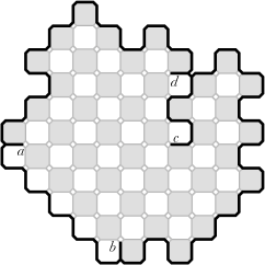
(a) A discrete domain with four marked boundary points. Marked points are the cusp points in the picture. The boundary of the discrete domain consists of four “admissible paths” (boundaries of chains of octagons and small squares alternating) on $\mathbb{L}^{\spadesuit}$.

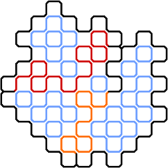
(b) In the 4 marked boundary points setting, a configuration of (the loop representation) of the FK Ising model consists of two interfaces and a number of loops. If $a,b,c,d$ are as on the figure (a), then the present configuration belongs to the internal arc configuration event ${(a\frown d,c\frown b)}$.

Figure 1. Discrete domain with 4 marked boundary points and a loop configuration on it.

Consider a domain $\Omega$ whose boundary is the outer boundary of a simple closed chain of faces where the octagons and the small squares are alternating. We assume that the “boundary conditions” change at 4 “marked” points, that is, the chain consist of exactly 4 open monochromatic chains of octagons and small squares. See Figure 1. The marked points are denoted by $a,b,c,d$ in general and we can assume they are the joint vertices of a black octagon, a white octagon and a small square in the chain and thus on the boundary of the domain. Assume that $a,b,c,d$ are counterclockwise ordered on the boundary and that the octagons next to the boundary arc $[ab]$ are white. Then necessarily the octagons next to $[cd]$ are white as well and the ones next to $[bc]$ or $[da]$ are black.

Let $G^{\spadesuit}\subset\mathbb{L}^{\spadesuit}$ be the graph which contains the vertices $(V(\mathbb{L}^{\spadesuit})\cap\Omega)\cup\{a,b,c,d\}$ and all the edges contained in $\Omega$. Let us consider a loop configuration which in the present case contains 2 open paths that both connect $\{a,c\}$ to $\{b,d\}$ and a number of closed loops. We assume that the configuration is dense on $G^{\spadesuit}$, in the sense that it covers all the vertices, and that the paths are simple and mutually disjoint. See Figure 1.

Define a probability measure on the dense simple loop configurations of $G^{\spadesuit}$ by requiring that the probability of a loop configuration is proportional to

$$\sqrt{2}^{(\#\textnormal{ of loops})}.$$ (1)

Notice that the number of open paths doesn’t enter this formula, since there are always 2 such paths. The model is called the loop representation of the critical FK Ising model (Fortuin–Kasteleyn random cluster model with a parameter value that corresponds to the Ising model).

1.1.1. The motivation of the FK random cluster model

The (spin) Ising model is a model for ferromagnetic substance. The Ising model configuration is a field of $\pm 1$ random variables, one on each vertex of a graph, and their probability law is given by the Boltzmann distribution of an energy functional with a nearest neighbor interaction. A parameter $\beta$ determines the strength of the interaction. The Fortuin–Kasteleyn random cluster model (FK model) is a percolation-type model with two parameter $p\in[0,1]$ and $q\geq 0$. The FK model configuration is a random subset of the set of edges of a graph. These edges are called open and the edge in the complement are called closed. A connected component (of vertices) in that random graph is called a cluster. In the FK model, the probability of the configuration is proportional to $q^{(\#\textnormal{ of clusters})}\,p^{(\#\textnormal{ of open edges})}\,(1-p)^{(\#\textnormal{ of closed edges})}$.

The FK Ising model is a particular case $q=2$ of the FK model. The spin Ising model and the FK Ising model are connected by the Edwards–Sokal coupling, that is, there exists a random field on the vertices and edges such that the marginal distribution of the random field on the vertices is the spin Ising model and the marginal distribution of the random field on the edges is the FK Ising model. For instance, spin correlations can be expressed in terms of connection probabilities using this coupling.

We consider only the case $q=2$ with the critical parameter $p=\frac{\sqrt{2}}{\sqrt{2}+1}$ in this article. Also we consider only the square lattice $\mathbb{Z}^{2}$, although, we could relax that assumption.

The loop representation of the random cluster configuration is a dense set of loops such that no loop intersects any open or dual-open edges (the loops are the boundaries of primal and dual clusters). The choice of critical parameter for the FK Ising random cluster model leads to the weight (1) for the loop representation.

1.2. Setting and notation for the scaling limit

1.2.1. Discrete setting, conditional measure and the scaling limit

For some $\delta>0$, $(\Omega_{\delta},a_{\delta},b_{\delta},c_{\delta},d_{\delta})$ be a simply connected discrete domain with four marked boundary points and lattice mesh $\delta>0$, that is, the boundary of $\Omega_{\delta}$ is a path on $\delta\mathbb{L}^{\spadesuit}$ with properties given above. We assume that the boundary arcs $\alpha_{1}=[a_{\delta}b_{\delta}]$, $\alpha_{2}=[b_{\delta}c_{\delta}]$, $\alpha_{3}=[c_{\delta},d_{\delta}]$ and $\alpha_{4}=[d_{\delta}a_{\delta}]$ are simple lattice paths on the modified medial lattice $\delta\mathbb{L}^{\spadesuit}$ such that the first and last edges are edges between two octagons and $\alpha_{1},\alpha_{2}^{\leftarrow},\alpha_{3},\alpha_{4}^{\leftarrow}$, where $\alpha^{\leftarrow}$ denotes the reversal of $\alpha$, have white octagons and small squares to their left and black octagons and white squares on their right.

Let $G_{\delta}$ be the graph on $\delta\mathbb{L}^{\bullet}$ corresponding to $\Omega_{\delta}$ and consider the FK model with wired boundary conditions on $[b_{\delta}c_{\delta}]$ and $[d_{\delta}a_{\delta}]$. Define also an enhanced graph $\hat{G}_{\delta}$ where we add the external arc pattern $(a_{\delta}\smile b_{\delta},c_{\delta}\smile d_{\delta})$ in the sense that the wired arcs are counted to be in the same component and in the weight (1), if the interface starting at $a_{\delta}$ ends at $b_{\delta}$, then it is counted as a closed loop.

There are two interfaces $\gamma$ and $\gamma^{*}$ starting at $a_{\delta}$ and $c_{\delta}$ respectively. Denote by $\mathbb{P}_{\delta}$ the probability law of $\gamma$ and by $\mathbb{P}_{\delta}^{+}$ the measure $\mathbb{P}_{\delta}$ conditional to the fact that $\gamma$ ends to $c_{\delta}$.

The scaling limits $\mathbb{P}=\lim_{\delta\to 0}\mathbb{P}_{\delta}$ and $\mathbb{P}^{+}=\lim_{\delta\to 0}\mathbb{P}_{\delta}^{+}$ are considered below.

1.2.2. Conformal transformation to the upper half-plane

It is useful to describe the probability laws in the upper-half plane (or in another fixed reference domain). We apply a conformal transformation such that the points $a_{\delta},b_{\delta},c_{\delta},d_{\delta}$ are mapped to points $U_{0}^{\delta},V_{0}^{\delta},W_{0}^{\delta},\infty$ respectively. Then $U_{0}^{\delta}<V_{0}^{\delta}<W_{0}^{\delta}$. As $\delta\to 0$, these points tend to some points $U_{0}<V_{0}<W_{0}$.

We will consider simple curves starting at $U_{0}$ as Loewner evolutions. In particular, we assume that they are parametrized by the half-plane capacity. The driving process is denoted by $U_{t}$ and three other marked points are $V_{t},W_{t}$ and $\infty$. In particular, $V_{t}$ and $W_{t}$ satisfy the Loewner equation driven by $U_{t}$. Then also $U_{t}<V_{t}<W_{t}$. Auxiliary processes are defined by setting

$$X_{t}=V_{t}-U_{t},\qquad Y_{t}=W_{t}-V_{t}.$$

1.3. The hypergeometric SLE$(\frac{16}{3})$

The hypergeometric SLE (see [18] and such processes also appear in [3, 12, 20]. Abbreviated to hSLE.) with parameter value $\kappa=\frac{16}{3}$ is defined by giving the driving process

$$\mathrm{d}U_{t} =\frac{4}{\sqrt{3}}\mathrm{d}B_{t}+\left(-\frac{2}{X_{t}}+\frac{2}{X_{t}+Y_{t}}-\frac{4}{3}\frac{Y_{t}\left(-1+\sqrt{1+\frac{X_{t}}{Y_{t}}}\right)}{X_{t}(X_{t}+Y_{t})}\right)\mathrm{d}t.$$ (2)

Note that the third term inside the brackets is equal to $-\frac{16}{3}\frac{F^{\prime}(z)}{F(z)}\frac{1-z}{s}$ evaluated at $z=\frac{X_{t}}{X_{t}+Y_{t}}$ and $s=X_{t}+Y_{t}$, where $F(z)$ is the hypergeometric function $\vphantom{F}{}_{2}F_{1}(\frac{3}{4},\frac{1}{4};\frac{3}{2};z)$.

1.4. The main result

By the results of [7], the scaling limit $\mathbb{P}=\lim_{\delta\to 0}\mathbb{P}_{\delta}$ is equal to a certain SLE$[\frac{16}{3},Z]$ process, that is, an SLE$(\frac{16}{3})$ process with a partition function $Z$. The topology of the convergence is given by the weak convergence of probability measures on the metric space of continuous functions. We use that result to prove the following theorem.

Theorem 1.1.

The sequence $\mathbb{P}_{\delta}^{+}$ converges, in the same topology as above, to $\mathbb{P}^{+}$ which is the law of a hypergeometric SLE$(\frac{16}{3})$.

See also Section 2.5 below for description of the scaling limit of the joint law of the pair $(\gamma,\gamma^{*})$.

2. Scaling limit of FK Ising model interface as hyperbolic SLE

2.1. Discrete martingale observable

In the random cluster model we take the boundary conditions which are free–wired–free–wired and they change across the edges corresponding to $a_{\delta},b_{\delta},c_{\delta},d_{\delta}$. There are interfaces starting and ending to these points. Due to topological (as well as parity) reasons, the interface starting at $a_{\delta}$ has to end at $b_{\delta}$ or $d_{\delta}$. We denote these two mutually exclusive events as $(a_{\delta}\frown b_{\delta},c_{\delta}\frown d_{\delta})$ and $(a_{\delta}\frown d_{\delta},c_{\delta}\frown b_{\delta})$, respectively, and we call them internal arc patterns.

We consider the quantity

$$M_{t}^{\delta}=\mathbb{P}_{\delta}(\,(a_{\delta}\frown d_{\delta},c_{\delta}\frown b_{\delta})\,|\,\mathcal{F}_{t})$$ (3)

which we call an observable. Here $\mathcal{F}_{t}$ is the $\sigma$-algebra generated by $\gamma(s)$, $s\in[0,t]$. Since $M_{t}^{\delta}$ is a conditional expected value of a random variable with respect to $\mathcal{F}_{t}$, the process $(M_{t}^{\delta})_{t\geq 0}$ is a martingale with respect to the filtration $(\mathcal{F}_{t})_{t\geq 0}$ and the probability measure $\mathbb{P}_{\delta}$.

2.2. Scaling limit of the observable

In [7], it was shown that the observables $M_{t}^{\delta}$ converge to a scaling limit $M_{t}$. It has an explicit formula

$$M_{t}=\sqrt{1+\frac{Y_{t}}{X_{t}}}-\sqrt{\frac{Y_{t}}{X_{t}}}.$$ (4)

The mode of convergence is given by the following result:

Proposition 2.1.

For each $\varepsilon>0$ and $T>0$, there exists an event $E$ and $\delta_{0}>0$ such that the following holds. If $\delta\leq\delta_{0}$, then $\mathbb{P}_{\delta}(E)>1-\varepsilon$ and

$$\sup_{E}\sup_{t\in[0,T]}|M_{t}^{\delta}-M_{t}|\leq\varepsilon.$$

It follows that also $M_{t}$ is a martingale. Namely, let $s<t$ and let $f$ be any continuous, bounded random variable which is measurable with respect to $\mathcal{F}_{s}$. Then $\mathbb{E}_{\delta}(M_{t}^{\delta}f)=\mathbb{E}_{\delta}(M_{s}^{\delta}f)$ by the martingale property of the discrete observable. By the triangle inequality

$$|\mathbb{E}(M_{t}f)-\mathbb{E}(M_{s}f)|\leq \;|\mathbb{E}(M_{t}f)-\mathbb{E}_{\delta}(M_{t}f)|+|\mathbb{E}(M_{s}f)-\mathbb{E}_{\delta}(M_{s}f)|$$

$$+|\mathbb{E}_{\delta}((M_{t}-M_{t}^{\delta})f)|+|\mathbb{E}_{\delta}((M_{s}-M_{s}^{\delta})f)|.$$

First and second term tend to zero as $\delta\to 0$ by the weak convergence of probability measures. The third and fourth term also tend to zero by Proposition 2.1, since $|\mathbb{E}_{\delta}((M_{t}-M_{t}^{\delta})f)|\leq 2\,\mathbb{E}_{\delta}(\mathbbm{1}_{E^{c}}|f|)+\sup_{E}\sup_{t\in[0,T]}\;|M_{t}^{\delta}-M_{t}|\,\mathbb{E}_{\delta}(|f|)$.

2.3. Weighting by a martingale

We weight the probability measure by the martingale $M_{t}/M_{0}$ (the process is stopped upon the martingale hitting $0$ or $1$, i.e. when $X_{t}$ or $Y_{t}$ hit zero).

Denote the event $(a_{\delta}\frown d_{\delta},c_{\delta}\frown b_{\delta})$ by $A$. Then by properties of conditional expected values

$$\mathbb{E}(fM_{t})=\mathbb{E}(f\,\mathbb{E}(\mathbbm{1}_{A}\,|\,\mathcal{F}_{t}))=\mathbb{E}(\mathbb{E}(f\,\mathbbm{1}_{A}\,|\,\mathcal{F}_{t}))=E(f\,\mathbbm{1}_{A})$$

for any $\mathcal{F}_{t}$-measurable bounded random variable $f$. Thus the probability measure $\mathbb{P}$ weighted by $M_{t}/M_{0}$ can be interpreted as to be conditioned by the event ${(a_{\delta}\frown d_{\delta},c_{\delta}\frown b_{\delta})}$ and thus equals to $\mathbb{P}^{+}$.

2.3.1. Girsanov’s theorem

Suppose that $N_{t}$ is a martingale such that

$$M_{t}=\exp\left(N_{t}-\frac{1}{2}\langle N\rangle_{t}\right)$$

Then by Itô’s lemma, $M_{t}$ and $N_{t}$ satisfy the identity

$$N_{t}=N_{0}+\int_{0}^{t}\frac{\mathrm{d}M_{s}}{M_{s}}$$

which can be used for defining $N_{t}$ for any positive martingale $M_{t}$.

Under the probability measure weighted by the martingale $M_{t}/M_{0}$, it holds that the process

$$B_{t}-\langle B,N\rangle_{t}$$ (5)

is a standard Brownian motion by Girsanov’s theorem (see for instance [5], Section 2.12). Thus if we have a Loewner evolution whose driving process is

$$U_{t}=U_{0}+\sqrt{\kappa}B_{t}+D_{t}$$

where $D_{t}$ is the drift of $W_{t}$ in the sense that $D_{t}$ is a bounded variation process, then the driving process can be written as

$$U_{t}=U_{0}+\sqrt{\kappa}\hat{B}_{t}+D_{t}+\Delta_{t}$$

where $\hat{B}_{t}$ is a standard Brownian motion under the weighted probability measure. Here

$$\Delta_{t}=\sqrt{\kappa}\langle B,N\rangle_{t}$$

by (5).

2.4. The driving process conditioned on the internal arc configuration

Remember that by results in [7],

$$M_{t}=M_{0}+\int_{0}^{t}\frac{1}{2\sqrt{3}}\frac{(1-M_{s}^{2})^{3}}{Y_{s}\,M_{s}(M_{s}^{2}+1)}\mathrm{d}B_{s}$$

and

$$\mathrm{d}U_{t}=-\frac{4}{\sqrt{3}}\mathrm{d}B_{t}+\left(\frac{2}{X_{t}}-\frac{1}{3}\frac{(3M_{t}^{4}+2M_{t}^{2}+1)(1-M_{t}^{2})^{2}}{Y_{t}M_{t}^{2}(M_{t}^{2}+1)^{2}}\right)\mathrm{d}t.$$

Consequently by the considerations of Section 2.3.1, for a process $(\hat{B}_{t})$ which is a Brownian motion under the measure $\mathbb{P}^{+}$ (the one weighted by $(M_{t}/M_{0})$), it holds that

$$\mathrm{d}U_{t} =-\frac{4}{\sqrt{3}}\mathrm{d}\hat{B}_{t}+\left(\frac{2}{X_{t}}-\frac{1}{3}\frac{(3M_{t}^{4}+2M_{t}^{2}+1)(1-M_{t}^{2})^{2}}{Y_{t}M_{t}^{2}(M_{t}^{2}+1)^{2}}-\frac{2}{3}\frac{(1-M_{s}^{2})^{3}}{Y_{s}\,M_{s}^{2}(M_{s}^{2}+1)}\right)\mathrm{d}t$$

$$=-\frac{4}{\sqrt{3}}\mathrm{d}\hat{B}_{t}+\left(\frac{2}{X_{t}}-\frac{1}{3}\frac{(M_{t}^{4}+2M_{t}^{2}+3)(1-M_{t}^{2})^{2}}{Y_{t}M_{t}^{2}(M_{t}^{2}+1)^{2}}\right)\mathrm{d}t.$$

The rightmost term on the first line is $\sqrt{\kappa}\,\mathrm{d}\langle B,N\rangle_{t}$. By plugging in the expression (4) gives after some algebra

$$\mathrm{d}U_{t} =-\frac{4}{\sqrt{3}}\mathrm{d}\hat{B}_{t}+\left(\frac{2}{X_{t}}-\frac{2}{X_{t}+Y_{t}}-\frac{4}{3}\frac{Y_{t}\left(2+\sqrt{1+\frac{X_{t}}{Y_{t}}}\right)}{X_{t}(X_{t}+Y_{t})}\right)\mathrm{d}t$$

which is equivalent to (2). Thus it follows that $\mathbb{P}^{+}$ is the law of a hypergeometric SLE$(\frac{16}{3})$.

2.5. Joint law of the pair of interfaces in the arc configuration

The scaling limit of the joint law of the interfaces from $a_{\delta}$ to $d_{\delta}$ and $c_{\delta}$ to $b_{\delta}$ under the probability measure conditioned on the event $(a_{\delta}\frown d_{\delta},c_{\delta}\frown b_{\delta})$ can be characterized in the following way.

Consider the scaling limit of the pair of interfaces in the conditioned arc configuration after conformal transformation to the upper half-plane and let the curves be $\gamma_{1}$ and $\gamma_{2}$ such that $\gamma_{1}$ and $\gamma_{2}$ start at $U_{0}$ and $W_{0}$, respectively. Parametrize the curves $\gamma_{1}$ and $\gamma_{2}$ in some way. For instance, use the half-plane capacity seen from $\infty$ or $V_{0}$ as parametrization for $\gamma_{1}$ and $\gamma_{2}$, respectively. Then define $\mathcal{F}_{s,t}$ to be the $\sigma$-algebra generated by $\gamma_{1}(q)$, $q\in[0,s]$, and $\gamma_{2}(r)$, $r\in[0,t]$.

By the same argument that says that the marginal law of $\gamma_{1}$ is the hSLE, we see that conditionally on $\mathcal{F}_{s,t}$, the marginal law of $\gamma_{1}$ is the hSLE. Degenerate versions of these statements give that (i) the pair $(\gamma_{1},\gamma_{2})$ can be sampled by sampling first $\gamma_{j}$, $j=1$ or $2$, as hSLE in $\mathbb{H}$ and then sampling $\gamma_{3-j}$ in $H$, where $H$ is the component of $\gamma_{3-j}(0)+\mathrm{i}\,(0+)$ in $\mathbb{H}\setminus\gamma_{j}(0,\infty)$, as an independent chordal SLE and $(ii)$ that a similar conditional version holds (i.e. conditional on $\mathcal{F}_{s,t}$, the pair can be sampled as an hSLE and an independent chordal SLE).

3. Comparison to a similar result on percolation

Let us compare the previous case of FK Ising model to that of the critical site percolation model on triangular lattice.

Consider the site percolation model on the triangular lattice

$${\delta L_{\textnormal{tri}}}={\{\delta(j+ke^{\mathrm{i}\pi/3})\,:\,j,k\in\mathbb{Z}\}}.$$

It was shown in [14], that the interface of this model in the chordal setup converges to SLE$(6)$.

Note that the existence of an open percolation crossing from $[a_{\delta}b_{\delta}]$ to $[c_{\delta}d_{\delta}]$ in $\Omega_{\delta}$ is exactly the event of an internal arc pattern $(a_{\delta}\frown d_{\delta},c_{\delta}\frown b_{\delta})$ of interfaces. A central result in [14] is that the probability of such a crossing event is given by Cardy’s formula

$$\lim_{\delta\to 0}\mathbb{P}_{\delta}((a_{\delta}\frown d_{\delta},c_{\delta}\frown b_{\delta}))=C\,\left(\frac{X_{0}}{X_{0}+Y_{0}}\right)^{\frac{1}{3}}\,\vphantom{F}_{2}F_{1}\left(\frac{1}{3},\frac{2}{3},\frac{4}{3};\frac{X_{0}}{X_{0}+Y_{0}}\right)$$

holds, where $X_{0}=V_{0}-U_{0}$ and $Y_{0}=W_{0}-V_{0}$ with the notation used above and $C$ is a constant, whose exact value we don’t need below.

It follows then that

$$M_{t}=\left(\frac{X_{t}}{X_{t}+Y_{t}}\right)^{\frac{1}{3}}\,\vphantom{F}_{2}F_{1}\left(\frac{1}{3},\frac{2}{3},\frac{4}{3};\frac{X_{t}}{X_{t}+Y_{t}}\right)$$

is a martingale for the scaling limit for $t\leq\tau$ where $\tau$ is the time when the quarilateral degenerates (the interface hits $[bc]$ or $[cd]$). Since the interface (exploration process from $a$ to $d$) converges to the chordal SLE$(6)$,

$$\mathrm{d}U_{t}=\sqrt{6}\,\mathrm{d}B_{t},\qquad\mathrm{d}X_{t}=-\sqrt{6}\,\mathrm{d}B_{t}+\frac{2}{X_{t}},\qquad\partial_{t}Y_{t}=\frac{2}{X_{t}+Y_{t}}-\frac{2}{X_{t}}.$$

Thus it follows that if $\mathrm{d}N_{t}=\frac{\mathrm{d}M_{t}}{M_{t}}$

$$\sqrt{6}\,\mathrm{d}\langle B,N\rangle_{t}=-\frac{2\left(\frac{Y_{t}}{X_{t}+Y_{t}}\right)^{\frac{1}{3}}}{X_{t}\,\vphantom{F}{}_{2}F_{1}\left(\frac{1}{3},\frac{2}{3},\frac{4}{3};\frac{X_{t}}{X_{t}+Y_{t}}\right)}\mathrm{d}t$$

Thus for the process $\hat{B}_{t}=B_{t}-\langle B,N\rangle_{t}$ which is a Brownian motion under the probability measure weighted by the martingale $M_{t}/M_{0}$, the driving process $U_{t}$ satisfies

$$\mathrm{d}U_{t} =\sqrt{6}\mathrm{d}\hat{B}_{t}-\frac{2\left(\frac{Y_{t}}{X_{t}+Y_{t}}\right)^{\frac{1}{3}}}{X_{t}\,\vphantom{F}{}_{2}F_{1}\left(\frac{1}{3},\frac{2}{3},\frac{4}{3};\frac{X_{t}}{X_{t}+Y_{t}}\right)}\mathrm{d}t$$

which shows that the Loewner evolution is the hypergeometric SLE$(6)$.

References

• [1] M. Bauer, D. Bernard, and K. Kytölä. Multiple Schramm–Loewner Evolutions and Statistical Mechanics Martingales. Journal of Statistical Physics, 120(5-6):1125–1163, Sept. 2005.
• [2] J. Dubedat. SLE($\kappa$, $\rho$) martingales and duality. Annals of probability, 33(1):223–243, Jan. 2005.
• [3] J. Dubedat. Euler integrals for commuting SLEs. Journal of Statistical Physics, 123(6):1183–1218, June 2006.
• [4] J. Dubedat. Commutation relations for Schramm-Loewner evolutions. Communications on Pure and Applied Mathematics, 60(12):1792–1847, Dec. 2007.
• [5] R. Durrett. Stochastic calculus. Probability and Stochastics Series. CRC Press, Boca Raton, FL, 1996.
• [6] K. Izyurov. Critical Ising interfaces in multiply-connected domains. Probability Theory and Related Fields, 167(1-2):379–415, Feb. 2017.
• [7] A. Kemppainen and S. Smirnov. Conformal invariance of boundary touching loops of FK Ising model. arXiv.org, page arXiv:1509.08858, Sept. 2015, 1509.08858.
• [8] A. Kemppainen and S. Smirnov. Conformal invariance in random cluster models. II. Full scaling limit as a branching SLE. arXiv.org, page arXiv:1609.08527, Sept. 2016, 1609.08527.
• [9] G. Lawler. Schramm-Loewner evolution (SLE). In Statistical mechanics, pages 231–295. Amer. Math. Soc., Providence, RI, 2009.
• [10] G. Lawler, O. Schramm, and W. Werner. Conformal restriction: the chordal case. Journal of the American Mathematical Society, 16(4):917–955 (electronic), 2003.
• [11] G. F. Lawler. Partition Functions, Loop Measure, and Versions of SLE. Journal of Statistical Physics, 134(5-6):813–837, Mar. 2009.
• [12] W. Qian. Conformal restriction: The trichordal case. arXiv.org, Feb. 2016, 1602.03416v1.
• [13] O. Schramm. Scaling limits of loop-erased random walks and uniform spanning trees. Israel Journal of Mathematics, 118(1):221–288, 2000.
• [14] S. Smirnov. Critical percolation in the plane: conformal invariance, Cardy’s formula, scaling limits. Comptes Rendus de l’Académie des Sciences. Série I. Mathématique, 333(3):239–244, 2001.
• [15] S. Smirnov. Critical percolation in the plane. arXiv.org, Sept. 2009, 0909.4499v1.
• [16] S. Smirnov. Conformal invariance in random cluster models. I. Holomorphic fermions in the Ising model. Annals of Mathematics. Second Series, 172(2):1435–1467, 2010.
• [17] W. Werner. Girsanov’s transformation for SLE($\kappa$,$\rho$) processes, intersection exponents and hiding exponents. Annales de la Faculté des Sciences de Toulouse. Mathématiques. Série 6, 13(1):121–147, 2004.
• [18] H. Wu. Convergence of the Critical Planar Ising Interfaces to Hypergeometric SLE. arXiv.org, Oct. 2016, 1610.06113v3.
• [19] D. Zhan. The scaling limits of planar LERW in finitely connected domains. The Annals of Probability, 36(2):467–529, Mar. 2008.
• [20] D. Zhan. Reversibility of Some Chordal SLE(kappa;rho) Traces. Journal of Statistical Physics, 139(6):1013–1032, June 2010.