The shortest periodic and flaring flux variability of a methanol maser emission at 6.7 GHz in G 014.23$-$00.50

Abstract

We detected flaring flux variability that regularly occurred with the period of 23.9 days on a 6.7 GHz methanol maser emission at $V_{\mathrm{lsr}}=$ 25.30 km s^-1 in G 014.23$-$00.50 through highly frequent monitoring using the Hitachi 32-m radio telescope. By analyzing data from 05 January 2013 to 21 January 2016, the periodic variability has persisted in at least 47 cycles, corresponding to $\sim$1,100 days. The period of 23.9 days is the shortest one observed in masers at around high-mass young stellar objects so far. The flaring component normally falls below the detection limit (3$\sigma$) of $\sim$0.9 Jy. In the flaring periods, the component rises above the detection limit with the ratio of the peak flux density more than 180 in comparison with a quiescent phase, showing intermittent periodic variability. The time-scale of the flux rise was typically two days or shorter, and both symmetric and asymmetric profiles of flux variability were observed through intraday monitoring. These characteristics might be explained by a change in the flux of seed photons by a colliding-wind binary (CWB) system or a variation of the dust temperature by an extra heating source of a shock formed by the CWB system within a gap region in a circumbinary disk, in which the orbital semi-major axes of the binary are 0.26–0.34 au.

1 Introduction

Periodic flux variability of the methanol masers was first discovered in G 009.62$+$00.19 E, i.e., periodic variability with the interval of 246 days ([Goedhart et al. (2003)]; modified to $243.3\pm 2.1$ days in [Goedhart et al. (2014)]). So far, the periodic flux variability of the methanol masers has been detected in 20 sources (including quasi-periodic ones). Their periods range from 29.5 to 668 days ([Goedhart et al. (2004)], goedhart09; [Araya et al. (2010)]; [Szymczak et al. (2011)], szymczak14, szymczak15, szymczak16; [Fujisawa et al. (2014a)]; [Maswanganye et al. (2015)], maswan16). Patterns of the variability have been classified into two categories: the sinusoidal one, and the intermittent one with a quiescent phase. Such periodic flux variability was also observed in other masers, i.e., silicon monoxide in Orion Kleinmann-Low (KL) (Ukita et al., 1981), formaldehyde in IRAS 18556$+$0408 (Araya et al., 2010), hydroxyl in G 012.88$+$00.48 (Green et al., 2012a), and water in IRAS 22198$+$6336 (Szymczak et al., 2016), and variations of these lines except for the silicon monoxide were synchronized with the variations of methanol masers in the same sources. The periodic variability, therefore, must be a common phenomenon at around high-mass (proto-)stars, but appears in limited conditions. Because of their short timescale, the periodic variability is potentially important in studying high-mass protostars and their circumstellar structure on spatial scales of 0.1–1 au, which are estimated under the condition of Keplerian rotation.

Four models have been proposed for interpretations of the periodic flux variability, in the point of view that variations of (multiple) spectral components are synchronized with 1–14 days’ delay in some sources, possibly caused by global variation on a central engine: a colliding-wind binary (CWB: van der Walt et al. (2009); van der Walt (2011)), a stellar pulsation (Inayoshi et al. (2013); Sanna et al. (2015)), a circumbinary accretion disk (Araya et al., 2010), and a rotation of spiral shocks within a gap region in a circumbinary disk (Parfenov & Sobolev, 2014). The first model is based on changes in the flux of seed photons, while the remaining three ones are based on changes in the temperature of dust grains at the masing regions.

Long-term and frequent flux monitoring was conducted toward source samples only less than 20%, which was estimated from $\sim$200 sources (e.g., Goedhart et al. (2004); Szymczak et al. szymczak15; Maswanganye et al. (2016)) in more than 1000 methanol masers samples (e.g., Pestalozzi et al. (2005); Xu et al. (2009); Caswell et al. (2010), caswell11; Green et al. (2010), green12b; Olmi et al. (2014); Sun et al. (2014); Breen et al. (2015), and references therein). Furthermore, most of the monitored sources have been selected simply by their peak flux densities $>$ 5 Jy in Szymczak, Wolak, and Bartkiewicz (2015). We initiated a long-term, highly frequent, and unbiased monitoring project using the Hitachi 32-m radio telescope (Yonekura et al., 2016) on 30 December 2012 toward a large sample of the 6.7 GHz methanol masers (442 sources) that are located in declination $>$ -30D. The observations have been carried out daily, monitoring a spectrum of each source with intervals of 9–10 days. The detailed results of this project will be reported in forthcoming papers. In this paper, we focus on remarkable flux variability detected in the 6.7 GHz methanol masers associated with G 014.23$-$00.50 (hereafter G 014.23).

The 6.7 GHz methanol maser emission in G 014.23 was discovered by the methanol multibeam survey toward the galactic longitude 6-20D (Green et al., 2010). G 014.23 is located in the infrared dark cloud (IRDC) G 14.225$-$00.506, which is first identified by Peretto and Fuller (2009) as a proto-OB association (Povich & Whitney, 2010). This IRDC, also recognized as M17 SWex (Povich & Whitney, 2010), is part of extended ($\sim 80$ pc $\times$ $20$ pc) and massive ($>10^{5}$ ) molecular clouds discovered by Elmegreen and Lada (1976) and is located at the southwest of the Galactic HII region M17. The distance to M17 has been estimated to be 1.98${}^{+0.14}_{-0.12}$ kpc through trigonometric parallaxes of the methanol masers (Xu et al., 2011). Systemic velocities of M17 and M17 SWex are the same within $\sim$1 km s^-1 in the line emissions of HCO⁺, N₂H⁺ ($V_{\mathrm{lsr}}\sim 18.5$–19.5 km s^-1: Schlingman et al. (2011); Shirley et al. (2013)) and the absorption of H₂CO ($V_{\mathrm{lsr}}\sim 19$–20 km s^-1: Sewilo et al. (2004); Okoh et al. (2014)). Based on these results, we adopt the distance of G 014.23 to be 2 kpc in this paper. The methanol maser emission is detected at “Hub-N”, a denser dust region where two filaments intersect within the size of $\sim$1 pc (Busquet et al., 2013) and the total mass of $\sim$10³ (Busquet et al., 2016). This region exhibits signs of active star formation, such as higher temperature in NH₃ line emissions ($T_{\mathrm{rot}}\sim 15$ K) and larger non-thermal velocity dispersion ($\sigma_{\mathrm{NT}}\sim 1$ km s^-1) than those of the filaments in other regions ($T_{\mathrm{rot}}\sim 11$ K, $\sigma_{\mathrm{NT}}\sim 0.6$ km s^-1) (Busquet et al., 2013).

Among the five-times observations toward G 014.23 by Green et al. (2010), the methanol masers were detected only twice, being interpreted as flaring in flux variations. The water maser emission at 22.2 GHz was also detected in the same dusty area Hub-N in the IRDC G 14.225$-$00.506 (Wang et al., 2006). Figure 1 shows the methanol and water masers positions superposed on the dust emission at $\lambda=1.3$ mm obtained using the submillimeter array (SMA: Busquet et al. (2016)), with the positions of pre/proto-stellar cores identified using the atacama large millimeter/submillimeter array (ALMA) at $\lambda=3$ mm (Ohashi et al., 2016) and young stellar objects (YSOs) identified by Povich and Whitney (povich10). In the high-resolution observations using the SMA, the water masers are presented as being associated with the brightest dust condensation MM1a with the mass of $\sim$13 , while in the ALMA observation the methanol masers are associated with a proto-stellar core with the mass of $\sim$13 . The proto-stellar core includes an intermediate-mass YSO G014.2300$-$00.5097 (Povich & Whitney (2010): $\sim 10^{2}$ , 3.3 ). This intermediate-mass YSO is classified as the stage 0/I according to the definition by Robitaille et al. (2006), suggesting that infalling activities from a surrounding envelope are still dominant. Furthermore, an excess in 4.5 $\micron$ band is also detected at this intermediate-mass YSO, and it might be due to unresolved analogs of the extended green objects, which are candidates of active outflows ejected from high-mass YSOs at an early evolutionary phase (Cyganowski et al., 2008). These characteristics imply that this intermediate-mass YSO accompanied by the methanol masers is a precursor of a B-type star on the main sequence (Povich & Whitney, 2010).

In this paper, we discuss remarkable flux variability detected in the 6.7 GHz methanol masers of G 014.23. The structure of this paper is as follows: in sections 2 and 3, we present observations and results with data reduction for determination of periods, respectively. In section 4, we discuss suitable models to explain the remarkable flux variability.

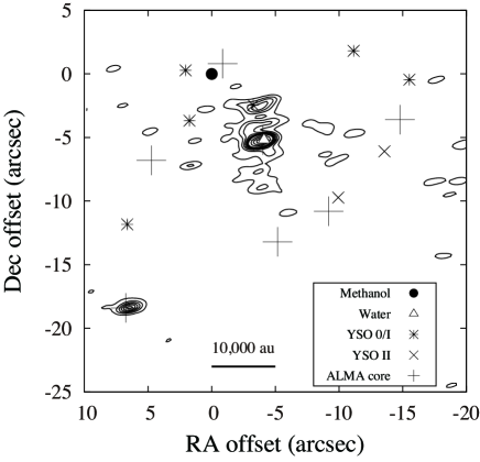
Figure 1: Close-up map of the 6.7 GHz methanol maser position (filled circle) in the dense dust region “Hub-N” in G 014.23. The origin of the map corresponds to the absolute position of the methanol maser emission at the local standard of rest (LSR) velocity $V_{\mathrm{lsr}}=25.3$ km s^-1 [$\alpha$(J2000.0) = 18h18m12s.59, $\delta$(J2000.0) = -16D49’22”.8] (Green et al. (2010): positional uncertainty of $\sim$0”.4). The linear spatial scale is shown by the ruler at the bottom. The 22.2 GHz water masers (Wang et al. (2006): blank triangle) and YSOs identified as the evolutionary stage 0/I (asterisk) and II (cross) by Povich and Whitney (povich10) are shown in the map. Their positional uncertainties were $\sim$0”.01 and $\sim$0”.3. The masers and YSOs are superposed on the contour map of the dust emission at 1.3 mm obtained using the SMA (Busquet et al., 2016), which is represented with the same contour levels used in the right panel of their figure 2 (from 3 to 21$\sigma$ in steps of 3$\sigma$, and from 21 to 51$\sigma$ in steps of 10$\sigma$, where $\sigma$ is the rms of the map 1 mJy beam^-1). Their synthesized beam is 1”.46$\times$0”.46 (position angle of -78D), and their positional uncertainties are less than 1”. The peak positions of pre/proto-stellar cores identified using the ALMA at 3 mm (Ohashi et al., 2016) are shown by large crosses (the synthesized beam of 3”.7$\times$2”.0 ).

2 Observations

2.1 Periodic monitoring at 10-day intervals

Time range of the periodic flux monitoring using the Hitachi 32-m radio telescope. Period Time range of monitoring A.D. MJD [yyyy/mm/dd] [day] Periodic monitoring at 10-day intervals 2013/01/05 – 2014/01/10 56297 – 56667 Daily monitoring 2014/05/07 – 2016/01/21 56784 – 57408 Intraday monitoring 0 2014/03/29 – 2014/05/01 56745 – 56778 I 2015/08/09 – 2015/08/19 57243 – 57253 II 2015/09/01 – 2015/09/16 57266 – 57281 III 2015/09/30 – 2015/10/04 57295 – 57299 IV 2015/10/26 – 2015/10/31 57321 – 57326 Column 1: Identification number for intraday monitoring; Columns 2, 3: Time range of each periodic flux monitoring as A.D. and modified julian day.

We made flux monitoring with intervals of 9–10 days, the time range of which is listed in table 2.1, using the Hitachi 32-m radio telescope toward the target source G 014.23. The full-width at half maximum (FWHM) of the beam is 4.6’ and the pointing accuracy is better than 30”. Each observation was made at almost the same azimuth and elevation angles (169D, 35D) to minimize the effects of pointing errors for observed flux densities. Left-circular polarization (LCP) signals were recorded on hard disk drive by using the 64 Mbps mode (16 mega-samples per second with 4 bit sampling) through K5/VSSP32 sampler and converted to spectra using software spectroscopic system (Nitsuki 9270: Kondo et al. (2008)). The bandwidth is 8 MHz (RF: 6664–6672 MHz), covering the velocity range of $\sim$360 km s^-1. The number of frequency channels is originally 2,097,152, but they are bunched into 8,192 channels, yielding the velocity resolution of 0.044 km s^-1. The system noise temperature at the zenith after the correction for the atmosphere opacity ($T_{\mathrm{sys}}^{\ast}$) and the aperture efficiency ($\eta_{\mathrm{A}}$) is typically 30–40 K and 55–75% at 6.7 GHz, respectively. The rms noise level (1$\sigma$) is achieved to be $\sim$0.3 Jy with an integration time of 5 min and further 3 ch smoothing, yielding the velocity resolution of 0.13 km s^-1. The antenna temperature ($T_{\mathrm{a}}^{\ast}$) was measured by the chopper-wheel method. We observed a sky area (+60’ offset in right ascension direction) as off-source data just after each on-source scan in the $T_{\mathrm{a}}^{\ast}$ measurement.

2.2 Daily monitoring

We initiated daily monitoring on 7 May 2014 (modified julian day (MJD) $=$ 56784) with the same observational setup as that described in section 2.1. The time range of the daily monitoring is listed in table 2.1. During this observation period, there are blank dates when the daily monitoring was not made due to system maintenance or other observations as follows: 9–20 June and 12–27 July 2014 (MJD 56817–56828 and 56850–56865, respectively), and 25 May to 6 June and 20–31 August 2015 (MJD 57167–57179 and 57254–57265, respectively). The stability of the system was evaluated by daily monitoring of the 6.7 GHz methanol masers in G 012.02$-$00.03 and G 069.52$-$00.97 (Onsala 1) in the same periods. Their peak flux densities were stronger than 100 Jy and stable whose variations were smaller than 10% during the periods. The variations were estimated from the modulation index expressed as the standard deviation normalized by the averaged value of flux densities in each source. As a result, the stability of the observational system is estimated to be better than 15%.

2.3 Intraday monitoring

We carried out intraday monitoring in five epochs (table 2.1) with the same observational setup as that described in section 2.1, except for the azimuth and elevation angles. The intraday monitoring is classified into the periods 0 and I–IV; the former was made before an evaluation of the periodicity while the latter were made after the evaluation. In the period 0 in 2014, we focused on investigating whether there occurred flux variations weaker than 0.9 Jy, which was equal to the detection limit (3$\sigma$) with the integration time of 5 min. The observational cycle of 10.5 min that consists of 5 min for the target source, half a minute for slewing, and 5 min for the off source was repeated during the elevation angles $\gtrsim$ 30D until 27 April (MJD 56774) and $\geq$ 15D from 28 April (MJD 56775). The detection limits of 3$\sigma=$ 0.15–0.20 Jy were achieved in each observational day by integrating all the scans. On the other hand, in the periods I–IV in 2015, we focused on measuring accurate time-scale of rises and decays of flux densities and profiles of flux variations during each period. The maser G 014.10$+$00.08 was used as a calibrator, located close to the target with the separation angle of 36.6’. Its peak flux densities were 70–80 Jy and stable whose variation was smaller than 10% during each period. The cycle consisting of $\sim$11 min single-point observation of G 014.23 (5 min on-source and 5 min off-source) and $\sim$15 min nine-point cross-scan of G 014.10$+$00.08 was repeated during the elevation angles $\geq$ 15D to calibrate pointing errors and atmospheric effects. Solutions for the calibration obtained within two to three days at the beginning of each period were applied to all the data during the periods.

3 Results

First of all, we made an average spectrum of G 014.23 by integrating all observational data to identify spectral components, as shown in figure 2. This average was weighted by $\sigma^{-2}$, an inverse square of rms noise level. From the intraday monitoring described in section 2.3, we picked up one 5-min scan for each day observed at the same azimuth and elevation angles (169D, 35D) as the periodic monitoring in section 2.1 and 2.2. This procedure provides us with a chance for handling all the data equally without being biased toward data during flares. As a result, the average spectrum was obtained from 504 scans of 5 min duration, or 42 hrs (2,520 min) integration time in total, achieving the detection limit as 3$\sigma$ of 0.039 Jy. In this spectrum, five spectral components were identified at $V_{\mathrm{lsr}}=$ 22.30, 23.46, 23.91, 24.69, and 25.30 km s^-1. In addition, two spectral components at $V_{\mathrm{lsr}}=$ 20.98 and 21.75 km s^-1 were identified in limited periods of the monitoring (see section 3.1). These are labeled as A, B, C, D, E, F, and G, respectively in order of velocity. The six components A–F are newly detected. The significant dip of $\sim$0.05 Jy was detected at $V_{\mathrm{lsr}}\sim$19–20 km s^-1 and could be an absorption line because of $V_{\mathrm{lsr}}$ close to one of H₂CO absorption line (Sewilo et al., 2004). However, it is beyond the scope of this paper.

3.1 Flux variability

Figure 3 shows time variations of flux densities of all spectral components from 5 January 2013 to 21 January 2016 (MJD 56297–57408). Concerning the data points during the intraday monitoring, only the results measured at the same azimuth and elevation angles as the periodic monitoring are shown in figure 3.

The component G showed remarkable variability (filled circle in figure 3). The flux density of this component in a quiescent phase is usually below the detection limit of $\sim$0.9 Jy. This component, however, sometimes rises above the detection limit. The time-scale of the rise is two days or shorter in most cases, and the component decays within a few days, which could be called a “flare.” Figure 4 shows representative spectra as a typical case for the flaring activities. There was no emission in the top panel observed on MJD 57105, and the component G was detected on the next day (MJD 57106) shown in the middle panel, while it disappeared three days later (MJD 57109) in the bottom panel. We have detected clear periodicity in this component, as described in detail in section 3.2.

The components A–F emerged on MJD 56788 (11 May 2014) and showed flux variations until MJD 57130 (18 April 2015). In particular, three components C, D, and E (asterisk, blank diamond, and filled diamond in the upper-panel of figure 3) showed notable flux variations until MJD 56943, which were brighter than the maximum flux density of the flaring component G. The time-scale of the variations was longer than 100 days. No correlation was seen between the long-term flux variability of the components A–F and the flaring activities of the component G. The maximum flux density of the component G during our monitoring was detected after the period when the components A–F were bright, suggesting also that those have poor correlation. In this paper, we mainly focus on the flaring activities of the component G.

Figure 2: Average spectrum of the 6.7 GHz methanol maser emission in G 014.23. All 504 scans of 5 min duration obtained at the same azimuth (169D) and elevation (35D) angles were used. This average was weighted by $\sigma^{-2}$ (inverse square of rms noise level), and the 3$\sigma$ detection limit of 0.039 Jy was achieved. Labels A, B, C, D, E, F, and G indicate spectral components at $V_{\mathrm{lsr}}=$ 20.98, 21.75, 22.30, 23.46, 23.91, 24.69, and 25.30 km s^-1, respectively. Note that the components A and B do not fulfill the 3$\sigma$ criterion to be real in this figure.

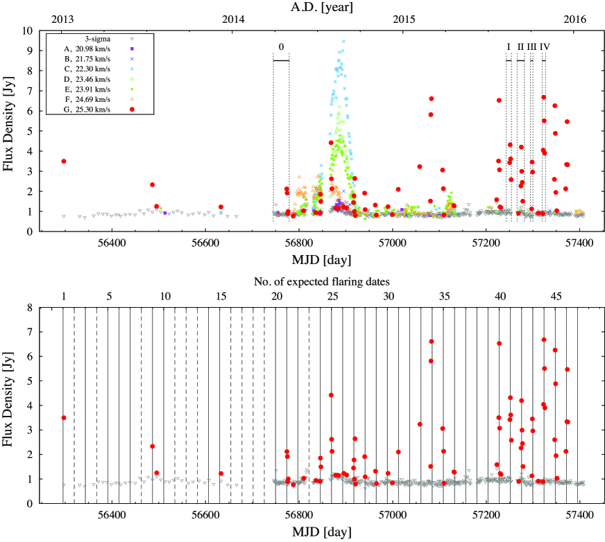
Figure 3: Upper-panel: Flux variation of each spectral component of the 6.7 GHz methanol masers in G 014.23 from 5 January 2013 to 21 January 2016 (MJD 56297–57408). Each symbol shows the spectral components referred as legends at top-left corner. The time intervals denoted by dotted vertical lines correspond to the periods of the intraday flux monitoring 0–IV, as described in section 2.3. Lower-panel: Same as the upper-panel but only for the component G. Solid and dashed lines show the expected flaring dates with and without observational data, which are calculated in section 3.2 and listed in table 3.2.

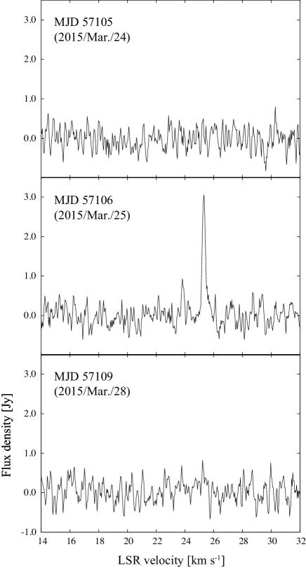
Figure 4: Typical flaring activity detected toward the spectral component G. Top, middle, and bottom panel shows the maser spectrum observed on MJD 57105, 57106, and 57109 (24, 25, and 28 March 2015), respectively.

3.2 Periodicity evaluated by Lomb-Scargle periodogram

We adopted the Lomb-Scargle (L-S) periodogram (Lomb (1976); Scargle (1982)) to evaluate periodicity for the flaring activities of the component G. This is the most reliable method to search for periodicity in flux variations of the methanol masers (Goedhart et al., 2014). In this paper, we regard an oversampling factor of 4 and frequencies with false-alarm probability $\leq 10^{-4}$ as significant, which are the same manner as Goedhart et al. (2014). The L-S periodogram adopted to all the data in MJD 56297–57408 is shown in figure 5, with the power level of 15.4 in the dashed line that corresponds to the false-alarm probability of $10^{-4}$. To avoid any bias, we used one 5-min scan for each day during the intraday monitoring, measured at the same azimuth and elevation angles as the other monitoring in section 2.1 and 2.2. We evaluated the period of 23.9 days as the significant detection (the power level of 39.2), corresponding to the frequency of $\sim$0.0419 cycle day^-1. We evaluated calculation errors to be $\pm 0.1$ days from the frequency resolution in the L-S periodogram.

The derived period of 23.9 days was also verified from comparison between observed flaring dates MJD_obs and expected ones from the periodicity. The expected flaring dates MJD_calc were calculated by $\mathrm{MJD}_{\mathrm{calc}}=\mathrm{MJD}_{0}+23.9\cdot n$ [day], where $n$ is an integer, and MJD${}_{0}=57275.4$ is the reference date estimated from the period II of the intraday monitoring. In the period II, it is difficult to define the accurate time when the component G reached its maximum on MJD 57275 (see figure 8b: relative MJD $=$ 2), causing errors of $\pm 0.5$ days at most in the flaring peak timing. The expected flaring dates for 47 flares are shown as solid and dashed lines in the lower panel of figure 3 and summarized in table 3.2. Until MJD 56745, spectra were obtained every 9–10 days, and thus no observations were executed within three days of MJD_calc for No. 2, 4, 8, 11–13, and 16. Also for the expected flares of No. 17–19 and 23, no observations were executed within three days of MJD_calc due to unavailability of the telescope. These are denoted by the symbol “$\cdots$” in column 3 of table 3.2. By excluding these expected flares, we compared 36 flares to evaluate whether the derived period is reasonable. As a result, 67% (24/36) of the observed flares coincide with the expected flaring dates within three days ($|\mathrm{MJD}_{\mathrm{obs}}-\mathrm{MJD}_{\mathrm{calc}}|\leq 1$ day: 14 flares, $1<|\mathrm{MJD}_{\mathrm{obs}}-\mathrm{MJD}_{\mathrm{calc}}|\leq 2$ days: 6 flares, and $2<|\mathrm{MJD}_{\mathrm{obs}}-\mathrm{MJD}_{\mathrm{calc}}|\leq 3$ days: 4 flares). On the other hand, no flares above 3.5$\sigma$ were detected at the dates out of three days of MJD_calc. The fact that the observed flares do not necessarily coincide with the expected flaring dates would not be attributed to the errors of 0.1 days in the L-S periodogram calculation and 0.5 days in the definition of the reference date MJD₀. No correlation was seen between $|\mathrm{MJD}_{\mathrm{obs}}-\mathrm{MJD}_{\mathrm{calc}}|$ and the periodic cycle $n$. The not necessarily coincidence can be attributed to the following two reasons: (1) Intrinsic difference in the time-scale of flux rising in the flaring activities may cause the difference of the observed flaring dates from the expected ones. Some flares might show the rising time over two days, one of which was observed in the period I of the intraday monitoring (see section 3.3). The peak timing of flares, therefore, might differ even in the case that the start timing of flares is same. (2) No observations in one day earlier or later than MJD_calc, occurred even in the observational dates during the daily monitoring from MJD 56784 (No. 25, 26, 28–35, 37, 38, and 47), may cause 1 day error in the difference between observed and expected flaring dates.

Non-detection might be attributed to an intrinsic property of the flaring component G. In the cases of $|\mathrm{MJD}_{\mathrm{obs}}-\mathrm{MJD}_{\mathrm{calc}}|\leq 1$ day, such as No. 7 and No. 14 in table 3.2, the non-detection is likely due to the absence of flare. The absence of flare is more strongly suggested in the period of more frequent observations (No. 20–47). The variability of flare amplitude might be due to a saturation level of the flaring maser gas. The time variation of the line width of the flaring component G implies an anti-correlation with the flux density as shown in figure 6. The line width in figure 6 is estimated as FWHM by the gaussian fitting, and the flare components brighter than the 5$\sigma$ detection of $\sim$1.5 Jy are plotted, which are well fitted within errors of 10%. According to model calculations, the line width tends to be narrower as its intensity increases, as long as the maser is unsaturated (Goldreich & Kwan, 1974). Under the condition of unsaturation, the logarithm of the flux density, $\log F$, is predicted to be proportional to the inverse square of the line width, $\Delta v^{-2}$. The best-fit result using $\log F=A+B\cdot\Delta v^{-2}$ is shown in figure 6, where the parameter $B$ is $0.033\pm 0.002$ while the parameter $A$ is fixed as the upper limit in a quiescent spectrum of 0.039 Jy (see section 3.4). Our results may suggest that the component G in the flaring phase is still unsaturated. The unsaturated state might cause the variability of flare amplitude and result in the non-detection of some flares, whose peak flux density should be lower than the detection limit. For instance, No. 20 flare having very weak peak flux density of 0.57 Jy observed in the period 0 of the intraday monitoring cannot be detected with the 3$\sigma$ detection limit of 0.9 Jy with the integration time of 5 min in the periodic monitoring (see section 3.3).

We conclude that the flaring activities of the spectral component G have regularly occurred with the period of 23.9$\pm 0.1$ days at least in 47 cycles, corresponding to $\sim$1,100 days. The derived period of 23.9 days is the shortest one observed in the masers at around high-mass YSOs so far, compared to 29.5 days in methanol (Goedhart et al., 2009), $\sim$2 yrs in silicon monoxide (Ukita et al., 1981), 237 days in formaldehyde (Araya et al., 2010), 25–30 days in hydroxyl (Green et al., 2012a), and 34.4 days in water (Szymczak et al., 2016).

Figure 5: L-S periodogram applied to the flaring spectral component G. A false-alarm probability $\leq 10^{-4}$, corresponding to the power level of 15.4, is denoted by a dashed horizontal line. The peak detected at the frequency around 0.084 cycle day^-1 with the power level of 26.3 must be a harmonic signal of the derived period as 23.9 days.

Figure 6: Relationship between the flux density and line width of the flaring component G. Filled squares represent the observed values showing flux densities brighter than the 5$\sigma$ detection of $\sim$1.5 Jy. A dashed line shows the best-fit result of the fitting; $\log F=A+B\cdot\Delta v^{-2}$, where the parameter $B$ is $0.033\pm 0.002$ while the parameter $A$ is fixed as the upper limit in a quiescent spectrum of 0.039 Jy (see section 3.4).

Comparison between observed and expected flaring dates for each flare in 47 periodic cycles. No. $n$ MJD_obs $F_{\mathrm{p}}$ MJD_calc Difference [day] [Jy] [day] [day] 1 $-$41 56297.0 3.5 56295.5 $+$1.5 2 $-$40 $\cdots$ 56319.4 3 $-$39 – $<0.70$ 56343.3 – 4 $-$38 $\cdots$ 56367.2 5 $-$37 – $<0.87$ 56391.1 – 6 $-$36 – $<0.85$ 56415.0 – 7 $-$35 – $<0.86$ 56438.9 – 8 $-$34 $\cdots$ 56462.8 9 $-$33 56486.5 2.3 56486.7 $-$0.2 10 $-$32 – $<0.90$ 56510.6 – 11 $-$31 $\cdots$ 56534.5 12 $-$30 $\cdots$ 56558.4 13 $-$29 $\cdots$ 56582.3 14 $-$28 – $<0.96$ 56606.2 – 15 $-$27 56633.1 1.2 56630.1 $+$3.0 16 $-$26 $\cdots$ 56654.0 17 $-$25 $\cdots$ 56677.9 18 $-$24 $\cdots$ 56701.8 19 $-$23 $\cdots$ 56725.7 20 $-$22 56749.8    0.57^∗ 56749.6 $+$0.2 21 $-$21 56773.8 2.1 56773.5 $+$0.3 22 $-$20 – $<0.90$ 56797.4 – 23 $-$19 $\cdots$ 56821.3 24 $-$18 56845.6 1.9 56845.2 $+$0.4 25 $-$17 56868.5 4.4 56869.1   $-$0.6^† 26 $-$16 56895.4 1.2 56893.0   $+$2.4^† 27 $-$15 56917.4 1.8 56916.9 $+$0.5 28 $-$14 56940.3 1.9 56940.8   $-$0.5^† 29 $-$13 56963.2 1.3 56964.7   $-$1.5^† 30 $-$12 56990.2 1.2 56988.6   $+$1.6^† 31 $-$11 57012.1 2.1 57012.5   $-$0.4^† 32 $-$10 – $<0.91$ 57036.4   –^† 33 $-$9 57058.0 3.2 57060.3   $-$2.3^† 34 $-$8 57082.9 6.6 57084.2   $-$1.3^† 35 $-$7 57106.8 3.1 57108.1   $-$1.3^† 36 $-$6 57130.8 1.3 57132.0 $-$1.2 37 $-$5 – $<0.90$ 57155.9   –^† 38 $-$4 – $<0.82$ 57179.8   –^† 39 $-$3 – $<0.91$ 57203.7 – 40 $-$2 57227.5 6.5 57227.6 $-$0.1 41 $-$1 57251.4 4.3 57251.5 $-$0.1 42^‡ 0 57275.4 4.2 57275.4    0.0 43 $+$1 57298.3 3.5 57299.3 $-$1.0 44 $+$2 57323.2 6.7 57323.2    0.0 45 $+$3 57347.2 6.3 57347.1 $+$0.1 46 $+$4 57373.1 5.5 57371.0 $+$2.1 47 $+$5 – $<0.76$ 57394.9   –^† Column 1: Identification number of each flare; Column 2: Periodic cycle of each flare from the reference flare No. 42 (the integer used in section 3.2); Columns 3, 4: Observed flaring date and flux density. “$\cdots$” denotes that no observations were executed within three days of the expected flaring date, while “–” shows no detection of the flares.; Column 5: Expected flaring date; Column 6: Difference between observed and expected flaring dates.
Note. – ^∗Detected thanks to high-sensitivity as the detection limit 3$\sigma$ of 0.19 Jy achieved by the integration of all the data in MJD 56750 (see section 3.3); ^†there are no observations in one day earlier or later than MJD_calc during the daily monitoring from MJD 56784 (see section 3.2); ^‡reference date for the calculation of the expected flaring dates.

3.3 Flux variability in the intraday monitoring

We present flux variability obtained through the intraday monitoring described in section 2.3. In the period 0, the flaring activities were detected twice in the component G, as shown in figure 7. Each point shows the data obtained by the integration of all the data in each observational date. The integration time is $\sim$1.8 hrs (110 min) and $\sim$3.3 hrs (195 min) in MJD 56745–56774 and 56775–56778, respectively, yielding typical detection limits (3$\sigma$) of 0.15–0.20 Jy. The first flare occurred on MJD 56750 and 56751. On MJD 56750, the flux density was reached to the maximum of 0.57 Jy with the signal to noise ratio of $\sim$9. It was not detected in the periodic monitoring with the integration time of 5 min that yielded the detection limit (3$\sigma$) of $\sim$0.9 Jy. This flaring component decayed to 0.25 Jy, which was close to the detection limit, on MJD 56751, and disappeared on the next day (MJD 56752). The second flare occurred on MJD 56774–56777. The peak flux density was 2.2 Jy, and an e-folding time for decay was estimated to be 1.3 days.

Figure 8(a)–(d) show results obtained in the periods I–IV of the intraday monitoring, respectively. The flare of the component G was detected in all the periods. In the period I, the rising time to the peak flux density of $\sim$5 Jy was two days, and almost same days were spent for decaying, showing a symmetric profile of flux variability. On the other hand, asymmetric profiles were obtained in the periods II and IV. In the periods II and IV, the peak flux densities were $\sim$4.5 and 7.0 Jy. The rising time was two days, while the decay has the e-folding time of 2.7 and 2.6 days, respectively. In the period III, no decay part of flux variability was observed. The rising time to the peak flux density of $\sim$3.5 Jy was within one day, while the decaying time seems to be longer judging from figure 8(c), being suggestive of an asymmetric profile.

Interestingly, we detected the rising time accurately in the period III. No emission was detected from an integrated spectrum on MJD 57296 (relative MJD $=$ 0 in figure 8c) and from the first scan at 4:45:55 UT to the scan at 6:29:35 UT on MJD 57297. At the next scan at 7:09:00 UT on MJD 57297, the flaring component G was detected for the first time in this period above 3$\sigma$ of 0.9 Jy with 5 min integration, and then it rose up. Although a turning point from rising to decaying was not detected on the next day (MJD 57298) since the maximum flux density in this period occurred on the first scan 4:27:00 UT, the rising time was stringently evaluated to be $\leq$ 21.3 hrs (1,278 min). This is regarded as an upper limit of the rising time of the flare.

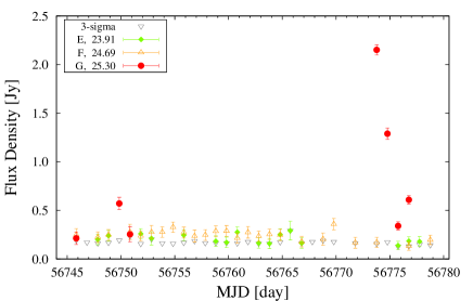
Figure 7: Flux variation detected in the period 0 of the intraday monitoring. Each point shows the data obtained by the integration of all the data in each observational date. Each symbol showing each spectral component is unified with one used in figure 3. The error bar represents the standard deviation in each date.

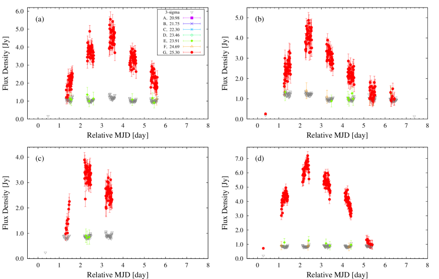
Figure 8: Same as figure 7 but for the periods I–IV shown in panels (a)–(d), respectively. The horizontal axis is MJD relative to the reference date of 57248, 57273, 57296, and 57321 in each panel, respectively. The reference date is defined as the previous day from the date when the flaring component is detected in one 5-min scan for the first time in each period. In the case of no detection in all 5-min scans through each observational date, an integration with all the data in each date was performed to obtain better sensitivities, yielding the detection limit (3$\sigma$) of $\sim$0.15–0.20 Jy.

3.4 Typical spectrum in a quiescent phase

In this section, we evaluate a ratio of the peak flux density in the flaring and quiescent (non-flaring) phases. The quiescent phase MJD_q is defined by $\mathrm{MJD}_{\mathrm{q}}=\bigl{(}\mathrm{MJD}_{0}+23.9\cdot\left(n-0.5\right)\bigr{)}\pm 5$ [days], where $n$ is an integer, and MJD₀ 57275.4 is the reference date (see section 3.2). We also picked up data taken from the intraday periods 0–IV, even in the case of being observed at different azimuth and elevation angles to obtain the best detection limit.

As a result, a spectrum in the quiescent phase was obtained from 561 scans of 5 min duration, or $\sim$46.8 hrs (2,805 min) integration time in total (figure 9), under an assumption that the emission in quiescent intervals was stable. A detection limit (3$\sigma$) was achieved to be 0.039 Jy. Five components whose flux densities were 0.15–0.3 Jy were detected in the $V_{\mathrm{lsr}}$ of 22–25 km s^-1, roughly supposed as the components C–F. On the other hand, no emission was detected at the $V_{\mathrm{lsr}}=$ 25.30 km s^-1 of the flaring component G (dashed line in figure 9). We concluded that the ratio of the peak flux density in the flaring and quiescent phases was more than 180 when the flare showed the maximum peak flux density of $\sim$7 Jy.

Figure 9: Spectrum in the quiescent phase defined in section 3.4. All the selected 561 scans of 5 min duration were used. The 3$\sigma$ detection limit was achieved to be 0.039 Jy. A dashed vertical line denotes the LSR velocity of the flaring component G (25.30 km s^-1).

3.5 Comparison with other flaring sources

We compare the flaring activities detected in the 6.7 GHz methanol maser of G 014.23 to flares observed in other 6.7 GHz maser sources. First, in the point of view of the ratio of the peak flux density in the flare and quiescence, the flares at the component G in G 014.23 can be compared to a spectral component of $V_{\mathrm{lsr}}=$ $-$5.88 km s^-1 in G 351.42$+$00.64 (NGC6334 F: Goedhart et al. (2004)) and those of $V_{\mathrm{lsr}}=$ $-$1.32 and $-$0.55 km s^-1 in Cepheus A (Szymczak et al., 2014). The spectral components in both sources showed ratios of the peak flux density in the flare of 170 and 240 in comparison with the quiescent phase. It is also similar that only a part of spectral components show remarkable flux variability. The time scale of the flux rising, however, is different, i.e., approximately two and one months in G 351.42$+$00.64 and Cepheus A respectively, while two days or less in G 014.23. Second, in the point of view of the time scale of the flux rising, the flares in G 014.23 can be compared to flaring activities of a spectral component of $V_{\mathrm{lsr}}=$ 59.6 km s^-1 in G 033.64$-$00.22 that showed the time scale of the flux rising of one day or less (Fujisawa et al. (2012), fujisawa14b). Ratios of the peak flux density in the flares of G 033.64$-$00.22 were, however, $\sim$7–27 in comparison with the quiescent phase and approximately one order of magnitude less than that in G 014.23. Finally, in the point of view of periodicity, the periodic flares in G 014.23 can be compared to periodic flaring activities detected in IRAS 22198$+$6336 that showed the period of 34.6 days (Fujisawa et al., 2014a). Both the time scale of flux rising is comparable as short as two to three days or less. A ratio of the peak flux density in the flare of IRAS 22198$+$6336 was, however, more than 30 in comparison with the quiescent phase, i.e., one-fifth of the case in G 014.23, though it might be affected by poor detection limits (3$\sigma$) of $\sim$1.3 Jy in observations for IRAS 22198$+$6336. Furthermore, periodic flares occurred on all the spectral components with the time lag of two days in IRAS 22198$+$6336, while on only the single spectral component G in G 014.23.

We concluded that the flaring activities detected in G 014.23 are remarkable phenomena because of the large ratio of the peak flux density in comparison with the quiescent phase, the short time scale of the flux rising, the occurrence on just one spectral component, and the short periodicity.

4 Discussions

We discuss possible mechanisms to explain the intermittent periodic flares in the component G of G 014.23, including their ratio of the peak flux density more than 180 in the flaring and quiescent phases, the time scale of the flux rising as short as two days, either the symmetric or asymmetric profile in each flare, and the period of 23.9 days.

It was reported that interstellar scintillation caused flux variability on the time scale as short as minutes observed in hydroxyl masers (Clegg & Cordes, 1991). This model, however, explains amplitude fluctuations with at most 20% and is not suited to the flares in G 014.23. Furthermore, if the scintillation causes the flares, all the spectral components would show flux variability with the same pattern. Therefore, the flares were not caused by interstellar scintillation.

The amplifying effect by overlapping two maser clouds along the line of sight (Deguchi & Watson, 1989) could cause flaring activities and explain distinct ratio of flux densities with one magnitude or more brighter in comparison with quiescent phases. This effect was verified toward the outburst of the 22.2 GHz water maser in Orion KL (Shimoikura et al., 2005). The period of 23.9 days, however, is too short unless the maser emission would directly originate from the circumstellar disk in Keplerian rotation. Assuming that the central mass is 3.3 (Povich & Whitney, 2010) and 8 (typical one and the lower limit as a high-mass star), the period of 23.9 days is achieved at the radius of 0.2 and 0.3 au in the Keplerian disk, respectively. At these radii, the dust temperature $T_{\mathrm{dust}}$ should be higher than 1,000 K that is out of range for the 6.7 GHz methanol maser excitation 100 K $\leq T_{\mathrm{dust}}\leq 300$ K (Cragg et al., 2005). Therefore, the overlapping model was not applicable to the periodic flares in G 014.23 with the period of 23.9 days.

The magnetic reconnection around a central star can release the energy to heat the gas and dust localized at a flaring area and explain flaring activities with rising time scale of a few days or less, such as ones in G 033.64$-$00.22 (Fujisawa et al. (2012), fujisawa14b). The periodic flux variations persisting at least in 47 cycles as shown in the lower-panel of figure 3 and table 3.2, however, can be hardly explained by the magnetic reconnection.

The stellar pulsation of a high-mass YSO can produce the periodic flux variability through the change of dust temperature in the maser clouds (Inayoshi et al., 2013). All the spectral components should be affected in this pulsation model. The model of combining a constant and an independent pulsating YSOs is suggested to explain a periodic flux variation occurred in part of the components (Sanna et al., 2015). However, it is difficult to produce the intermittent pattern because the pulsation is driven by the $\kappa$ mechanism (van der Walt et al., 2016). Therefore, the periodic flares in G 014.23 that occurred only on one component G showing the intermittent pattern cannot be explained by the pulsation model.

The circumbinary disk model is also proposed to explain the periodic variability in some methanol sources through variations of the dust temperature (Araya et al., 2010). However, this model is not suited to the periodic flares in G 014.23 since it is difficult to cause periodic variations toward only one in seven spectral components as in the case of the pulsation model.

The CWB model can produce the intermittent flux variability through the periodic change of the seed photon flux caused by periodically forming shocks at periastron due to collision of stellar winds (van der Walt et al. (2009); van der Walt (2011)). The ionizing radiation that originates from the shocks propagates through an HII region and changes the electron density resulting in periodic variability of the free-free emission. There has been a non-detection of an HII region in G 014.23 with typical rms noise level of $\sim$0.3 mJy beam^-1 from the unbiased catalog for HII regions made through the CORNISH survey project (Co-ordinated Radio and Infrared Survey for High Mass Star Formation: Hoare et al. (2012); Purcell et al. (2013)). The high-sensitivity survey (rms levels of $\sim$3–10 $\mu$Jy beam^-1) using the Karl G. Jansky Very Large Array (JVLA), however, detected weak and compact radio continuum emissions toward 58 high-mass star forming regions, most of which were non-detections in the CORNISH (Rosero et al., 2016). Although the YSO associated with G 014.23 whose evolutionary phase is classified into the stage 0/I may be too early to form HII regions, we need to conduct a high-sensitivity observation using the JVLA for verification whether an HII region exists in G 014.23.

The dust temperature variation of the accretion disk around a protobinary caused by periodic rotation of hot and dense spiral shock wave in the disk central gap (Parfenov & Sobolev, 2014) might be another candidate for explanation of the periodic flares in G 014.23, although some properties of this model might be improved in the suggestion by van der Walt et al. (2016). This model can cause a flare toward only maser components localized along the line of sight between the central YSO and the maser-emitting region, which are illuminated by the hot component associated with the spiral shock as an extra heating source. The extra heat results in increment of column densities suitable for the maser excitation and amplifying a maser. The spiral shock is periodically rotated by the binary system and thus can cause periodic flares of the maser. It was noted by van der Walt et al. (2016) that the spiral shock model could not account for the intermittent pattern in periodic variations due to a tail of the shock. This issue could be resolved by replacing the extra heating source of the spiral shock with a shock formed by the CWB system within the disk central gap. Another issue noted by van der Walt et al. (2016) was that the luminosity of the spiral shock might be too low to play a role as the extra heating source. This issue was predicted from densities of gases in the gap region and of postshocked gases in the spiral shock at least five orders of magnitude lower than that used in the spiral shock model, which were estimated from a hydrogen density at the inner edge of the circumbinary disk assumed by Parfenov & Sobolev (2014). The same issue occurs even in the case of an improved model by replacing with the shock by the CWB (van der Walt et al., 2016). The issue of the low luminosity is unresolved, but this may be overcome under the unsaturated state (see section 3.2 and figure 6), causing strong flux variability by a bit of increment of column densities expected from the exponential relationship with the path length of the masing gas.

To evaluate applicability of the shock model by the CWB within the disk central gap, we estimated the orbital semi-major axis of the binary to be 0.26 and 0.34 au from the period of 23.9 days in the case of the mass of a central primary YSO 3.3 and typical high-mass star of 8 with the companion mass of 1 , respectively. The orbital semi-major axis never interferes with the primary star having the radius of 0.07 and 0.08 au estimated in the case of the mass of 3.3 and 8 , respectively, under the condition of the mass accretion rate 10^-4  yr^-1 (see equation (13) of Hosokawa & Omukai (2009)). In the point of view of time scale of the flux rising, the dust in the maser emitting region in the disk is heated mostly by a diffuse emission from the ionized gas within the inner disk regions that in turn is re-processed stellar and shocked gas radiation. The diffuse emission produces the heating rate of order of 10^-13 erg s^-1 cm^-3, resulting in the time scale of the order of a few hours for increasing $T_{\mathrm{dust}}$ by 10 K (Parfenov & Sobolev, 2014). The time scale for increasing $T_{\mathrm{dust}}$ by 100 K, therefore, is expected to be a few tens of hours, which is comparable to the time scale of the flux rising for the flaring component G, i.e., 21.3 hrs (1,278 min). While the profile of the flare in the period I of the intraday monitoring is symmetric with respect to its peak, those in the periods II and IV (and possibly in the period III) are asymmetric. These differences might be attributed to an inclination angle of the binary suggested in three-dimensional numerical models (Sytov et al., 2009). In the numerical model, the variation profile of the column density depends on the inclination angle of the binary, possibly shaping the profile of flares. Both symmetric and asymmetric profiles might happen if the inclination of the binary is close to the critical value for the inclination. To verify the inclination angle, we plan to obtain a spatial distribution of the maser emissions in G 014.23 through a very-long-baseline-interferometry (VLBI) observation. For instance, if we obtain elliptical morphology, the inclination angle can be estimated under an assumption that all the masers are distributed on a concentric circle in a disk.

We conclude that the models of the change in the flux of seed photons by the CWB system or the variation of the dust temperature by the CWB shock within the disk central gap, in which the orbital semi-major axes of the binary are 0.26–0.34 au, might explain all the characteristics of the intermittent periodic flare of the component G in G 014.23: the ratio of the peak flux density in the flare was more than 180 in comparison with the quiescent phase, the time scale of the flux rising was as short as two days or less, the flare was decayed with either the symmetric or asymmetric profile in each flare, and the period was short as 23.9 days.

5 Summary

We presented periodic and flaring flux variability of the 6.7 GHz methanol maser emission detected in the spectral component G ($V_{\mathrm{lsr}}=$ 25.30 km s^-1) in G 014.23$-$00.50 through a long-term and highly frequent monitoring using the Hitachi 32-m radio telescope. The flaring activities have regularly occurred with the period of 23.9$\pm 0.1$ days at least in 47 cycles from 5 January 2013 to 21 January 2016 (MJD 56297–57408), corresponding to $\sim$1,100 days. The period of 23.9 days is the shortest one observed in the masers at around high-mass YSOs so far. The flaring component normally fell below the detection limit (3$\sigma$) of $\sim$0.9 Jy. In the flaring periods, the component rose above the detection limit with the ratio of the peak flux density more than 180 in comparison with the quiescent phase, showing the intermittent periodic variability. The time-scale of the flux rising was typically two days or shorter, and the flaring components were decayed with either symmetric or asymmetric profile, which were revealed through the intraday monitoring. These characteristics might be explained in the models of the change in the flux of seed photons by the CWB system or the variation of the dust temperature by the CWB shock within the disk central gap, in which the orbital semi-major axes of the binary were estimated to be 0.26–0.34 au.

The authors are grateful to Naoko Furukawa for substantial contributions to this monitoring project. Thanks are due to all the staff and students both at Ibaraki University and those graduated from the university, and the staff of the Mizusawa VLBI observatory and the members of the Japanese VLBI Network team, for the development and operation of the Hitachi 32-m radio telescope. The authors would also like to thank the anonymous referee for useful and constructive suggestions to improve the paper and Dr. Gemma Busquet for kindly sharing their calibrated SMA data in the fits format with us. This work was financially supported in part by a Grant-in-Aid for Scientific Research (KAKENHI) from Japan Society for the Promotion of Science (JSPS), No. 24340034.

References

- Araya et al. (2010) Araya, E. D., Hofner, P., Goss, W. M., Kurtz, S., Richards, A. M. S., Linz, H., Olmi, L., & Sewiło, M. 2010, ApJ, 717, L133
- Breen et al. (2015) Breen, S. L., et al. 2015, MNRAS, 450, 4109
- Busquet et al. (2013) Busquet, G., et al. 2013, ApJ, 764, L26
- Busquet et al. (2016) Busquet, G., et al. 2016, ApJ, 819, 139
- Caswell et al. (2010) Caswell, J. L., et al. 2010, MNRAS, 404, 1029
- Caswell et al. (2011) Caswell, J. L., et al. 2011, MNRAS, 417, 1964
- Clegg & Cordes (1991) Clegg, A. W., & Cordes, J. M. 1991, ApJ, 374, 150
- Cragg et al. (2005) Cragg, D. M., Sobolev, A. M., & Godfrey, P. D. 2005, MNRAS, 360, 533
- Cyganowski et al. (2008) Cyganowski, C. J., et al. 2008, AJ, 136, 2391-2412
- Deguchi & Watson (1989) Deguchi, S., & Watson, W. D. 1989, ApJ, 340, L17
- Elmegreen and Lada (1976) Elmegreen, B. G., & Lada, C. J. 1976, AJ, 81, 1089
- Fujisawa et al. (2012) Fujisawa, K., et al. 2012, PASJ, 64,
- Fujisawa et al. (2014a) Fujisawa, K., et al. 2014a, PASJ, 66, 78
- Fujisawa et al. (2014b) Fujisawa, K., et al. 2014b, PASJ, 66, 109
- Goedhart et al. (2003) Goedhart, S., Gaylard, M. J., & van der Walt, D. J. 2003, MNRAS, 339, L33
- Goedhart et al. (2004) Goedhart, S., Gaylard, M. J., & van der Walt, D. J. 2004, MNRAS, 355, 553
- Goedhart et al. (2009) Goedhart, S., Langa, M. C., Gaylard, M. J., & van der Walt, D. J. 2009, MNRAS, 398, 995
- Goedhart et al. (2014) Goedhart, S., Maswanganye, J. P., Gaylard, M. J., & van der Walt, D. J. 2014, MNRAS, 437, 1808
- Goldreich & Kwan (1974) Goldreich, P., & Kwan, J. 1974, ApJ, 190, 27
- Green et al. (2010) Green, J. A., et al. 2010, MNRAS, 409, 913
- Green et al. (2012a) Green, J. A., Caswell, J. L., Voronkov, M. A., & McClure-Griffiths, N. M. 2012a, MNRAS, 425, 1504
- Green et al. (2012b) Green, J. A., et al. 2012b, MNRAS, 420, 3108
- Hoare et al. (2012) Hoare, M. G., et al. 2012, PASP, 124, 939
- Hosokawa & Omukai (2009) Hosokawa, T., & Omukai, K. 2009, ApJ, 691, 823
- Inayoshi et al. (2013) Inayoshi, K., Sugiyama, K., Hosokawa, T., Motogi, K., & Tanaka, K. E. I. 2013, ApJ, 769, L20
- Kondo et al. (2008) Kondo, T., Koyama, Y., Ichikawa, R., Sekido, M., Kawai, E. & Kimura, M. 2008, J. Geod. Soc. Jpn, 54, 233
- Lomb (1976) Lomb, N. R. 1976, Ap&SS, 39, 447
- Maswanganye et al. (2015) Maswanganye, J. P., Gaylard, M. J., Goedhart, S., Walt, D. J. v. d., & Booth, R. S. 2015, MNRAS, 446, 2730
- Maswanganye et al. (2016) Maswanganye, J. P., van der Walt, D. J., Goedhart, S., & Gaylard, M. J. 2016, MNRAS, 456, 4335
- Ohashi et al. (2016) Ohashi, S., Sanhueza, P., Chen, H.-R. V., Zhang, Q., Busquet, G., Nakamura, F., Palau, A., & Tatematsu, K. 2016, ApJ, 833, 209
- Okoh et al. (2014) Okoh, D., Esimbek, J., Zhou, J. J., Tang, X. D., Chukwude, A., Urama, J., & Okeke, P. 2014, Ap&SS, 350, 657
- Olmi et al. (2014) Olmi, L., Araya, E. D., Hofner, P., Molinari, S., Morales Ortiz, J., Moscadelli, L., & Pestalozzi, M. 2014, A&A, 566, A18
- Parfenov & Sobolev (2014) Parfenov, S. Y., & Sobolev, A. M. 2014, MNRAS, 444, 620
- Peretto and Fuller (2009) Peretto, N., & Fuller, G. A. 2009, A&A, 505, 405
- Pestalozzi et al. (2005) Pestalozzi, M. R., Minier, V., & Booth, R. S. 2005, A&A, 432, 737
- Povich & Whitney (2010) Povich, M. S., & Whitney, B. A. 2010, ApJ, 714, L285
- Purcell et al. (2013) Purcell, C. R., et al. 2013, ApJS, 205, 1
- Robitaille et al. (2006) Robitaille, T. P., Whitney, B. A., Indebetouw, R., Wood, K., & Denzmore, P. 2006, ApJS, 167, 256
- Rosero et al. (2016) Rosero, V., Hofner, P., Claussen, M., et al. 2016, ApJS, 227, 25
- Sanna et al. (2015) Sanna, A., et al. 2015, ApJ, 804, L2
- Scargle (1982) Scargle, J. D. 1982, ApJ, 263, 835
- Schlingman et al. (2011) Schlingman, W. M., et al. 2011, ApJS, 195, 14
- Sewilo et al. (2004) Sewilo, M., Watson, C., Araya, E., Churchwell, E., Hofner, P., & Kurtz, S. 2004, ApJS, 154, 553
- Shimoikura et al. (2005) Shimoikura, T., Kobayashi, H., Omodaka, T., Diamond, P. J., Matveyenko, L. I., & Fujisawa, K. 2005, ApJ, 634, 459
- Shirley et al. (2013) Shirley, Y. L., et al. 2013, ApJS, 209, 2
- Sun et al. (2014) Sun, Y., et al. 2014, A&A, 563, A130
- Sytov et al. (2009) Sytov, A. Y., Bisikalo, D. V., Kaigorodov, P. V., & Boyarchuk, A. A. 2009, Astronomy Reports, 53, 428
- Szymczak et al. (2011) Szymczak, M., Wolak, P., Bartkiewicz, A., & van Langevelde, H. J. 2011, A&A, 531, L3
- Szymczak et al. (2014) Szymczak, M., Wolak, P., & Bartkiewicz, A. 2014, MNRAS, 439, 407
- Szymczak, Wolak, and Bartkiewicz (2015) Szymczak, M., Wolak, P., & Bartkiewicz, A. 2015, MNRAS, 448, 2284
- Szymczak et al. (2016) Szymczak, M., Olech, M., Wolak, P., Bartkiewicz, A., & Gawroński, M. 2016, MNRAS, 459, L56
- Ukita et al. (1981) Ukita, N., Kaifu, N., Chikada, Y., Miyaji, T., & Miyazawa, K. 1981, PASJ, 33, 341
- van der Walt et al. (2009) van der Walt, D. J., Goedhart, S., & Gaylard, M. J. 2009, MNRAS, 398, 961
- van der Walt (2011) van der Walt, D. J. 2011, AJ, 141, 152
- van der Walt et al. (2016) van der Walt, D. J., Maswanganye, J. P., Etoka, S., Goedhart, S., & van den Heever, S. P. 2016, A&A, 588, A47
- Wang et al. (2006) Wang, Y., Zhang, Q., Rathborne, J. M., Jackson, J., & Wu, Y. 2006, ApJ, 651, L125
- Xu et al. (2009) Xu, Y., Voronkov, M. A., Pandian, J. D., Li, J. J., Sobolev, A. M., Brunthaler, A., Ritter, B., & Menten, K. M. 2009, A&A, 507, 1117
- Xu et al. (2011) Xu, Y., Moscadelli, L., Reid, M. J., Menten, K. M., Zhang, B., Zheng, X. W., & Brunthaler, A. 2011, ApJ, 733, 25
- Yonekura et al. (2016) Yonekura, Y., et al. 2016, PASJ, 68, 74