Group Importance Sampling for Particle Filtering and MCMC

Abstract

Bayesian methods and their implementations by means of sophisticated Monte Carlo techniques have become very popular in signal processing over the last years. Importance Sampling (IS) is a well-known Monte Carlo technique that approximates integrals involving a posterior distribution by means of weighted samples. In this work, we study the assignation of a single weighted sample which compresses the information contained in a population of weighted samples. Part of the theory that we present as Group Importance Sampling (GIS) has been employed implicitly in different works in the literature. The provided analysis yields several theoretical and practical consequences. For instance, we discuss the application of GIS into the Sequential Importance Resampling framework and show that Independent Multiple Try Metropolis schemes can be interpreted as a standard Metropolis-Hastings algorithm, following the GIS approach. We also introduce two novel Markov Chain Monte Carlo (MCMC) techniques based on GIS. The first one, named Group Metropolis Sampling method, produces a Markov chain of sets of weighted samples. All these sets are then employed for obtaining a unique global estimator. The second one is the Distributed Particle Metropolis-Hastings technique, where different parallel particle filters are jointly used to drive an MCMC algorithm. Different resampled trajectories are compared and then tested with a proper acceptance probability. The novel schemes are tested in different numerical experiments such as learning the hyperparameters of Gaussian Processes, two localization problems in a wireless sensor network (with synthetic and real data) and the tracking of vegetation parameters given satellite observations, where they are compared with several benchmark Monte Carlo techniques. Three illustrative Matlab demos are also provided.

Keywords: Importance Sampling, Markov Chain Monte Carlo (MCMC), Particle Filtering, Particle Metropolis-Hastings, Multiple Try Metropolis, Bayesian Inference

1 Introduction

Bayesian signal processing, which has become very popular over the last years in statistical signal processing, requires the study of complicated distributions of variables of interested conditioned on observed data (Liu, 2004; Martino and Míguez, 2009; Martino et al., 2014a; Robert and Casella, 2004). Unfortunately, the computation of statistical features related to these posterior distributions (such as moments or credible intervals) is analytically impossible in many real-world applications. Monte Carlo methods are state-of-the-art tools for approximating complicated integrals involving sophisticated multidimensional densities (Liang et al., 2010; Liu, 2004; Robert and Casella, 2004). The most popular classes of MC methods are the Importance Sampling (IS) techniques and the Markov chain Monte Carlo (MCMC) algorithms (Liang et al., 2010; Robert and Casella, 2004). IS schemes produce a random discrete approximation of the posterior distribution by a population of weighted samples (Bugallo et al., 2015; Martino et al., 2017a, 2015; Liu, 2004; Robert and Casella, 2004). MCMC techniques generate a Markov chain (i.e., a sequence of correlated samples) with a pre-established target probability density function (pdf) as invariant density (Liang et al., 2010; Liu, 2004). Both families are widely used in the signal processing community. Several exhaustive overviews regarding the application of Monte Carlo methods in statistical signal processing, communications and machine learning can be found in the literature: some of them specifically focused on MCMC algorithms (Andrieu et al., 2003; Dangl et al., 2006; Fitzgerald, 2001; Martino, 2018), others specifically focused on IS techniques (and related methods) (Bugallo et al., 2017, 2015; Djurić et al., 2003; Elvira et al., 2015a) or with a broader view (Candy, 2009; Wang et al., 2002; Doucet and Wang, 2005; Pereyra et al., 2016; Ruanaidh and Fitzgerald, 2012).

In this work, we introduce theory and practice of a novel approach, called Group Importance Sampling (GIS), where the information contained in different sets of weighted samples is compressed by using only one, yet properly selected, particle, and one suitable weight. This general idea supports the validity of different Monte Carlo algorithms in the literature: interacting parallel particle filters (Bolić et al., 2005; Míguez and Vázquez, 2016; Read et al., 2014), particle island schemes and related techniques (Verg et al., 2015, 2014; Whiteley et al., 2016), particle filters for model selection (Drovandi et al., 2014; Martino et al., 2017c; Urteaga et al., 2016), nested Sequential Monte Carlo (SMC) methods (Naesseth et al., 2015, 2016; Stern, 2015) are some examples. We point out some consequences of the application of GIS in Sequential Importance Resampling (SIR) schemes, allowing partial resampling procedures and the use of different marginal likelihood estimators. Then, we show that the Independent Multiple Try Metropolis (I-MTM) techniques and the Particle Metropolis-Hastings (PMH) algorithm can be interpreted as a classical Independent Metropolis-Hastings method by the application of GIS.

Furthermore, we present two novel techniques based on GIS. The first one is the Group Metropolis Sampling (GMS) algorithm that generates a Markov chain of sets of weighted samples. All these resulting sets of samples are jointly exploited to obtain a unique particle approximation of the target distribution. On the one hand, GMS can be considered an MCMC method since it produces a Markov chain of sets of samples. On the other hand, the GMS can be also considered as an iterated importance sampler where different estimators are finally combined in order to build a unique IS estimator. This combination is obtained dynamically through random repetitions given by MCMC-type acceptance tests. GMS is closely related to Multiple Try Metropolis (MTM) techniques and Particle Metropolis-Hastings (PMH) algorithms (Andrieu et al., 2010; Bédard et al., 2012; Casarin et al., 2013; Craiu and Lemieux, 2007; Martino and Read, 2013; Martino and Louzada, 2017), as we discuss below. The GMS algorithm can be also seen as an extension of the method in (Casella and Robert, 1996), for recycling auxiliary samples in a MCMC method.

The second novel algorithm based on GIS is the Distributed PMH (DPMH) technique where the outputs of several parallel particle filters are compared by an MH-type acceptance function. The proper design of DPMH is a direct application of GIS. The benefit of DPMH is twofold: different type of particle filters (for instance, with different proposal densities) can be jointly employed, and the computational effort can be distributed in several machines speeding up the resulting algorithm. As the standard PMH method, DPMH is useful for filtering and smoothing the estimation of the trajectory of a variable of interest in a state-space model. Furthermore, the marginal version of DPMH can be used for the joint estimation of dynamic and static parameters. When the approximation of only one specific moment of the posterior is required, like GMS, the DPMH output can be expressed as a chain of IS estimators. The novel schemes are tested in different numerical experiments: hyperparameter tuning for Gaussian Processes, two localization problems in a wireless sensor network (one with real data), and finally a filtering problem of Leaf Area Index (LAI), which is a parameter widely used to monitor vegetation from satellite observations. The comparisons with other benchmark Monte Carlo methods show the benefits of the proposed algorithms.

The remainder of the paper has the following structure. Section 2 recalls some background material. The basis of the GIS theory is introduced in Section 3. The applications of GIS in particle filtering and Multiple Try Metropolis algorithms are discussed in Section 4. In Section 5, we introduce the novel techniques based on GIS. Section 6.1 provides the numerical results and in Section 7 we discuss some conclusions.

2 Problem statement and background

In many applications, the goal is to infer a variable of interest, ${\bf x}=x_{1:D}=[x_{1},x_{2},\ldots,x_{D}]\in\mathcal{X}\subseteq\mathbb{R}^{D\times\xi}$, where $x_{d}\in\mathbb{R}^{\xi}$ for all $d=1,\ldots,D$, given a set of related observations or measurements, ${\bf y}\in\mathbb{R}^{d_{Y}}$. In the Bayesian framework all the statistical information is summarized by the posterior probability density function (pdf), i.e.,

$$\bar{\pi}({\bf x})=p({\bf x}|{\bf y})=\frac{\ell({\bf y}|{\bf x})g({\bf x})}{Z({\bf y})},$$ (1)

where $\ell({\bf y}|{\bf x})$ is the likelihood function, $g({\bf x})$ is the prior pdf and $Z({\bf y})$ is the marginal likelihood (a.k.a., Bayesian evidence). In general, $Z\equiv Z({\bf y})$ is unknown and difficult to estimate in general, so we assume to be able to evaluate the unnormalized target function,

$$\pi({\bf x})=\ell({\bf y}|{\bf x})g({\bf x}).$$ (2)

The computation of integrals involving $\bar{\pi}({\bf x})=\frac{1}{Z}\pi({\bf x})$ is often intractable. We consider the Monte Carlo approximation of complicated integrals involving the target $\bar{\pi}({\bf x})$ and an integrable function $h({\bf x})$ with respect to $\bar{\pi}$, i.e.,

$$I=E_{\bar{\pi}}[h({\bf X})]=\int_{\mathcal{X}}h({\bf x})\bar{\pi}({\bf x})d{\bf x},$$ (3)

where we denote ${\bf X}\sim\bar{\pi}({\bf x})$. The basic Monte Carlo (MC) procedure consists in drawing $N$ independent samples from the target pdf, i.e., ${\bf x}_{1},\ldots,{\bf x}_{N}\sim\bar{\pi}({\bf x})$, so that ${\widehat{I}}_{N}=\frac{1}{N}\sum_{n=1}^{N}h({\bf x}_{n})$ is an unbiased estimator of $I$ (Liu, 2004; Robert and Casella, 2004). However, in general, direct methods for drawing samples from $\bar{\pi}({\bf x})$ do not exist so that alternative procedures are required. Below, we describe the most popular approaches. Table 1 summarizes the main notation of the work. Note that the words sample and particle are used as synonyms along this work. Moreover, Table 2 shows the main used acronyms.

Marginal Likelihood.

As shown above, we consider a target function $\bar{\pi}({\bf x})=\frac{1}{Z}\pi({\bf x})$ that is posterior density, i.e., $\bar{\pi}({\bf x})=p({\bf x}|{\bf y})=\frac{\ell({\bf y}|{\bf x})g({\bf x})}{Z({\bf y})}$ and $\pi({\bf x})=\ell({\bf y}|{\bf x})g({\bf x})$. In this case, $Z=Z({\bf y})=\int_{\mathcal{X}}\ell({\bf y}|{\bf x})g({\bf x})d{\bf x}$ represents the marginal probability of ${\bf y}$, i.e., $Z({\bf y})=p({\bf y})$ that is usually called marginal likelihood (or Bayesian evidence). This quantity is important for model selection purpose. More generally, the considerations in the rest of the work are valid also for generic target densities $\bar{\pi}({\bf x})=\frac{1}{Z}\pi({\bf x})$ where $\pi({\bf x})\geq 0$ and $Z=\int_{\mathcal{X}}\pi({\bf x})d{\bf x}$. In this scenario, $Z$ represents a normalizing constant and could not have any other statistical meanings. However, we often refer to $Z$ as marginal likelihood, without loss of generality.

2.1 Markov Chain Monte Carlo (MCMC) algorithms

An MCMC method generates an ergodic Markov chain with invariant (a.k.a., stationary) density given by the posterior pdf $\bar{\pi}({\bf x})$ (Liang et al., 2010; Robert and Casella, 2004; Gamerman and Lopes, 2006). Specifically, given a starting state ${\bf x}_{0}$, a sequence of correlated samples is generated, $\{{\mathbf{x}}_{t}\}_{t=1}^{T}$. Even if the samples are now correlated, the estimator ${\widehat{I}}_{T}=\frac{1}{T}\sum_{t=1}^{T}f({\bf x}_{t})$ is consistent, regardless the starting vector ${\bf x}_{0}$ (Gamerman and Lopes, 2006; Robert and Casella, 2004). The Metropolis-Hastings (MH) method is one of the most popular MCMC algorithm (Liang et al., 2010; Liu, 2004; Robert and Casella, 2004). Given a simpler proposal density $q({\mathbf{x}}|{\mathbf{x}}_{t-1})$ depending on the previous state of the chain, the MH method is outlined below:

1. Choose an initial state ${\mathbf{x}}_{0}$.

2. For $t=1,\ldots,T:$

   1. Draw a sample ${\mathbf{v}}^{\prime}\sim q({\mathbf{x}}|{\mathbf{x}}_{t-1})$.

   2. Accept the new state, ${\mathbf{x}}_{t}={\bf v}^{\prime}$, with probability

      $$\alpha({\mathbf{x}}_{t-1},{\bf v}^{\prime})=\min\left[1,\frac{\pi({\bf v}^{\prime})q({\mathbf{x}}_{t-1}|{\bf v}^{\prime})}{\pi({\bf x}_{t-1})q({\bf v}^{\prime}|{\mathbf{x}}_{t-1})}\right],$$ (4)

      Otherwise, with probability $1-\alpha({\mathbf{x}}_{t-1},{\bf v}^{\prime})$, set ${\mathbf{x}}_{t}={\mathbf{x}}_{t-1}$.

3. Return $\{{\mathbf{x}}_{t}\}_{t=1}^{T}$.

Due to the correlation the chain requires a burn-in period before converging to the invariant distribution. Therefore a certain number of initial samples should be discarded, i.e., not included in the resulting estimator. However, the length of the burn-in period is in general unknown. Several studies in order to estimate the length of the burn-in period can be found in the literature (Brooks and Gelman, 1998; Gelman and Rubin, 1992; Propp and Wilson, 1996).

Table 1: Main notation of the work.

${\bf x}=[x_{1},\ldots,x_{D}]$	Variable of interest, ${\mathbf{x}}\in\mathcal{X}\subseteq\mathbb{R}^{D\times\xi}$, with $x_{d}\in\mathbb{R}^{\xi}$ for all $d$
$\bar{\pi}({\bf x})$	Normalized posterior pdf, $\bar{\pi}({\bf x})=p({\bf x}|{\bf y})$
$\pi({\bf x})$	Unnormalized posterior function, $\pi({\bf x})\propto\bar{\pi}({\bf x})$
$\widehat{\pi}({\mathbf{x}}|{\mathbf{x}}_{1:N})$	Particle approximation of $\bar{\pi}({\bf x})$ using the set of samples ${\mathbf{x}}_{1:N}=\{{\mathbf{x}}_{n}\}_{n=1}^{N}$
${\widetilde{\mathbf{x}}}$	Resampled particle, ${\widetilde{\mathbf{x}}}\sim\widehat{\pi}({\mathbf{x}}|{\mathbf{x}}_{1:N})$ (note that ${\widetilde{\mathbf{x}}}\in\{{\mathbf{x}}_{1},\dots,{\mathbf{x}}_{N}\}$)
$w_{n}=w({\mathbf{x}}_{n})$	Unnormalized standard IS weight of the particle ${\mathbf{x}}_{n}$
$\bar{w}_{n}=\bar{w}({\mathbf{x}}_{n})$	Normalized weight associated to ${\mathbf{x}}_{n}$
$\widetilde{w}_{m}=\widetilde{w}({\widetilde{\mathbf{x}}}_{m})$	Unnormalized proper weight associated to the resampled particle ${\widetilde{\mathbf{x}}}_{m}$
$W_{m}$	Summary weight of $m$-th set $\mathcal{S}_{m}$
$\overline{I}_{N}$	Standard self-normalized IS estimator using $N$ samples
$\widetilde{I}_{N}$	Self-normalized estimator using $N$ samples and based on GIS theory
$Z$	Marginal likelihood; normalizing constant of $\pi({\mathbf{x}})$
$\widehat{Z}$, $\overline{Z}$	Estimators of the marginal likelihood $Z$

Table 2: Main acronyms in the work.

IS	Importance Sampling
SIS	Sequential Importance Sampling
SIR	Sequential Importance Resampling
PF	Particle Filter
SMC	Sequential Monte Carlo
MCMC	Markov Chain Monte Carlo
MH	Metropolis-Hastings
IMH	Independent Metropolis-Hastings
MTM	Multiple Try Metropolis
I-MTM	Independent Multiple Try Metropolis
I-MTM2	Independent Multiple Try Metropolis (version 2)
PMH	Particle Metropolis-Hastings
PMMH	Particle Marginal Metropolis-Hastings
GIS	Group Importance Sampling
GSM	Group Metropolis Sampling
PGSM	Particle Group Metropolis Sampling
DPMH	Distributed Particle Metropolis-Hastings
DPMMH	Distributed Particle Marginal Metropolis-Hastings

2.2 Importance Sampling

Let us consider again the use of a simpler proposal pdf, $q({\bf x})$, and rewrite the integral $I$ in Eq. (3) as

$$I=E_{\bar{\pi}}[h({\bf X})]=E_{q}[h({\bf X})w({\bf X})]=\frac{1}{Z}\int_{\mathcal{X}}h({\bf x})\frac{\pi({\bf x})}{q({\bf x})}q({\bf x})d{\bf x},$$ (5)

where $w({\bf x})=\frac{\pi({\bf x})}{q({\bf x})}:\mathcal{X}\rightarrow\mathbb{R}$. This suggests an alternative procedure. Indeed, we can draw $N$ samples ${\bf x}_{1},\ldots,{\bf x}_{N}$ from $q({\bf x})$, and then assign to each sample the unnormalized weights

$$w_{n}=w({\bf x}_{n})=\frac{\pi({\bf x}_{n})}{{q({\bf x}_{n})}},\quad n=1,\ldots,N.$$ (6)

If $Z$ is known, an unbiased IS estimator (Liu, 2004; Robert and Casella, 2004) is defined as ${\widehat{I}}_{N}=\frac{1}{ZN}\sum_{n=1}^{N}w_{n}h({\bf x}_{n})$, where ${\bf x}_{n}\sim q({\bf x})$. If $Z$ is unknown, defining the normalized weights, ${\bar{w}}_{n}=\frac{w_{n}}{\sum_{i=1}^{N}w_{i}}$ with $n=1,\ldots,N$, an alternative consistent IS estimator of $I$ in Eq. (3) (i.e., still asymptotically unbiased) is given by (Liu, 2004; Robert and Casella, 2004)

$${\overline{I}}_{N}=\sum_{n=1}^{N}{\bar{w}}_{n}h({\bf x}_{n}).$$ (7)

Moreover, an unbiased estimator of marginal likelihood, $Z=\int_{\mathcal{X}}\pi({\bf x})d{\bf x}$, is given by ${\widehat{Z}}=\frac{1}{N}\sum_{i=1}^{N}w_{i}$. More generally, the pairs $\{{\mathbf{x}}_{i},w_{i}\}_{i=1}^{N}$ can be used to build a particle approximation of the posterior measure,

$$\widehat{\pi}({\mathbf{x}}|{\mathbf{x}}_{1:N})=\frac{1}{N{\widehat{Z}}}\sum_{n=1}^{N}w_{n}\delta({\mathbf{x}}-{\mathbf{x}}_{n})=\sum_{n=1}^{N}{\bar{w}}_{n}\delta({\mathbf{x}}-{\mathbf{x}}_{n}),$$ (8)

where $\delta({\mathbf{x}})$ denotes the Dirac delta function. Given a specific integrand function $h({\mathbf{x}})$ in Eq. (3), it is possible to show that the optimal proposal pdf, which minimizes the variance of the corresponding IS estimator, is given by $q_{\texttt{opt}}({\mathbf{x}})\propto|h({\mathbf{x}})|{\bar{\pi}}({\mathbf{x}})$.

2.3 Concept of proper weighting

In this section, we discuss a generalization of the classical importance sampling (IS) technique. The standard IS weights in Eq. (6) are broadly used in the literature. However, the definition of properly weighted sample can be extended as suggested in (Robert and Casella, 2004, Section 14.2), (Liu, 2004, Section 2.5.4) and in (Elvira et al., 2015a). More specifically, given a set of samples, they are properly weighted with respect to the target ${\bar{\pi}}$ if, for any integrable function $h$,

$$E_{q}[w({\bf x}_{n})h({\bf x}_{n})]=cE_{\bar{\pi}}[h({\bf x}_{n})],\quad\forall n\in\{1,\dots,N\},$$ (9)

where $c>0$ is a constant value, also independent from the index $n$, and the expectation of the left hand side is performed, in general, w.r.t. to the joint pdf of $w({\bf x})$ and ${\bf x}$, i.e., $q(w,{\bf x})$. Namely, the weight $w({\bf x})$, conditioned to a given value of ${\bf x}$, could even be considered a random variable. Thus, in order to obtain consistent estimators, one can design any joint $q(w,{\bf x})$ as long as the restriction of Eq. (9) is fulfilled. Based on this idea, dynamic weighting algorithms that mix MCMC and IS approaches have been proposed (Wong and Liang, 1997). When different proposal pdfs $q_{1}({\mathbf{x}}),q_{2}({\mathbf{x}}),\ldots,q_{N}({\mathbf{x}})$ are jointly used in an IS scheme, the class of proper weighting schemes is even broader, as shown in (Elvira et al., 2015a, b, 2016).

3 Group Importance Sampling: weighting a set of samples

In this section, we use the general definition in Eq. (9) for designing proper weights and summary samples assigned to different sets of samples. Let us consider $M$ sets of weighted samples, $\mathcal{S}_{1}=\{{\mathbf{x}}_{1,n},w_{1,n}\}_{n=1}^{N_{1}}$, $\mathcal{S}_{2}=\{{\mathbf{x}}_{2,n},w_{2,n}\}_{n=1}^{N_{2}}$, …., $\mathcal{S}_{M}=\{{\mathbf{x}}_{M,n},w_{M,n}\}_{n=1}^{N_{M}}$, where ${\mathbf{x}}_{m,n}\sim q_{m}({\mathbf{x}})$, i.e., a different proposal pdf for each set $\mathcal{S}_{m}$ and in general $N_{i}\neq N_{j}$, for all $i\neq j$, $i,j\in\{1,...,M\}$. In some applications and different Monte Carlo schemes, it is convenient (and often required) to compress the statistical information contained in each set using a pair of summary sample, $\widetilde{{\mathbf{x}}}_{m}$, and summary weight, $W_{m}$, $m=1,\ldots,M$, in such a way that the following expression

$$\widetilde{I}_{M} = \frac{1}{\sum_{j=1}^{M}W_{j}}\sum_{m=1}^{M}W_{m}h(\widetilde{{\mathbf{x}}}_{m}),$$ (10)

is still a consistent estimator of $I$, for a generic integrable function $h({\mathbf{x}})$. Thus, although the compression is lossy, we still have a suitable particle approximation ${\widehat{\pi}}$ of the target ${\bar{\pi}}$ as shown below. In the following, we denote the importance weight of the $n$-th sample in the $m$-th group as $w_{m,n}=w({\mathbf{x}}_{m,n})=\frac{\pi({\mathbf{x}}_{m,n})}{q_{m}({\mathbf{x}}_{m,n})}$, the $m$-th marginal likelihood estimator as

$$\widehat{Z}_{m}=\frac{1}{N_{m}}\sum_{n=1}^{N_{m}}w_{m,n},$$ (11)

and the normalized weights within a set, $\bar{w}_{m,n}=\frac{w_{m,n}}{\sum_{j=1}^{N_{m}}w_{m,j}}=\frac{w_{m,n}}{N_{m}\widehat{Z}_{m}}$, for $n=1,\ldots,N_{m}$ and $m=1,\ldots,M$.

Definition 1.

A resampled particle, i.e.,

$$\widetilde{{\mathbf{x}}}_{m}\sim\widehat{\pi}_{m}({\mathbf{x}})=\widehat{\pi}({\mathbf{x}}|{\mathbf{x}}_{m,1:N_{m}})=\sum_{n=1}^{N_{m}}\bar{w}_{m,n}\delta({\mathbf{x}}-{\mathbf{x}}_{m,n}),$$ (12)

is a summary particle $\widetilde{{\mathbf{x}}}_{m}$ for the $m$-group. Note that $\widetilde{{\mathbf{x}}}_{m}$ is selected within $\{{\mathbf{x}}_{m,1},\ldots,{\mathbf{x}}_{m,N_{m}}\}$ according to the probability mass function (pmf) defined by $\bar{w}_{m,n}$, $n=1,\ldots,N_{m}$.

It is possible to use the Liu’s definition in order to assign a proper importance weight to a resampled particle (Martino et al., 2016a), as stated in the following theorem.

Theorem 1.

Let us consider a resampled particle $\widetilde{{\mathbf{x}}}_{m}\sim\widehat{\pi}_{m}({\mathbf{x}})=\widehat{\pi}({\mathbf{x}}|{\mathbf{x}}_{m,1:N_{m}})$. A proper unnormalized weight following the Liu’s definition in Eq. (9) for this resampled particle is $\widetilde{w}_{m}=\widehat{Z}_{m}$, defined in Eq. (11).

The proof is given in A. Note that two (or more) particles, $\widetilde{{\mathbf{x}}}_{m}^{\prime}$, $\widetilde{{\mathbf{x}}}_{m}^{\prime\prime}$, resampled with replacement from the same set and hence from the same approximation, $\widetilde{{\mathbf{x}}}_{m}^{\prime},\widetilde{{\mathbf{x}}}_{m}^{\prime\prime}\sim\widehat{\pi}_{m}({\mathbf{x}})$, have the same weight $\widetilde{w}(\widetilde{{\mathbf{x}}}_{m}^{\prime})=\widetilde{w}(\widetilde{{\mathbf{x}}}_{m}^{\prime\prime})=\widehat{Z}_{m}$, as depicted in Figure 1. Note that the classical importance weight cannot be computed for a resampled particle, as explained in A and pointed out in (Lamberti et al., 2016; Martino et al., 2016a; Naesseth et al., 2015), (Martino et al., 2017a, App. C1).

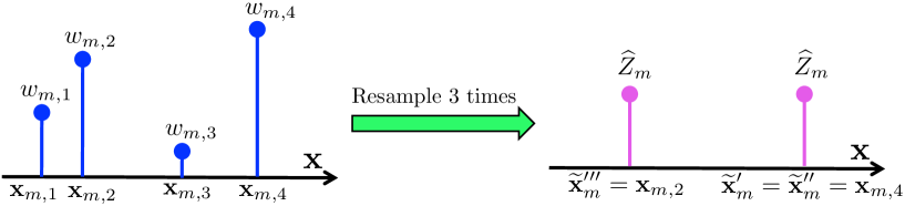
Figure 1: Example of generation (one run) and proper weighting of $3$ resampled particles (with replacement), $\widetilde{{\mathbf{x}}}_{m}^{\prime}$, $\widetilde{{\mathbf{x}}}_{m}^{\prime\prime}$ and $\widetilde{{\mathbf{x}}}_{m}^{\prime\prime\prime}$, from the $m$-th group, where $N_{m}=4$ and $\widehat{Z}_{m}=\frac{1}{4}\sum_{n=1}^{4}w_{m,n}$.

Definition 2.

The summary weight for the $m$-th group of samples is $W_{m}=N_{m}\widetilde{w}_{m}=N_{m}\widehat{Z}_{m}$.

Particle approximation.

Figure 2 represents graphically an example of GIS with $M=2$ and $N_{1}=4$, $N_{2}=3$. Given the $M$ summary pairs $\{\widetilde{{\mathbf{x}}}_{m},\widetilde{w}_{m}\}_{m=1}^{M}$ in a common computational node, we can obtain the following particle approximation of $\bar{\pi}({\mathbf{x}})$, i.e.,

$$\widehat{\pi}({\mathbf{x}}|\widetilde{{\mathbf{x}}}_{1:M})=\frac{1}{\sum_{j=1}^{M}N_{j}\widehat{Z}_{j}}\sum_{m=1}^{M}N_{m}\widehat{Z}_{m}\delta({\mathbf{x}}-\widetilde{{\mathbf{x}}}_{m}),$$ (13)

involving $M$ weighted samples in this case (see B). For a given function $h({\mathbf{x}})$, the corresponding specific GIS estimator in Eq. (10) is

$$\widetilde{I}_{M} = \frac{1}{\sum_{j=1}^{M}N_{j}\widehat{Z}_{j}}\sum_{m=1}^{M}N_{m}\widehat{Z}_{m}h(\widetilde{{\mathbf{x}}}_{m}).$$ (14)

It is a consistent estimator of $I$, as we show in B. The expression in Eq. (14) can be interpreted as a standard IS estimator where $\widetilde{w}(\widetilde{{\mathbf{x}}}_{m})=\widehat{Z}_{m}$ is a proper weight of a resampled particle (Martino et al., 2016a), and we give more importance to the resampled particles belonging to a set with higher cardinality. See DEMO-2 at https://github.com/lukafree/GIS.git.

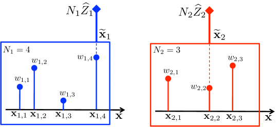
Figure 2: Graphical representation of GIS. In this case, $M=2$ groups of $N_{1}=4$ and $N_{2}=3$ weighted samples are summarized with a resampled particle and one summary weight $\widetilde{w}_{m}=N_{m}\widehat{Z}_{m}$, $m=1,2$.

Combination of estimators.

If we are only interested in computing the integral $I$ for a specific function $h({\mathbf{x}})$, we can summarize the statistical information by the pairs $\{{\overline{I}}_{N_{m}}^{(m)},\widetilde{w}_{m}\}$ where

$${\overline{I}}_{N_{m}}^{(m)}=\sum_{n=1}^{N_{m}}\bar{w}_{m,n}h({\mathbf{x}}_{m,n}),$$ (15)

is the $m$-th partial IS estimator obtained by using $N_{m}$ samples in $\mathcal{S}_{m}$. Given all the $S=\sum_{j=1}^{M}N_{j}$ weighted samples in the $M$ sets, the complete estimator ${\overline{I}}_{S}$ in Eq. (7) can be written as a convex combination of the $M$ partial IS estimators, ${\overline{I}}_{N_{m}}^{(m)}$, i.e.,

$${\overline{I}}_{S} = \frac{1}{\sum_{j=1}^{M}N_{j}\widehat{Z}_{j}}\sum_{m=1}^{M}\sum_{n=1}^{N_{m}}w_{m,n}h({\mathbf{x}}_{m,n}),$$ (16)

$$= \frac{1}{\sum_{j=1}^{M}N_{j}\widehat{Z}_{j}}\sum_{m=1}^{M}N_{m}\widehat{Z}_{m}\sum_{n=1}^{N_{m}}\bar{w}_{m,n}h({\mathbf{x}}_{m,n}),$$ (17)

$$= \frac{1}{\sum_{j=1}^{M}W_{m}}\sum_{m=1}^{M}W_{m}{\overline{I}}_{N_{m}}^{(m)}.$$ (18)

The equation above shows that the summary weight $W_{m}$ measures the importance of the $m$-th estimator ${\overline{I}}_{N_{m}}^{(m)}$. This confirms that $W_{m}$ is a proper weight the group of samples $\mathcal{S}_{m}$, and also suggests another valid compression scheme.

Remark 1.

In order to approximate only one specific moment $I$ of ${\bar{\pi}}({\mathbf{x}})$, we can summarize the $m$-group with the pair $\{{\overline{I}}_{N_{m}}^{(m)},W_{m}\}_{m=1}^{M}$, thus all the $M$ partial estimators can be combined following Eq. (18).

In this case, there is no loss of information w.r.t. storing all the weighted samples. However, the approximation of other moments of ${\bar{\pi}}({\mathbf{x}})$ is not possible. Figures 3-4 depict the graphical representations of the two possible approaches for GIS.

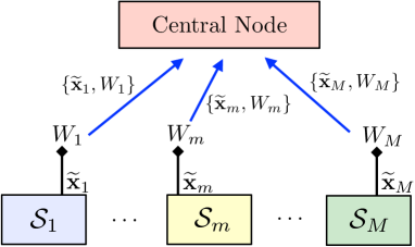
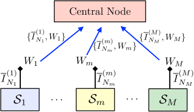
Figure 3: Graphical overview of GIS in a parallel/distributed framework. (a) The central node obtains all the pairs $\{\widetilde{{\mathbf{x}}}_{m},W_{m}\}_{m=1}^{M}$, and provides $\widehat{\pi}({\mathbf{x}}|\widetilde{{\mathbf{x}}}_{1:M})$ or ${\overline{I}}_{M}$. Note that only $M$ particles, $\widetilde{{\mathbf{x}}}_{m}\in\mathbb{R}^{D}$, and $M$ scalar weights, $W_{m}\in\mathbb{R}$, are transmitted, instead of $S$ samples and $S$ weights, with $S=\sum_{m=1}^{M}N_{m}$. (b) Alternatively, if we are interested only in a specific moment of the target, we can transmit the pairs $\{{\overline{I}}_{N_{m}}^{(m)},W_{m}\}_{m=1}^{M}$ and then combine them as in Eq. (18).

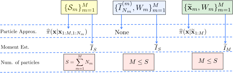
Figure 4: Possible outputs of different GIS compression schemes. On the left, $\{\mathcal{S}_{m}\}_{m=1}^{M}$, no compression is applied. In the center, $\{{\overline{I}}_{N_{m}}^{(m)},W_{m}\}_{m=1}^{M}$, we can perfectly reconstruct the estimator ${\overline{I}}_{S}$ in Eq. (16) where $S=\sum_{m=1}^{M}N_{m}$, but we cannot approximate other moments. Using $\{{\widetilde{{\mathbf{x}}}}_{N_{m}}^{(m)},W_{m}\}_{m=1}^{M}$, we always obtain a lossy compression, but any moments of ${\bar{\pi}}({\mathbf{x}})$ can be approximated, as shown in Eqs. (13)-(14).

4 GIS in other Monte Carlo schemes

4.1 Application in particle filtering

In Section 2.2, we have described the IS procedure in a batch way, i.e., generating directly a $D$-dimensional vector ${\bf x}^{\prime}\sim q({\mathbf{x}})$ and then compute the weight $\frac{\pi({\mathbf{x}}^{\prime})}{q({\mathbf{x}}^{\prime})}$. This procedure can be performed sequentially if the target density is factorized. In this case, the method is known as Sequential Importance Sampling (SIS). It is the basis of particle filtering, along with the use of the resampling procedure. Below, we describe the SIS method.

4.1.1 Sequential Importance Sampling (SIS)

Let us that recall ${\bf x}=x_{1:D}=[x_{1},x_{2},\ldots,x_{D}]\in\mathcal{X}\subseteq\mathbb{R}^{D\times\xi}$ where $x_{d}\in\mathbb{R}^{\xi}$ for all $d=1,\ldots,D$, and let us consider a target pdf $\bar{\pi}({\bf x})$ factorized as

$$\bar{\pi}({\bf x})=\frac{1}{Z}\pi({\bf x}) = \frac{1}{Z}\gamma_{1}(x_{1})\prod_{d=2}^{D}\gamma_{d}(x_{d}|x_{1:d-1}),$$ (19)

where $\gamma_{1}(x_{1})$ is a marginal pdf and $\gamma_{d}(x_{d}|x_{1:d-1})$ are conditional pdfs. We can also consider a proposal pdf decomposed in the same way, $q({\bf x})=q_{1}(x_{1})\prod_{d=2}^{D}q_{d}(x_{d}|x_{d-1})$. In a batch IS scheme, given the $n$-th sample ${\bf x}_{n}=x_{1:D}^{(n)}\sim q({\bf x})$, we assign the importance weight

$$w({\bf x}_{n}) = \frac{\pi({\bf x}_{n})}{q({\bf x}_{n})}=\frac{\gamma_{1}(x_{1}^{(n)})\gamma_{2}(x_{2}^{(n)}|x_{1}^{(n)})\cdots\gamma_{D}(x_{D}^{(n)}|x_{1:D-1}^{(n)})}{q_{1}(x_{1}^{(n)})q_{2}(x_{2}^{(n)}|x_{1}^{(n)})\cdots q_{D}(x_{D}^{(n)}|x_{1:D-1}^{(n)})}=\prod_{d=1}^{D}\beta_{d},$$ (20)

where $\beta_{1}^{(n)}=\frac{\pi(x_{1}^{(n)})}{q(x_{1}^{(n)})}$ and $\beta_{d}^{(n)}=\frac{\gamma_{d}(x_{d}^{(n)}|x_{1:d-1}^{(n)})}{q_{d}(x_{d}^{(n)}|x_{1:d-1}^{(n)})}$, with $d=2,\ldots,D$. Let us also denote the joint probability of $[x_{1},\ldots,x_{d}]$ as

$$\bar{\pi}_{d}(x_{1:d})=\frac{1}{Z_{d}}\pi_{d}(x_{1:d})=\frac{1}{Z_{d}}\gamma_{1}(x_{1})\prod_{j=2}^{d}\gamma_{j}(x_{j}|x_{1:j-1}),$$ (21)

where $Z_{d}=\int_{\mathbb{R}^{d\times\xi}}\pi_{d}(x_{1:d})dx_{1:d}$. Note that $\bar{\pi}_{D}(x_{1:D})\equiv\bar{\pi}({\bf x})$ and $Z_{D}\equiv Z$. Thus, we can draw samples generating sequentially each component $x_{d}^{(n)}\sim q_{d}(x_{d}|x_{1:d-1}^{(n)})$, $d=1,\ldots,D$, so that ${\mathbf{x}}_{n}=x_{1:D}^{(n)}\sim q({\bf x})=q_{1}(x_{1})\prod_{d=2}^{D}q_{d}(x_{d}|x_{d-1})$, and compute recursively the corresponding IS weight in Eq. (20). Indeed, considering the definition

$$w_{d}^{(n)}=\frac{\pi_{d}(x_{1:d}^{(n)})}{q_{1}(x_{1}^{(n)})\prod_{j=2}^{d}q_{j}(x_{j}^{(n)}|x_{1:j-1}^{(n)})}$$ (22)

we have the recursion $w_{d}^{(n)}=w_{d-1}^{(n)}\beta_{d}^{(n)}=\prod_{j=1}^{d}\beta_{j}^{(n)}$, with $w_{0}^{(n)}=1$, and we recall that $\beta_{d}^{(n)}=\frac{\gamma_{d}(x_{d}^{(n)}|x_{1:d-1}^{(n)})}{q_{d}(x_{d}^{(n)}|x_{1:d-1}^{(n)})}$. The SIS technique is also given in Table 3 by setting $\eta=0$. Note also that $\widehat{Z}_{d}=\frac{1}{N}\sum_{n=1}^{N}w_{d}^{(n)}$ is an unbiased estimator of $Z_{d}$. Defining the normalized weights ${\bar{w}}_{d}^{(n)}=\frac{w_{d}^{(n)}}{\sum_{i=1}^{N}w_{d}^{(i)}}$, in SIS we have another equivalent formulation of the same estimator as shown below.

Remark 2.

In SIS, there are two possible formulations of the estimator of the normalizing constant $Z_{d}=\int_{\mathbb{R}^{d\times\xi}}\pi_{d}(x_{1:d})dx_{1:d}$,

$$\widehat{Z}_{d} = \frac{1}{N}\sum_{n=1}^{N}w_{d}^{(n)}=\frac{1}{N}\sum_{n=1}^{N}w_{d-1}^{(n)}\beta_{d}^{(n)},$$ (23)

$$\overline{Z}_{d} = \prod_{j=1}^{d}\left[\sum_{n=1}^{N}{\bar{w}}_{j-1}^{(n)}\beta_{j}^{(n)}\right].$$ (24)

In SIS, both estimators are equivalent $\overline{Z}_{d}\equiv\widehat{Z}_{d}$. See C for further details.

4.1.2 Sequential Importance Resampling (SIR)

The expression in Eq. (20) suggests a recursive procedure for generating the samples and computing the importance weights, as shown in Steps 2a and 2b of Table 3. In Sequential Importance Resampling (SIR), a.k.a., standard particle filtering, resampling steps are incorporated during the recursion as in step 2(c)ii of Table 3 (Djurić et al., 2003; Doucet et al., 2001). In general, the resampling steps are applied only in certain iterations in order to avoid the path degeneration, taking into account an approximation $\widehat{ESS}$ of the Effective Sampling Size (ESS) (Huggins and Roy, 2015; Martino et al., 2017d). If $\widehat{ESS}$ is smaller than a pre-established threshold, the particles are resampled. Two examples of ESS approximation are $\widehat{ESS}=\frac{1}{\sum_{n=1}^{N}(\bar{w}_{d}^{(n)})^{2}}$ and $\widehat{ESS}=\frac{1}{\max\bar{w}_{d}^{(n)}}$ where $\bar{w}_{d}^{(n)}=\frac{w_{d}^{(n)}}{\sum_{i=1}^{N}w_{d}^{(i)}}$. Note that, in both cases, $1\leq\widehat{ESS}\leq N$. Hence, the condition for the adaptive resampling can be expressed as $\widehat{ESS}<\eta N$ where $\eta\in[0,1]$. SIS is given when $\eta=0$ and SIR for $\eta\in(0,1]$. When $\eta=1$, the resampling is applied at each iteration and in this case SIR is often called bootstrap particle filter (Djurić et al., 2003; Doucet et al., 2001; Doucet and Johansen, 2008). If $\eta=0$, no resampling is applied, we only apply Steps 2a and 2b, and we have the SIS method described above, that after $D$ iterations is completely equivalent to the batch IS approach, since $w_{n}=w({\bf x}_{n})\equiv w_{D}^{(n)}$ where ${\mathbf{x}}_{n}=x_{1:D}$.

Partial resampling.

In Table 3, we have considered that only a subset of $R\leq N$ particles are resampled. In this case, step 2(c)iii including the GIS weighting is strictly required in order to provide final proper weighted samples and hence consistent estimators. The partial resampling procedure is an alternative approach to prevent the loss of particle diversity (Martino et al., 2016a). In the classical description of SIR (Rubin, 1988), we have $R=N$ (i.e., all the particles are resampled) and the weight recursion follows setting the unnormalized weights of the resampled particles to any equal value. Since all the $N$ particles have been resampled, the selection of this value has no impact in the weight recursion and in the estimation of $I$.

Marginal likelihood estimators.

Even in the case $R=N$, i.e., all the particle are resampled as in the standard SIR method, without using the GIS weighting only the formulation $\overline{Z}_{d}$ in Eq. (24) provides a consistent estimator of $Z_{d}$, since it involves the normalized weights ${\bar{w}}_{d-1}^{(n)}$, instead of the unnormalized ones, $w_{d-1}^{(n)}$.

Remark 3.

If the GIS weighting is applied in SIR, both formulations $\widehat{Z}_{d}$ and $\overline{Z}_{d}$ in Eqs. (23)-(24) provide consistent estimator of $Z_{d}$ and they are equivalent, $\widehat{Z}_{d}\equiv\overline{Z}_{d}$ (as in SIS). See an exhaustive discussion in C.

See DEMO-1 at https://github.com/lukafree/GIS.git.

Table 3: SIR with partial resampling

1. Choose $N$ the number of particles, $R\leq N$ the number of particles to be resampled, the initial particles $x_{0}^{(n)}$, with $w_{0}^{(n)}=1$, $n=1,\ldots,N$, an ESS approximation $\widehat{ESS}$ (Martino et al., 2017d) and a constant value $\eta\in[0,1]$. 2. For $d=1,\ldots,D$: (a) Propagation: Draw $x_{d}^{(n)}\sim q_{d}(x_{d}|x_{1:d-1}^{(n)})$, for $n=1,\ldots,N$. (b) Weighting: Compute the weights $$w_{d}^{(n)}=w_{d-1}^{(n)}\beta_{d}^{(n)}=\prod_{j=1}^{d}\beta_{j}^{(n)},\quad\quad n=1,\ldots,N,$$ (25) where $\beta_{d}^{(n)}=\frac{\gamma_{d}(x_{d}^{(n)}|x_{1:d-1}^{(n)})}{q_{d}(x_{d}^{(n)}|x_{1:d-1}^{(n)})}$. (c) if $\widehat{ESS}<\eta N$ then: i. Select randomly, without repetition, a set of particles $\mathcal{S}=\{x_{1:d}^{(j_{r})}\}_{r=1}^{R}$ where $R\leq N$, $j_{r}\in\{1,\ldots,N\}$ for all $r$, and $j_{r}\neq j_{k}$ for $r\neq k$. ii. Resampling: Resample $R$ times within the set $\mathcal{S}$ according to the probabilities $\bar{w}_{d}^{(j_{r})}=\frac{w_{d}^{(j_{r})}}{\sum_{k=1}^{R}w_{d}^{(j_{k})}}$, obtaining $\{\bar{x}_{1:d}^{(j_{r})}\}_{r=1}^{R}$. Then, set $x_{1:d}^{(j_{r})}=\bar{x}_{1:d}^{(j_{r})}$, for $r=1,\ldots,R$. iii. GIS weighting: Compute $\widehat{Z}_{\mathcal{S}}=\frac{1}{R}\sum\limits_{r=1}^{R}w_{d}^{(j_{r})}$ and set $w_{d}^{(j_{r})}=\widehat{Z}_{\mathcal{S}}$ for all $r=1,\ldots,R$. 3. Return $\{{\mathbf{x}}_{n}=x_{1:D}^{(n)},w_{n}=w_{D}^{(n)}\}_{n=1}^{N}$.

GIS in Sequential Monte Carlo (SMC).

The idea of summary sample and summary weight have been implicitly used in different SMC schemes proposed in literature, for instance, for the communication among parallel particle filters (Bolić et al., 2005; Míguez and Vázquez, 2016; Read et al., 2014), and in the particle island methods (Verg et al., 2015, 2014; Whiteley et al., 2016). GIS also appears indirectly in particle filtering for model selection (Drovandi et al., 2014; Martino et al., 2017c; Urteaga et al., 2016) and in the so-called Nested Sequential Monte Carlo techniques (Naesseth et al., 2015, 2016; Stern, 2015).

4.2 Multiple Try Metropolis schemes as a Standard Metropolis-Hastings method

The Metropolis-Hastings (MH) method, described in Section 2.1, is a simple and popular MCMC algorithm (Liang et al., 2010; Liu, 2004; Robert and Casella, 2004). It generates a Markov chain $\{{\mathbf{x}}_{t}\}_{t=1}^{\infty}$ where $\bar{\pi}({\mathbf{x}})$ is the invariant density. Considering a proposal pdf $q({\mathbf{x}})$ independent from the previous state ${\mathbf{x}}_{t-1}$, the corresponding Independent MH (IMH) scheme is formed by the steps in Table 4 (Robert and Casella, 2004).

Table 4: The Independent Metropolis-Hastings (IMH) algorithm

1. Choose an initial state ${\mathbf{x}}_{0}$. 2. For $t=1,\ldots,T:$ (a) Draw a sample ${\mathbf{v}}^{\prime}\sim q({\mathbf{x}})$. (b) Accept the new state, ${\mathbf{x}}_{t}={\bf v}^{\prime}$, with probability $$\alpha({\mathbf{x}}_{t-1},{\bf v}^{\prime})=\min\left[1,\frac{\pi({\bf v}^{\prime})q({\mathbf{x}}_{t-1})}{\pi({\bf x}_{t-1})q({\bf v}^{\prime})}\right]=\min\left[1,\frac{w({\bf v}^{\prime})}{w({\bf x}_{t-1})}\right],$$ (26) where $w({\mathbf{x}})=\frac{\pi({\mathbf{x}})}{q({\mathbf{x}})}$ (standard importance weight). Otherwise, set ${\mathbf{x}}_{t}={\mathbf{x}}_{t-1}$. 3. Return $\{{\mathbf{x}}_{t}\}_{t=1}^{T}$.

Observe that $\alpha({\mathbf{x}}_{t-1},{\bf v}^{\prime})=\min\left[1,\frac{w({\bf v}^{\prime})}{w({\bf x}_{t-1})}\right]$ in Eq. (26) involves the ratio between the importance weight of the proposed sample ${\mathbf{v}}^{\prime}$ at the $t$-th iteration, and the importance weight of the previous state ${\mathbf{x}}_{t-1}$. Furthermore, note that at each iteration only one new sample ${\mathbf{v}}^{\prime}$ is generated and compared with the previous state ${\mathbf{x}}_{t-1}$ by the acceptance probability $\alpha({\mathbf{x}}_{t-1},{\bf v}^{\prime})$ (in order to obtain the next state ${\mathbf{x}}_{t}$). The Particle Metropolis-Hastings (PMH) method (Andrieu et al., 2010) and the alternative version of the Independent Multiply Try Metropolis technique (Martino et al., 2014b) (denoted as I-MTM2) are jointly described in Table 5. They are two MCMC algorithms where at each iteration several candidates $\{{\mathbf{v}}_{1},\ldots,{\mathbf{v}}_{N}\}$ are generated. After computing the IS weights $w({\mathbf{v}}_{n})$, one candidate is selected ${\mathbf{v}}_{j}$ within the $N$ possible values, i.e., $j\in\{1,\ldots,N\}$, applying a resampling step according to the probability mass $\bar{w}_{n}=\frac{w({\mathbf{v}}_{n})}{\sum_{i=1}^{N}w({\mathbf{v}}_{i})}=\frac{w({\mathbf{v}}_{n})}{N\widehat{Z}^{\prime}}$, $n=1,\ldots,N$. Then the selected sample ${\mathbf{v}}_{j}$ is tested with a proper probability $\alpha({\mathbf{x}}_{t-1},{\mathbf{v}}_{j})$ in Eq. (27).

Table 5: PMH and I-MTM2 techniques

1. Choose an initial state ${\mathbf{x}}_{0}$ and $\widehat{Z}_{0}$. 2. For $t=1,\ldots,T:$ (a) Draw $N$ particles ${\mathbf{v}}_{1},\ldots,{\mathbf{v}}_{N}$ from $q({\mathbf{x}})$ and weight them with the proper importance weight $w({\mathbf{v}}_{n})$, $n=1,\ldots,N$, using a sequential approach (PMH), or a batch approach (I-MTM2). Thus, denoting $\widehat{Z}^{\prime}=\frac{1}{N}\sum_{n=1}^{N}w({\mathbf{v}}_{n})$, we obtain the particle approximation $\widehat{\pi}({\mathbf{x}}|{\mathbf{v}}_{1:N})=\frac{1}{N\widehat{Z}^{\prime}}\sum_{n=1}^{N}w({\mathbf{v}}_{n})\delta({\mathbf{x}}-{\mathbf{v}}_{n})$. (b) Draw ${\mathbf{v}}_{j}\sim\widehat{\pi}({\mathbf{x}}|{\mathbf{v}}_{1:N})$. (c) Set ${\mathbf{x}}_{t}={\bf v}_{j}$ and $\widehat{Z}_{t}=\widehat{Z}^{\prime}$, with probability $$\alpha({\mathbf{x}}_{t-1},{\bf v}_{j})=\min\left[1,\frac{\widehat{Z}^{\prime}}{\widehat{Z}_{t-1}}\right].$$ (27) Otherwise, set ${\mathbf{x}}_{t}={\mathbf{x}}_{t-1}$ and $\widehat{Z}_{t}=\widehat{Z}_{t-1}$. 3. Return $\{{\mathbf{x}}_{t}\}_{t=1}^{T}$.

The difference between PMH and I-MTM2 is the procedure employed for the generation of the $N$ candidates and for the construction of the weights. PMH employs a sequential approach, whereas I-MTM2 uses a standard batch approach (Martino et al., 2014b). Namely, PMH generates sequentially the components $v_{j,k}$ of the candidates, ${\mathbf{v}}_{j}=[v_{j,1},\ldots,v_{j,D}]^{\top}$, and compute recursively the weights as shown in Section 4.1. Since resampling steps are often used, then the resulting candidates ${\mathbf{v}}_{1},\ldots,{\mathbf{v}}_{N}$ are correlated, whereas in I-MTM2 they are independent. I-MTM2 coincides with PMH if the candidates are generated sequentially but without applying resampling steps, so that I-MTM2 can be considered a special case of PMH.

Note that $\widetilde{w}({\bf v}_{j})=\widehat{Z}^{\prime}$ and $\widetilde{w}({{\mathbf{x}}}_{t-1})=\widehat{Z}_{t-1}$ are the GIS weights of the resampled particles ${\bf v}_{j}$ and ${\mathbf{x}}_{t-1}$ respectively, as stated in Definition 1 and Theorem 1. Hence, considering the GIS theory, we can write

$$\alpha({\mathbf{x}}_{t-1},{\bf v}_{j})=\min\left[1,\frac{\widehat{Z}^{\prime}}{\widehat{Z}_{t-1}}\right]=\min\left[1,\frac{\widetilde{w}({\bf v}_{j})}{\widetilde{w}({{\mathbf{x}}}_{t-1})}\right],$$ (28)

which has the form of the acceptance function of the classical IMH method in Table 4. Therefore, PMH and I-MTM2 algorithms can be also summarized as in Table 6.

Table 6: Alternative description of PMH and I-MTM2

1. Choose an initial state ${\mathbf{x}}_{0}$. 2. For $t=1,\ldots,T:$ (a) Draw $\widetilde{{\mathbf{x}}}^{\prime}\sim\widetilde{q}({\bf x})$, where $$\widetilde{q}({\bf x})=\int_{\mathcal{X}^{N}}\left[\prod_{i=1}^{N}q({\bf v}_{i})\right]\widehat{\pi}({\bf x}|{\bf v}_{1:N})d{\bf v}_{1:N},$$ (29) is the equivalent proposal pdf associated to a resampled particle (Lamberti et al., 2016; Martino et al., 2016a). (b) Set ${\mathbf{x}}_{t}=\widetilde{{\mathbf{x}}}^{\prime}$, with probability $$\alpha({\mathbf{x}}_{t-1},\widetilde{{\mathbf{x}}}^{\prime})=\min\left[1,\frac{\widetilde{w}(\widetilde{{\mathbf{x}}}^{\prime})}{\widetilde{w}({\mathbf{x}}_{t-1})}\right].$$ (30) Otherwise, set ${\mathbf{x}}_{t}={\mathbf{x}}_{t-1}$. 3. Return $\{{\mathbf{x}}_{t}\}_{t=1}^{T}$.

Remark 4.

The PMH and I-MTM2 algorithms take the form of the classical IMH method employing the equivalent proposal pdf $\widetilde{q}({\bf x})$ in Eq. (29) (depicted in Figure 5; see also A), and using the GIS weight $\widetilde{w}(\widetilde{{\mathbf{x}}}^{\prime})$ of a resampled particle $\widetilde{{\mathbf{x}}}^{\prime}\sim\widetilde{q}({\bf x})$, within the acceptance function $\alpha({\mathbf{x}}_{t},\widetilde{{\mathbf{x}}}^{\prime})$.

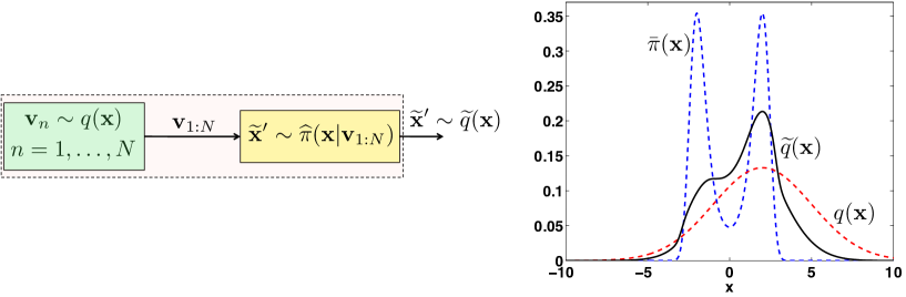
Figure 5: (Left) Graphical representation of the generation of one sample ${\bf x}^{\prime}$ from the equivalent proposal pdf $\widetilde{q}({\bf x})$ in Eq. (29).(Right) Example of the equivalent density $\widetilde{q}({\bf x})$ (solid line) with $N=2$. The target, $\bar{\pi}({\mathbf{x}})$, and proposal, $q({\mathbf{x}})$, pdfs are shown with dashed lines. See DEMO-3 at https://github.com/lukafree/GIS.git.

5 Novel MCMC techniques based on GIS

In this section, we provide two examples of novel MCMC algorithms based on GIS. First of all, we introduce a Metropolis-type method producing a chain of sets of weighted samples. Secondly, we present a PMH technique driven by $M$ parallel particle filters. In the first scheme, we exploit the concept of summary weight and all the weighted samples are stored. In the second one, both concepts of summary weight and summary particle are used. The consistency of the resulting estimators and the ergodicity of both schemes is ensured and discussed.

5.1 Group Metropolis Sampling

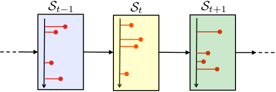
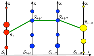
Figure 6: (a) Chain of sets $\mathcal{S}_{t}=\{{\mathbf{x}}_{n,t},\rho_{n,t}\}_{n=1}^{N}$ generated by the GMS method (graphical representation with $N=4$). (b) Graphical examples of GMS outputs, $\mathcal{S}_{t}$, $\mathcal{S}_{t+1}$, $\mathcal{S}_{t+2}$ and $\mathcal{S}_{t+3}$, where $\mathcal{S}_{t+2}=\mathcal{S}_{t+1}$. The weights of the samples are denoted by the size of the circles. A possible recovered MTM chain is also depicted with solid line, where the states are ${\bf\widetilde{x}}_{\tau}$ with $\tau=t,t+1,t+2,t+3$ and ${\bf\widetilde{x}}_{t+2}={\bf\widetilde{x}}_{t+1}$.

Here, we describe an MCMC procedure that yields a sequence of sets of weighted samples. All the samples are then employed for a joint particle approximation of the target distribution. The Group Metropolis Sampling (GMS) is outlined in Table 7. Figures 6(a)-(b) give two graphical representations of GMS outputs $\mathcal{S}_{t}=\{{\mathbf{x}}_{n,t}={\mathbf{v}}_{n},\rho_{n,t}=w_{n}\}_{n=1}^{N}$ (with $N=4$ in both cases). Note that the GMS algorithm uses the idea of summary weight for comparing sets. Let us denote as $\rho_{n,t}$ the importance weights assigned to the samples ${\mathbf{x}}_{n,t}$ contained in the current set $\mathcal{S}_{t}$. Given the generated sets $\mathcal{S}_{t}=\{{\mathbf{x}}_{n,t},\rho_{n,t}\}_{n=1}^{N}$, for $t=1,\ldots,T$, GMS provides the global particle approximation

$$\widehat{\pi}({\mathbf{x}}|{\mathbf{x}}_{1:N,1:T}) = \frac{1}{T}\sum_{t=1}^{T}\sum_{n=1}^{N}\frac{\rho_{n,t}}{\sum_{i=1}^{N}\rho_{i,t}}\delta({\mathbf{x}}-{\mathbf{x}}_{n,t}),$$ (31)

$$= \frac{1}{T}\sum_{t=1}^{T}\sum_{n=1}^{N}\bar{\rho}_{n,t}\delta({\mathbf{x}}-{\mathbf{x}}_{n,t}),$$ (32)

where $\bar{\rho}_{n,t}=\frac{\rho_{n,t}}{\sum_{i=1}^{N}\rho_{i,t}}$. Thus, the estimator of a specific moment of the target is

$$\widetilde{I}_{NT}=\frac{1}{T}\sum_{t=1}^{T}\sum_{n=1}^{N}\bar{\rho}_{n,t}h({\mathbf{x}}_{n,t})=\sum_{n=1}^{N}\bar{\rho}_{n,t}\widetilde{I}_{T}^{(n)}=\frac{1}{T}\sum_{t=1}^{T}\widetilde{I}_{N}^{(t)},$$ (33)

where we have denoted

$$\widetilde{I}_{T}^{(n)}=\frac{1}{T}\sum_{t=1}^{T}h({\mathbf{x}}_{n,t}),\quad\widetilde{I}_{N}^{(t)}=\sum_{n=1}^{N}\bar{\rho}_{n,t}h({\mathbf{x}}_{n,t}).$$ (34)

See also E for further details. If the $N$ candidates at step 2a, ${\mathbf{v}}_{1},\ldots,{\mathbf{v}}_{N}$, and the associated weights, $w_{1},\ldots,w_{N}$, are built sequentially by a particle filtering method, we have a Particle GMS (PGMS) algorithm (see Section 6.4) and marginal versions can be also considered (see D).

Table 7: Group Metropolis Sampling

1. Build an initial set $\mathcal{S}_{0}=\{{\mathbf{x}}_{n,0},\rho_{n,0}\}_{n=1}^{N}$ and $\widehat{Z}_{0}=\frac{1}{N}\sum_{n=1}^{N}\rho_{n,0}$. 2. For $t=1,\ldots,T:$ (a) Draw $N$ samples, ${\mathbf{v}}_{1},\ldots,{\mathbf{v}}_{N}\sim q({\bf x})$ following a sequential or a batch procedure. (b) Compute the weights, $w_{n}=\frac{\pi({\mathbf{v}}_{n})}{q({\mathbf{v}}_{n})}$, $n=1,\dots,N$; define $\mathcal{S}^{\prime}=\{{\mathbf{v}}_{n},w_{n}\}_{n=1}^{N}$; and compute $\widehat{Z}^{\prime}=\frac{1}{N}\sum_{n=1}^{N}w_{n}$. (c) Set $\mathcal{S}_{t}=\{{\mathbf{x}}_{n,t}={\mathbf{v}}_{n},\rho_{n,t}=w_{n}\}_{n=1}^{N}$, i.e., $\mathcal{S}_{t}=\mathcal{S}^{\prime}$, and $\widehat{Z}_{t}=\widehat{Z}^{\prime}$, with probability $$\alpha(\mathcal{S}_{t-1},\mathcal{S}^{\prime})=\min\left[1,\frac{\widehat{Z}^{\prime}}{\widehat{Z}_{t-1}}\right].$$ (35) Otherwise, set $\mathcal{S}_{t}=\mathcal{S}_{t-1}$ and $\widehat{Z}_{t}=\widehat{Z}_{t-1}$. 3. Return $\{\mathcal{S}_{t}\}_{t=1}^{T}$, or $\{\widetilde{I}_{N}^{(t)}\}_{t=1}^{T}$ where $\widetilde{I}_{N}^{(t)}=\sum\limits_{n=1}^{N}\frac{\rho_{n,t}}{\sum_{i=1}^{N}\rho_{i,t}}h({\mathbf{x}}_{n,t})$.

Relationship with IMH.

The acceptance probability $\alpha$ in Eq. (35) is the extension of the acceptance probability of IMH in Eq. (26), by considering the proper GIS weighting of a set of weighted samples. Note that, in this version of GMS, all the sets contain the same number of samples.

Relationship with MTM methods.

GMS is strictly related to Multiple Try Metropolis (MTM) schemes (Casarin et al., 2013; Martino et al., 2012; Martino and Read, 2013; Martino et al., 2014b) and Particle Metropolis Hastings (PMH) techniques (Andrieu et al., 2010; Martino et al., 2014b). The main difference is that GMS uses no resampling steps at each iteration for generating summary samples, indeed GMS uses the entire set. However, considering a sequential of a batch procedure for generating the $N$ tries at each iteration, we can recover an MTM (or the PMH) chain by the GMS output applying one resampling step when $\mathcal{S}_{t}\neq\mathcal{S}_{t-1}$,

$$\widetilde{{\mathbf{x}}}_{t}=\left\{\begin{split}&\widetilde{{\mathbf{v}}}_{t}\sim\sum_{n=1}^{N}\bar{\rho}_{n,t}\delta({\mathbf{x}}-{\mathbf{x}}_{n,t}),\quad\quad\mbox{ if }\quad\mathcal{S}_{t}\neq\mathcal{S}_{t-1},\\ &\widetilde{{\mathbf{x}}}_{t-1},\quad\quad\quad\quad\quad\quad\quad\quad\quad\mbox{ }\mbox{ if }\quad\mathcal{S}_{t}=\mathcal{S}_{t-1},\end{split}\right.$$ (36)

for $t=1,\ldots,T$. Namely, $\{\widetilde{{\mathbf{x}}}_{t}\}_{t=1}^{T}$ is the chain obtained by one run of the MTM (or PMH) technique. Figure 6(b) provides a graphical representation of a MTM chain recovered by GMS outputs.

Ergodicity.

As also discussed above, (a) the sample generation, (b) the acceptance probability function and hence (c) the dynamics of GMS exactly coincides with the corresponding steps of PMH or MTM (with a sequential or batch particle generation, respectively). Hence, the ergodicity of the chain is ensured (Casarin et al., 2013; Martino and Read, 2013; Andrieu et al., 2010; Martino et al., 2014b). Indeed, we can recover the MTM (or PMH) chain as shown in Eq. (LABEL:RecChain).

Recycling samples.

The GMS algorithm can be seen as a method of recycling auxiliary weighted samples in MTM schemes (or PMH schemes, if the candidates are generated by SIR). However, GMS does not recycle all the samples generated at the step 2a of Table 7. Indeed, when a set is rejected, GMS discards these samples and repeats the previous set. Therefore, GMS also decides which samples will be either recycled or not. In (Casella and Robert, 1996), the authors show how recycling and including the samples rejected in one run of a standard MH method into a unique consistent estimator. GMS can be considered an extension of this technique where $N\geq 1$ candidates are drawn at each iteration.

Iterated IS.

GMS can be also interpreted as an iterative importance sampling scheme where an IS approximation of $N$ samples is built at each iteration and compared with the previous IS approximation. This procedure is iterated $T$ times and all the accepted IS estimators $\widetilde{I}_{N}^{(t)}$ are finally combined to provide a unique global approximation of $NT$ samples. Note that the temporal combination of the IS estimators is obtained dynamically by the random repetitions due to the rejections in the MH test. Hence, the complete procedure for weighting the samples generated by GMS can be interpreted as the composition of two weighting schemes: (a) by an importance sampling approach building $\{\rho_{n,t}\}_{n=1}^{N}$ and (b) by the possible random repetitions due to the rejections in the MH-type test.

Connection with dynamic weighting schemes.

For its hybrid nature between an IS method and a MCMC technique, GMS could recall the dynamic weighting schemes proposed in (Wong and Liang, 1997). The authors in (Wong and Liang, 1997) have proposed different kinds of moves considering weighted samples, that are suitable according to the so-called “invariance with respect to the importance weights” condition. However, these moves are completely different from the GMS scheme. The dynamic of GMS is totally based on standard ergodic theory, indeed, we can recover a standard MCMC chain from the GMS output, as shown in Eq. (LABEL:RecChain).

Consistency of the GMS estimator.

Recovering the MTM chain $\{\widetilde{{\mathbf{x}}}_{t}\}_{t=1}^{T}$ as in Eq. (LABEL:RecChain), the estimator obtained by the recovered chain, $\widetilde{I}_{T}=\frac{1}{T}\sum_{t=1}^{T}h(\widetilde{{\mathbf{x}}}_{t})$, is consistent. Namely, $\widetilde{I}_{T}$ converges almost-surely to $I=E_{\bar{\pi}}[h({\mathbf{x}})]$ as $T\rightarrow\infty$, since $\{\widetilde{{\mathbf{x}}}_{t}\}_{t=1}^{T}$ is an ergodic chain (Robert and Casella, 2004). For $\mathcal{S}_{t}\neq\mathcal{S}_{t-1}$, note that $E_{\widehat{\pi}}[h(\widetilde{{\mathbf{x}}}_{t})|\mathcal{S}_{t}]=\sum_{n=1}^{N}\bar{\rho}_{n,t}h({\mathbf{x}}_{n,t})=\widetilde{I}_{N}^{(t)}$ in Eq. (34), where $\widehat{\pi}({\mathbf{x}}|{\mathbf{x}}_{1:N,t})=\sum_{n=1}^{N}\bar{\rho}_{n,t}\delta({\mathbf{x}}-{\mathbf{x}}_{n,t})$. If $\mathcal{S}_{t}=\mathcal{S}_{t-1}$, then $E_{\widehat{\pi}}[h(\widetilde{{\mathbf{x}}}_{t})|\mathcal{S}_{t}]=E_{\widehat{\pi}}[h(\widetilde{{\mathbf{x}}}_{t-1})|\mathcal{S}_{t-1}]=\widetilde{I}_{N}^{(t-1)}$ and, since $\widetilde{I}_{N}^{(t)}=\widetilde{I}_{N}^{(t-1)}$, we have again $E_{\widehat{\pi}}[h(\widetilde{{\mathbf{x}}}_{t})|\mathcal{S}_{t}]=\widetilde{I}_{N}^{(t)}$. Therefore, we have

$$E[\widetilde{I}_{T}|\mathcal{S}_{1:T}] = \frac{1}{T}\sum_{t=1}^{T}E_{\widehat{\pi}}[h(\widetilde{{\mathbf{x}}}_{t})|\mathcal{S}_{t}]$$ (37)

$$= \frac{1}{T}\sum_{t=1}^{T}\widetilde{I}_{N}^{(t)}=\widetilde{I}_{NT},$$ (38)

whee the last equality comes from Eq. (33). Thus, the GSM estimator $\widetilde{I}_{NT}$ in Eq. (33) can be expressed as $\widetilde{I}_{NT}=E[\widetilde{I}_{T}\big{|}\mathcal{S}_{1:T}]$, where $\mathcal{S}_{1:T}$ represents all the weighted samples obtained by GMS and $\widetilde{I}_{T}=\frac{1}{T}\sum_{t=1}^{T}h(\widetilde{{\mathbf{x}}}_{t})$ is the estimator obtained by a given MTM chain recovered by using Eq. (LABEL:RecChain). Hence, $\widetilde{I}_{NT}$ is consistent for $T\rightarrow\infty$ since $\widetilde{I}_{T}$ is consistent, owing to the MTM chain is ergodic. Furthermore, fixing $T$, the GMS estimator $\widetilde{I}_{NT}$ in Eq. (33) is also consistent when $N\rightarrow\infty$, due to the standard IS arguments (Liu, 2004). The consistency can be also shown considering GMS as the limit case of an in finite number of recovered parallel IMTM2 chains, as in Eq. (LABEL:RecChain), as shown in E.

5.2 Distributed Particle Metropolis-Hastings algorithm

The PMH algorithm is an MCMC technique particularly designed for filtering and smoothing a dynamic variable in a state-space model (Andrieu et al., 2010; Martino et al., 2014b) (see for instance Figure 12). In PMH, different trajectories obtained by different runs of a particle filter (see Section 4.1) are compared according to suitable MH-type acceptance probabilities, as shown in Table 5. In this section, we show how several parallel particle filters (for instance, each one consider a different proposal pdf) can drive a PMH-type technique.

The classical PMH method uses a single proposal pdf $q({\mathbf{x}})=q_{1}(x_{1})\prod_{d=2}^{D}q_{d}(x_{d}|x_{1:d-1})$, employed in single SIR method in order to generate new candidates before of the MH-type test (see Table 5). Let us consider the problem of tracking a variable of interest ${\mathbf{x}}=[x_{1},\ldots,x_{D}]^{\top}\in\mathbb{R}^{D\times\xi}$ with target pdf $\pi({\mathbf{x}})=\pi_{1}(x_{1})\prod_{d=2}^{D}\pi_{d}(x_{d}|x_{1:d-1})$. We assume that $M$ independent processing units are available jointly with a central node as shown Fig. 7. We use $M$ parallel particle filters, each one with a different proposal pdf, $q_{m}({\mathbf{x}})=q_{m,1}(x_{1})\prod_{d=2}^{D}q_{m,d}(x_{d}|x_{1:d-1})$, one per each processor. Then, after one run of the parallel particle filters, we obtain $M$ particle approximations $\widehat{\pi}_{m}({\mathbf{x}})$. Since, we aim to reduce the communication cost to the central node (see Figs. 3 and 7), we consider that each machine only transmits the pair $\{\widehat{Z}_{m},\widetilde{{\mathbf{x}}}_{m}\}$, where $\widetilde{{\mathbf{x}}}_{m}\sim\widehat{\pi}_{m}({\mathbf{x}})$ (we set $N_{1}=\ldots=N_{M}$, for simplicity). Applying the GIS theory, then it is straightforward to outline the method, called Distributed Particle Metropolis-Hastings (DPMH) technique, shown in Table 8.

Table 8: Distributed Particle Metropolis-Hastings algorithm

1. Choose an initial state ${\mathbf{x}}_{0}$ and $\widehat{Z}_{m,0}$ for $m=1,\ldots,M$ (e.g., both obtained with a first run of a particle filter). 2. For $t=1,\ldots,T:$ (a) (Parallel Processors) Draw $N$ particles ${\mathbf{v}}_{m,1},\ldots,{\mathbf{v}}_{m,N}$ from $q_{m}({\mathbf{x}})$ and weight them with IS weights $w({\mathbf{v}}_{m,n})$, $n=1,\ldots,N$, using a particle filter (or a batch approach), for each $m=1,\ldots,M$. Thus, denoting $\widehat{Z}_{m}=\frac{1}{N}\sum_{n=1}^{N}w({\mathbf{v}}_{m,n})$, we obtain the $M$ particle approximations $\widehat{\pi}_{m}({\mathbf{x}})=\widehat{\pi}({\mathbf{x}}|{\mathbf{v}}_{m,1:N})=\frac{1}{N\widehat{Z}_{m}}\sum_{n=1}^{N}w({\mathbf{v}}_{m,n})\delta({\mathbf{x}}-{\mathbf{v}}_{m,n})$. (b) (Parallel Processors) Draw $\widetilde{{\mathbf{x}}}_{m}\sim\widehat{\pi}({\mathbf{x}}|{\mathbf{v}}_{m,1:N})$, for $m=1,\ldots,M$. (c) (Central Node) Resample $\widetilde{{\mathbf{x}}}\in\{\widetilde{{\mathbf{x}}}_{1},\ldots,\widetilde{{\mathbf{x}}}_{M}\}$ according to the pmf $\frac{\widehat{Z}_{m}}{\sum_{j=1}^{M}\widehat{Z}_{j}}$, $m=1,\ldots,M$, i.e., $\widetilde{{\mathbf{x}}}\sim\widehat{\pi}({\bf x}|\widetilde{{\mathbf{x}}}_{1},\ldots,\widetilde{{\mathbf{x}}}_{M})$. (d) (Central Node) Set ${\mathbf{x}}_{t}=\widetilde{{\mathbf{x}}}$ and $\widehat{Z}_{m,t}=\widehat{Z}_{m}$, for $m=1,\ldots,M$, with probability $$\alpha({\mathbf{x}}_{t-1},\widetilde{{\mathbf{x}}})=\min\left[1,\frac{\sum_{m=1}^{M}\widehat{Z}_{m}}{\sum_{m=1}^{M}\widehat{Z}_{m,t-1}}\right].$$ (39) Otherwise, set ${\mathbf{x}}_{t}={\mathbf{x}}_{t-1}$ and $\widehat{Z}_{m,t}=\widehat{Z}_{m,t-1}$, for $m=1,\ldots,M$.

The method in Table 8 has the structure of a Multiple Try Metropolis (MTM) algorithm using different proposal pdfs (Casarin et al., 2013; Martino and Read, 2013). More generally, in step 2a, the scheme described above can even employ different kinds of particle filtering algorithms. In step 2b, $M$ total resampling steps are performed,one per processor. Then, one resampling step is performed in the central node (step 2c). Finally, the resampled particle is accepted as new state with probability $\alpha$ in Eq. (39).

Ergodicity.

The ergodicity of DPMH is ensured since it can be interpreted as a standard PMH method considering a single particle approximation

$$\widehat{\pi}({\mathbf{x}}|{\mathbf{v}}_{1:M,1:N})=\sum_{m=1}^{M}\frac{\widehat{Z}_{m}}{\sum_{j=1}^{M}\widehat{Z}_{j}}\widehat{\pi}({\mathbf{x}}|{\mathbf{v}}_{m,1:N})=\sum_{m=1}^{M}\overline{W}_{m}\widehat{\pi}({\mathbf{x}}|{\mathbf{v}}_{m,1:N}),$$ (40)

and then we resample once, i.e., draw $\widetilde{{\mathbf{x}}}\sim\widehat{\pi}({\mathbf{x}}|{\mathbf{v}}_{1:M,1:N})$. Then, the proper weight of this resampled particle is $\widehat{Z}=\frac{1}{M}\sum_{m=1}^{M}\widehat{Z}_{m}$, so that the acceptance function of the equivalent classical PMH method is $\alpha({\mathbf{x}}_{t-1},\widetilde{{\mathbf{x}}})=\min\left[1,\frac{\widehat{Z}}{\widehat{Z}_{t-1}}\right]=\min\left[1,\frac{\frac{1}{M}\sum_{m=1}^{M}\widehat{Z}_{m}}{\frac{1}{M}\sum_{m=1}^{M}\widehat{Z}_{m,t-1}}\right]$, where $\widehat{Z}_{t-1}=\frac{1}{M}\sum_{m=1}^{M}\widehat{Z}_{m,t-1}$ (see Table 5).

Using partial IS estimators.

If we are interested in approximating only one moment of the target pdf, as shown in Figures 3-4, at each iteration we can transmit the $M$ partial estimators $\overline{I}_{N}^{(m)}$ and combine them in the central node as in Eq. (18), obtaining $\widetilde{I}_{NM}^{\prime}=\frac{1}{\sum_{j=1}^{M}\widehat{Z}_{j}}\sum_{m=1}^{M}\widehat{Z}_{m}{\overline{I}}_{N}^{(m)}$. Then, a sequence of estimators, $\widetilde{I}_{NM}^{(t)}$, is created according to the acceptance probability $\alpha$ in Eq. (39). Finally, we obtain the global estimator

$$\widetilde{I}_{NMT}=\frac{1}{T}\sum_{t=1}^{T}\widetilde{I}_{NM}^{(t)}.$$ (41)

This scheme is depicted in Figure 7(b).

Benefits.

The main advantage of the DPMH scheme is that the generation of samples can be parallelized (i.e., fixing the computational cost, DPMH allows the use of $M$ processors in parallel) and the communication to the central node requires the transfer of only $M$ particles, $\widetilde{{\mathbf{x}}}_{m}^{\prime}$, and $M$ weights, $\widehat{Z}_{m}^{\prime}$, instead of $NM$ particles and $NM$ weights. Figure 7 provides a general sketch of DPMH. Its marginal version is described in D. Another benefit of DPMH is that different types of particle filters can be jointly employed, for instance, different proposal pdfs can be used.

Special cases and extensions.

The classical PMH method is as a special case of the proposed algorithm of Table 8 when $M=1$. If the partial estimators are transmitted to the central node, as shown in Figure 7(b), DPMH coincides with PGMS when $M=1$. Adaptive versions of DPMH can be designed in order select automatically the best proposal pdf among the $M$ densities, based of the weights $\overline{W}_{m}=\frac{\widehat{Z}_{m}}{\sum_{j=1}^{M}\widehat{Z}_{j}}$, $m=1,\ldots,M$. For instance, Figure 13(b) shows that DPMH is able to detect the best scale parameters within the $M$ used values.

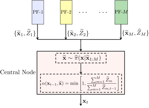
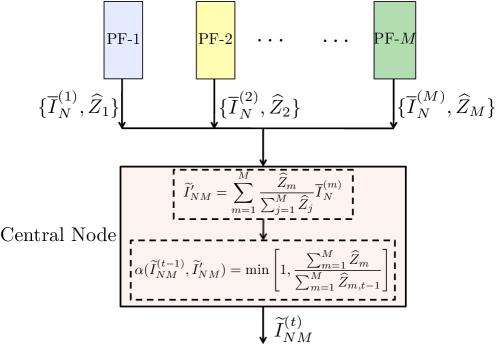
Figure 7: Graphical representation of Distributed Particle Metropolis-Hastings (DPMH) method, (a) for estimating a generic moment, or (b) for estimating of a specific moment of the target.

6 Numerical Experiments

In this section, we test the novel techniques considering several experimental scenarios and three different applications: hyperparameters estimation for Gaussian Processes ($D=2$), two different localization problems, and the online filtering of a remote sensing variable called Leaf Area Index (LAI; $D=365$). We compare the novel algorithms with different benchmark methods such adaptive MH algorithm, MTM and PMH techniques, parallel MH chains with random walk proposal pdfs, IS schemes, and the Adaptive Multiple Importance Sampling (AMIS) method.

6.1 Hyperparameter tuning for Gaussian Process (GP) regression models

We test the proposed GMS approach for the estimation of hyperparameters of a Gaussian process (GP) regression model (Bishop, 2006), (Rasmussen and Williams, 2006). Let us assume observed data pairs $\{y_{j},{\bf z}_{j}\}_{j=1}^{P}$, with $y_{j}\in\mathbb{R}$ and ${\bf z}_{j}\in\mathbb{R}^{L}$. We also denote the corresponding $P\times 1$ output vector as ${\bf y}=[y_{1},\ldots,y_{P}]^{\top}$ and the $L\times P$ input matrix as ${\bf Z}=[{\bf z}_{1},\ldots,{\bf z}_{P}]$. We address the regression problem of inferring the unknown function $f$ which links the variable $y$ and ${\bf z}$. Thus, the assumed model is $y=f({\bf z})+e$, where $e\sim N(e;0,\sigma^{2})$, and that $f({\bf z})$ is a realization of a GP (Rasmussen and Williams, 2006). Hence $f({\bf z})\sim\mathcal{GP}(\mu({\bf z}),\kappa({\bf z},{\bf r}))$ where $\mu({\bf z})=0$, ${\bf z},{\bf r}\in\mathbb{R}^{L}$, and we consider the kernel function

$$\kappa({\bf z},{\bf r})=\exp\left(-\sum_{\ell=1}^{L}\frac{(z_{\ell}-r_{\ell})^{2}}{2\delta^{2}}\right).$$ (42)

Given these assumptions, the vector ${\bf f}=[f({\bf z}_{1}),\ldots,f({\bf z}_{P})]^{\top}$ is distributed as $p({\bf f}|{\bf Z},\delta,\kappa)=\mathcal{N}({\bf f};{\bf 0},{\bf K})$, where ${\bf 0}$ is a $P\times 1$ null vector, and ${\bf K}_{ij}:=\kappa({\bf z}_{i},{\bf z}_{j})$, for all $i,j=1,\ldots,P$, is a $P\times P$ matrix. Therefore, the vector containing all the hyperparameters of the model is ${\mathbf{x}}=[\delta,\sigma]$, i.e., all the parameters of the kernel function in Eq. (42) and standard deviation $\sigma$ of the observation noise. In this experiment, we focus on the marginal posterior density of the hyperparameters, ${\bar{\pi}}({\mathbf{x}}|{\bf y},{\bf Z},\kappa)\propto\pi({\mathbf{x}}|{\bf y},{\bf Z},\kappa)=p({\bf y}|{\mathbf{x}},{\bf Z},\kappa)p({\mathbf{x}})$, which can be evaluated analytically, but we cannot compute integrals involving it (Rasmussen and Williams, 2006). Considering a uniform prior within $[0,20]^{2}$, $p({\mathbf{x}})$ and since $p({\bf y}|{\mathbf{x}},{\bf Z},\kappa)=\mathcal{N}({\bf y};{\bf 0},{\bf K}+\sigma^{2}{\bf I})$, we have

$$\begin{split}\log\left[\pi({\mathbf{x}}|{\bf y},{\bf Z},\kappa)\right]=-\frac{1}{2}{\bf y}^{\top}({\bf K}+\sigma^{2}{\bf I})^{-1}{\bf y}-\frac{1}{2}\log\left[\mbox{det}\left({\bf K}+\sigma^{2}{\bf I}\right)\right],\end{split}$$ (43)

where clearly ${\bf K}$ depends on $\delta$ (Rasmussen and Williams, 2006). The moments of this marginal posterior cannot be computed analytically. Then, in order to compute the Minimum Mean Square Error (MMSE) estimator $\widehat{{\mathbf{x}}}=[\widehat{\delta},\widehat{\sigma}]$, i.e., the expected value $E[{\bf X}]$ with ${\bf X}\sim{\bar{\pi}}({\mathbf{x}}|{\bf y},{\bf Z},\kappa)$, we approximate $E[{\bf X}]$ via Monte Carlo quadrature. More specifically, we apply a the novel GMS technique and compare with an MTM sampler, a MH scheme with a longer chain and a static IS method. For all these methodologies, we consider the same number of target evaluations, denoted as $E$, in order to provide a fair comparison.

We generated $P=200$ pairs of data, $\{y_{j},{\bf z}_{j}\}_{j=1}^{P}$, according to the GP model above setting $\delta^{*}=3$, $\sigma^{*}=10$, $L=1$, and drawing $z_{j}\sim\mathcal{U}([0,10])$. We keep fixed these data over the different runs, and the corresponding posterior pdf is given in Figure 9(b). We computed the ground-truth $\widehat{{\mathbf{x}}}=[\widehat{\delta}=3.5200,\widehat{\sigma}=9.2811]$ using an exhaustive and costly grid approximation, in order to compare the different techniques. For both GMS, MTM and MH schemes, we consider the same adaptive Gaussian proposal pdf $q_{t}({\bf x}|{\bm{\mu}}_{t},\lambda^{2}{\bf I})=\mathcal{N}({\bf x}|{\bm{\mu}}_{t},\lambda^{2}{\bf I})$, with $\lambda=5$ and ${\bm{\mu}}_{t}$ is adapted considering the arithmetic mean of the outputs after a training period, $t\geq 0.2T$, in the same fashion of (Haario et al., 2001) (${\bm{\mu}}_{0}=[1,1]^{\top}$). First, we test both techniques fixing $T=20$ and varying the number of tries $N$. Then, we set $N=100$ and vary the number of iterations $T$. Figure 8 (log-log plot) shows the Mean Square Error (MSE) in the approximation of $\widehat{{\mathbf{x}}}$ averaged over $10^{3}$ independent runs. Observe that GMS always outperforms the corresponding MTM scheme. These results confirm the advantage of recycling the auxiliary samples drawn at each iteration during an MTM run. In Figure 9(a), we show the MSE obtained by GMS keeping invariant the number of target evaluations $E=NT=10^{3}$ and varying $N\in\{1,2,10,20,50,100,250,10^{3}\}$. As a consequence, we have $T\in\{10^{3},500,100,50,20,10,4,1\}$. Note that the case $N=1$, $T=10^{3}$, corresponds to an adaptive MH (A-MH) method with a longer chain, whereas the case $N=10^{3}$, $T=1$, corresponds to a static IS scheme (both with the same posterior evaluations $E=NT=10^{3}$). We observe that the GMS always provides smaller MSE than the static IS approach. Moreover, GMS outperforms A-MH with the exception of two cases where $T\in\{1,4\}$.

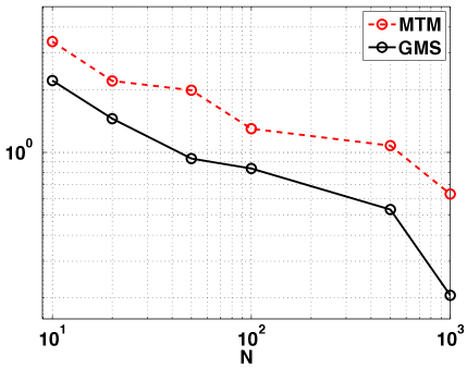
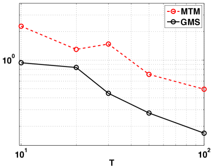
Figure 8: MSE (loglog-scale; averaged over $10^{3}$ independent runs) obtained with the MTM and GMS algorithms (using the same proposal pdf and the same values of $N$ and $T$) (a) as function of $N$ with $T=20$ and (b) as function of $T$ with $N=100$.

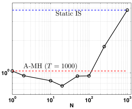
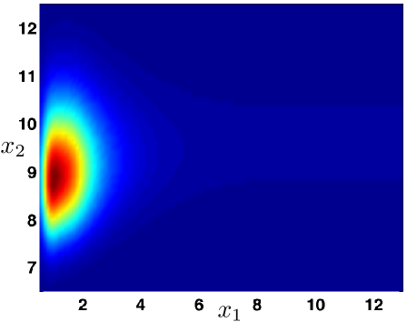
Figure 9: (a) MSE (loglog-scale; averaged over $10^{3}$ independent runs) of GMS (circles) versus the number of candidates $N\in\{1,2,10,20,50,100,250,10^{3}\}$, but keeping fixed the total number of posterior evaluations $E=NT=1000$, so that $T\in\{1000,500,100,50,20,10,4,1\}$. The MSE values the extreme cases $N=1$, $T=1000$, and $N=1000$, $T=1$, are depicted with dashed lines. In first case, GMS coincides with an adaptive MH scheme (due the adaptation of the proposal, in this example) with a longer chain. The second one represents a static IS scheme (clearly, using the sample proposal than GMS). We can observe the benefit of the dynamic combination of IS estimators obtained by GMS. (b) Posterior density $\pi({\mathbf{x}}|{\bf y},{\bf Z},\kappa)$.

6.2 Localization of a target and tuning of the sensor network

We consider the problem of positioning a target in $\mathbb{R}^{2}$ using a range measurements in a wireless sensor network (Ali et al., 2007; Ihler et al., 2005). We also assume that the measurements are contaminated by noise with different unknown power, one per each sensor. This situation is common in several practical scenarios. Actually, even if the sensors have the same construction features, the noise perturbation of each the sensor can vary with the time and depends on the location of the sensor. This occurs owing to different causes: manufacturing defects, obstacles in the reception, different physical environmental conditions (such as humidity and temperature) etc. Moreover, in general, these conditions change along time, hence it is necessary that the central node of the network is able to re-estimate the noise powers jointly with position of the target (and other parameters of the models if required) whenever a new block of observations is processed. More specifically, let us denote the target position with the random vector $\textbf{Z}=[Z_{1},Z_{2}]^{\top}$. The position of the target is then a specific realization ${\bf Z}={\bf z}$. The range measurements are obtained from $N_{S}=6$ sensors located at $\textbf{h}_{1}=[3,-8]^{\top}$, $\textbf{h}_{2}=[8,10]^{\top}$, $\textbf{h}_{3}=[-4,-6]^{\top}$, $\textbf{h}_{4}=[-8,1]^{\top}$, $\textbf{h}_{5}=[10,0]^{\top}$ and $\textbf{h}_{6}=[0,10]^{\top}$ as shown in Figure 10(a). The observation models are given by

$$\begin{split}Y_{j}=20\log\left(||{\bf z}-{\bf h}_{j}||\right)+B_{j},\quad j=1,\ldots,N_{S},\\ \end{split}$$ (44)

where $B_{j}$ are independent Gaussian random variables with pdfs, $\mathcal{N}(b_{j};0,\lambda_{j}^{2})$, $j=1,\ldots,N_{S}$. We denote ${\bm{\lambda}}=[\lambda_{1},\ldots,\lambda_{N_{S}}]$ the vector of standard deviations. Given the position of the target ${\bf z}^{*}=[z_{1}^{*}=2.5,z_{2}^{*}=2.5]^{\top}$ and setting ${\bm{\lambda}}^{*}=[\lambda_{1}^{*}=1,\lambda_{2}^{*}=2,\lambda_{3}^{*}=1,\lambda_{4}^{*}=0.5,\lambda_{5}^{*}=3,\lambda_{6}^{*}=0.2]$ (since $N_{S}=6$), we generate $N_{O}=20$ observations from each sensor according to the model in Eq. (44). Then, we finally obtain a measurement matrix ${\bf Y}=[y_{k,1},\ldots,y_{k,N_{S}}]\in\mathbb{R}^{d_{Y}}$, where $d_{Y}=N_{O}N_{S}=120$, $k=1,\ldots,N_{O}$. We consider uniform prior $\mathcal{U}(\mathcal{R}_{z})$ over the position $[z_{1},z_{2}]^{\top}$ with $\mathcal{R}_{z}=[-30\times 30]^{2}$, and a uniform prior over $\lambda_{j}$, so that ${\bm{\lambda}}$ has prior $\mathcal{U}(\mathcal{R}_{\lambda})$ with $\mathcal{R}_{\lambda}=[0,20]^{N_{S}}$. Thus, the posterior pdf is

$${\bar{\pi}}({\bf x}|\textbf{Y})={\bar{\pi}}({\bf z},{\bm{\lambda}}|\textbf{Y})=\ell(\textbf{y}|z_{1},z_{2},\lambda_{1},\ldots,\lambda_{N_{S}})\prod_{i=1}^{2}p(z_{i})\prod_{j=1}^{N_{S}}p(\lambda_{j}),$$ (45)

$$= \left[\prod_{k=1}^{N_{O}}\prod_{j=1}^{N_{S}}\frac{1}{\sqrt{2\pi\lambda_{j}^{2}}}\exp\left(-\frac{1}{2\lambda_{j}^{2}}(y_{k,j}+10\log\left(||{\bf z}-{\bf h}_{j}||\right)^{2}\right)\right]\mathbb{I}_{z}(\mathcal{R}_{z})\mathbb{I}_{\lambda}(\mathcal{R}_{\lambda}),$$ (46)

where ${\bf x}=[{\bf z},{\bm{\lambda}}]^{\top}$ is a vector of parameters of dimension $D=N_{S}+2=8$ that we desire to infer, and $\mathbb{I}_{c}(\mathcal{R})$ is an indicator variable that is $1$ if $c\in\mathcal{R}$, otherwise is $0$.

Our goal is to compute the Minimum Mean Square Error (MMSE) estimator, i.e., the expected value of the posterior ${\bar{\pi}}({\bf x}|\textbf{Y})={\bar{\pi}}({\bf z},{\bm{\lambda}}|\textbf{Y})$. Since the MMSE estimator cannot be computed analytically, we apply Monte Carlo methods for approximating it. We compare GMS, the corresponding MTM scheme, the Adaptive Multiple Importance Sampling (AMIS) technique (Cornuet et al., 2012), and $N$ parallel MH chains with a random walk proposal pdf. For all of them we consider Gaussian proposal densities. For GMS and MTM, we set $q_{t}({\bf x}|{\bm{\mu}}_{t},\sigma^{2}\mathbb{I})=\mathcal{N}({\bf x}|{\bm{\mu}}_{t},\sigma^{2}\mathbb{I})$ where ${\bm{\mu}}_{t}$ is adapted considering the empirical mean of the generated samples after a training period, $t\geq 0.2T$ (Haario et al., 2001), ${\bm{\mu}}_{0}\sim\mathcal{U}([1,5]^{D})$ and $\sigma=1$. For AMIS, we have $q_{t}({\bf x}|{\bm{\mu}}_{t},{\bf C}_{t})=\mathcal{N}({\bf x}|{\bm{\mu}}_{t},{\bf C}_{t})$, where ${\bm{\mu}}_{t}$ is as previously described (with ${\bm{\mu}}_{0}\sim\mathcal{U}([1,5]^{D})$) and ${\bf C}_{t}$ is also adapted using the empirical covariance matrix, starting ${\bf C}_{0}=4{\bf I}$. We also test the use of $N$ parallel Metropolis-Hastings (MH) chains (we also consider the case of $N=1$, i.e., a single chain), with a Gaussian random-walk proposal pdf, $q_{n}({\bm{\mu}}_{n,t}|{\bm{\mu}}_{n,t-1},\sigma^{2}{\bf I})=\mathcal{N}({\bm{\mu}}_{n,t}|{\bm{\mu}}_{n,t-1},\sigma^{2}{\bf I})$ with ${\bm{\mu}}_{n,0}\sim\mathcal{U}([1,5]^{D})$ for all $n$ and $\sigma=1$.

We fix the total number of evaluations of the posterior density as $E=NT=10^{4}$. Note that, generally, the evaluation of the posterior is the most costly step in MC algorithms (however, AMIS has the additional cost of re-weighting all the samples at each iteration according to the deterministic mixture procedure (Bugallo et al., 2015; Cornuet et al., 2012; Elvira et al., 2015a)). We recall that $T$ denotes the total number of iterations and $N$ the number of samples drawn from each proposal at each iteration. We consider ${\bf x}^{*}=[{\bf z}^{*},{\bm{\lambda}}^{*}]^{\top}$ as the ground-truth and compute the Mean Square Error (MSE) in the estimation obtained with the different algorithms. The results are averaged over $500$ independent runs and they are provided in Tables 9, 10, and 11 and Figure 10(b). Note that GMS outperforms AMIS for each a pair $\{N,T\}$ (keeping fixed $E=NT=10^{4}$), and GMS also provides smaller MSE values than $N$ parallel MH chains (the case $N=1$ corresponds to a unique longer chain). Figure 10(b) shows the MSE versus $N$ maintaining $E=NT=10^{4}$ for GMS and the corresponding MTM method. This figure again confirms the advantage of recycling the samples in a MTM scheme.

Table 9: Results GMS.

MSE	1.30	1.24	1.22	1.21	1.22	1.19	1.31	1.44
$N$	10	20	50	100	200	500	1000	2000
$T$	1000	500	200	100	50	20	10	5
$E$	$NT=10^{4}$
MSE range	Min MSE= 1.19  ———  Max MSE= 1.44

Table 10: Results AMIS (Cornuet et al., 2012).

MSE	1.58	1.57	1.53	1.48	1.42	1.29	1.48	1.71
$N$	10	20	50	100	200	500	1000	2000
$T$	1000	500	200	100	50	20	10	5
$E$	$NT=10^{4}$
MSE range	Min MSE= 1.29  ———  Max MSE= 1.71

Table 11: Results $N$ parallel MH chains with random-walk proposal pdf.

MSE	1.42	1.31	1.44	2.32	2.73	3.21	3.18	3.15
$N$	1	5	10	50	100	500	1000	2000
$T$	$10^{4}$	2000	1000	200	100	20	10	5
$E$	$NT=10^{4}$
MSE range	Min MSE= 1.31  ———  Max MSE=3.21

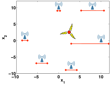
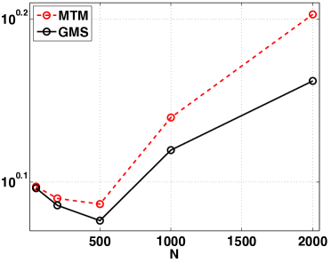
Figure 10: (a) Sensor network: the location of the sensors (antennas) and the target (circle) in the numerical example. The solid line represents the different unknown variances of the sensors. (b) MSE (log-scale) versus the number of candidates $N\in\{50,200,500,1000,2000\}$ obtained by GMS and the corresponding MTM algorithm, keeping fixed the total number of evaluations $E=NT=10^{4}$ of the posterior pdf, so that $T\in\{200,50,20,10,5\}$.

6.3 Target localization with real data

In this section, we test the proposed techniques in real data application. More specifically, we consider again a positioning problem in order to localize a target in a bidimensional space using range measurements (Ali et al., 2007; Patwari et al., 2003).

6.3.1 Setup of the Experiment

We have designed a network of four nodes. Three of them are placed at fixed positions and play the role of sensors that measure the strength of the radio signals transmitted by the target. The other node plays the role of the target to be localized. All nodes are bluetooth devices (Conceptronic CBT200U2A) with a nominal maximum range of 200 m. The deployment of the network is given in Figure 11(a). We consider a square monitored area of $4\times 4$ m and place the sensors at fixed positions $\textbf{h}_{1}=[h_{1,1}=0.5,h_{1,2}=1]$, $\textbf{h}_{2}=[h_{2,1}=3.5,h_{2,2}=1]$ and $\textbf{h}_{3}=[h_{3,1}=2,h_{3,2}=3]$, with all coordinates in meters. The target is located at $\textbf{p}=[p_{1}=2.5,p_{2}=2]$.

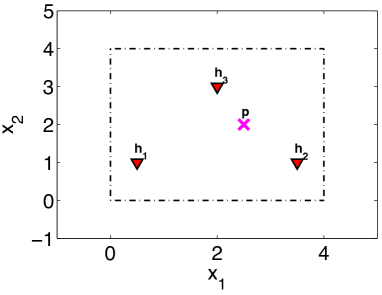
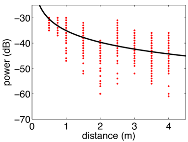
Figure 11: (a) Experimental setup: sensors over a rectangular surveillance area of 4 times 4 meters. The sensors are shown with triangles (denoted by ${\bf h}_{i}$) while the target that must be localized is depicted with a cross (denoted by ${\bf p}$). (b) The least squares regression to adjust the parameters $l$ and $\gamma$. The points indicate the measurements collected by the sensors at different distances, and the solid curve denotes the function $\hat{l}-10\hat{\gamma}\log\left[\frac{d}{d_{0}}\right]$ with $d_{0}=0.3$, $\hat{l}=-27.08$ dB and $\hat{\gamma}=1.52$.

The measurement equation describes the relationship between the observed radio signal strength $y_{i}$ obtained by the $i$-th sensor, and the target position $\textbf{p}=[p_{1},p_{2}]$ (see (Rappaport, 2001)), and is given by

$$y_{i}=l-10\gamma\log\left[\frac{\sqrt{(p_{1}-h_{i,1})^{2}+(p_{2}-h_{i,2})^{2}}}{d_{0}}\right]+\theta_{i}\ \ \ \ \mbox{(dB)},$$ (47)

where $\gamma$ is a parameter that depends on the physical environment (for instance, in an open space $\gamma\approx 2$), and the constant $l$ is the mean power received by each sensor when the target is located at a reference distance $d_{0}$. The measurement noise is Gaussian, $N(\theta_{i};0,\sigma^{2})\propto\exp\left\{-\frac{\theta_{i}^{2}}{2\sigma^{2}}\right\}$ with $i=1,2,3$. In this experiment, the reference distance has been set to $d_{0}=0.3$ m. Unlike in the previous numerical example, here the parameters $l$, $\gamma$, and $\sigma^{2}$ have been tuned in advance by least square regression using $200$ measurements with the target placed at known distances from each sensor. As a result, we have obtained $\hat{l}=-27.08$, $\hat{\gamma}=1.52$, and $\hat{\sigma}=4.41$. Figure 11(b) shows the measurements obtained at several distances and the fitted curve $\hat{l}-10\hat{\gamma}\log\left[\frac{d}{d_{0}}\right]$, where $d=\sqrt{(p_{1}-h_{i,1})^{2}+(p_{2}-h_{i,2})^{2}}$.

6.3.2 Posterior density, algorithms and results

Assume we collect $M$ independent measurements from each sensor, considering the observation model in Eq. (47). Let $\textbf{y}=[y_{1,1},\ldots,y_{1,M},y_{2,1},\ldots,y_{2,M},y_{3,1},\ldots,y_{3,M}]$ denote the measurement vector where $y_{i,j}$ is the $j$-th observation of the $i$-th sensor. The the likelihood is

$$\small\begin{split}p(\textbf{y}|\textbf{p})=\prod_{i=1}^{3}\prod_{m=1}^{M}\mathcal{N}\left(y_{i,m}|\hat{l}-10\hat{\gamma}\log\right(||\textbf{p}-\textbf{h}_{i}||/d_{0}\left),\hat{\sigma}^{2}\right),\quad{\bf p}\in[0,4]\times[0,4].\end{split}$$ (48)

We set $p(\textbf{y}|\textbf{p})=0$ if ${\bf p}\notin[0,4]\times[0,4]$. We assume a Gaussian prior for each component of ${\bf p}$ with mean $1.5$ and variance $0.5$. Hence, the posterior density is given by $p(\textbf{p}|\textbf{y})\propto p(\textbf{y}|\textbf{p})p(\textbf{p})$ where $p(\textbf{p})$ denotes the bidimensional Gaussian prior pdf over the position ${\bf p}$. Our goal is to approximate the expected value of the posterior $p(\textbf{p}|\textbf{y})$. We collect $M=10$ measurements from each Conceptronic CBT200U2A devices, and compute the ground-truth (i.e., the expected value) with a costly determinist grid. Then, we apply GMS and the corresponding MTM scheme, considering the same bidimensional proposal density $q({\bf p}|{\bm{\mu}},\lambda^{2}\mathbb{I})=\mathcal{N}({\bf p}|{\bm{\mu}},\lambda^{2}\mathbb{I})$ where ${\bm{\mu}}\sim\mathcal{U}([0,4]\times[0,4])$ (randomly chosen at each independent run) and $\lambda=\sqrt{2}$. We set $N=50$ and $T=100$. We compute the Mean Square Error (MSE) with respect to the ground-truth obtained with GMS and MTM, in $500$ different independent runs. The averaged MSE values are $1.81$ for the GMS method and $2.2$ for the MTM scheme. Therefore, GMS outperforms the corresponding MTM technique also in this experiment.

6.4 Tracking of biophysical parameters

We consider the challenging problem of estimating biophysical parameters from remote sensing (satellite) observations. In particular, we focus on the estimation of the Leaf Area Index (LAI). It is important to track evolution of LAI through time in every spatial position on Earth because LAI plays an important role in vegetation processes such as photosynthesis and transpiration, and is connected to meteorological/climate and ecological land processes (Chen and Black, 1992). Let us denote LAI as $x_{d}\in\mathbb{R}^{+}$ (where $d\in\mathbb{N}^{+}$ also represents a temporal index) in a specific region at a latitude of $42^{\circ}$ N (Gomez-Dans et al., 2016). Since $x_{t}>0$, we consider Gamma prior pdfs over the evolutions of LAI and Gaussian perturbations for the “in-situ” received measurements, $y_{t}$. More specifically, we assume the state-space model (formed by propagation and measurement equations),

$$\left\{\begin{array}[]{lll}g_{d}(x_{d}|x_{d-1})&=\mathcal{G}\left(x_{d}\Big{|}\frac{x_{d-1}}{b},b\right)&=\frac{1}{c_{d}}x_{d}^{(x_{d-1}-b)/b}\exp\left(-\frac{x_{d}}{b}\right),\\ \ell_{d}(y_{d}|x_{d})&=\mathcal{N}(y_{d}|x_{d},\lambda^{2})&=\frac{1}{\sqrt{2\pi\lambda^{2}}}\exp\left(-\frac{1}{2\lambda^{2}}(y_{d}-x_{d})^{2}\right),\end{array}\right.$$ (49)

for $d=2,\ldots,D$, with initial probability $g_{1}(x_{1})=\mathcal{G}(x_{1}|1,1)$, where $b,\lambda>0$ and $c_{d}>0$ is a normalizing constant. Note that the expected value of the Gamma pdf above is $x_{d-1}$ and the variance is $b$.

First Experiment.

Considering that all the parameters of the model are known, the posterior pdf is

$$\bar{\pi}({\mathbf{x}}|{\mathbf{y}}) \propto \ell({\mathbf{y}}|{\mathbf{x}})g({\mathbf{x}})=\left[\prod_{d=2}^{D}\ell_{d}(y_{d}|x_{d})\right]\left[\left(\prod_{d=2}^{D}g_{d}(x_{d}|x_{d-1})\right)g_{1}(x_{1})\right],$$ (50)

with ${\mathbf{x}}=x_{1:D}\in\mathbb{R}^{D}$. For generating the ground-truth (i.e., the trajectory ${\mathbf{x}}^{*}=x_{1:D}^{*}=[x_{1}^{*},\ldots,x_{D}^{*}]$), we simulate the temporal evolution of LAI in one year (i.e., $1\leq d\leq D=365$) by using a double logistic function (as suggested in the literature (Gomez-Dans et al., 2016)), i.e.,

$$x_{d}=a_{1}+a_{2}\left(\frac{1}{1+\exp(a_{3}(d-a_{4}))}+\frac{1}{1+\exp(a_{5}(d-a_{6}))}+1\right),$$ (51)

with $a_{1}=0.1$, $a_{2}=5$, $a_{3}=-0.29$, $a_{4}=120$, $a_{5}=0.1$ and $a_{6}=240$ as employed in (Gomez-Dans et al., 2016). In Figure 12, the true trajectory $x_{1:D}$ is depicted with dashed lines. The observations ${\mathbf{y}}=y_{2:D}$ are then generated (each run) according to $y_{d}\sim\ell_{d}(y_{d}|x_{d})=\frac{1}{\sqrt{2\pi\lambda^{2}}}\exp\left(-\frac{1}{2\lambda^{2}}(y_{d}-x_{d})^{2}\right)$. First of all, we test the standard PMH, the particle version of GMS (PGMS), and DPMH (fixing $\lambda=0.1$). For DPMH, we use $M=4$ parallel filters with different scale parameters ${\bf b}=[b_{1}=0.01,b_{2}=0.05,b_{3}=0.1,b_{4}=1]^{\top}$. Figure 12 shows the estimated trajectories $\widehat{{\mathbf{x}}}_{t}=\widehat{x}_{1:D,t}=\frac{1}{t}\sum_{\tau=1}^{t}\widetilde{{\mathbf{x}}}_{\tau}$ (averaged over 2000 runs) obtained by DPMH with $N=5$ at $t\in\{2,10,100\}$, in one specific run. Figure 13(a) depicts the evolution of the MSE obtained by DPMH as a function of $T$ and considering different values of $N\in\{5,7,10,20\}$. The performance of DPMH improves as $T$ and $N$ grow, as expected. DPMH detects the best parameters among the four values in ${\bf b}$, following the weights $\overline{W}_{m}$ (see Figure 13(b)) and DPMH takes advantage of this ability. Indeed, we compare DPMH with $N=10$, $T=200$, and $M=4$ using ${\bf b}$, with $M=4$ different standard PMH and PGMS algorithms with $N=40$ and $T=200$ (clearly, each one driven by a unique filter, $M=1$) in order to keep the total number of evaluation of the posterior fixed, $E=NMT=8\cdot 10^{3}$, each one using a parameter $b_{m}$, $m=1,\ldots,M$. The results, averaged over 2000 runs, are shown in Table 12. In terms of MSE, DPMH always outperforms the $4$ possible standard PMH methods. PGMS using two parameters, $b_{2}$ and $b_{3}$, provides better performance, but DPMH outperforms PGMS averaging the $4$ different MSEs obtained by PGMS. Moreover, due to the parallelization, in this case DPMH can save $\approx 15\%$ of the spent computational time.

Second Experiment.

Now we consider also the parameter $\lambda$ unknown, so that the complete variable of interest $[{\mathbf{x}},\lambda]\in\mathbb{R}^{D+1}$. Then the posterior is $\bar{\pi}({\mathbf{x}},\lambda|{\mathbf{y}})\propto\ell({\mathbf{y}}|{\mathbf{x}},\lambda)g({\mathbf{x}},\lambda)$ according to the model Eq. (49), where $g({\mathbf{x}},\lambda)=g({\mathbf{x}})g_{\lambda}(\lambda)$ and $g_{\lambda}(\lambda)$ is a uniform pdf in $[0.01,5]$. Then we test the marginal versions of the PMH and DPMH with $q_{\lambda}(\lambda)=g_{\lambda}(\lambda)$ (see D), for estimating $[{\mathbf{x}}^{*},\lambda^{*}]$ where ${\mathbf{x}}^{*}=x_{1:D}^{*}$ is given by Eq. (51) and $\lambda^{*}=0.7$. Figure 14 shows the MSE in estimation of $\lambda^{*}$ (averaged over 1000 runs) obtained by DPMMH as function of $T$ and different number of candidates, $N\in\{5,10,20\}$ (with again $M=4$ and ${\bf b}=[b_{1}=0.01,b_{2}=0.05,b_{3}=0.1,b_{4}=1]^{\top}$). Table 13 compares the standard PMMH and DPMMH for estimating $\lambda^{*}$ (we set $E=NMT=4\cdot 10^{3}$ and $T=100$). Averaging the results of PMMH, we can observe that DPMMH outperforms the standard PMMH in terms of smaller MSE and smaller computational time.

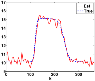
(a) $t=2$

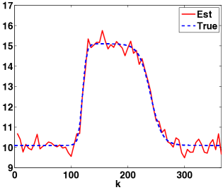
(b) $t=10$

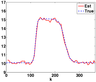
(c) $t=100$

Figure 12: Output of DPMH (with $N=5$, $\lambda=0.1$ and ${\bf b}=[0.01,0.05,0.1,1]^{\top}$) at different iterations (a) $t=2$, (b) $t=10$, and (c) $t=100$, in one specific run. The true values, ${\mathbf{x}}^{*}=x_{1:D}^{*}$, are shown dashed lines whereas the estimated trajectories by DPMH, $\widehat{{\mathbf{x}}}_{t}=\widehat{x}_{1:D,t}$, with solid lines.

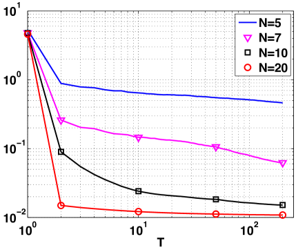
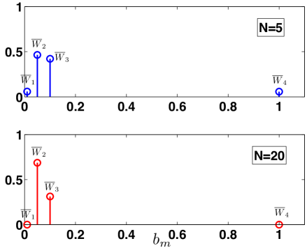
Figure 13: (a) MSE in estimation of the trajectory (averaged over $2000$ runs) obtained by DPMH as function $T$ and different values of $N\in\{5,7,10,20\}$. As expected, we can see that the performance of DPMH improves as $T$ and $N$ grow. (b) Averaged values of the normalized weights $\overline{W}_{m}=\frac{\widehat{Z}_{m}}{\sum_{j=1}^{M}\widehat{Z}_{j}}$ (with $N=5$ and $N=10$) associated to each filter. DPMH is able to detect the best variances ($b_{2}$ and $b_{3}$) of the proposal pdfs among the values $b_{1}=0.01$, $b_{2}=0.05$, $b_{3}=0.1$ and $b_{4}=1$ (as confirmed by Table 12).

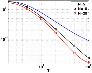
Figure 14: MSE in estimation of $\lambda^{*}=0.7$ (averaged over $1000$ runs) obtained by DPMMH as function $T$ and different values of $N\in\{5,10,20\}$.

Table 12: Comparison among PMH, PGMS and DPMH with $E=NMT=8\cdot 10^{3}$ and $T=200$ ($\lambda=0.1$), estimating the trajectory ${\mathbf{x}}^{*}=x_{1:D}^{*}$.

Proposal Var	Standard PMH	PGMS	DPMH
	$N=40$	$N=40$	$N=10$
	$(M=1)$	$(M=1)$	$M=4$
	MSE	MSE	MSE
$b_{1}=0.01$	0.0422	0.0380	0.0108
$b_{2}=0.05$	0.0130	0.0100
$b_{3}=0.1$	0.0133	0.0102
$b_{4}=1$	0.0178	0.0140
Average	0.0216	0.0181	0.0108
Norm. Time	1	1	0.83

Table 13: Comparison among PMMH and DMPMH with $E=NMT=4\cdot 10^{3}$ and $T=100$, for estimating $\lambda^{*}=0.7$.

Proposal Var	PMMH	DPMMH
	$N=40$	$N=10$
	$(M=1)$	$M=4$
	MSE	MSE
$b_{1}=0.01$	0.0929	0.0234
$b_{2}=0.05$	0.0186
$b_{3}=0.1$	0.0401
$b_{4}=1$	0.0223
Average	0.0435	0.0234
Norm. Time	1	0.85

7 Conclusions

In this work, we have described the Group Importance Sampling (GIS) theory and its application in other Monte Carlo schemes. We have considered the use of GIS in SIR (a.k.a., particle filtering), showing that GIS is strictly required if the resampling procedure is applied only in a subset of the current population of particles. Moreover we have highlighted that, in the standard SIR method, if GIS is applied there exists two equivalent estimators of the marginal likelihood (one of them is an estimator of the marginal likelihood only if the GIS weighting is used), exactly as in Sequential Importance Sampling (SIS). We have also shown that the Independent Multiple Try Metropolis (I-MTM) schemes and the Particle Metropolis-Hastings (PMH) algorithm can be interpreted as a classical Metropolis-Hastings (MH) method taking into account the GIS approach.

Furthermore, two novel methodologies based on GIS have been introduced. One of them (GMS) yields a Markov chain of weighted samples and can be also considered an iterative importance sampler. The second one (DPMH) is a distributed version of the PMH where different parallel particle filters can be jointly employed. These filter cooperate for driving the PMH scheme. Both techniques have been applied successfully in three different numerical experiments (tuning of the hyperparameters for GPs, two localization problems in a wireless sensor network (one with real data), and the tracking of the Leaf Area Index), comparing them with several benchmark methods. Marginal versions of GMS and DPMH have been also discussed and tested in the numerical applications. Three Matlab demos have been also given in order to facilitate the comprehension of the reader. As a future line, we plan to design an adaptive DPMH scheme in order to select online the best particle filters among the $M$ run in parallel, and parsimoniously distribute the computational effort.

Appendix A Proper weighting of a resampled particle

Let us consider the particle approximation of $\bar{\pi}$ obtained by the IS approach drawing $N$ particles ${\bf x}_{n}\sim q({\mathbf{x}})$, $n=1\ldots,N$, i.e.,

$$\widehat{\pi}({\bf x}|{\bf x}_{1:N})=\sum_{n=1}^{N}{\bar{w}}({\bf x}_{n})\delta({\bf x}-{\bf x}_{n})=\sum_{n=1}^{N}\frac{w({\bf x}_{n})}{\sum_{i=1}^{N}w({\bf x}_{i})}\delta({\bf x}-{\bf x}_{n})=\frac{1}{N\widehat{Z}}\sum_{n=1}^{N}w({\bf x}_{n})\delta({\bf x}-{\bf x}_{n}).$$ (52)

where

$$\widehat{Z}=\widehat{Z}({\bf x}_{1:N})=\frac{1}{N}\sum_{i=1}^{N}w({\bf x}_{i}).$$ (53)

Given the set of particles ${\bf x}_{1:N}\sim\prod_{n=1}^{N}q({\mathbf{x}}_{n})$, a resampled particle is generated as $\widetilde{{\mathbf{x}}}^{\prime}\sim\widehat{\pi}({\bf x}|{\bf x}_{1:N})$. Let us denote the joint pdf $\widetilde{Q}({\bf x},{\bf x}_{1:N})=\widehat{\pi}({\bf x}|{\bf x}_{1:N})\left[\prod_{i=1}^{N}q({\bf x}_{i})\right]$. The marginal pdf $\widetilde{q}({\bf x})$ of a resampled particle $\widetilde{{\mathbf{x}}}^{\prime}$, integrating out ${\bf x}_{1:N}$ (i.e., $\widetilde{{\mathbf{x}}}^{\prime}\sim\widetilde{q}({\bf x})$), is

$$\widetilde{q}({\bf x}) = \int_{\mathcal{X}^{N}}\widetilde{Q}({\bf x},{\bf x}_{1:N})d{\bf x}_{1:N}$$ (54)

$$= \int_{\mathcal{X}^{N}}\widehat{\pi}({\bf x}|{\bf x}_{1:N})\left[\prod_{i=1}^{N}q({\bf x}_{i})\right]d{\bf x}_{1:N},$$ (55)

$$= \int_{\mathcal{X}^{N}}\left[\frac{1}{N\widehat{Z}({\bf x}_{1:N})}\sum_{j=1}^{N}w({\bf x}_{j})\delta({\bf x}-{\bf x}_{j})\right]\left[\prod_{i=1}^{N}q({\bf x}_{i})\right]d{\bf x}_{1:N},$$ (56)

$$= \sum_{j=1}^{N}\int_{\mathcal{X}^{N}}\frac{1}{N\widehat{Z}({\bf x}_{1:N})}w({\bf x}_{j})\left[\prod_{i=1}^{N}q({\bf x}_{i})\right]\delta({\bf x}-{\bf x}_{j})d{\bf x}_{1:N},$$ (57)

$$= \sum_{j=1}^{N}\left({\int_{\mathcal{X}^{N-1}}\frac{w({\bf x})}{N\widehat{Z}({\bf x}_{1:j-1},{\bf x},{\bf x}_{j+1:N})}\left[q({\mathbf{x}})\prod_{\begin{subarray}{c}i=1\\ i\neq j\end{subarray}}^{N}q({\bf x}_{i})\right]d{\bf x}_{\neg j}}\right),$$ (58)

$$= \sum_{j=1}^{N}\left({\int_{\mathcal{X}^{N-1}}\frac{w({\bf x})}{N\widehat{Z}}\left[q({\mathbf{x}})\prod_{\begin{subarray}{c}i=1\\ i\neq j\end{subarray}}^{N}q({\bf x}_{i})\right]d{\bf x}_{\neg j}}\right),$$ (59)

where we have used the integration property of the delta function $\delta({\bf x}-{\bf x}_{j})$, i.e, given a generic function $f({\bf v})$, we have $\int_{\mathcal{X}}f({\bf v})\delta({\bf x}-{\bf v})d{\bf v}=f({\bf x})$ with ${\bf x}\in\mathcal{X}$ and, in the last equality, we have just used the simplified notation $\widehat{Z}=\widehat{Z}({\bf x}_{1:N})=\widehat{Z}({\bf x}_{1:j-1},{\bf x},{\bf x}_{j+1:N})$. Moreover, since $w({\bf x})=\frac{\pi({\mathbf{x}})}{q({\mathbf{x}})}$,

$$\widetilde{q}({\bf x}) = \pi({\mathbf{x}})\sum_{j=1}^{N}\left({\int_{\mathcal{X}^{N-1}}\frac{1}{N\widehat{Z}}\left[\prod_{\begin{subarray}{c}i=1\\ i\neq j\end{subarray}}^{N}q({\bf x}_{i})\right]d{\bf x}_{\neg j}}\right),$$ (60)

$$= \pi({\mathbf{x}})\cdot N{\int_{\mathcal{X}^{N-1}}\frac{1}{N\widehat{Z}}\left[\prod_{\begin{subarray}{c}i=1\\ i\neq j\end{subarray}}^{N}q({\bf x}_{i})\right]d{\bf x}_{\neg j}},$$ (61)

$$= \pi({\mathbf{x}}){\int_{\mathcal{X}^{N-1}}\frac{1}{\widehat{Z}}\left[\prod_{\begin{subarray}{c}i=1\\ i\neq j\end{subarray}}^{N}q({\bf x}_{i})\right]d{\bf x}_{\neg j}},\quad\quad j\in\{1,\ldots,N\},$$ (62)

where we have used that all the $N$ integrals within the sum are equals, due to the symmetry of the integrand function with respect to the $N-1$ integration variables. Therefore, the standard IS weight of a resampled particle, $\widetilde{{\mathbf{x}}}^{\prime}\sim\widetilde{q}({\bf x})$, is

$$w(\widetilde{{\mathbf{x}}}^{\prime})=\frac{\pi(\widetilde{{\mathbf{x}}}^{\prime})}{\widetilde{q}(\widetilde{{\mathbf{x}}}^{\prime})}.$$ (63)

However, generally $\widetilde{q}({\bf x})$ cannot be evaluated, hence the standard IS weight cannot be computed [Lamberti et al., 2016, Martino et al., 2016a, Naesseth et al., 2015], [Martino et al., 2017a, App. C1]. An alternative is to use the Liu’s definition of proper weighting in Eq. (9) and look for a weight function $\rho({\bf\widetilde{x}})=\rho({\bf\widetilde{x}}|{\bf x}_{1:N})$ such that

$$E_{\widetilde{Q}({\bf x},{\bf x}_{1:N})}[\rho({\bf x}|{\bf x}_{1:N})h({\bf x})]=cE_{\bar{\pi}}[h({\bf x})],$$ (64)

where $\widetilde{Q}({\bf x},{\bf x}_{1:N})=\widehat{\pi}({\bf x}|{\bf x}_{1:N})\left[\prod_{i=1}^{N}q({\bf x}_{i})\right]$. Below, we show that a suitable choice is

$$\rho({\bf\widetilde{x}}|{\bf x}_{1:N})=\widehat{Z}({\bf x}_{1:N})=\frac{1}{N}\sum_{i=1}^{N}w({\bf x}_{i}),$$ (65)

since it holds in Eq. (64).

Proof.

Note that

$$E_{\widetilde{Q}({\bf x},{\bf x}_{1:N})}[\rho({\bf x}|{\bf x}_{1:N})h({\bf x})] = \int_{\mathcal{X}}\int_{\mathcal{X}^{N}}\rho({\bf x}|{\bf x}_{1:N})h({\bf x})\widetilde{Q}({\bf x},{\bf x}_{1:N})d{\bf x}d{\bf x}_{1:N},$$ (66)

$$= \int_{\mathcal{X}}\int_{\mathcal{X}^{N}}h({\bf x})\rho({\bf x}|{\bf x}_{1:N})\widehat{\pi}({\bf x}|{\bf x}_{1:N})\left[\prod_{i=1}^{N}q({\bf x}_{i})\right]d{\bf x}d{\bf x}_{1:N}.$$ (67)

Recalling that $\widehat{\pi}({\bf x}|{\bf x}_{1:N})=\frac{1}{N\widehat{Z}}\sum_{j=1}^{N}w({\bf x}_{j})\delta({\bf x}-{\bf x}_{j})$, where ${\widehat{Z}}={\widehat{Z}}({\bf x}_{1:N})=\frac{1}{N}\sum_{n=1}^{N}w({\bf x}_{n})$ and $w({\bf x}_{n})=\frac{\pi({\bf x}_{n})}{q({\bf x}_{n})}$, we can rearrange the expectation above as

$$E_{\widetilde{Q}({\bf x},{\bf x}_{1:N})}[\rho({\bf x}|{\bf x}_{1:N})h({\bf x})] = \int_{\mathcal{X}}h({\bf x})\left[\sum_{j=1}^{N}\left({\int_{\mathcal{X}^{N-1}}\rho({\bf x}|{\bf x}_{1:N})\frac{w({\bf x})}{N\widehat{Z}}\left[q({\mathbf{x}})\prod_{\begin{subarray}{c}i=1\\ i\neq j\end{subarray}}^{N}q({\bf x}_{i})\right]d{\bf x}_{\neg j}}\right)\right]d{\bf x},$$ (68)

$$= \int_{\mathcal{X}}h({\bf x})\pi({\bf x})\left[\sum_{j=1}^{N}\left({\int_{\mathcal{X}^{N-1}}\rho({\bf x}|{\bf x}_{1:N})\frac{1}{N\widehat{Z}}\left[\prod_{\begin{subarray}{c}i=1\\ i\neq j\end{subarray}}^{N}q({\bf x}_{i})\right]d{\bf x}_{\neg j}}\right)\right]d{\bf x},$$ (69)

where ${\bf x}_{\neg j}=[{\bf x}_{1},\ldots,{\bf x}_{j-1},{\bf x}_{j+1},\ldots,{\bf x}_{N}]$. If we choose $\rho({\bf x}|{\bf x}_{1:N})=\widehat{Z}$ and replace it in the expression above, we obtain

$$E_{\widetilde{Q}({\bf x},{\bf x}_{1:N})}[\rho({\bf x}|{\bf x}_{1:N})h({\bf x})] = \int_{\mathcal{X}}h({\bf x})\pi({\bf x})\left[\sum_{j=1}^{N}\left({\int_{\mathcal{X}^{N-1}}\widehat{Z}\frac{1}{N\widehat{Z}}\left[\prod_{\begin{subarray}{c}i=1\\ i\neq j\end{subarray}}^{N}q({\bf x}_{i})\right]d{\bf x}_{\neg j}}\right)\right]d{\bf x},$$ (70)

$$= \int_{\mathcal{X}}h({\bf x})\pi({\bf x})N\frac{1}{N}d{\bf x},$$ (71)

$$= \int_{\mathcal{X}}h({\bf x})\pi({\bf x})d{\bf x}$$ (72)

$$= cE_{\bar{\pi}}[h({\bf x})],$$ (73)

where $c=Z$, that is the normalizing constant of $\pi({\mathbf{x}})$. Note that Eq. (73) coincides with (64). $\quad\quad\Box$

Appendix B Particle approximation by GIS

Let us consider $S$ samples ${\mathbf{x}}_{m,n}\sim q_{m}({\mathbf{x}})$, where $S=\sum_{m=1}^{M}N_{m}$, and weight them $w_{m,n}=\frac{\pi({\mathbf{x}}_{m,n})}{q_{m}({\mathbf{x}}_{m,n})}$ with $m=1,\ldots,M$ and $n=1,\ldots,N_{m}$. Moreover, let us define two types of normalized weights, one within the $m$-th group

$$\bar{w}_{m,n}=\frac{w_{m,n}}{\sum_{k=1}^{N}w_{m,k}}=\frac{w_{m,n}}{N_{m}\widehat{Z}_{m}},$$ (74)

and the other one considering all the $S$ samples,

$$\bar{r}_{m,n}=\frac{w_{m,n}}{\sum_{j=1}^{M}\sum_{k=1}^{N_{j}}w_{j,k}}=\frac{w_{m,n}}{\sum_{j=1}^{M}N_{j}\widehat{Z}_{j}}.$$ (75)

The complete particle approximation of the target distribution is

$$\widehat{\pi}({\mathbf{x}}|{\mathbf{x}}_{1:M,1:N}) = \frac{1}{\sum_{j=1}^{M}\sum_{k=1}^{N_{j}}w_{j,k}}\sum_{m=1}^{M}\sum_{n=1}^{N_{m}}w_{m,n}\delta({\mathbf{x}}-{\mathbf{x}}_{m,n}),$$ (76)

$$= \sum_{m=1}^{M}\sum_{n=1}^{N_{m}}\bar{r}_{m,n}\delta({\mathbf{x}}-{\mathbf{x}}_{m,n}).$$ (77)

Note that it can be also rewritten as

$$\widehat{\pi}({\mathbf{x}}|{\mathbf{x}}_{1:M,1:N}) = \frac{1}{\sum_{j=1}^{M}N_{j}\widehat{Z}_{j}}\sum_{m=1}^{M}N_{m}\widehat{Z}_{m}\sum_{n=1}^{N}\bar{w}_{m,n}\delta({\mathbf{x}}-{\mathbf{x}}_{m,n}),$$ (78)

$$= \frac{1}{\sum_{j=1}^{M}N_{j}\widehat{Z}_{j}}\sum_{m=1}^{M}N_{m}\widehat{Z}_{m}\widehat{\pi}({\mathbf{x}}|{\mathbf{x}}_{m,1:N}),$$ (79)

$$= \sum_{m=1}^{M}\overline{W}_{m}\widehat{\pi}({\mathbf{x}}|{\mathbf{x}}_{m,1:N}),$$ (80)

where $\widehat{\pi}({\mathbf{x}}|{\mathbf{x}}_{m,1:N})$ are the $m$-th particle approximation and $\overline{W}_{m}=\frac{N_{m}\widehat{Z}_{m}}{\sum_{j=1}^{M}N_{j}\widehat{Z}_{j}}$ is the normalized weight of the $m$-th group. If we resample $M$ times $\widetilde{{\mathbf{x}}}_{m}\sim\widehat{\pi}({\mathbf{x}}|{\mathbf{x}}_{m,1:N})$ exactly one sample per group, we obtain the particle approximation of Eq. (13), i.e.,

$$\widehat{\pi}({\mathbf{x}}|\widetilde{{\mathbf{x}}}_{1:M}) = \sum_{m=1}^{M}\overline{W}_{m}\delta({\mathbf{x}}-\widetilde{{\mathbf{x}}}_{m}).$$ (81)

Since $\widehat{\pi}({\mathbf{x}}|{\mathbf{x}}_{1:M,1:N})$ is a particle approximation of the target distribution $\bar{\pi}$ (converging to the distribution for $N\rightarrow\infty$), then $\widehat{\pi}({\mathbf{x}}|\widetilde{{\mathbf{x}}}_{1:M})$ is also a particle approximation of $\bar{\pi}$ (converging for $N\rightarrow\infty$ and $M\rightarrow\infty$).Therefore, any estimator of the moments of $\bar{\pi}$ obtained using the summary weighted particles as in Eq. (14) is consistent.

Appendix C Estimators of the marginal likelihood in SIS and SIR

The classical IS estimator of the normalizing constant $Z_{d}=\int_{\mathbb{R}^{d\times\eta}}\pi_{d}(x_{1:d})dx_{1:d}$ at the $d$-th iteration is

$$\widehat{Z}_{d} = \frac{1}{N}\sum_{n=1}^{N}w_{d}^{(n)}=\frac{1}{N}\sum_{n=1}^{N}w_{d-1}^{(n)}\beta_{d}^{(n)},$$ (82)

$$= \frac{1}{N}\sum_{n=1}^{N}\left[\prod_{j=1}^{d}\beta_{j}^{(n)}\right].$$ (83)

An alternative formulation, denoted as $\overline{Z}_{d}$, is often used

$$\overline{Z}_{d} = \prod_{j=1}^{d}\left[\sum_{n=1}^{N}{\bar{w}}_{j-1}^{(n)}\beta_{j}^{(n)}\right]$$ (84)

$$= \prod_{j=1}^{d}\left[\frac{\sum_{n=1}^{N}w_{j}^{(n)}}{\sum_{n=1}^{N}w_{j-1}^{(n)}}\right]=\widehat{Z}_{1}\prod_{j=2}^{d}\left[\frac{\widehat{Z}_{j}}{\widehat{Z}_{j-1}}\right]=\widehat{Z}_{d}.$$ (85)

where we have employed ${\bar{w}}_{j-1}^{(n)}=\frac{w_{j-1}^{(n)}}{\sum_{i=1}^{N}w_{j-1}^{(i)}}$ and $w_{j}^{(n)}=w_{j-1}^{(n)}\beta_{j}^{(n)}$ with $w_{0}^{(n)}=1$ [Doucet et al., 2001, Doucet and Johansen, 2008]. Therefore, given Eq. (85), in SIS these two estimators $\widehat{Z}_{d}$ in Eq. (82) and $\overline{Z}_{d}$ in Eq. (84) are equivalent approximations of the $d$-th marginal likelihood $Z_{d}$ [Martino et al., 2017c]. Furthermore, note that $\overline{Z}_{d}$ can be written in a recursive form as

$$\overline{Z}_{d}=\overline{Z}_{d-1}\left[\sum_{n=1}^{N}{\bar{w}}_{d-1}^{(n)}\beta_{d}^{(n)}\right].$$ (86)

C.1 Estimators of the marginal likelihood in particle filtering

Sequential Importance Resampling (SIR) (a.k.a., particle filtering) combines the SIS approach with the application of the resampling procedure corresponding to step 2(c)ii of Table 3. If the GIS weighting is not applied, in SIR only

$$\overline{Z}_{d}=\prod_{j=1}^{d}\left[\sum_{n=1}^{N}{\bar{w}}_{j-1}^{(n)}\beta_{j}^{(n)}\right].$$ (87)

is a consistent estimator of $Z_{d}$. In this case, $\widehat{Z}_{d}=\frac{1}{N}\sum_{n=1}^{N}w_{d}^{(n)}$ is not a possible alternative without using GIS. However, considering the proper GIS weighting of the resampled particles (the step 2(c)iii of Table 3), then $\widehat{Z}_{d}$ is also a consistent estimator of $Z_{d}$ and it is equivalent to $\overline{Z}_{d}$. Below, we analyze three cases considering a resampling applied to the entire set of particles:

• No Resampling ($\eta=0$): this scenario corresponds to SIS where $\widehat{Z}_{d}$, $\overline{Z}_{d}$ are equivalent as shown in Eq. (85).

• Resampling at each iteration ($\eta=1$): using the GIS weighting, $w_{d-1}^{(n)}=\widehat{Z}_{d-1}$ for all $n$ and for all $d$, and replacing in Eq. (82) we have

  $$\widehat{Z}_{d} = \widehat{Z}_{d-1}\left[\frac{1}{N}\sum_{n=1}^{N}\beta_{d}^{(n)}\right],$$ (88)

  $$= \frac{1}{N}\prod_{j=1}^{d}\left[\sum_{n=1}^{N}\beta_{j}^{(n)}\right].$$ (89)

  Since the resampling is applied to the entire set of particles, we have ${\bar{w}}_{d-1}^{(n)}=\frac{1}{N}$ for all $n$. Replacing it in the expression of $\overline{Z}_{d}$ in (86), we obtain

  $$\overline{Z}_{d}=\frac{1}{N}\prod_{j=1}^{d}\left[\sum_{n=1}^{N}\beta_{j}^{(n)}\right],$$ (90)

  that coincides with $\widehat{Z}_{d}$ in Eq. (89).

• Adaptive resampling ($0<\eta<1$): for the sake of simplicity, let us start considering a unique resampling step applied at the $k$-th iteation with $k<d$. We check if both estimators are equal at $d$-th iteration of the recursion. Due to Eq. (85), we have $\overline{Z}_{k}\equiv\widehat{Z}_{k}$, since before the $k$-th iteration no resampling has been applied. With the proper weighting $w_{k}^{(n)}=\widehat{Z}_{k}$ for all $n$, at the next iteration we have

  $$\widehat{Z}_{k+1} = \frac{1}{N}\sum_{n=1}^{N}w_{k}^{(n)}\beta_{k+1}^{(n)}=\widehat{Z}_{k}\left[\frac{1}{N}\sum_{n=1}^{N}\beta_{k+1}^{(n)}\right],$$ (91)

  and using Eq. (86), we obtain

  $$\overline{Z}_{k+1} = \overline{Z}_{k}\left[\sum_{n=1}^{N}\frac{1}{N}\beta_{k+1}^{(n)}\right]=\widehat{Z}_{k}\left[\frac{1}{N}\sum_{n=1}^{N}\beta_{k+1}^{(n)}\right],$$ (92)

  so that the estimators are equivalent also at the $(k+1)$-th iteration, $\overline{Z}_{k+1}\equiv\widehat{Z}_{k+1}$. Since we are assuming no resampling steps after the $k$-th iteration and until the $d$-th iteration, we have that $\overline{Z}_{i}\equiv\widehat{Z}_{i}$ for $i=k+2,\ldots,d$ due to we are in a SIS scenario for $i>k$ (see Eq. (85)). This reasoning can be easily extended for different number of resampling steps.

Figure 15 summarizes the expressions of the estimators in the extreme cases of $\eta=0$ and $\eta=1$. Note that the operations of sum and product are inverted. See DEMO-1 at https://github.com/lukafree/GIS.git.

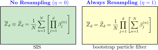
Figure 15: Expressions of the marginal likelihood estimators $\overline{Z}_{d}$ and $\widehat{Z}_{d}$ in two extreme scenarios: without resampling and applying resampling at each iterations. Note that in the formulations above the operations of sum and product are inverted.

Appendix D Particle Marginal Metropolis-Hastings (PMMH) algorithms

Let us consider ${\bf x}=x_{1:D}=[x_{1},x_{2},\ldots,x_{D}]\in\mathcal{X}\subseteq\mathbb{R}^{D\times\xi}$ where $x_{d}\in\mathbb{R}^{\xi}$ for all $d=1,\ldots,D$ and an additional model parameter ${\bm{\theta}}\in\mathbb{R}^{d_{\theta}}$ to be inferred as well. Assuming a prior pdf $g_{\theta}({\bm{\theta}})$ over ${\bm{\theta}}$, and a factorized complete posterior pdf $\bar{\pi}_{c}({\bf x},{\bm{\theta}})$

$$\bar{\pi}_{c}({\bf x},{\bm{\theta}})=\frac{g_{\theta}({\bm{\theta}})\pi({\bf x}|{\bm{\theta}})}{Z({\bm{\theta}})}\propto\pi_{c}({\bf x},{\bm{\theta}}) = g_{\theta}({\bm{\theta}})\pi({\bf x}|{\bm{\theta}}),$$ (93)

where $\pi({\bf x}|{\bm{\theta}})=\gamma_{1}(x_{1}|{\bm{\theta}})\prod_{d=2}^{D}\gamma_{d}(x_{d}|x_{1:d-1},{\bm{\theta}})$ and $Z({\bm{\theta}})=\int_{\mathbb{R}^{d_{\theta}}}g_{\theta}({\bm{\theta}})\pi({\bf x}|{\bm{\theta}})d{\bm{\theta}}$. Moreover, let us the denote as $\widehat{\pi}({\mathbf{x}}|{\mathbf{v}}_{1:N},{\bm{\theta}})=\frac{1}{N\widehat{Z}({\bm{\theta}})}\sum_{n=1}^{N}w({\mathbf{v}}_{n}|{\bm{\theta}})\delta({\mathbf{x}}-{\mathbf{v}}_{n})$ a particle approximation of $\pi({\bf x}|{\bm{\theta}})$ obtained by one run of a particle filter approach, and $\widehat{Z}({\bm{\theta}})=\frac{1}{N}\sum_{n=1}^{N}w({\mathbf{v}}_{n}|{\bm{\theta}})$ is an unbiased estimator of $Z({\bm{\theta}})$. The Marginal PMH (PMMH) technique is then summarized in Table 14. PMMH is often used for both smoothing and parameter estimation in state-space models. Note that if $q_{\theta}({\bm{\theta}}|{\bm{\theta}}_{t-1})=g_{\theta}({\bm{\theta}})$ then the acceptance function becomes

$$\alpha=\min\left[1,\frac{\widehat{Z}({\bm{\theta}}^{\prime})}{\widehat{Z}({\bm{\theta}}_{t-1})}\right].$$ (94)

Table 14: Particle Marginal MH (PMMH) algorithm

1. Choose ${\mathbf{x}}_{0}$, ${\bm{\theta}}_{0}$, and obtain a first estimation $\widehat{Z}({\bm{\theta}}_{0})$. 2. For $t=1,\ldots,T:$ (a) Draw ${\bm{\theta}}^{\prime}\sim q_{\theta}({\bm{\theta}}|{\bm{\theta}}_{t-1})$ and ${\mathbf{v}}_{j}\sim\widehat{\pi}({\mathbf{x}}|{\mathbf{v}}_{1:N},{\bm{\theta}}^{\prime})=\frac{1}{N\widehat{Z}({\bm{\theta}}^{\prime})}\sum_{n=1}^{N}w({\mathbf{v}}_{n}|{\bm{\theta}}^{\prime})\delta({\mathbf{x}}-{\mathbf{v}}_{n})$ (where $\widehat{\pi}$ is obtained with one run of a particle filter). (b) Set ${\bm{\theta}}_{t}={\bm{\theta}}^{\prime}$, ${\mathbf{x}}_{t}={\bf v}_{j}$, with probability $$\alpha=\min\left[1,\frac{\widehat{Z}({\bm{\theta}}^{\prime})g_{\theta}({\bm{\theta}}^{\prime})q_{\theta}({\bm{\theta}}_{t-1}|{\bm{\theta}}^{\prime})}{\widehat{Z}({\bm{\theta}}_{t-1})g_{\theta}({\bm{\theta}}_{t-1})q_{\theta}({\bm{\theta}}|{\bm{\theta}}_{t-1})}\right].$$ (95) Otherwise, set ${\bm{\theta}}_{t}={\bm{\theta}}^{\prime}$ and ${\mathbf{x}}_{t}={\mathbf{x}}_{t-1}$. 3. Return $\{{\mathbf{x}}_{t}\}_{t=1}^{T}$ and $\{{\bm{\theta}}_{t}\}_{t=1}^{T}$.

Distributed Particle Marginal Metropolis-Hastings (DPMMH).

We can easily design a marginal version of DPMH in Section 5.2, drawing ${\bm{\theta}}^{\prime}\sim q_{\theta}({\bm{\theta}}|{\bm{\theta}}_{t-1})$ and run $M$ particle filters addressing the target pdf ${\bar{\pi}}({\bf x}|{\bm{\theta}}^{\prime})$. The algorithm follows the steps in Table 14 with the difference that $M$ parallel particle filters are used, and in this case the acceptance probability is

$$\alpha=\min\left[1,\frac{\left[\sum_{m=1}^{M}\widehat{Z}_{m}({\bm{\theta}}^{\prime})\right]g_{\theta}({\bm{\theta}}^{\prime})q_{\theta}({\bm{\theta}}_{t-1}|{\bm{\theta}}^{\prime})}{\left[\sum_{m=1}^{M}\widehat{Z}_{m}({\bm{\theta}}_{t-1})\right]g_{\theta}({\bm{\theta}}_{t-1})q_{\theta}({\bm{\theta}}|{\bm{\theta}}_{t-1})}\right].$$ (96)

Appendix E GMS as infinite parallel IMTM2 chains

In this section, we show how the GMS can be interpreted as the use of infinite number of dependent parallel IMTM2 chains. We have already seen that we can recover an I-MTM2 chain from the GMS outputs applying one resampling step for each $t$ when $\mathcal{S}_{t}\neq\mathcal{S}_{t-1}$, i.e.,

$$\widetilde{{\bf x}}_{t}=\left\{\begin{split}&\widetilde{{\bf v}}_{t}\sim\sum_{n=1}^{N}\frac{\rho_{n,t}}{\sum_{i=1}^{N}\rho_{i,t}}\delta({\bf x}-{\bf x}_{n,t}),\quad\mbox{ if }\quad\mathcal{S}_{t}\neq\mathcal{S}_{t-1},\\ &\widetilde{{\bf x}}_{t-1},\quad\quad\quad\quad\quad\quad\quad\quad\quad\quad\mbox{ }\mbox{ if }\quad\mathcal{S}_{t}=\mathcal{S}_{t-1},\end{split}\right.$$ (97)

for $t=1,\ldots,T$. The sequence $\{\widetilde{{\bf x}}_{t}\}_{t=1}^{T}$ is a chain obtained by one run of an I-MTM2 technique. Note that (a )the sample generation, (b) the acceptance probability function and hence (c) the dynamics of GMS exactly coincide with the corresponding steps of I-MTM2 (or PMH; depending on candidate generation procedure). Hence, the ergodicity of the recovered chain is ensured.
Parallel chains from GMS outputs. We can extend the previous consideration for generation $C$ parallel I-MTM2 chains. Indeed, we resample independently $C$ times (instead of only one) within the set of accepted candidates at the $t$-th iteration $\{{\bf x}_{1,t},\ldots,{\bf x}_{N,t}\}$ , i.e.,

$$\widetilde{{\bf x}}_{t}^{(c)}=\left\{\begin{split}&\widetilde{{\bf v}}_{t}^{(c)}\sim\sum_{n=1}^{N}\frac{\rho_{n,t}}{\sum_{i=1}^{N}\rho_{i,t}}\delta({\bf x}-{\bf x}_{n,t}),\quad\mbox{ if }\quad\mathcal{S}_{t}\neq\mathcal{S}_{t-1},\\ &\widetilde{{\bf x}}_{t-1}^{(c)},\quad\quad\quad\quad\quad\quad\quad\quad\quad\quad\mbox{ }\mbox{ }\mbox{ }\mbox{ if }\quad\mathcal{S}_{t}=\mathcal{S}_{t-1},\end{split}\right.$$ (98)

for $c=1,\ldots,C$, where the super-index denotes the $c$-th chain (similar procedures have been suggested in [Calderhead, 2014, Martino et al., 2016b]). Clearly, the resulting $C$ parallel chains are not independent, and there is an evident loss in the performance w.r.t. the case of independent parallel chains (IPCs). However, at each iteration, the number of target evaluations per iteration is only $N$ instead of $NC$, as in the case of IPCs. Note that that each chain in ergodic, so that each estimator $\widetilde{I}_{T}^{(c)}=\frac{1}{T}\sum_{t=1}^{T}h(\widetilde{{\bf x}}_{t}^{(c)})$ is consistent for $T\rightarrow\infty$. As a consequence, the arithmetic mean of consistent estimators,

$$\widetilde{I}_{C,T}=\frac{1}{C}\sum_{c=1}^{C}\widetilde{I}_{T}^{(c)}=\frac{1}{CT}\sum_{t=1}^{T}\sum_{c=1}^{C}h(\widetilde{{\bf x}}_{t}^{(c)}),$$ (99)

is also consistent, for all values of $C\geq 1$.
GMS as limit case. Let us consider the case $\mathcal{S}_{t}\neq\mathcal{S}_{t-1}$ (the other is trivial), at some iteration $t$. In this scenario, the samples of the $C$ parallel I-MTM2 chains, $\widetilde{{\bf x}}_{t}^{(1)}$,$\widetilde{{\bf x}}_{t}^{(2)}$,…,$\widetilde{{\bf x}}_{t}^{(C)}$, are obtained by resampled independently $C$ samples from the set $\{{\bf x}_{1,t},\ldots,{\bf x}_{N,t}\}$ according to the normalized weights $\bar{\rho}_{n,t}=\frac{\rho_{n,t}}{\sum_{i=1}^{N}\rho_{i,t}}$, for $n=1,\ldots,N$. Recall that the samples $\widetilde{{\bf x}}_{t}^{(1)}$,$\widetilde{{\bf x}}_{t}^{(2)}$,…,$\widetilde{{\bf x}}_{t}^{(C)}$, will be used in the final estimator $\widetilde{I}_{C,T}$ in Eq. (99).

Let us denote as $\#j$ the number of times that a specific candidate ${\bf x}_{j,t}$ (contained in the set $\{{\bf x}_{n,t}\}_{n=1}^{N}$) has been selected as state of one of $C$ chains, at the $t$ iteration. As $C\rightarrow\infty$, The fraction $\frac{\#j}{C}$ approaches exactly the corresponding probability $\bar{\rho}_{j,t}$. Then, for $C\rightarrow\infty$, we have that the estimator in Eq. (99) approaches the GMS estimator, i.e.,

$$\widetilde{I}_{T}=\lim_{C\rightarrow\infty}\widetilde{I}_{C,T}=\frac{1}{T}\sum_{t=1}^{T}\sum_{n=1}^{N}\bar{\rho}_{n,t}h({\bf x}_{n,t}).$$ (100)

Since $\widetilde{I}_{C,T}$ as $T\rightarrow\infty$ is consistent for all values of $C$, then the GMS estimator $\widetilde{I}_{T}$ is also consistent (and can be obtained as $C\rightarrow\infty$).

References

- Liu [2004] J. S. Liu. Monte Carlo Strategies in Scientific Computing. Springer, 2004.
- Martino and Míguez [2009] L. Martino and J. Míguez. A novel rejection sampling scheme for posterior probability distributions. Proc. of the 34th IEEE ICASSP, April 2009.
- Martino et al. [2014a] L. Martino, J. Read, and D. Luengo. Independent doubly adaptive rejection Metropolis sampling. IEEE International Conference on Acoustics, Speech, and Signal Processing (ICASSP), pages 1–5, 2014a.
- Robert and Casella [2004] C. P. Robert and G. Casella. Monte Carlo Statistical Methods. Springer, 2004.
- Liang et al. [2010] F. Liang, C. Liu, and R. Caroll. Advanced Markov Chain Monte Carlo Methods: Learning from Past Samples. Wiley Series in Computational Statistics, England, 2010.
- Bugallo et al. [2015] M. F. Bugallo, L. Martino, and J. Corander. Adaptive importance sampling in signal processing. Digital Signal Processing, 47:36–49, 2015.
- Martino et al. [2017a] L. Martino, V. Elvira, D. Luengo, and J. Corander. Layered adaptive importance sampling. Statistics and Computing, 27(3):599–623, 2017a.
- Martino et al. [2015] L. Martino, V. Elvira, D. Luengo, and J. Corander. MCMC-driven adaptive multiple importance sampling. Interdisciplinary Bayesian Statistics Springer Proceedings in Mathematics & Statistics (Chapter 8), 118:97–109, 2015.
- Andrieu et al. [2003] C. Andrieu, N. de Freitas, A. Doucet, and M. Jordan. An introduction to MCMC for machine learning. Machine Learning, 50:5–43, 2003.
- Dangl et al. [2006] M. A. Dangl, Z. Shi, M. C. Reed, and J. Lindner. Advanced Markov chain Monte Carlo methods for iterative (turbo) multiuser detection. In Proc. 4th International Symposium on Turbo Codes and Related Topics in connection with 6th International ITG-Conference on Source and Channel Coding (ISTC), April 2006.
- Fitzgerald [2001] W. J. Fitzgerald. Markov chain Monte Carlo methods with applications to signal processing. Signal Processing, 81(1):3–18, January 2001.
- Martino [2018] L. Martino. A review of multiple try MCMC algorithms for signal processing. Digital Signal Processing, 75:134 – 152, 2018.
- Bugallo et al. [2017] M. F. Bugallo, V. Elvira, L. Martino, D. Luengo, J. Miguez, and P. M. Djuric. Adaptive importance sampling: The past, the present, and the future. IEEE Signal Processing Magazine, 34(4):60–79, 2017.
- Djurić et al. [2003] P. M. Djurić, J. H. Kotecha, J. Zhang, Y. Huang, T. Ghirmai, M. F. Bugallo, and J. Míguez. Particle filtering. IEEE Signal Processing Magazine, 20(5):19–38, September 2003.
- Elvira et al. [2015a] V. Elvira, L. Martino, D. Luengo, and M. F. Bugallo. Generalized multiple importance sampling. arXiv:1511.03095, 2015a.
- Candy [2009] J. Candy. Bayesian signal processing: classical, modern and particle filtering methods. John Wiley & Sons, England, 2009.
- Wang et al. [2002] X. Wang, R. Chen, and J. S. Liu. Monte Carlo Bayesian signal processing for wireless communications. Journal of VLSI Signal Processing, 30:89–105, 2002.
- Doucet and Wang [2005] A. Doucet and X. Wang. Monte Carlo methods for signal processing. IEEE Signal Processing Magazine, 22(6):152–170, Nov. 2005.
- Pereyra et al. [2016] M. Pereyra, P. Schniter, E. Chouzenoux, J. C. Pesquet, J. Y. Tourneret, A. Hero, and S. McLaughlin. A survey on stochastic simulation and optimization methods in signal processing. IEEE Sel. Topics in Signal Processing, 10(2):224–241, 2016.
- Ruanaidh and Fitzgerald [2012] J.J.K.O. Ruanaidh and W.J. Fitzgerald. Numerical Bayesian Methods Applied to Signal Processing. Springer, New York, 2012.
- Martino et al. [2017b] L. Martino, V. Elvira, and G. Camps-Valls. Group Metropolis Sampling. European Signal Processing Conference (EUSIPCO), pages 1–5, 2017b.
- Bolić et al. [2005] M. Bolić, P. M. Djurić, and S. Hong. Resampling algorithms and architectures for distributed particle filters. IEEE Transactions Signal Processing, 53(7):2442–2450, 2005.
- Míguez and Vázquez [2016] J. Míguez and M. A. Vázquez. A proof of uniform convergence over time for a distributed particle filter. Signal Processing, 122:152–163, 2016.
- Read et al. [2014] J. Read, K. Achutegui, and J. Míguez. A distributed particle filter for nonlinear tracking in wireless sensor networks. Signal Processing, 98:121 – 134, 2014.
- Verg et al. [2015] C. Verg , C. Dubarry, P. Del Moral, and E. Moulines. On parallel implementation of sequential Monte Carlo methods: the island particle model. Statistics and Computing, 25(2):243–260, 2015.
- Verg et al. [2014] C. Verg , P. Del Moral, E. Moulines, and J. Olsson. Convergence properties of weighted particle islands with application to the double bootstrap algorithm. arXiv:1410.4231, pages 1–39, 2014.
- Whiteley et al. [2016] N. Whiteley, A. Lee, and K. Heine. On the role of interaction in sequential Monte Carlo algorithms. Bernoulli, 22(1):494–529, 2016.
- Drovandi et al. [2014] C. C. Drovandi, J. McGree, and A. N. Pettitt. A sequential Monte Carlo algorithm to incorporate model uncertainty in Bayesian sequential design. Journal of Computational and Graphical Statistics, 23(1):3–24, 2014.
- Martino et al. [2017c] L. Martino, J. Read, V. Elvira, and F. Louzada. Cooperative parallel particle filters for on-line model selection and applications to urban mobility. Digital Signal Processing, 60:172–185, 2017c.
- Urteaga et al. [2016] I. Urteaga, M. F. Bugallo, and P. M. Djurić. Sequential Monte Carlo methods under model uncertainty. In 2016 IEEE Statistical Signal Processing Workshop (SSP), pages 1–5, 2016.
- Naesseth et al. [2015] C. A. Naesseth, F. Lindsten, and T. B. Schon. Nested Sequential Monte Carlo methods. Proceedings of theInternational Conference on Machine Learning, 37:1–10, 2015.
- Naesseth et al. [2016] C. A. Naesseth, F. Lindsten, and T. B. Schon. High-dimensional filtering using nested sequential Monte Carlo. arXiv:1612.09162, pages 1–48, 2016.
- Stern [2015] R. Bassi Stern. A statistical contribution to historical linguistics. Phd Thesis, 2015.
- Andrieu et al. [2010] C. Andrieu, A. Doucet, and R. Holenstein. Particle Markov chain Monte Carlo methods. J. R. Statist. Soc. B, 72(3):269–342, 2010.
- Bédard et al. [2012] M. Bédard, R. Douc, and E. Mouline. Scaling analysis of multiple-try MCMC methods. Stochastic Processes and their Applications, 122:758–786, 2012.
- Casarin et al. [2013] R. Casarin, R. V. Craiu, and F. Leisen. Interacting multiple try algorithms with different proposal distributions. Statistics and Computing, 23(2):185–200, 2013.
- Craiu and Lemieux [2007] R. V. Craiu and C. Lemieux. Acceleration of the Multiple Try Metropolis algorithm using antithetic and stratified sampling. Statistics and Computing, 17(2):109–120, 2007.
- Martino and Read [2013] L. Martino and J. Read. On the flexibility of the design of multiple try Metropolis schemes. Computational Statistics, 28(6):2797–2823, 2013.
- Martino and Louzada [2017] L. Martino and F. Louzada. Issues in the Multiple Try Metropolis mixing. Computational Statistics, 32(1):239–252, 2017.
- Casella and Robert [1996] G. Casella and C. P. Robert. Rao-Blackwellisation of sampling schemes. Biometrika, 83(1):81–94, 1996.
- Gamerman and Lopes [2006] D. Gamerman and H. F. Lopes. Markov Chain Monte Carlo: Stochastic Simulation for Bayesian Inference. Chapman & Hall/CRC Texts in Statistical Science, 2006.
- Brooks and Gelman [1998] S. P. Brooks and A. Gelman. General methods for monitoring convergence of iterative simulations. J. Comput. Graph. Statist., 7(4):434–455, 1998.
- Gelman and Rubin [1992] A. Gelman and D. B. Rubin. Inference from iterative simulation using multiple sequences. Statistical Science, 7(4):457–472, 1992.
- Propp and Wilson [1996] J. G. Propp and D. B. Wilson. Exact sampling with coupled Markov chains and applications to statistical mechanics. Random Structures Algorithms, 9:223–252, 1996.
- Wong and Liang [1997] W. H. Wong and F. Liang. Dynamic weighting in Monte Carlo and optimization. Proceedings of the National Academy of Sciences (PNAS), 94(26):14220–14224, 1997.
- Elvira et al. [2015b] V. Elvira, L. Martino, D. Luengo, and M. Bugallo. Efficient multiple importance sampling estimators. IEEE Signal Processing Letters, 22(10):1757–1761, 2015b.
- Elvira et al. [2016] V. Elvira, L. Martino, D. Luengo, and M. F. Bugallo. Heretical multiple importance sampling. IEEE Signal Processing Letters, 23(10):1474–1478, 2016.
- Martino et al. [2016a] L. Martino, V. Elvira, and F. Louzada. Weighting a resampled particle in Sequential Monte Carlo. IEEE Statistical Signal Processing Workshop, (SSP), 122:1–5, 2016a.
- Lamberti et al. [2016] R. Lamberti, Y. Petetin, F. Septier, and F. Desbouvries. An improved sir-based sequential Monte Carlo algorithm. In IEEE Statistical Signal Processing Workshop (SSP), pages 1–5, 2016.
- Doucet et al. [2001] A. Doucet, N. de Freitas, and N. Gordon, editors. Sequential Monte Carlo Methods in Practice. Springer, New York (USA), 2001.
- Huggins and Roy [2015] J. H Huggins and D. M Roy. Convergence of sequential Monte Carlo based sampling methods. arXiv:1503.00966, 2015.
- Martino et al. [2017d] L. Martino, V. Elvira, and M. F. Louzada. Effective Sample Size for importance sampling based on the discrepancy measures. Signal Processing, 131:386–401, 2017d.
- Doucet and Johansen [2008] A. Doucet and A. M. Johansen. A tutorial on particle filtering and smoothing: fifteen years later. technical report, 2008.
- Rubin [1988] D. B. Rubin. Using the SIR algorithm to simulate posterior distributions. in Bayesian Statistics 3, ads Bernardo, Degroot, Lindley, and Smith. Oxford University Press, Oxford, 1988., 1988.
- Martino et al. [2014b] L. Martino, F. Leisen, and J. Corander. On multiple try schemes and the Particle Metropolis-Hastings algorithm. viXra:1409.0051, 2014b.
- Martino et al. [2012] L. Martino, V. P. Del Olmo, and J. Read. A multi-point Metropolis scheme with generic weight functions. Statistics & Probability Letters, 82(7):1445–1453, 2012.
- Bishop [2006] C. Bishop. Pattern Recognition and Machine Learning. Springer, 2006.
- Rasmussen and Williams [2006] C. E. Rasmussen and C. K. I. Williams. Gaussian processes for machine learning. MIT Press, 2006.
- Haario et al. [2001] H. Haario, E. Saksman, and J. Tamminen. An adaptive Metropolis algorithm. Bernoulli, 7(2):223–242, April 2001.
- Ali et al. [2007] A. M. Ali, K. Yao, T. C. Collier, E. Taylor, D. Blumstein, and L. Girod. An empirical study of collaborative acoustic source localization. Proc. Information Processing in Sensor Networks (IPSN07), Boston, April 2007.
- Ihler et al. [2005] A. T. Ihler, J. W. Fisher, R. L. Moses, and A. S. Willsky. Nonparametric belief propagation for self-localization of sensor networks. IEEE Transactions on Selected Areas in Communications, 23(4):809–819, April 2005.
- Cornuet et al. [2012] J. M. Cornuet, J. M. Marin, A. Mira, and C. P. Robert. Adaptive multiple importance sampling. Scandinavian Journal of Statistics, 39(4):798–812, December 2012.
- Patwari et al. [2003] N. Patwari, A. O. Hero, M. Perkins, N. S. Correal, and R. J. O’Dea. Relative location estimation in wireless sensor networks. IEEE Transactions Signal Processing, 51(5):2137–2148, 2003.
- Rappaport [2001] T. S. Rappaport. Wireless Communications: Principles and Practice (2nd edition). Prentice-Hall, Upper Saddle River, NJ (USA), 2001.
- Chen and Black [1992] J. M. Chen and T. A Black. Defining leaf area index for non-flat leaves. Plant, Cell and Environment, 15:421–429, 1992.
- Gomez-Dans et al. [2016] J. L. Gomez-Dans, P. E. Lewis, and M. Disney. Efficient emulation of radiative transfer codes using Gaussian Processes and application to land surface parameter inferences. Remote Sensing, 8(2), 2016.
- Calderhead [2014] B. Calderhead. A general construction for parallelizing Metropolis-Hastings algorithms. Proceedings of the National Academy of Sciences of the United States of America (PNAS), 111(49):17408–17413, 2014.
- Martino et al. [2016b] L. Martino, V. Elvira, D. Luengo, J. Corander, and F. Louzada. Orthogonal parallel MCMC methods for sampling and optimization. Digital Signal Processing, 58:64–84, 2016b.