A branched transport limit of the Ginzburg-Landau functional

Abstract

We study the Ginzburg-Landau model of type-I superconductors in the regime of small external magnetic fields. We show that, in an appropriate asymptotic regime, flux patterns are described by a simplified branched transportation functional. We derive the simplified functional from the full Ginzburg-Landau model rigorously via $\Gamma$-convergence. The detailed analysis of the limiting procedure and the study of the limiting functional lead to a precise understanding of the multiple scales contained in the model.

1 Introduction

In 1911, K. Onnes discovered the phenomenon of superconductivity, manifested in the complete loss of resistivity of certain metals and alloys at very low temperature. W. Meissner discovered in 1933 that this was coupled with the expulsion of the magnetic field from the superconductor at the critical temperature. This is now called the Meissner effect. After some preliminary works of the brothers F. and H. London, V. Ginzburg and L. Landau proposed in 1950 a phenomenological model describing the state of a superconductor. In their model (see (1.1) below), which belongs to Landau’s general theory of second-order phase transitions, the state of the material is represented by the order parameter $u:\Omega\to\mathbb{C}$, where $\Omega$ is the material sample. The density of superconducting electrons is then given by $\rho:=|u|^{2}$. A microscopic theory of superconductivity was first proposed by Bardeen-Cooper-Schrieffer (BCS) in 1957, and the Ginzburg-Landau model was derived from BCS by Gorkov in 1959 (see also [FHSS12] for a rigorous derivation).

One of the main achievements of the Ginzburg-Landau theory is the prediction and the understanding of the mixed (or intermediate) state below the critical temperature. This is a state in which, for moderate external magnetic fields, normal and superconducting regions coexist. The behavior of the material in the Ginzburg-Landau theory is characterized by two physical parameters. The first is the coherence length $\xi$ which measures the typical length on which $u$ varies, the second is the penetration length $\lambda$ which gives the typical length on which the magnetic field penetrates the superconducting regions. The Ginzburg-Landau parameter is then defined as $\kappa:=\frac{\lambda}{\xi}$. The Ginzburg-Landau functional is given by

$$\int_{\Omega}|\nabla_{A}u|^{2}+\frac{\kappa^{2}}{2}(1-|u|^{2})^{2}dx+\int_{\mathbb{R}^{3}}|\nabla\times A-B_{\mathrm{ext}}|^{2}dx$$ (1.1)

where $A:\mathbb{R}^{3}\to\mathbb{R}^{3}$ is the magnetic potential (so that $B:=\nabla\times A$ is the magnetic field), $\nabla_{A}u:=\nabla u-iAu$ is the covariant derivative of $u$ and $B_{\mathrm{ext}}$ is the external magnetic field. In these units, the penetration length $\lambda$ is normalized to $1$. As first observed by A. Abrikosov this theory predicts two types of superconductors. On the one hand, when $\kappa<1/\sqrt{2}$, there is a positive surface tension which leads to the formation of normal and superconducting regions corresponding to $\rho\simeq 0$ and $\rho\simeq 1$ respectively, separated by interfaces. These are the so-called type-I superconductors. On the other hand, when $\kappa>1/\sqrt{2}$, this surface tension is negative and one expects to see the magnetic field penetrating the domain through lines of vortices. These are the so-called type-II superconductors. In this paper we are interested in better understanding the former type but we refer the interested reader to [Tin96, SS07, Ser15] for more information about the latter type. In particular, in that regime, there has been an intensive work on understanding the formation of regular patterns of vortices known as Abrikosov lattices.

In type-I superconductors, it is observed experimentally [PH09, Pro07, PGPP05] that complex patterns appear at the surface of the sample. It is believed that these patterns are a manifestation of branching patterns inside the sample. Although the observed states are highly history-dependent, it is argued in [CKO04, PGPP05] that the hysteresis is governed by low-energy configurations at vanishing external magnetic field. The scaling law of the ground-state energy was determined in [CCKO08, CKO04] for a simplified sharp interface version of the Ginzburg-Landau functional (1.1) and in [COS16] for the full energy, these results indicate the presence of a regime with branched patterns at low fields.

This paper aims at a better understanding of these branched patterns by going beyond the scaling law. Starting from the full Ginzburg-Landau functional, we prove that in the regime of vanishing external magnetic field, low energy configurations are made of nearly one-dimensional superconducting threads branching towards the boundary of the sample. In a more mathematical language, we prove $\Gamma-$convergence [Bra02, DM93] of the Ginzburg-Landau functional to a kind of branched transportation functional in this regime. We focus on the simplest geometric setting by considering the sample $\Omega$ to be a box $Q_{L_{0},T}:=(-\frac{L_{0}}{2},\frac{L_{0}}{2})^{2}\times(-T,T)$ for some $T,L_{0}>0$ and consider periodic lateral boundary conditions. The external magnetic field is taken to be perpendicular to the sample, that is $B_{\mathrm{ext}}:=b_{\mathrm{ext}}e_{3}$ for some $b_{\mathrm{ext}}>0$ and where $e_{3}$ is the third vector of the canonical basis of $\mathbb{R}^{3}$. After making an isotropic rescaling, subtracting the bulk part of the energy and dropping lower order terms (see (3.5) and the discussion after it), minimizing (1.1) can be seen as equivalent to minimizing

$$E_{T}(u,A):=\frac{1}{L^{2}}\int_{Q_{L,1}}|\nabla_{TA}u|^{2}+\left(B_{3}-\alpha(1-\rho)\right)^{2}+|B^{\prime}|^{2}dx+\|B_{3}-\alpha\beta\|_{H^{-1/2}(\{x_{3}=\pm 1\})}^{2},\,$$ (1.2)

where we have let $B:=(B^{\prime},B_{3}):=\nabla\times A$,

$$\kappa T:=\sqrt{2}\alpha,\qquad b_{\mathrm{ext}}:=\frac{\beta\kappa}{\sqrt{2}}\qquad\textrm{ and }\qquad L:=L_{0}/T.$$

If $u=\rho^{1/2}\exp(i\theta)$, since $|\nabla_{TA}u|^{2}=|\nabla\rho^{1/2}|^{2}+\rho|\nabla\theta-TA|^{2}$, in the limit $T\to+\infty$ we obtain, at least formally, that $A$ is a gradient field in the region where $\rho>0$ and therefore the Meissner condition $\rho B=0$ holds. Moreover, in the regime $\alpha\gg 1$, from (1.2) we see that $B_{3}\simeq\alpha(1-\rho)$ and $\rho$ takes almost only values in $\{0,1\}$. Hence $\textup{div}\,B=0$ can be rewritten as

$$\partial_{3}\chi+\frac{1}{\alpha}\textup{div}\,\!^{\prime}\chi B^{\prime}=0,$$

where $\chi:=(1-\rho)$ and $\textup{div}\,\!^{\prime}$ denotes the divergence with respect to the first two variables. Therefore, from the Benamou-Brenier formulation of optimal transportation [AGS05, Vil03] and since from the Meissner condition, $B^{\prime}\simeq\frac{1}{\chi}B^{\prime}$, the term

$$\int_{Q_{L,1}}|B^{\prime}|^{2}dx\simeq\int_{Q_{L,1}}\frac{1}{\chi}|B^{\prime}|^{2}dx$$

in the energy (1.2) can be seen as a transportation cost. We thus expect that inside the sample (this is, in $Q_{L,1}$), superconducting domains where $\rho\simeq 1$ and $B\simeq 0$ alternate with normal ones where $\rho\simeq 0$ and $B_{3}\simeq\alpha$. Because of the last term $\|B_{3}-\alpha\beta\|_{H^{-1/2}(\{x_{3}=\pm 1\})}^{2}$ in the energy (1.2), one expects $B\simeq\alpha\beta e_{3}$ outside the sample. This implies that close to the boundary the normal domains have to refine. The interaction between the surface energy, the transportation cost and the penalization of an $H^{-1/2}$ norm leads to the formation of complex patterns (see Figure 1).

It has been proven in [COS16] that in the regime $T\gg 1$, $\alpha\gg 1$ and $\beta\ll 1$,

$$\min E_{T}(u,A)\sim\min\{\alpha^{4/3}\beta^{2/3},\alpha^{10/7}\beta\}\,.$$ (1.3)

The scaling $\min E_{T}(u,A)\sim\alpha^{4/3}\beta^{2/3}$ (relevant for $\alpha^{-2/7}\ll\beta$) corresponds to uniform branching patterns whereas the scaling $\min E_{T}(u,A)\sim\alpha^{10/7}\beta$ corresponds to non-uniform branching ones. We focus here for definiteness on the regime $\min E_{T}(u,A)\sim\alpha^{4/3}\beta^{2/3}$, although we believe that our proof can be extended to the other one. Based on the construction giving the upper bounds in (1.3), we expect that in the first regime there are multiple scales appearing (see Figure 1):

$$\stackrel{{\scriptstyle\displaystyle\textrm{penetration}}}{{\textrm{ length}}}\,\stackrel{{\scriptstyle\displaystyle\ll}}{{\,}}\,\stackrel{{\scriptstyle\displaystyle\textrm{ coherence}}}{{\textrm{ length}}}\,\stackrel{{\scriptstyle\displaystyle\ll}}{{\,}}\,\stackrel{{\scriptstyle\displaystyle\textrm{ diameter of the}}}{{\textrm{ threads in the bulk}}}\,\,\stackrel{{\scriptstyle\displaystyle\ll}}{{\,}}\,\,\stackrel{{\scriptstyle\displaystyle\textrm{distance between the}}}{{\textrm{ threads in the bulk}}},$$ (1.4)

which amounts in our parameters to

$$T^{-1}\ll\alpha^{-1}\ll\alpha^{-1/3}\beta^{1/3}\ll\alpha^{-1/3}\beta^{-1/6}.$$

Figure 1: The various lengthscales

In order to better describe the minimizers we focus on the extreme region of the phase diagram $T,T\alpha^{-1},\beta^{-1},\alpha\beta^{7/2}\to+\infty$, with $L=\widetilde{L}\alpha^{-1/3}\beta^{-1/6}$ for some fixed $\widetilde{L}>0$. In this regime, we have in particular $\alpha^{-1}\ll\alpha^{-1/3}\beta^{1/3}$ so that the separation of scales (1.4) holds. We introduce an anisotropic rescaling (see Section 3) which leads to the functional

$$\widetilde{E}_{T}(u,A) :=\frac{1}{\widetilde{L}^{2}}\Big{[}\int_{Q_{\widetilde{L},1}}\alpha^{-2/3}\beta^{-1/3}\left|\nabla_{\alpha^{1/3}\beta^{-1/3}TA}^{\prime}u\right|^{2}+\alpha^{-4/3}\beta^{-2/3}\left|(\nabla_{\alpha^{1/3}\beta^{-1/3}TA}u)_{3}\right|^{2}$$ (1.5)

$$+ \left.\alpha^{2/3}\beta^{-2/3}\left({B_{3}}-(1-|{u}|^{2})\right)^{2}+\beta^{-1}|{B^{\prime}}|^{2}dx+\alpha^{1/3}\beta^{7/6}\|\beta^{-1}{B_{3}}-1\|_{H^{-1/2}(x_{3}=\pm 1)}^{2}\right].$$

Our main result is a $\Gamma-$convergence result of the functional $\widetilde{E}_{T}$ towards a functional defined on measures $\mu$ living on one-dimensional trees. These trees correspond to the normal regions in which $\rho\simeq 0$ and where the magnetic field $B$ penetrates the sample. Roughly speaking, if for a.e. $x_{3}\in(-1,1)$ the slice of $\mu=\mu_{x_{3}}\otimes dx_{3}$ has the form $\mu_{x_{3}}=\sum_{i}\varphi_{i}\delta_{X_{i}(x_{3})}$ where the sum is at most countable, then we let (see Section 5 for a precise definition)

$$I(\mu):=\frac{1}{\widetilde{L}^{2}}\int_{-1}^{1}K_{*}\sum_{i}\sqrt{\varphi_{i}}+\varphi_{i}|\dot{X}_{i}|^{2}dx_{3},$$ (1.6)

where $K_{*}=8\sqrt{\pi}/3$ and $\dot{X}_{i}$ denotes the derivative (with respect to $x_{3}$) of $X_{i}(x_{3})$. The $X_{i}$’s represent the graphs of each branch of the tree (parametrized by height) and the $\varphi_{i}$’s represent the flux carried by the branch. We can now state our main result

Theorem 1.1.

Let $T_{n},\alpha_{n},\beta_{n}^{-1}\to+\infty$ with $T_{n}\alpha_{n}^{-1},\alpha_{n}\beta_{n}^{7/2}\to+\infty$, $\widetilde{L}>0$, then:

1. For every sequence $(u_{n},A_{n})$ with $\sup_{n}\widetilde{E}_{T}(u_{n},A_{n})<+\infty$, up to subsequence , $\beta_{n}^{-1}(1-|u_{n}|^{2})$ weakly converges to a measure $\mu$ of the form $\mu=\mu_{x_{3}}\otimes dx_{3}$ with $\mu_{x_{3}}=\sum_{i}\varphi_{i}\delta_{X_{i}}$ for a.e. $x_{3}\in(-1,1)$, $\mu_{x_{3}}\rightharpoonup dx^{\prime}$ (where $dx^{\prime}$ denotes the two dimensional Lebesgue measure on $Q_{\widetilde{L}}$) when $x_{3}\to\pm 1$ and such that

   $$\liminf_{n\to+\infty}\widetilde{E}_{T}(u_{n},A_{n})\geq I(\mu).$$

2. If in addition $L_{n}^{2}\alpha_{n}\beta_{n}T_{n}\in 2\pi\mathbb{Z}$, where $L_{n}:=\widetilde{L}\alpha_{n}^{-1/3}\beta_{n}^{-1/6}$, then for every measure $\mu$ such that $I(\mu)<+\infty$ and $\mu_{x_{3}}\rightharpoonup dx^{\prime}$ as $x_{3}\to\pm 1$ , there exists $(u_{n},A_{n})$ such that $\beta_{n}^{-1}(1-|u_{n}|^{2})\rightharpoonup\mu$ and

   $$\limsup_{n\to+\infty}\,\widetilde{E}_{T}(u_{n},A_{n})\leq I(\mu).$$

Proof.

By scaling, it suffices to consider the case $\widetilde{L}=1$. The first assertion follows from Proposition 6.1, the second one from Proposition 7.1. ∎

Let us stress once again that our result could have been equivalently stated for the full Ginzburg-Landau energy (1.1) instead of $\widetilde{E}_{T}$ (see Section 3).
Within our periodic setting, the quantization condition $L_{n}^{2}\alpha_{n}\beta_{n}T_{n}\in 2\pi\mathbb{Z}$ for the flux is a consequence of the fact that the phase circulation of the complex-valued function in the original problem is naturally quantized. It is necessary in order to make our construction but we believe that it is also a necessary condition for having sequences of bounded energy (see the discussion in Section 3 and the construction in Section 7.3). We remark that scaling back to the original variables this condition is the physically natural one $L_{0}^{2}b_{\mathrm{ext}}\in 2\pi\mathbb{Z}$.

Before going into the proof of Theorem 1.1 we address the limiting functional $I(\mu)$, which has many similarities with irrigation (or branched transportation) models that have recently attracted a lot of attention (see [BCM09] and more detailed comments in Section 5.4 or the recent papers [BW15, BRW16] where the connection is also made to some urban planning models). In Section 5, we first prove that the variational problem for this limiting functional is well-posed (Proposition 5.5) and show a scaling law for it (Proposition 5.2 and Proposition 5.3). In Proposition 5.7, we define the notion of subsystems which allows us to remove part of the mass carried by the branching measure. This notion is at the basis of Lemma 5.8 and Proposition 5.11 which show that minimizers contain no loops and that far from the boundary, they are made of a finite number of branches. From the no-loop property, we easily deduce Proposition 5.10 which is a regularity result for minimizers of $I$. The main result of Section 5 is Theorem 5.15 which proves the density of “regular” measures in the topology given by the energy $I(\mu)$. As in nearly every $\Gamma-$convergence result, such a property is crucial in order to implement the construction for the upper bound (ii).

We now comment on the proof of Theorem 1.1. Let us first point out that if the Meissner condition $\rho B=0$ were to hold, and $A$ could be written as a gradient field in the set $\{\rho>0\}$, then $|\nabla_{TA}u|^{2}=|\nabla\rho^{1/2}|^{2}$ and we would have

$$\int_{Q_{L,1}}|\nabla_{TA}u|^{2}+\left(B_{3}-\alpha(1-\rho)\right)^{2}dx=\int_{Q_{L,1}}|\nabla\rho^{1/2}|^{2}+\alpha^{2}\chi_{\rho>0}(1-\rho)^{2}+\chi_{\rho=0}(B_{3}-\alpha)^{2}dx.$$ (1.7)

This is a Modica-Mortola [Mod87] type of functional with a degenerate double-well potential given by $W(\rho):=\chi_{\rho>0}(1-\rho)^{2}$. Thanks to Lemma 6.2, one can control how far we are from satisfying the Meissner condition. From this, we deduce that (1.7) almost holds (see Lemma 6.5). This implies that the Ginzburg-Landau energy gives a control over the perimeter of the superconducting region $\{\rho>0\}$. In addition, $\beta\ll 1$ imposes a small cross-area fraction for $\{\rho>0\}$. Using then isoperimetric effects to get convergence to one-dimensional objects (see Lemma 6.6), we may use Proposition 6.1 to conclude the proof of (i).

In order to prove (ii), thanks to the density result in Theorem 5.15, it is enough to consider regular measures. Given such a measure $\mu$, we first approximate it with quantized measures (Lemma 5.18). Far from branching points the construction is easy (see Lemma 7.3). At a branching point, we need to pass from one disk to two (or vice-versa); this is done passing through rectangles (see Lemma 7.6 and Figure 3). Close to the boundary we use instead the construction from [COS16], which explicitly generates a specific branching pattern with the optimal energy scaling; since the height over which this is done is small the prefactor is not relevant here (Proposition 7.7). The last step is to define a phase and a magnetic potential to get back to the full Ginzburg-Landau functional. This is possible since we made the construction with the Meissner condition and quantized fluxes enforced, see Proposition 7.8.

From (1.2) and the discussion around (1.7), for type-I superconductors, the Ginzburg-Landau functional can be seen as a non-convex, non-local (in $u$) functional favoring oscillations, regularized by a surface term which selects the lengthscales of the microstructures. The appearance of branched structures for this type of problem is shared by many other functionals appearing in material sciences such as shape memory alloys [KM92, KM94, Con00, KKO13, BG15, Zwi14, CC15, CZ16], uniaxial ferromagnets [CKO99, OV10, KM11] and blistered thin films [BCDM00, JS01, BCDM02]. Most of the previously cited results on branching patterns (including [CCKO08, CKO04, COS16] for type-I superconductors) focus on scaling laws. Here, as in [OV10, CDZ17], we go one step further and prove that, after a suitable anisotropic rescaling, configurations of low energy converge to branched patterns. The two main difficulties in our model with respect to the one studied in [OV10] are the presence of an additional lengthscale (the penetration length) and its sharp limit counterpart, the Meissner condition $\rho B=0$ which gives a nonlinear coupling between $u$ and $B$. Let us point out that for the Kohn-Müller model [KM92, KM94], a much stronger result is known, namely that minimizers are asymptotically self-similar [Con00] (see also [Vie09, ACO09] for related results). In [Gol17], the optimal microstructures for a two-dimensional analogue of $I(\mu)$ are exactly computed.

The paper is organized as follows. In section 2, we set some notation and recall some notions from optimal transport theory. In Section 3, we recall the definition of the Ginzburg-Landau functional together with various important quantities such as the superconducting current. We also introduce there the anisotropic rescaling leading to the functional $\widetilde{E}_{T}$. In Section 4, we introduce for the sake of clarity intermediate functionals corresponding to the different scales of the problem. Let us stress that we will not use them in the rest of the paper but strongly believe that they help understanding the structure of the problem. In Section 5, we carefuly define the limiting functional $I(\mu)$ and study its properties. In particular we recover a scaling law for the minimization problem and prove regularity of the minimizers. We then prove the density in energy of ’regular’ measures. This is a crucial result for the main $\Gamma-$ convergence result which is proven in the last two sections. As customary, we first prove the lower bound in Section 6 and then make the upper bound construction in Section 7.

2 Notation and preliminary results

In the paper we will use the following notation. The symbols $\sim$, $\gtrsim$, $\lesssim$ indicate estimates that hold up to a global constant. For instance, $f\lesssim g$ denotes the existence of a constant $C>0$ such that $f\leq Cg$, $f\sim g$ means $f\lesssim g$ and $g\lesssim f$. In heuristic arguments we use $a\simeq b$ to indicate that $a$ is close (in a not precisely specified sense) to $b$. We use a prime to indicate the first two components of a vector in $\mathbb{R}^{3}$, and identify $\mathbb{R}^{2}$ with $\mathbb{R}^{2}\times\{0\}\subseteq\mathbb{R}^{3}$. Precisely, for $a\in\mathbb{R}^{3}$ we write $a^{\prime}=(a_{1},a_{2},0)\in\mathbb{R}^{2}\subseteq\mathbb{R}^{3}$; given two vectors $a,b\in\mathbb{R}^{3}$ we write $a^{\prime}\times b^{\prime}=(a\times b)_{3}=(a^{\prime}\times b^{\prime})_{3}$. We denote by $(e_{1},e_{2},e_{3})$ the canonical basis of $\mathbb{R}^{3}$. For $L>0$ and $T>0$, $Q_{L}:=(-\frac{L}{2},\frac{L}{2})^{2}$ and $Q_{L,T}:=Q_{L}\times(-T,T)$. For a function $f$ defined on $Q_{L,T}$, we denote $f_{x_{3}}$ the function $f_{x_{3}}(x^{\prime}):=f(x^{\prime},x_{3})$ and we analogously define for $\Omega\subseteq Q_{L,T}$, the set $\Omega_{x_{3}}$. For $x=(x^{\prime},x_{3})$ and $r>0$ we let $\mathcal{B}_{r}(x)=\mathcal{B}(x,r)$ be the ball of radius $r$ centered at $x$ (in $\mathbb{R}^{3}$) and $\mathcal{B}^{\prime}_{r}(x^{\prime})=\mathcal{B}^{\prime}(x^{\prime},r)$ be the analogue two-dimensional ball centered at $x^{\prime}$. Unless specified otherwise, all the functions and measures we will consider are periodic in the $x^{\prime}$ variable, i.e., we identify $Q_{L}$ with the torus $\mathbb{R}^{2}/L\mathbb{Z}^{2}$. In particular, for $x^{\prime},y^{\prime}\in Q_{L}$, $|x^{\prime}-y^{\prime}|$ denotes the distance for the metric of the torus, i.e., $|x^{\prime}-y^{\prime}|:=\min_{k\in\mathbb{Z}^{2}}|x^{\prime}-y^{\prime}+Lk|$. We denote by $\mathcal{H}^{k}$ the $k-$dimensional Hausdorff measure. We let $\mathcal{P}(Q_{L})$ be the space of probability measures on $Q_{L}$ and $\mathcal{M}(Q_{L,T})$ be the space of finite Radon measures on $Q_{L,T}$, and similarly $\mathcal{M}(Q_{L})$. Analogously, we define $\mathcal{M}^{+}(Q_{L,T})$ and $\mathcal{M}^{+}(Q_{L})$ as the spaces of finite Radon measures which are also positive. For a measure $\mu$ and a function $f$, we denote by $f\sharp\mu$ the push-forward of $\mu$ by $f$.

We recall the definition of the (homogeneous) $H^{-1/2}$ norm of a function $f\in L^{2}(Q_{L})$ with $\int_{Q_{L}}fdx^{\prime}=0$,

$$\|f\|_{H^{-1/2}}^{2}:=\inf\left\{\int_{Q_{L}\times[0,+\infty)}|B|^{2}dx\ :\ \textup{div}\,B=0,\ B_{3}(\cdot,0)=f\right\},$$ (2.1)

which can be alternatively given in term of the two-dimensional Fourier series as (see, e.g., [CKO04])

$$\|f\|_{H^{-1/2}}^{2}=\frac{1}{2\pi}\sum_{k^{\prime}\in\left(\frac{2\pi}{L}\mathbb{Z}\right)^{2}\backslash\{0\}}\frac{|\hat{f}(k^{\prime})|^{2}}{|k^{\prime}|}.$$

We shall write $\|f\|^{2}_{H^{-1/2}(Q_{L}\times\{\pm T\})}$ for $\|f\|^{2}_{H^{-1/2}(Q_{L}\times\{T\})}+\|f\|^{2}_{H^{-1/2}(Q_{L}\times\{-T\})}$.

The $2$-Wasserstein distance between two measures $\mu$ and $\nu\in\mathcal{M}^{+}(Q_{L})$ with $\mu(Q_{L})=\nu(Q_{L})$ is given by

$$W_{2}^{2}(\mu,\nu):=\min\left\{\mu(Q_{L})\int_{Q_{L}\times Q_{L}}|x-y|^{2}\,d\Pi(x,y)\,:\,\Pi_{1}=\mu,\ \Pi_{2}=\nu\right\},$$

where the minimum is taken over measures on $Q_{L}\times Q_{L}$ and $\Pi_{1}$ and $\Pi_{2}$ are the first and second marginal of $\Pi$, respectively. For measures $\mu,\nu\in\mathcal{M}^{+}(Q_{L,T})$, the $2$-Wasserstein distance is correspondingly defined. We now introduce some notions from metric analysis, see [AGS05, Vil03] for more detail. A curve $\mu:(a,b)\to\mathcal{P}(Q_{L})$, $z\mapsto\mu_{z}$ belongs to $AC^{2}(a,b)$ (where $AC$ stands for absolutely continuous) if there exists $m\in L^{2}(a,b)$ such that

$$W_{2}(\mu_{z},\mu_{\widetilde{z}})\leq\int_{z}^{\widetilde{z}}m(t)dt\ \qquad\forall a<z\leq\widetilde{z}<b.$$ (2.2)

For any such curve, the speed

$$|\mu^{\prime}|(z):=\lim_{\widetilde{z}\to z}\frac{W_{2}(\mu_{\widetilde{z}},\mu_{z})}{|z-\widetilde{z}|}$$

exists for $\mathcal{H}^{1}-$a.e. $z\in(a,b)$ and $|\mu^{\prime}|(z)\leq m(z)$ for $\mathcal{H}^{1}$-a.e. $z\in(a,b)$ for every admissible $m$ in (2.2). Further, there exists a Borel vector field $B$ such that

$$B(\cdot,z)\in L^{2}(Q_{L},\mu_{z}),\qquad\|B(\cdot,z)\|_{L^{2}(Q_{L},\mu_{z})}\leq|\mu^{\prime}|(z)\quad\textrm{for }\mathcal{H}^{1}\text{-a.e. }\ z\in(a,b)$$ (2.3)

and the continuity equation

$$\partial_{3}\mu_{z}+\textup{div}\,\!^{\prime}(B\mu_{z})=0$$ (2.4)

holds in the sense of distributions [AGS05, Th. 8.3.1]. Conversely, if a weakly continuous curve $\mu_{z}:(a,b)\to\mathcal{P}(Q_{L})$ satisfies the continuity equation (2.4) for some Borel vector field $B$ with $\|B(\cdot,z)\|_{L^{2}(Q_{L},\mu_{z})}\in L^{2}(a,b)$ then $\mu\in AC^{2}(a,b)$ and $|\mu^{\prime}|(z)\leq\|B(\cdot,z)\|_{L^{2}(Q_{L},\mu_{z})}$ for $\mathcal{H}^{1}$-a.e. $z\in(a,b)$. In particular, we have

$$W_{2}^{2}(\nu,\hat{\nu})=\min_{\mu,B}\left\{2T\int_{Q_{L,T}}|B|^{2}d\mu_{z}dz\ :\ \mu_{-T}=\nu,\ \mu_{T}=\hat{\nu}\textrm{ and \eqref{conteqini} holds}\right\}\,,$$ (2.5)

where by scaling the right-hand side does not depend on $T$.

For a (signed) measure $\mu\in\mathcal{M}(Q_{L})$, we define the Bounded-Lipschitz norm of $\mu$ as

$$\|\mu\|_{BL}:=\sup_{\|\psi\|_{Lip}\leq 1}\int_{Q_{L}}\psi d\mu,$$ (2.6)

where for a $Q_{L}-$periodic and Lipschitz continuous function $\psi$, $\|\psi\|_{Lip}:=\|\psi\|_{\infty}+\|\nabla\psi\|_{\infty}$. By the Kantorovich-Rubinstein Theorem [Vil03, Th. 1.14], the $1-$Wasserstein and the Bounded-Lipschitz norm are equivalent.

3 The Ginzburg-Landau functional

In this section we recall some background material concerning the Ginzburg-Landau functional and introduce the anisotropic rescaling leading to $\widetilde{E}_{T}$.
For a (non necessarily periodic) function $u:Q_{L_{0},T}\to\mathbb{C}$, called the order parameter, and a vector potential $A:Q_{L_{0}}\times\mathbb{R}\to\mathbb{R}^{3}$ (also not necessarily periodic), we define the covariant derivative

$$\nabla_{A}u:=\nabla u-iAu,$$

the magnetic field

$$B:=\nabla\times A,$$

and the superconducting current

$$j_{A}:=\frac{1}{2}\left(-i\bar{u}(\nabla_{A}u)+iu(\overline{\nabla_{A}u})\right)=\textrm{Im}(iu\overline{\nabla_{A}u})\,.$$ (3.1)

Let us first notice that $|\nabla_{A}u|^{2}$ and the observable quantities $\rho$, $B$ and $j_{A}$ are invariant under change of gauge. That is, if we replace $u$ by $ue^{i\varphi}$ and $A$ by $A+\nabla\varphi$ for any function $\varphi$, they remain unchanged. We also point out that if $u$ is written in polar coordinates as $u=\rho^{1/2}e^{i\theta}$, then

$$|\nabla_{A}u|^{2}=|\nabla\rho^{1/2}|^{2}+\rho|\nabla\theta-A|^{2}.$$

For any admissible pair $(u,A)$, that is such that $\rho$, $B$ and $j_{A}$ are $Q_{L_{0}}$-periodic, we define the Ginzburg-Landau functional as

$$E_{\mathrm{GL}}(u,A):=\int_{Q_{L_{0},T}}|\nabla_{A}u|^{2}+\frac{\kappa^{2}}{2}(1-|u|^{2})^{2}dx+\int_{Q_{L_{0}}\times\mathbb{R}}|\nabla\times A-B_{\mathrm{ext}}|^{2}dx\,.$$

We remark that $u$ and $A$ need not be (and, if $B_{\mathrm{ext}}\neq 0$, cannot be) periodic. See [COS16] for more details on the functional spaces we are using. Here $B_{\mathrm{ext}}:=b_{\mathrm{ext}}e_{3}$ is the external magnetic field and $\kappa\in(0,1/\sqrt{2})$ is a material constant, called the Ginzburg-Landau parameter. From periodicity and $\textup{div}\,B=0$ it follows that $\int_{Q_{L_{0}}\times\{x_{3}\}}B_{3}\,dx^{\prime}$ does not depend on $x_{3}$ and therefore, if the energy is finite, necessarily

$$\int_{Q_{L_{0}}\times\{x_{3}\}}B_{3}\,dx^{\prime}=L_{0}^{2}b_{\mathrm{ext}}\hskip 28.45274pt\text{ for all }x_{3}\in\mathbb{R}\,.$$ (3.2)

We first remove the bulk part from the energy $E_{\mathrm{GL}}$. In order to do so, we introduce the quantity

$$\mathcal{D}_{A}^{3}u:=(\partial_{2}u-iA_{2}u)-i(\partial_{1}u-iA_{1}u)=(\nabla_{A}u)_{2}-i(\nabla_{A}u)_{1}$$

and, more generally,

$$\mathcal{D}_{A}^{k}u:=(\partial_{k+2}u-iA_{k+2}u)-i(\partial_{k+1}u-iA_{k+1}u)=(\nabla_{A}u)_{k+2}-i(\nabla_{A}u)_{k+1}\,,$$

where components are understood cyclically (i.e., $a_{k}=a_{k+3}$). The operator $\mathcal{D}_{A}$ (which corresponds to a creation operator for a magnetic Laplacian) was used by Bogomol’nyi in the proof of the self-duality of the Ginzburg-Landau functional at $\kappa=\frac{1}{\sqrt{2}}$ (cf. e.g. [JT80]). His proof relied on identities similar to the next ones, which will be crucial in enabling us to separate the leading order part of the energy.

Expanding the squares, one sees (for details see [COS16, Lem. 2.1]) that (recall that $\rho:=|u|^{2}$)

$$|\nabla^{\prime}_{A}u|^{2}=|\mathcal{D}_{A}^{3}u|^{2}+\rho B_{3}+\nabla^{\prime}\times j^{\prime}_{A}$$ (3.3)

and, for any $k=1,2,3$,

$$|(\nabla_{A}u)^{k+1}|^{2}+|(\nabla_{A}u)^{k+2}|^{2}=|\mathcal{D}_{A}^{k}u|^{2}+\rho B_{k}+(\nabla\times j_{A})_{k}\,.$$ (3.4)

This implies

$$|\nabla_{A}^{\prime}u|^{2}=(1-\kappa\sqrt{2})|\nabla_{A}^{\prime}u|^{2}+\kappa\sqrt{2}|\mathcal{D}_{A}^{3}u|^{2}+\kappa\sqrt{2}\rho B_{3}+\kappa\sqrt{2}\nabla^{\prime}\times j_{A}^{\prime}\,.$$

The last term integrates to zero by the periodicity of $j_{A}$. Therefore, for each fixed $x_{3}$, using (3.2), we have

$$\int_{Q_{L_{0}}}|\nabla_{A}^{\prime}u|^{2}\,dx^{\prime}=\int_{Q_{L_{0}}}(1-\kappa\sqrt{2})|\nabla_{A}^{\prime}u|^{2}+\kappa\sqrt{2}|\mathcal{D}_{A}^{3}u|^{2}+\kappa\sqrt{2}(\rho-1)B_{3}\,dx^{\prime}+L_{0}^{2}\kappa\sqrt{2}b_{\mathrm{ext}}\,.$$

We substitute and obtain, using $\int_{Q_{L_{0}}}(B_{3}-b_{\mathrm{ext}})^{2}dx^{\prime}=\int_{Q_{L_{0}}}B_{3}^{2}-b_{\mathrm{ext}}^{2}dx^{\prime}$ and completing squares,

$$E_{\mathrm{GL}}(u,A)=2TL_{0}^{2}\left(\kappa\sqrt{2}b_{\mathrm{ext}}-b_{\mathrm{ext}}^{2}\right)+E(u,A)+\kappa\sqrt{2}\int_{Q_{L_{0},T}}|\mathcal{D}_{A}^{3}u|^{2}-|\nabla_{A}^{\prime}u|^{2}dx,$$ (3.5)

where

$$E(u,A) := \int_{Q_{L_{0},T}}|\nabla_{A}u|^{2}+\left(B_{3}-\frac{\kappa}{\sqrt{2}}(1-\rho)\right)^{2}dx$$

$$+\int_{Q_{L_{0}}\times\mathbb{R}}|B^{\prime}|^{2}dx+\int_{Q_{L_{0}}\times(\mathbb{R}\setminus(-T,T))}(B_{3}-b_{\mathrm{ext}})^{2}dx\,.$$

In particular, the bulk energy is $2{L_{0}}^{2}T(\kappa\sqrt{2}b_{\mathrm{ext}}-b_{\mathrm{ext}}^{2})$. Since we are interested in the regime $\kappa\ll 1$ and since $|\mathcal{D}_{A}^{3}u|^{2}\leq 2|\nabla_{A}^{\prime}u|^{2}$, the contribution of the last term in (3.5) to the energy is (asymptotically) negligible with respect to the first term in $E$, and therefore it can be ignored in the following.

Applying (2.1) to $B-b_{\mathrm{ext}}e_{3}$ and minimizing outside $Q_{L_{0}}\times[-T,T]$ if necessary, the last two terms in $E(u,A)$ can be replaced by

$$\int_{Q_{{L_{0}},T}}|B^{\prime}|^{2}dx+\|B_{3}-b_{\mathrm{ext}}\|_{H^{-1/2}(\{x_{3}=T\})}^{2}+\|B_{3}-b_{\mathrm{ext}}\|_{H^{-1/2}(\{x_{3}=-T\})}^{2}\,,$$

so that $E(u,A)$ becomes

$$E(u,A)=\int_{Q_{L_{0},T}}|\nabla_{A}u|^{2}+\left(B_{3}-\frac{\kappa}{\sqrt{2}}(1-\rho)\right)^{2}+|B^{\prime}|^{2}dx+\|B_{3}-b_{\mathrm{ext}}\|_{H^{-1/2}(\{x_{3}=\pm T\})}^{2}\,.$$ (3.6)

Let us notice that the normal solution $\rho=0$, $B=b_{\mathrm{ext}}e_{3}$ (for which we can take $A(x_{1},x_{2},x_{3})=b_{\mathrm{ext}}x_{1}e_{2}$) is always admissible but has energy equal to

$$E_{\mathrm{GL}}(u,A)=L_{0}^{2}T\kappa^{2}\gg 2L_{0}^{2}T(\kappa\sqrt{2}b_{\mathrm{ext}}-b_{\mathrm{ext}}^{2}),$$

in the regime $\kappa\gg b_{\mathrm{ext}}$ that we consider here.

The following scaling law is established in [COS16].

Theorem 3.1.

For $b_{\mathrm{ext}}<\kappa/8$, $\kappa\leq 1/2$, $\kappa T\geq 1$, $L_{0}$ sufficiently large, if the quantization condition

$$b_{\mathrm{ext}}L_{0}^{2}\in 2\pi\mathbb{Z},$$ (3.7)

holds then

$$\min E(u,A)\sim\min\left\{b_{\mathrm{ext}}^{2/3}\kappa^{2/3}T^{1/3},b_{\mathrm{ext}}\kappa^{3/7}T^{3/7}\right\}L_{0}^{2}.$$ (3.8)

We believe that (3.7) is also a necessary condition for (3.8) to hold. Indeed, we expect that if $(u,A)$ is such that

$$E(u,A)\lesssim\left\{b_{\mathrm{ext}}^{2/3}\kappa^{2/3}T^{1/3}L_{0}^{2},b_{\mathrm{ext}}\kappa^{3/7}T^{3/7}L_{0}^{2}\right\},$$

then the normal phase $\rho\simeq 0$ is the minority phase (typically disconnected on every slice) and there exist $x_{3}\in(-T,T)$ and (periodic) curves $\gamma_{1}$ and $\gamma_{2}$ such that $\Gamma_{1}:=\{(\gamma_{1}(s),s,x_{3}):s\in[0,1]\}\subseteq\{\rho\simeq 1\}$ and $\Gamma_{2}:=\{(s,\gamma_{2}(s),x_{3}):s\in[0,1]\}\subseteq\{\rho\simeq 1\}$, with $\gamma_{i}(1)=\gamma_{i}(0)+L_{0}e_{i}$. If this holds then using Stokes Theorem on large domains the boundary of which is made of concatenations of the curves $\Gamma_{i}$, it is possible to prove that (3.7) must hold. As in [COS16], we will need to assume (3.7) in order to build the recovery sequence in Section 7.3.

The first regime in (3.8) corresponds to uniform branching patterns while the second corresponds to well separated branching trees (see [CCKO08, CKO04, COS16]). We focus here on the first regime, that is $\kappa^{5/7}\ll b_{\mathrm{ext}}T^{2/7}$, and replace $\kappa$ and $b_{\mathrm{ext}}$ by the variables $\alpha$, $\beta$, defined according to

$$\kappa T=\sqrt{2}\alpha\qquad b_{\mathrm{ext}}=\frac{\beta\kappa}{\sqrt{2}}=\frac{\alpha\beta}{T}\,,$$

and then rescale

$\hat{x}:=x/T$,	$L:=L_{0}/T$,
$\hat{u}(\hat{x}):=u(x)$,	$\hat{A}(\hat{x}):=A(x)$
$E_{T}(\hat{u},\hat{A}):=\frac{1}{TL^{2}}E(u,A)$,

so that in particular $\hat{B}(\hat{x})=\widehat{\nabla}\times\hat{A}(\hat{x})=TB(x)$ and $\nabla_{A}u(x)=T^{-1}\widehat{\nabla}\hat{u}(x/T)-i\hat{A}(x/T)\hat{u}(x/T)$. Changing variables and removing the hats yields

$$E_{T}(u,A)=\frac{1}{L^{2}}\left(\int_{Q_{L,1}}|\nabla_{T{A}}{u}|^{2}+\left({B_{3}}-\alpha(1-\rho)\right)^{2}+|{B^{\prime}}|^{2}dx+\|{B_{3}}-\alpha\beta\|_{H^{-1/2}(\{x_{3}=\pm 1\})}^{2}\right)\,.$$

as was anticipated in (1.2). In these new variables, the scaling law (3.8) becomes $E_{T}\sim\min\{\alpha^{4/3}\beta^{2/3},\alpha^{10/7}\beta\}$ and the uniform branching regime corresponds to $E_{T}\sim\alpha^{4/3}\beta^{2/3}$ which amounts to $\alpha^{-2/7}\ll\beta\ll 1$, see also (1.3). Constructions (leading to the upper bounds in [COS16, CKO04, CCKO08]), suggest that in this regime, typically, the penetration length of the magnetic field inside the superconducting regions is of the order of $T^{-1}$, the coherence length (or domain walls) is of the order of $\alpha^{-1}$, the width of the normal domains in the bulk is of the order of $\alpha^{-1/3}\beta^{1/3}$ and their separation of order $\alpha^{-1/3}\beta^{-1/6}$. These various lengthscales motivate the anisotropic rescalings that we will introduce in Section 4.

In closing this section we present the anisotropic rescaling that will lead to the functional defined in (1.5), postponing to the next section a detailed explanation of its motivation. We set for $x\in Q_{L,1}$,

$\begin{pmatrix}\widetilde{x}^{\prime}\\ \widetilde{x}_{3}\end{pmatrix}:=\begin{pmatrix}\alpha^{1/3}\beta^{1/6}x^{\prime}\\ x_{3}\end{pmatrix}$,	$\widetilde{L}:=\alpha^{1/3}\beta^{1/6}L$,
$\begin{pmatrix}\widetilde{A}^{\prime}\\ \widetilde{A}_{3}\end{pmatrix}(\widetilde{x}):=\begin{pmatrix}\alpha^{-2/3}\beta^{1/6}A^{\prime}\\ \alpha^{-1/3}\beta^{1/3}A_{3}\end{pmatrix}(x)$,	$\widetilde{u}(\widetilde{x}):=u(x),$

to get $\widetilde{B}_{3}(\widetilde{x})=\alpha^{-1}B_{3}(x)$, $\widetilde{B}^{\prime}(\widetilde{x})=\alpha^{-2/3}\beta^{1/6}B^{\prime}(x)$ inside the sample. Outside the sample, i.e. for $|x_{3}|\geq 1$, we make the isotropic rescaling $\widetilde{x}:=\pm e_{3}+\alpha^{1/3}\beta^{1/6}(x\mp e_{3})$ to get $\widetilde{B}(\widetilde{x})=\alpha^{-1}B(x)$. A straightforward computation leads to $\widetilde{E}_{T}(\widetilde{u},\widetilde{A})=\alpha^{-4/3}\beta^{-2/3}E_{T}(u,A)$, where

$$\widetilde{E}_{T}(u,A):=\frac{1}{\widetilde{L}^{2}}\Big{[}\int_{Q_{\widetilde{L},1}}\alpha^{-2/3}\beta^{-1/3}\left|\nabla_{\alpha^{1/3}\beta^{-1/3}TA}^{\prime}u\right|^{2}+\alpha^{-4/3}\beta^{-2/3}\left|(\nabla_{\alpha^{1/3}\beta^{-1/3}TA}u)_{3}\right|^{2}\\ +\alpha^{2/3}\beta^{-2/3}\left({B_{3}}-(1-|{u}|^{2})\right)^{2}+\beta^{-1}|{B^{\prime}}|^{2}dx+\alpha^{1/3}\beta^{7/6}\|\beta^{-1}{B_{3}}-1\|_{H^{-1/2}(x_{3}=\pm 1)}^{2}\Big{]},$$

with $\nabla\times A=B$ (and in particular $\textup{div}\,B=0$). We assume that $\widetilde{L}$ is a fixed quantity of order 1. For simplicity of notation, the detailed analysis is done only for the case $\widetilde{L}=1$.
Let us point out that in these units, the penetration length is of order $T^{-1}\alpha^{1/3}\beta^{1/6}$, the coherence length of order $\alpha^{-2/3}\beta^{1/6}$, the width of the normal domains in the bulk of order $\beta^{1/2}$ and the distance between the threads of order one. That is, the scale separation (1.4) reads now

$$T^{-1}\alpha^{1/3}\beta^{1/6}\ll\alpha^{-2/3}\beta^{1/6}\ll\beta^{1/2}\ll 1.$$ (3.9)

4 The intermediate functionals

In this section we explain the origin of the rescaling leading from $E_{T}$ to $\widetilde{E}_{T}$, and the different functionals which appear at different scales. This material is not needed for the proofs but we think it is important to illustrate the meaning of our results. We carry out the scalings in detail but the relations between the functionals are here discussed only at a heuristic level.

We want to successively send $T\to+\infty$, $\alpha\to+\infty$ and $\beta\to 0$. For this we are going to introduce a hierarchy of models starting from $E_{T}(u,A)$ and finishing at $I(\mu)$. When sending first $T\to+\infty$ with fixed $\alpha$ and $\beta$, the functional $E_{T}$ approximates

$$F_{\alpha,\beta}(\rho,B):=\frac{1}{L^{2}}\left(\int_{Q_{L,1}}|\nabla\rho^{1/2}|^{2}+(B_{3}-\alpha(1-\rho))^{2}+|B^{\prime}|^{2}dx+\|{B_{3}}-\alpha\beta\|_{H^{-1/2}(x_{3}=\pm 1)}^{2}\right),$$

with the constraints

$$\textup{div}\,B=0\qquad\textrm{and }\qquad\rho B=0.$$ (4.1)

The main difference between $E_{T}$ and $F_{\alpha,\beta}$ is that for the latter, since the penetration length (which corresponds to $T^{-1}$) was sent to zero, the Meissner condition (4.1) is enforced. We now want to send the coherence length (of order $\alpha^{-1}$) to zero at fixed $\beta$, while keeping superconducting domains of finite size. Since the typical domain diameter is of order $\alpha^{-1/3}\beta^{1/3}$ and their distance is of order $\alpha^{-1/3}\beta^{-1/6}$, we are led to the anisotropic rescaling:

$\begin{pmatrix}\hat{x}^{\prime}\\ \hat{x}_{3}\end{pmatrix}:=\begin{pmatrix}\alpha^{1/3}x^{\prime}\\ x_{3}\end{pmatrix}$,	$\hat{L}:=\alpha^{1/3}L$,
$\begin{pmatrix}\hat{B}^{\prime}\\ \hat{B}_{3}\end{pmatrix}(\hat{x}):=\begin{pmatrix}\alpha^{-2/3}B^{\prime}\\ \alpha^{-1}B_{3}\end{pmatrix}(x)$,	$\hat{\rho}(\hat{x}):=\rho(x)$,
$\widehat{F}_{\alpha,\beta}=\alpha^{-4/3}F_{\alpha,\beta}$.

In these variables, the coherence length is of order $\alpha^{-2/3}\ll 1$ (at least horizontally) while the diameter of the normal domains is of order $\beta^{1/3}$ and their separation of order $\beta^{-1/6}$. Dropping the hats (we just keep them on the functional and on $L$ to avoid confusion) we obtain

$$\widehat{F}_{\alpha,\beta}(\rho,B):=\frac{1}{\widehat{L}^{2}}\left(\int_{Q_{\widehat{L},1}}\alpha^{-2/3}\left|\begin{pmatrix}\nabla^{\prime}\rho^{1/2}\\ \alpha^{-1/3}\partial_{3}\rho^{1/2}\end{pmatrix}\right|^{2}+\alpha^{2/3}\left(B_{3}-(1-\rho)\right)^{2}+|B^{\prime}|^{2}dx\right.\\ \left.+\alpha^{1/3}\|{B_{3}}-\beta\|_{H^{-1/2}(x_{3}=\pm 1)}^{2}\right),$$

with the constraints (4.1). The scaling of Theorem 3.1 indicates that $\widehat{F}_{\alpha,\beta}$ behaves as $\min\{\beta^{2/3},\alpha^{2/21}\beta\}$ which is of order $\beta^{2/3}$ if $\alpha\gg 1$ and $\beta$ is fixed. We remark that, letting $\eta:=\alpha^{-1/3}$ and $\delta:=\eta^{2}=\alpha^{-2/3}$, one has

$$\widehat{F}_{\alpha,\beta}(\rho,B)=\frac{1}{\widehat{L}^{2}}\left(\int_{Q_{\widehat{L},1}}\delta\left|\begin{pmatrix}\nabla^{\prime}\rho^{1/2}\\ \eta\partial_{3}\rho^{1/2}\end{pmatrix}\right|^{2}+\frac{1}{\delta}\left(B_{3}-(1-\rho)\right)^{2}+|B^{\prime}|^{2}dx\right.\\ \left.+\eta^{-1}\|B_{3}-\beta\|_{H^{-1/2}(x_{3}=\pm 1)}^{2}\right).$$

In this form, $\widehat{F}_{\alpha,\beta}(\rho,B)$ is very reminiscent of the functional studied in [OV10]. Notice however that besides the Meissner condition which makes our functional more rigid, the scaling $\delta=\eta^{2}$ is borderline for the analysis in [OV10].

Recalling that $\left(B_{3}-(1-\rho)\right)^{2}=\chi_{\rho>0}(1-\rho)^{2}$, the corresponding term in $\widehat{F}_{\alpha,\beta}$ has the form of a double well-potential, and so in the limit $\alpha\to+\infty$ the functional $\widehat{F}_{\alpha,\beta}$ approximates

$$G_{\beta}(\chi,B^{\prime}):=\frac{1}{\widehat{L}^{2}}\left(\int_{Q_{\widehat{L},1}}\frac{4}{3}|D^{\prime}\chi|+|B^{\prime}|^{2}dx\right),$$

with the constraints $\chi\in\{0,1\}$, $\chi(\cdot,x_{3})\rightharpoonup\beta dx^{\prime}$ when $x_{3}\to\pm 1$ and

$$\partial_{3}\chi+\textup{div}\,\!^{\prime}B^{\prime}=0\qquad\textrm{and }\qquad\chi B^{\prime}=B^{\prime}.$$

This is similar to the simplified sharp-interface functional that was studied in [CKO04, CCKO08]. In the definition of $G_{\beta}$, we used the notation

$$\int_{Q_{\widehat{L},1}}|D^{\prime}u|:=\sup_{\stackrel{{\scriptstyle\xi\in C^{\infty}(Q_{\widehat{L},1}),}}{{|\xi|_{\infty}\leq 1}}}\,\int_{Q_{\widehat{L},1}}u\textup{div}\,\!^{\prime}\xi\,dx,$$

for the horizontal $BV$ norm of a function $u\in L^{1}(Q_{\widehat{L},1})$. By definition it is lower semicontinuous for the $L^{1}$ convergence and it is not hard to check that if we let $u_{x_{3}}(x^{\prime}):=u(x^{\prime},x_{3})$, then

$$\int_{Q_{\widehat{L},1}}|D^{\prime}u|=\int_{-1}^{1}\left(\int_{Q_{\widehat{L}}}|D^{\prime}u_{x_{3}}|\right)dx_{3},$$

where $\int_{Q_{\widehat{L}}}|D^{\prime}u_{x_{3}}|$ is the usual $BV$ norm of $u_{x_{3}}$ in $Q_{\widehat{L}}$ [AFP00]. From this and the usual co-area formula [AFP00, Th. 3.40], we infer that

$$\int_{Q_{\widehat{L},1}}|D^{\prime}u|=\int_{\mathbb{R}}\int_{-1}^{1}\mathcal{H}^{1}(\partial\{u_{x_{3}}>s\})dx_{3}ds.$$ (4.2)

In (4.2), $\partial\{u_{x_{3}}>s\}$ represents the measure-theoretic boundary of $\{u_{x_{3}}>s\}$ in $Q_{\widehat{L}}$.

We finally want to send the volume fraction of the normal phase to zero and introduce the last rescaling in $\beta$ for which we let

$\begin{pmatrix}\widetilde{x}^{\prime}\\ \widetilde{x}_{3}\end{pmatrix}:=\begin{pmatrix}\beta^{1/6}x^{\prime}\\ x_{3}\end{pmatrix}$,	$\widetilde{L}:=\beta^{1/6}\widehat{L}$,
$\widetilde{B}^{\prime}(\widetilde{x}):=\beta^{1/6}B^{\prime}(x)$	$\widetilde{\chi}(\widetilde{x}):=\beta^{-1}\chi(x)$,
$\widetilde{G}_{\beta}:=\beta^{-2/3}G_{\beta}$.

After this last rescaling, the domain width is of order $\beta^{1/2}\ll 1$, the separation between domains of order $1$. We obtain (dropping the tildas again) the order-one functional

$$\widetilde{G}_{\beta}(\chi,B^{\prime}):=\frac{1}{\widetilde{L}^{2}}\int_{Q_{\widetilde{L},1}}\frac{4}{3}\beta^{1/2}|D^{\prime}\chi|+\chi|B^{\prime}|^{2}dx$$

under the constraints $\chi\in\{0,\beta^{-1}\}$, $\chi(\cdot,x_{3})\rightharpoonup dx^{\prime}$ when $x_{3}\to\pm 1$, and

$$\partial_{3}\chi+\textup{div}\,\!^{\prime}(\chi B^{\prime})=0\qquad\textrm{and }\qquad\chi B^{\prime}=\beta^{-1}B^{\prime}.$$

This functional converges to $I(\mu)$ as $\beta\to 0$.

Let us point out that since we are actually passing directly from the functional $\widetilde{E}_{T}$ to $I$ in Theorem 1.1, we are covering the whole parameter regime of interest. In particular, our result looks at first sight stronger than passing first from $E_{T}$ to $F_{\alpha,\beta}$, then from $\widehat{F}_{\alpha,\beta}$ to $G_{\beta}$ and finally from $\widetilde{G}_{\beta}$ to $I$. However, because of the Meissner condition, we do not have a proof of density of smooth objects for $F_{\alpha,\beta}$ and $G_{\beta}$. Because of this, we do not obtain the $\Gamma-$convergence of the intermediate functionals (the upper bound is missing).

5 The limiting energy

Before proving the $\Gamma$-limit we study the limiting functional $I$ that was mentioned in (1.6) and motivated in the previous section. We give here a self-contained treatment of the functional $I$, which is motivated by the analysis discussed above, and will be crucial in the proofs that follow. However, in this discussion we do not make use of the relation to the Ginzburg-Landau functional.

Definition 5.1.

For $L,T>0$ we denote by $\mathcal{A}_{L,T}$ the set of pairs of measures $\mu\in\mathcal{M}^{+}(Q_{L,T})$, $m\in\mathcal{M}(Q_{L,T};\mathbb{R}^{2})$ with $m\ll\mu$, satisfying the continuity equation

$$\partial_{3}\mu+\textup{div}\,\!^{\prime}m=0\qquad\textrm{in }Q_{L,T},$$ (5.1)

and such that $\mu=\mu_{x_{3}}\otimes d{x_{3}}$ where, for a.e. $x_{3}\in(-T,T)$, $\mu_{x_{3}}=\sum_{i}\varphi_{i}\delta_{X_{i}}$ for some $\varphi_{i}>0$ and $X_{i}\in Q_{L}$. We denote by $\mathcal{A}_{L,T}^{*}:=\{\mu:\exists m,(\mu,m)\in\mathcal{A}_{L,T}\}$ the set of admissible $\mu$.

We define the functional $I:\mathcal{A}_{L,T}\to[0,+\infty]$ by

$$I(\mu,m):=\frac{K_{*}}{L^{2}}\int_{-T}^{T}\sum_{x^{\prime}\in Q_{L}}\left(\mu_{x_{3}}(x^{\prime})\right)^{1/2}\,dx_{3}+\frac{1}{L^{2}}\int_{Q_{L,T}}\left(\frac{dm}{d\mu}\right)^{2}d\mu,$$ (5.2)

where $K_{*}:=\frac{8\sqrt{\pi}}{3}$ and (with abuse of notation) $I:\mathcal{A}_{L,T}^{*}\to[0,\infty]$ by

$$I(\mu):=\min\{I(\mu,m)\ :\ m\ll\mu,\ \partial_{3}\mu+{\textup{div}\,\!^{\prime}}m=0\}.$$ (5.3)

Condition (5.1) is understood in a $Q_{L}$-periodic sense, i.e., for any $\psi\in C^{1}(\mathbb{R}^{3})$ which is $Q_{L}$-periodic and vanishes outside $\mathbb{R}^{2}\times(0,T)$ one has $\int_{Q_{L,T}}\partial_{3}\psi d\mu+\nabla^{\prime}\psi\cdot dm=0$. If $\mu_{x_{3}}=\sum_{i}\varphi_{i}\delta_{X_{i}}$ then $\sum_{x^{\prime}\in Q_{L}}\left(\mu_{x_{3}}(x^{\prime})\right)^{1/2}=\sum_{i}\varphi_{i}^{1/2}$. Because of (5.1), $\mu_{x_{3}}(Q_{L})$ does not depend on $x_{3}$.

Let us point out that the minimum in (5.3) is attained thanks to (2.3). Moreover, the minimizer is unique by strict convexity of $m\to\int_{Q_{L,T}}\left(\frac{dm}{d\mu}\right)^{2}d\mu$. As proven in Lemma 5.9 below, if $\mu$ is made of a finite union of curves then there is actually only one admissible measure $m$ for (5.3). More generally, Since every measure $\mu$ with finite energy is rectifiable (see Corollary 5.20), we believe that it is actually always the case. For $\mu$ an admissible measure and $z,\widetilde{z}\in[-T,T]$, we let

$$I^{(z,\widetilde{z})}(\mu):=\frac{K_{*}}{L^{2}}\int_{z}^{\widetilde{z}}\sum_{x^{\prime}\in Q_{L}}\left(\mu_{x_{3}}(x^{\prime})\right)^{1/2}\,dx_{3}+\frac{1}{L^{2}}\int_{Q_{L}\times[z,\widetilde{z}]}\left(\frac{dm}{d\mu}\right)^{2}d\mu,$$ (5.4)

where $m$ is the optimal measure for $\mu$ on $[z,\widetilde{z}]$ (which coincides with the restriction to $[z,\widetilde{z}]$ of the optimal measure on $[-T,T]$).

From (2.5) one immediately deduces for every measure $\mu$, and every $x_{3},\widetilde{x}_{3}\in[-T,T]$, the following estimate on the Wasserstein distance

$$W_{2}^{2}(\mu_{x_{3}},\mu_{\widetilde{x}_{3}})\leq L^{2}I(\mu)|x_{3}-\widetilde{x}_{3}|.$$ (5.5)

In particular for every measure $\mu$ with $I(\mu)<+\infty$, the curve $x_{3}\mapsto\mu_{x_{3}}$ is Hölder continuous with exponent $1/2$ in $\mathcal{M}^{+}(Q_{L})$ (endowed with the metric $W_{2}$) and the traces $\mu_{\pm T}$ are well defined.

5.1 Existence of minimizers

Given two measures $\bar{\mu}_{\pm}$ in $\mathcal{M}^{+}(Q_{L})$ with $\bar{\mu}_{+}(Q_{L})=\bar{\mu}_{-}(Q_{L})$, we are interested in the variational problem

$$\inf\left\{I(\mu)\ :\ \mu_{\pm T}=\bar{\mu}_{\pm}\right\}.$$ (5.6)

We first prove that any pair of measures with equal flux can be connected with finite cost and that there always exists a minimizer. The construction is a branching construction which gives the expected scaling (see [CCKO08, COS16]) if the boundary data is such that $\bar{\mu}_{+}=\bar{\mu}_{-}$.

Proposition 5.2.

For every pair of measures $\bar{\mu}_{\pm}\in\mathcal{M}^{+}(Q_{L})$ with $\bar{\mu}_{+}(Q_{L})=\bar{\mu}_{-}(Q_{L})=\Phi$, there is $\mu\in\mathcal{A}^{*}_{L,T}$ such that $\mu_{\pm T}=\bar{\mu}_{\pm}$ and

$$I(\mu)\lesssim\frac{T\Phi^{1/2}}{L^{2}}+\frac{\Phi}{T}.$$

If $\bar{\mu}_{+}=\bar{\mu}_{-}$, then there is a construction with

$$I(\mu)\lesssim\frac{T\Phi^{1/2}}{L^{2}}+\frac{T^{1/3}\Phi^{2/3}}{L^{4/3}},$$

and such that the slice at $x_{3}=0$ is given by $\mu_{0}=\Phi N^{-2}\sum_{j}\delta_{X_{j}}$, with $X_{j}$ the $N^{2}$ points in $[-L/2,L/2)^{2}\cap((L/N)\mathbb{Z})^{2}$, and $N:=\lfloor 1+\Phi^{1/6}L^{2/3}/T^{2/3}\rfloor$. The measure $\mu$ is supported on countably many segments, which only meet at triple points.

Proof.

By periodicity we can work on $[0,L)^{2}$ instead of $[-L/2,L/2)^{2}$. We first perform the construction for $x_{3}\geq 0$. The idea is to approximate $\bar{\mu}_{+}$ by linear combinations of Dirac masses, which become finer and finer as $x_{3}$ approaches $T$. Fix $N\in\mathbb{N}$, chosen below. For $n\in\mathbb{N}$, fix $x_{3,n}:=T(1-3^{-n})$, and let $T_{n}:=x_{3,n}-x_{3,n-1}=\frac{2}{3^{n}}T$ be the distance between two consecutive planes. At level $x_{3,n}$ we partition $Q_{L}$ into squares of side length $L_{n}:=\frac{L}{2^{n}N}$. More precisely, for $i,j=0,...,2^{n}N-1$, we let $x^{\prime}_{ij,n}:=\left(L_{n}\,i,L_{n}\,j\right)$ be a corner of the square $Q_{ij,n}:=x^{\prime}_{ij,n}+[0,L_{n})^{2}$, and we let $\Phi_{ij,n}:=\bar{\mu}_{+}(Q_{ij,n})$ be the flux associated to this square.

We define the measures $\mu^{\mathrm{br}}$ and $m^{\mathrm{br}}$ (here the suffix $\mathrm{br}$ stands for branching) by

$$\mu^{\mathrm{br}}_{x_{3}}:=\sum_{ij}\Phi_{ij,n}\delta_{X_{ij,n}(x_{3})}\text{ and }m^{\mathrm{br}}_{x_{3}}:=\sum_{ij}\frac{dX_{ij,n}}{dx_{3}}(x_{3})\Phi_{ij,n}\delta_{X_{ij,n}(x_{3})}\quad\text{for }x_{3}\in[x_{3,n-1},x_{3,n}),$$

where $X_{ij,n}:[x_{3,n-1},x_{3,n}]\to Q_{L}$ is a piecewise affine function such that $X_{ij,n}(x_{3,n})=x^{\prime}_{ij,n}$, $X_{ij,n}(x_{3,n}-\frac{1}{2}T_{n})=x^{\prime}_{i_{*}j,n}$, and $X_{ij,n}(x_{3,n-1})=x^{\prime}_{i_{*}j_{*},n}$, where $i_{*}=2\lfloor i/2\rfloor$, $j_{*}=2\lfloor j/2\rfloor$. Four such curves end in every $i_{*}$, $j_{*}$ (which corresponds to the pair $i_{*}/2$, $j_{*}/2$ at level $n-1$), but they are pairwise superimposed for $x_{3}\in[x_{3,n-1},x_{3,n}-\frac{1}{2}T_{n}]$, therefore all junctions are triple points (one curve goes in, two go out).

Using that $\sum_{ij}\Phi_{ij,n}=\Phi$ and $\sum_{ij}\sqrt{\Phi_{ij,n}}\leq(\sum_{ij}\Phi_{ij,n})^{1/2}(\sum_{ij}1)^{1/2}=\Phi^{1/2}2^{n}N$, we get that the energy of $\mu^{\mathrm{br}}$ is given by

$$I(\mu^{\mathrm{br}}) =\frac{1}{L^{2}}\sum_{n=1}^{+\infty}\sum_{ij}\left(K_{*}T_{n}\sqrt{\Phi_{ij,n}}+\Phi_{ij,n}T_{n}\frac{2L_{n}^{2}}{T_{n}^{2}}\right)$$

$$\lesssim L^{-2}TN\Phi^{1/2}\sum_{n=0}^{+\infty}\left(\frac{2}{3}\right)^{n}+\frac{\Phi}{TN^{2}}\sum_{n=0}^{+\infty}\left(\frac{3}{4}\right)^{n}\,.$$

If we choose $N=1$, then there is only one point in the central plane, $\mu_{0}=\Phi\delta_{0}$. Therefore the top and bottom constructions can be carried out independently, since by assumption the total flux is conserved, and we obtain the first assertion.

If $\bar{\mu}_{+}=\bar{\mu}_{-}$, we can choose the value of $N$ which makes the energy minimal. Up to constants this is the value given in the statement. Inserting in the estimate above gives the second assertion. ∎

If the boundary densities are maximally spread, in the sense that they are given by the Lebesgue measure, the scaling is optimal, as the following lower bound shows.

Proposition 5.3.

For every measure $\mu\in\mathcal{A}^{*}_{L,T}$ such that $\mu_{\pm T}=\Phi L^{-2}dx^{\prime}$ one has

$$I(\mu)\gtrsim\frac{T\Phi^{1/2}}{L^{2}}+\frac{T^{1/3}\Phi^{2/3}}{L^{4/3}}\,.$$ (5.7)

Proof.

The bound $I(\mu)\geq L^{-2}T\Phi^{1/2}$ follows at once from the subadditivity of the square root. Hence we only need to prove the other one. We give two proofs of this bound. The first uses only elementary tools while the second is based on an interpolation inequality.

First proof: Let $I:=I(\mu,v\mu)$, where $v:=dm/d\mu$. Fix $\lambda>0$, chosen below. Choose $x_{3}\in(-T,T)$ such that $\mu_{x_{3}}=\sum_{i}\varphi_{i}\delta_{X_{i}}$ obeys

$$\sum_{i}\varphi_{i}^{1/2}\leq\frac{L^{2}I}{T}\,.$$ (5.8)

For some set $\mathcal{I}\subseteq\mathbb{N}$ to be chosen below, let $\psi:Q_{L}\to\mathbb{R}$ be a mollification of the function $\max\{(\lambda-\textup{dist}(x^{\prime},X_{i}))_{+}:i\in\mathcal{I}\}$, where as usual the distance is interpreted periodically. By the divergence condition,

$$\int_{Q_{L}}\psi d\mu_{x_{3}}=\frac{\Phi}{L^{2}}\int_{Q_{L}}\psi dx^{\prime}+\int_{-T}^{x_{3}}\int_{Q_{L}}\nabla^{\prime}\psi\cdot vd\mu$$

(to prove this, pick $\xi_{\varepsilon}\in C^{1}_{c}((-T,x_{3}))$ which converge pointwise to $1$ and use $\xi_{\varepsilon}\psi$ as a test function in (5.1) and then pass to the limit). Since $|\nabla^{\prime}\psi|\leq 1$,

$$\sum_{i\in\mathcal{I}}\lambda\varphi_{i}\leq\frac{\Phi}{L^{2}}\sum_{i\in\mathcal{I}}\frac{\pi}{3}\lambda^{3}+\int_{-T}^{x_{3}}\int_{Q_{L}}|v|d\mu\leq\frac{\Phi}{L^{2}}\sum_{i\in\mathcal{I}}\pi\lambda^{3}+L(T\Phi)^{1/2}I^{1/2},$$

where in the second step we used Hölder’s inequality and flux conservation. We choose $\mathcal{I}=\{i\in\mathbb{N}:\varphi_{i}\geq 4\Phi\lambda^{2}/L^{2}\}$. From the definition of $\mathcal{I}$, we have

$$\frac{\Phi}{L^{2}}\sum_{i\in\mathcal{I}}\pi\lambda^{3}\leq\frac{\pi}{4}\sum_{i\in\mathcal{I}}\lambda\varphi_{i}.$$

Therefore, since $\pi<4$, we obtain

$$\sum_{i\in\mathcal{I}}\lambda\varphi_{i}\lesssim L(T\Phi I)^{1/2}\,.$$ (5.9)

At the same time, again by the definition of $\mathcal{I}$ and (5.8),

$$\sum_{i\not\in\mathcal{I}}\varphi_{i}\leq\frac{2\lambda\Phi^{1/2}}{L}\sum_{i\not\in\mathcal{I}}\varphi_{i}^{1/2}\leq 2\lambda L\Phi^{1/2}\,\frac{I}{T}\,.$$ (5.10)

Adding (5.9) and (5.10), we obtain

$$\sum_{i\in\mathcal{I}}\varphi_{i}\lesssim\frac{1}{\lambda}L(T\Phi I)^{1/2}+\lambda L\Phi^{1/2}\,\frac{I}{T}\,,$$

hence

$$\Phi^{1/2}\lesssim\frac{1}{\lambda}L(TI)^{1/2}+\lambda L\,\frac{I}{T}\,,$$

and optimizing over $\lambda$ by choosing $\lambda=\frac{T^{3/4}}{I^{1/4}}$ yields $I\gtrsim\Phi^{2/3}T^{1/3}L^{-4/3}$.

Second Proof: As before, let $x_{3}\in(-T,T)$ be such that $\mu_{x_{3}}=\sum_{i}\varphi_{i}\delta_{X_{i}}$ obeys (5.8). By Young’s inequality and (5.5), we have

$$I\gtrsim\frac{T}{L^{2}}\left(\sum_{i}\varphi_{i}^{1/2}\right)+\frac{W_{2}^{2}(\mu_{x_{3}},\Phi L^{-2}dx^{\prime})}{L^{2}T}\gtrsim L^{-2}T^{1/3}\left(\sum_{i}\varphi_{i}^{1/2}\right)^{2/3}\left(W_{2}^{2}(\mu_{x_{3}},\Phi L^{-2}dx^{\prime})\right)^{1/3}.$$

The desired lower bound would then follow if we can show that for every measure $\mu\in\mathcal{M}^{+}(Q_{L})$ with $\mu=\sum_{i}\varphi_{i}\delta_{X_{i}}$ and $\sum_{i}\varphi_{i}=\Phi$,

$$\left(\sum_{i}\varphi_{i}^{1/2}\right)^{2/3}\left(W_{2}^{2}(\mu,\Phi L^{-2}dx^{\prime})\right)^{1/3}\gtrsim\Phi^{2/3}L^{-4/3}.$$ (5.11)

By rescaling it is enough considering $\Phi=L=1$. The optimal transport map is necessarily of the form $\psi(x^{\prime})=X_{i}$ if $x^{\prime}\in E_{i}$, where $E_{i}$ is a partition of $Q_{1}$ with $|E_{i}|=\varphi_{i}$ (the corresponding transport plan is $(Id\times\psi)\sharp dx^{\prime}$). By definition, it holds

$$W_{2}^{2}(\mu,dx^{\prime})\geq\sum_{i}\int_{E_{i}}|x^{\prime}-X_{i}|^{2}dx^{\prime}.$$

But since $|E_{i}|=\varphi_{i}=|\mathcal{B}^{\prime}(X_{i},(\varphi_{i}/\pi)^{1/2})|$,

$$\sum_{i}\int_{E_{i}}|x^{\prime}-X_{i}|^{2}dx^{\prime}\geq\sum_{i}\int_{\mathcal{B}(X_{i},(\varphi_{i}/\pi)^{1/2})}|x^{\prime}|^{2}dx^{\prime}\gtrsim\sum_{i}\varphi_{i}^{2}.$$

By Hölder’s inequality, we conclude that

$$1=\sum_{i}\varphi_{i}\leq\left(\sum_{i}\varphi_{i}^{1/2}\right)^{2/3}\left(\sum_{i}\varphi_{i}^{2}\right)^{1/3}\lesssim\left(\sum_{i}\varphi_{i}^{1/2}\right)^{2/3}\left(W_{2}^{2}(\mu,dx^{\prime})\right)^{1/3},$$

as desired. ∎

Remark 5.4.

The lower bound (5.7) can also be obtained as a consequence of the scaling law proven in [COS16] for the Ginzburg-Landau model combined with our lower bound in Section 6 (which does not use this lower bound). However, since the proof here is much simpler and contains some of the main ideas behind the proofs of [CCKO08, COS16], we decided to include it. Similarly, the interpolation inequality (5.11) can be obtained by approximation from a similar inequality proven in [CO16] (where it is used in the same spirit as here to re-derive the lower bounds of [CCKO08]).

We end this section by proving existence of minimizers.

Proposition 5.5.

For every pair of measures $\bar{\mu}_{\pm}$ with $\bar{\mu}_{+}(Q_{L})=\bar{\mu}_{-}(Q_{L})$, the infimum in (5.6) is finite and attained.

Proof.

In this proof we assume $L=T=1$ and $\bar{\mu}_{+}(Q_{1})=1$. By Proposition 5.2 the infimum is finite. Let now $\mu^{n}$ be a minimizing sequence for $I$. Since $\sup_{n}I(\mu^{n})<+\infty$, thanks to (5.5), the functions $x_{3}\mapsto\mu^{n}_{x_{3}}$ are equi-continuous in $\mathcal{P}(Q_{1})$ (recall that $W_{2}$ metrizes the weak convergence in $\mathcal{P}(Q_{1})$) hence by the Arzelà-Ascoli theorem there exists a subsequence, still denoted $\mu^{n}$, uniformly converging (in $x_{3}$) to some measure $\mu$ which also satisfies the given boundary conditions. Moreover, if $m^{n}$ is an optimal measure in (5.3) for $\mu^{n}$, since by the Cauchy-Schwarz inequality we have

$$\int_{Q_{1,1}}d|m^{n}|\leq\left(\int_{Q_{1,1}}\left(\frac{dm^{n}}{d\mu^{n}}\right)^{2}d\mu^{n}\right)^{\frac{1}{2}}\left(\int_{Q_{1,1}}d\mu^{n}\right)^{\frac{1}{2}}\lesssim 1,$$

there also exists a subsequence $m^{n}$ converging to some measure $m$ satisfying (5.1). By [AFP00, Th. 2.34 and Ex. 2.36] we deduce that $m\ll\mu$ and

$$\liminf_{n\to+\infty}\int_{Q_{1,1}}\left(\frac{dm^{n}}{d\mu^{n}}\right)^{2}d\mu^{n}\geq\int_{Q_{1,1}}\left(\frac{dm}{d\mu}\right)^{2}d\mu.$$

It remains to prove that $\mu_{x_{3}}=\sum_{i}\varphi_{i}(x_{3})\delta_{X_{i}(x_{3})}$ for a.e. $x_{3}$ and that

$$\liminf_{n\to+\infty}\int_{-1}^{1}\sum_{x^{\prime}\in Q_{1}}\left(\mu^{n}_{x_{3}}(x^{\prime})\right)^{1/2}\,dx_{3}\geq\int_{-1}^{1}\sum_{x^{\prime}\in Q_{1}}\left(\mu_{x_{3}}(x^{\prime})\right)^{1/2}\,dx_{3}.$$ (5.12)

If $\mu^{n}_{x_{3}}=\sum\varphi_{i}^{n}(x_{3})\delta_{X^{n}_{i}}(x_{3})$, with $\varphi_{i}^{n}$ ordered in a decreasing order, we let $f_{n}(x_{3}):=\sum_{i}\sqrt{\varphi_{i}^{n}(x_{3})}$ and observe that $\int_{-1}^{1}f_{n}dx_{3}\leq I(\mu^{n})\lesssim 1$. Hence, by Fatou’s lemma,

$$1\gtrsim\liminf_{n\to+\infty}\int_{-1}^{1}f_{n}(x_{3})dx_{3}\geq\int_{-1}^{1}\liminf_{n\to+\infty}f_{n}(x_{3})dx_{3},$$ (5.13)

from which we infer that $g(x_{3}):=\liminf_{n\to+\infty}f_{n}(x_{3})$ is finite for a.e. $x_{3}$. Consider such an $x_{3}$ and let $\psi(n)$ be a subsequence (which depends on $x_{3}$) such that $g(x_{3})=\lim_{n\to+\infty}f_{\psi(n)}(x_{3})$. Up to another subsequence, still denoted $\psi(n)$, we may assume that for every $i\in\mathbb{N}$, $\varphi_{i}^{\psi(n)}(x_{3})$ converges to some $\varphi_{i}(x_{3})$ and $X_{i}^{\psi(n)}(x_{3})$ converges to some $X_{i}(x_{3})$. By Lemma 5.6 (see below), for every $N\in\mathbb{N}$,

$$\sum_{i\leq N}\varphi_{i}^{\psi(n)}(x_{3})\geq 1-\frac{f_{\psi(n)}(x_{3})}{\sqrt{N}}.$$

This implies, by tightness, $\mu_{x_{3}}^{\psi(n)}\rightharpoonup\sum_{i}\varphi_{i}(x_{3})\delta_{X_{i}(x_{3})}$ and $\sum_{i}(\varphi_{i}(x_{3}))^{1/2}\leq g(x_{3})$. But since $\mu_{x_{3}}^{\psi(n)}\rightharpoonup\mu_{x_{3}}$, we have $\mu_{x_{3}}=\sum_{i}\varphi_{i}(x_{3})\delta_{X_{i}(x_{3})}$. Finally, by the subadditivity of the square root, (5.13) and the definition of $g$ we obtain (5.12). ∎

Lemma 5.6.

If a nonincreasing sequence of positive numbers $\gamma_{i}$ is such that

$$\sum_{i}\gamma_{i}=c_{0}\qquad\text{ and }\qquad\sum_{i}\sqrt{\gamma_{i}}\leq C_{0},$$

then for all $N\in\mathbb{N}$ one has

$$\sum_{i\leq N}\gamma_{i}\geq c_{0}-C_{0}\sqrt{\frac{c_{0}}{N}}.$$

Proof.

Indeed $\sum_{i>N}\gamma_{i}\leq\sqrt{\gamma_{N}}\sum_{i>N}\sqrt{\gamma_{i}}\leq C_{0}\sqrt{\gamma_{N}},$ while $c_{0}\geq\sum_{i\leq N}\gamma_{i}\geq N\gamma_{N}$.∎

5.2 Regularity of minimizers

We now want to prove regularity of the minimizing measures $\mu$. In order to prove that we can restrict our attention to measures containing no loops, we first define the notion of subsystem.

Proposition 5.7 (Existence of subsystems).

Given a point $x:=(X,x_{3})\in Q_{L,T}$ and $\mu\in\mathcal{A}^{*}_{L,T}$ with $I(\mu)<+\infty$, there exists a subsystem $\widetilde{\mu}$ of $\mu$ emanating from $x$, meaning that there exists $\widetilde{\mu}\in\mathcal{A}^{*}_{L,T}$ such that

1. $\widetilde{\mu}\leq\mu$ in the sense that $\mu-\widetilde{\mu}$ is a positive measure,

2. $\widetilde{\mu}_{x_{3}}=a\delta_{X}$, where $a=\mu_{x_{3}}(X)$,

3. $$\partial_{3}\widetilde{\mu}+\mathrm{div}\,^{\prime}\left(\frac{dm}{d\mu}\widetilde{\mu}\right)=0.$$

In particular, (ii) implies that $(\mu_{x_{3}}-\widetilde{\mu}_{x_{3}})\perp\delta_{X}$ in the sense of the Radon-Nikodym decomposition.

Proof.

Let us for notational simplicity assume that $x_{3}=0$, $L=T=1$, $\mu(Q_{1,1})=2$. Let us denote $v=\frac{dm}{d\mu}$. According to [AGS05, Th. 8.2.1 and (8.2.8)], since $v\in L^{2}(Q_{1,1},\mu)$, there exists a positive measure $\sigma$ on $C^{0}([-1,1];Q_{1})$ (endowed with the sup norm), whose disintegration [AGS05, Th. 5.3.1] with respect to $\mu_{0}$, i.e. $\sigma=\int_{Q_{1}}\sigma_{x^{\prime}}d\mu_{0}(x^{\prime})$, is made of probability measures $\sigma_{x^{\prime}}$ concentrated on the set of curves $\gamma$ solving

$$\left\{\begin{array}[]{l}\dot{\gamma}(x_{3})=v(\gamma(x_{3}))\\ \gamma(0)=x^{\prime},\end{array}\right.$$

and such that for every $x_{3}\in[-1,1]$, $\mu_{x_{3}}=(e_{x_{3}})_{\#}\sigma$, where $e_{x_{3}}$ denotes the evaluation at $x_{3}$, in the sense that

$$\int_{Q_{1}}\varphi d\mu_{x_{3}}=\int_{C^{0}([-1,1];Q_{1})}\varphi(\gamma(x_{3}))d\sigma(\gamma)\hskip 28.45274pt\text{ for all }\varphi\in C^{0}(Q_{1})\,.$$

Then, the measure $\widetilde{\mu}=\widetilde{\mu}_{x_{3}}\otimes dx_{3}$ with $\widetilde{\mu}_{x_{3}}=(e_{x_{3}})_{\#}(a\sigma_{X})$, where $a=\mu_{0}(X)$, satisfies all the required properties.

∎

Lemma 5.8 (No loops).

Let $\mu$ be a minimizer for the Dirichlet problem (5.6), $\bar{x}_{3}\in(-T,T)$. Let $x_{1}=(X_{1},\bar{x}_{3})$, $x_{2}=(X_{2},\bar{x}_{3})$ be two points in the plane $\{x:x_{3}=\bar{x}_{3}\}$. Let $\mu_{1}$ and $\mu_{2}$ be subsystems of $\mu$ emanating from $x_{1}$ and $x_{2}$. Let $x_{+}:=(X_{+},z_{+})$ be a point with $z_{+}>\bar{x}_{3}$ and $x_{-}:=(X_{-},z_{-})$ a point with $z_{-}<\bar{x}_{3}$, and such that $\mu_{1,z_{+}},\mu_{2,z_{+}}$ both have Diracs at $X_{+}$, and $\mu_{1,z_{-}},\mu_{2,z_{-}}$ both have Diracs at $X_{-}$ (with nonzero mass). Then $X_{1}=X_{2}$.

Proof.

Let $\varphi_{1}:=\mu_{\bar{x}_{3}}(X_{1})$ be the mass of $\mu_{1}$ and $\varphi_{2}$ be the mass of $\mu_{2}$. Let $\varphi_{1,+}:=\mu_{1,\bar{x}_{3}}(X_{+})$ be the mass of $\mu_{1}$ at $x_{+}$, $\varphi_{2,+}$ the mass of $\mu_{2}$ at $x_{+}$, $\varphi_{1,-}$ the mass of $\mu_{1}$ at $x_{-}$, $\varphi_{2,-}$ the mass of $\mu_{2}$ at $x_{-}$. Let $\varphi:=\min\{\varphi_{1,+},\varphi_{1,-},\varphi_{2,+},\varphi_{2,-}\}$ which by assumption is positive.

We define $\mu_{1,+}$ as the subsystem of $\mu_{1}$ coming from $x_{+}$, it is thus of mass $\varphi_{1,+}$, and at level $\bar{x}_{3}$ all its mass is at $X_{1}$ (since it is a subsystem of $\mu_{1}$ for which this is the case). Similarly with $\mu_{1,-}$, $\mu_{2,+},\mu_{2,-}$. We can now define $\widetilde{\mu}_{1}:=\frac{\varphi}{\varphi_{1,+}}\mu_{1,+}$ for $x_{3}\geq\bar{x}_{3}$ and $\widetilde{\mu}_{1}:=\frac{\varphi}{\varphi_{1,-}}\mu_{1,-}$ for $x_{3}<\bar{x}_{3}$, and the same with $\widetilde{\mu}_{2}$. The measures $\widetilde{\mu}_{1}$ and $\widetilde{\mu}_{2}$ are “systems” of mass $\varphi$ that join $X_{-}$ and $X_{+}$. By construction, we have

$$\partial_{x_{3}}(\widetilde{\mu}_{1}-\widetilde{\mu}_{2}){{\mathchoice{\>\hbox{\vrule width=0.2pt\vbox to7.0pt{\vfill\hrule width=7.0pt,height=0.2pt}}\>}{\>\hbox{\vrule width=0.2pt\vbox to7.0pt{\vfill\hrule width=7.0pt,height=0.2pt}}\>}{\,\hbox{\vrule width=0.2pt\vbox to5.0pt{\vfill\hrule width=5.0pt,height=0.2pt}}\,}{\,\hbox{\vrule width=0.2pt\vbox to3.35pt{\vfill\hrule width=3.35pt,height=0.2pt}}\,}}}[z_{-},z_{+}]+\mathrm{div}\,^{\prime}\left((\widetilde{\mu}_{1}-\widetilde{\mu}_{2}){{\mathchoice{\>\hbox{\vrule width=0.2pt\vbox to7.0pt{\vfill\hrule width=7.0pt,height=0.2pt}}\>}{\>\hbox{\vrule width=0.2pt\vbox to7.0pt{\vfill\hrule width=7.0pt,height=0.2pt}}\>}{\,\hbox{\vrule width=0.2pt\vbox to5.0pt{\vfill\hrule width=5.0pt,height=0.2pt}}\,}{\,\hbox{\vrule width=0.2pt\vbox to3.35pt{\vfill\hrule width=3.35pt,height=0.2pt}}\,}}}[z_{-},z_{+}]\frac{dm}{d\mu}\right)=0$$

and

$$-\frac{\varphi}{\min(\varphi_{2,+},\varphi_{2,-})}\mu\leq(\widetilde{\mu}_{1}-\widetilde{\mu}_{2}){{\mathchoice{\>\hbox{\vrule width=0.2pt\vbox to7.0pt{\vfill\hrule width=7.0pt,height=0.2pt}}\>}{\>\hbox{\vrule width=0.2pt\vbox to7.0pt{\vfill\hrule width=7.0pt,height=0.2pt}}\>}{\,\hbox{\vrule width=0.2pt\vbox to5.0pt{\vfill\hrule width=5.0pt,height=0.2pt}}\,}{\,\hbox{\vrule width=0.2pt\vbox to3.35pt{\vfill\hrule width=3.35pt,height=0.2pt}}\,}}}[z_{-},z_{+}]\leq\frac{\varphi}{\min(\varphi_{1,+},\varphi_{1,-})}\mu.$$

We now define $\hat{\mu}_{\eta}:=\mu+\eta(\widetilde{\mu}_{1}-\widetilde{\mu}_{2}){{\mathchoice{\>\hbox{\vrule width=0.2pt\vbox to7.0pt{\vfill\hrule width=7.0pt,height=0.2pt}}\>}{\>\hbox{\vrule width=0.2pt\vbox to7.0pt{\vfill\hrule width=7.0pt,height=0.2pt}}\>}{\,\hbox{\vrule width=0.2pt\vbox to5.0pt{\vfill\hrule width=5.0pt,height=0.2pt}}\,}{\,\hbox{\vrule width=0.2pt\vbox to3.35pt{\vfill\hrule width=3.35pt,height=0.2pt}}\,}}}[z_{-},z_{+}]$, which is admissible for $\eta$ small enough (and different from $\mu$ unless $X_{1}=X_{2}$), and evaluate

$$I(\hat{\mu}_{\eta})-I(\mu)=K_{*}\int_{z_{-}}^{z_{+}}\sum_{x^{\prime}\in Q_{1}}\left(\mu_{x_{3}}(x^{\prime})+\eta(\widetilde{\mu}_{1})_{x_{3}}(x^{\prime})-\eta(\widetilde{\mu}_{2})_{x_{3}}(x^{\prime})\right)^{\frac{1}{2}}-\sum_{x^{\prime}\in Q_{1}}\left(\mu_{x_{3}}(x^{\prime})\right)^{\frac{1}{2}}\,dx_{3}\\ +\eta\int_{Q_{1}\times[z_{-},z_{+}]}\left(\frac{dm}{d\mu}\right)^{2}(d\widetilde{\mu}_{1}-\,d\widetilde{\mu}_{2})\,.$$

But the function $\eta\mapsto\sqrt{a+\eta b}$ is strictly concave for $a>0$ and $b\neq 0$, therefore $I(\hat{\mu}_{\eta})+I(\hat{\mu}_{-\eta})<2I(\mu)$ for any $\eta\neq 0$, a contradiction with the minimality of $\mu$. ∎

A consequence of this lemma is the following. Consider a minimizing measure $\mu$ of $I$. Let $z_{-}$ and $z_{+}$ be any two slices and let $X_{-}$ be one of the Diracs at slice $z_{-}$. Let $\widetilde{\mu}$ be a subsystem emanating from $(X_{-},z_{-})$. Let $X_{+}$ be any point in the slice $z_{+}$ where $\widetilde{\mu}$ carries mass. Then, there is a unique “path” connecting $X_{-}$ to $X_{+}$ (otherwise there would be a loop). Since this is true for any couple of “sources” in two different planes, this means that there are at most a countable number of absolutely continuous curves (absolutely continuous because of the transport term) on which $\mu{{\mathchoice{\>\hbox{\vrule width=0.2pt\vbox to7.0pt{\vfill\hrule width=7.0pt,height=0.2pt}}\>}{\>\hbox{\vrule width=0.2pt\vbox to7.0pt{\vfill\hrule width=7.0pt,height=0.2pt}}\>}{\,\hbox{\vrule width=0.2pt\vbox to5.0pt{\vfill\hrule width=5.0pt,height=0.2pt}}\,}{\,\hbox{\vrule width=0.2pt\vbox to3.35pt{\vfill\hrule width=3.35pt,height=0.2pt}}\,}}}[z_{-},z_{+}]$ is concentrated. So we have a representation of the form

$$\mu=\sum_{i}\frac{\varphi_{i}}{\sqrt{1+|\dot{X}_{i}|^{2}}}\,\mathcal{H}^{1}{{\mathchoice{\>\hbox{\vrule width=0.2pt\vbox to7.0pt{\vfill\hrule width=7.0pt,height=0.2pt}}\>}{\>\hbox{\vrule width=0.2pt\vbox to7.0pt{\vfill\hrule width=7.0pt,height=0.2pt}}\>}{\,\hbox{\vrule width=0.2pt\vbox to5.0pt{\vfill\hrule width=5.0pt,height=0.2pt}}\,}{\,\hbox{\vrule width=0.2pt\vbox to3.35pt{\vfill\hrule width=3.35pt,height=0.2pt}}\,}}}\Gamma_{i}\,,$$ (5.14)

where the sum is countable and $\Gamma_{i}=\{(X_{i}(x_{3}),x_{3}):x_{3}\in[a_{i},b_{i}]\}$ with $X_{i}$ absolutely continuous and almost everywhere non overlapping.

Another consequence is that if there are two levels at which $\mu$ is a finite sum of Diracs, then it is the case for all the levels in between. So, if there is a slice with an infinite number of points, then either it is also the case for all the slices below or for all the slices above.

For measures which are concentrated on finitely many curves we obtain a simple representation formula for $I(\mu)$.

Lemma 5.9.

Let $\mu=\sum_{i=1}^{N}\frac{\varphi_{i}}{\sqrt{1+|\dot{X}_{i}|^{2}}}\,\mathcal{H}^{1}{{\mathchoice{\>\hbox{\vrule width=0.2pt\vbox to7.0pt{\vfill\hrule width=7.0pt,height=0.2pt}}\>}{\>\hbox{\vrule width=0.2pt\vbox to7.0pt{\vfill\hrule width=7.0pt,height=0.2pt}}\>}{\,\hbox{\vrule width=0.2pt\vbox to5.0pt{\vfill\hrule width=5.0pt,height=0.2pt}}\,}{\,\hbox{\vrule width=0.2pt\vbox to3.35pt{\vfill\hrule width=3.35pt,height=0.2pt}}\,}}}\Gamma_{i}\in\mathcal{A}^{*}_{L,T}$ with $\Gamma_{i}=\{(X_{i}(x_{3}),x_{3}):x_{3}\in[a_{i},b_{i}]\}$ for some absolutely continuous curves $X_{i}$, almost everywhere non overlapping. Every $\varphi_{i}$ is then constant on $[a_{i},b_{i}]$ and we have conservation of mass. That is, for $x:=(x^{\prime},x_{3})$, letting

$$\mathcal{I}^{+}(x) :=\{i\in[1,N]\ :\ x_{3}=b_{i},\ X_{i}(b_{i})=x^{\prime}\},$$

$$\mathcal{I}^{-}(x) :=\{i\in[1,N]\ :\ x_{3}=a_{i},\ X_{i}(a_{i})=x^{\prime}\},$$

it holds

$$\sum_{i\in\mathcal{I}^{-}(x)}\varphi_{i}=\sum_{i\in\mathcal{I}^{+}(x)}\varphi_{i}.$$

Moreover, $m=\sum_{i}\frac{\varphi_{i}}{\sqrt{1+|\dot{X}_{i}|^{2}}}\dot{X}_{i}\,\mathcal{H}^{1}{{\mathchoice{\>\hbox{\vrule width=0.2pt\vbox to7.0pt{\vfill\hrule width=7.0pt,height=0.2pt}}\>}{\>\hbox{\vrule width=0.2pt\vbox to7.0pt{\vfill\hrule width=7.0pt,height=0.2pt}}\>}{\,\hbox{\vrule width=0.2pt\vbox to5.0pt{\vfill\hrule width=5.0pt,height=0.2pt}}\,}{\,\hbox{\vrule width=0.2pt\vbox to3.35pt{\vfill\hrule width=3.35pt,height=0.2pt}}\,}}}\Gamma_{i}$ and

$$I(\mu)=\frac{1}{L^{2}}\sum_{i}\int_{a_{i}}^{b_{i}}K_{*}\sqrt{\varphi_{i}}+\varphi_{i}|\dot{X}_{i}|^{2}dx_{3}.$$ (5.15)

Proof.

Let $\bar{x}=(\bar{x}^{\prime},\bar{x}_{3})$ with $\bar{x}_{3}\in(-T,T)$ be such that $\mu_{\bar{x}_{3}}(\bar{x}^{\prime})\neq 0$. Then, by continuity of the $X_{i}$’s, there exist $\delta>0,\varepsilon>0$ such that every curve $\Gamma_{i}$ with $\Gamma_{i}\cap\left(\mathcal{B}_{\varepsilon}^{\prime}(\bar{x}^{\prime})\times[\bar{x}_{3}-\delta,\bar{x}_{3}+\delta]\right)\neq\emptyset$ satisfies $X_{i}(\bar{x}_{3})=\bar{x}^{\prime},$ and such that $\mu{{\mathchoice{\>\hbox{\vrule width=0.2pt\vbox to7.0pt{\vfill\hrule width=7.0pt,height=0.2pt}}\>}{\>\hbox{\vrule width=0.2pt\vbox to7.0pt{\vfill\hrule width=7.0pt,height=0.2pt}}\>}{\,\hbox{\vrule width=0.2pt\vbox to5.0pt{\vfill\hrule width=5.0pt,height=0.2pt}}\,}{\,\hbox{\vrule width=0.2pt\vbox to3.35pt{\vfill\hrule width=3.35pt,height=0.2pt}}\,}}}(\mathcal{B}^{\prime}_{2\varepsilon}(\bar{x}^{\prime})\backslash\mathcal{B}_{\varepsilon}^{\prime}(\bar{x}^{\prime}))\times[\bar{x}_{3}-\delta,\bar{x}_{3}+\delta]=0$ (and thus also $m{{\mathchoice{\>\hbox{\vrule width=0.2pt\vbox to7.0pt{\vfill\hrule width=7.0pt,height=0.2pt}}\>}{\>\hbox{\vrule width=0.2pt\vbox to7.0pt{\vfill\hrule width=7.0pt,height=0.2pt}}\>}{\,\hbox{\vrule width=0.2pt\vbox to5.0pt{\vfill\hrule width=5.0pt,height=0.2pt}}\,}{\,\hbox{\vrule width=0.2pt\vbox to3.35pt{\vfill\hrule width=3.35pt,height=0.2pt}}\,}}}(\mathcal{B}^{\prime}_{2\varepsilon}(\bar{x}^{\prime})\backslash\mathcal{B}_{\varepsilon}^{\prime}(\bar{x}^{\prime}))\times[\bar{x}_{3}-\delta,\bar{x}_{3}+\delta]=0$ since $m\ll\mu$). Consider then $\psi_{1}\in C^{\infty}_{c}(\mathcal{B}^{\prime}_{2\varepsilon}(\bar{x}^{\prime}))$ with $\psi_{1}=1$ in $\mathcal{B}_{\varepsilon}(\bar{x}^{\prime})$ and $\psi_{2}\in C^{\infty}_{c}(\bar{x}_{3}-\delta,\bar{x}_{3}+\delta)$ and test (5.1) with $\psi:=\psi_{1}\psi_{2}$ to obtain

$$\int_{\bar{x}_{3}-\delta}^{\bar{x}_{3}+\delta}\frac{d\psi_{2}}{dx_{3}}(x_{3})\left(\sum_{X_{i}(x_{3})\in\mathcal{B}_{\varepsilon}^{\prime}(\bar{x}^{\prime})}\varphi_{i}\right)dx_{3} =\int_{\bar{x}_{3}-\delta}^{\bar{x}_{3}+\delta}\int_{\mathcal{B}^{\prime}_{\varepsilon}(\bar{x}^{\prime})}\frac{d\psi_{2}}{dx_{3}}(x_{3})\psi_{1}(x^{\prime})d\mu$$

$$=\int_{Q_{1,1}}\frac{\partial\psi}{\partial x_{3}}d\mu=-\int_{Q_{1,1}}\nabla^{\prime}\psi\cdot dm$$

$$=-\int_{\bar{x}_{3}-\delta}^{\bar{x}_{3}+\delta}\int_{\mathcal{B}_{2\varepsilon}(\bar{x}^{\prime})\backslash\mathcal{B}_{\varepsilon}(x^{\prime})}\psi_{2}\nabla^{\prime}\psi_{1}\cdot dm=0,$$

from which the first two assertions follow. It can be easily checked that this implies that $\bar{m}:=\sum_{i}\frac{\varphi_{i}}{\sqrt{1+|\dot{X}_{i}|^{2}}}\dot{X}_{i}\,\mathcal{H}^{1}{{\mathchoice{\>\hbox{\vrule width=0.2pt\vbox to7.0pt{\vfill\hrule width=7.0pt,height=0.2pt}}\>}{\>\hbox{\vrule width=0.2pt\vbox to7.0pt{\vfill\hrule width=7.0pt,height=0.2pt}}\>}{\,\hbox{\vrule width=0.2pt\vbox to5.0pt{\vfill\hrule width=5.0pt,height=0.2pt}}\,}{\,\hbox{\vrule width=0.2pt\vbox to3.35pt{\vfill\hrule width=3.35pt,height=0.2pt}}\,}}}\Gamma_{i}$ satisfies (5.1). Let $m$ be any other measure satisfying (5.1) and let us prove that $\nu:=\bar{m}-m=0$. Since $\textup{div}\,\!^{\prime}\nu_{x_{3}}=0$, we have for every $\psi\in C^{\infty}(Q_{1})$

$$\sum_{i}\nabla^{\prime}\psi(X_{i}(x_{3}))\cdot\nu_{i}(x_{3})=0,$$

where $\nu_{x_{3}}=\sum_{i}\nu_{i}(x_{3})\delta_{X_{i}(x_{3})}$, from which the claim follows. ∎

We remark that Corollary 5.20 below will imply that representation (5.14) holds for every measure $\mu$ with $I(\mu)<+\infty$.

The previous results lead to the following.

Proposition 5.10.

A minimizer of the Dirichlet problem (5.6) with boundary conditions $\bar{\mu}_{+}=\sum_{i=1}^{N}\varphi_{i}^{+}\delta_{X_{i}^{+}}$ and $\bar{\mu}_{-}=\sum_{i=1}^{N}\varphi_{i}^{-}\delta_{X_{i}^{-}}$ (some $\varphi_{i}$ may be zero) satisfies

1. $\mu=\sum_{i=1}^{M}\frac{\varphi_{i}}{\sqrt{1+|\dot{X}_{i}|^{2}}}\,\mathcal{H}^{1}{{\mathchoice{\>\hbox{\vrule width=0.2pt\vbox to7.0pt{\vfill\hrule width=7.0pt,height=0.2pt}}\>}{\>\hbox{\vrule width=0.2pt\vbox to7.0pt{\vfill\hrule width=7.0pt,height=0.2pt}}\>}{\,\hbox{\vrule width=0.2pt\vbox to5.0pt{\vfill\hrule width=5.0pt,height=0.2pt}}\,}{\,\hbox{\vrule width=0.2pt\vbox to3.35pt{\vfill\hrule width=3.35pt,height=0.2pt}}\,}}}\Gamma_{i}$ for some $M\in\mathbb{N}$, where $\Gamma_{i}=\{(X_{i}(x_{3}),x_{3}):x_{3}\in[a_{i},b_{i}]\}$ are disjoint up to the endpoints, and the $X_{i}$ are absolutely continuous.

2. Each $X_{i}$ is affine.

3. If $\bar{\mu}_{-}=\bar{\mu}_{+}$ then there exists a symmetric minimizer with respect to the $x_{3}=0$ plane.

Proof.

Let $\mu^{ij}$ be the subsystem emanating from $(X_{i}^{-},-T)$ of the subsystem emanating from $(X_{j}^{+},T)$ of $\mu$, so that $\mu=\sum_{ij}\mu^{ij}$ by $\mu^{ij}_{x_{3}}\leq\mu_{x_{3}}$ and conservation of mass. By Lemma 5.8 we have $\mu^{ij}_{x_{3}}=\varphi_{ij}(x_{3})\delta_{X^{ij}}(x_{3})$ for all $x_{3}$, otherwise there would be loops. By Lemma 5.9, $\varphi_{ij}(x_{3})$ does not depend on $x_{3}$. By (5.5), if $\varphi_{ij}>0$ then $X^{ij}$ is absolutely continuous. After a relabeling, (i) is proven.

Assertion (ii) follows from minimizing $I(\mu)$ as given by (5.15) with respect to $\dot{X}_{i}$.

Let now $\bar{\mu}_{-}=\bar{\mu}_{+}$. If $I(\mu,(-T,0))\leq I(\mu,(0,T))$ we obtain a symmetric minimizer $\hat{\mu}$ by reflection of $\mu{\mathchoice{\>\hbox{\vrule width=0.2pt\vbox to7.0pt{\vfill\hrule width=7.0pt,height=0.2pt}}\>}{\>\hbox{\vrule width=0.2pt\vbox to7.0pt{\vfill\hrule width=7.0pt,height=0.2pt}}\>}{\,\hbox{\vrule width=0.2pt\vbox to5.0pt{\vfill\hrule width=5.0pt,height=0.2pt}}\,}{\,\hbox{\vrule width=0.2pt\vbox to3.35pt{\vfill\hrule width=3.35pt,height=0.2pt}}\,}}(-T,0)$ across $\{x_{3}=0\}$, and analogously in the other case. This proves (iii). ∎

We now show that for symmetric minimizers, at arbitrarily small distance from the boundary we have a finite number of Diracs. We already know that at arbitrarily small distance we have a countable number, and then that we have a representation of $\mu$ of the form (5.14). Let us point out that we will not use this proposition but rather include it for its own interest.

Proposition 5.11.

Fix $\bar{\mu}\in\mathcal{M}^{+}(Q_{L})$. Let $\mu$ be a symmetric minimizer of $I$ subject to $\mu_{\pm T}=\bar{\mu}$. Then for any $\delta>0$ sufficiently small, the number of Diracs in each slice $x_{3}\in[-T+\delta T,T-\delta T]$ is $\lesssim\delta^{-4}$.

Proof.

We may assume $L=T=1$, $\mu(Q_{1,1})=2$. By symmetry, we need only to consider the interval $[0,1-\delta]$. If $\mu_{1-\delta}=\sum_{i}\varphi_{i}\delta_{X_{i}}$, it suffices to prove that $\varphi_{i}\gtrsim\delta^{4}$ for every $i$. For the rest of the proof we fix a point $X_{i}$ and in order to ease notation we write $\varphi:=\varphi_{i}$ and $X:=X_{i}$. Let $\widetilde{\mu}$ be the subsystem emanating from $(X,1-\delta)$. Thanks to the symmetry of $\mu$ and to the no-loop condition, $\mu$ and $\mu-\widetilde{\mu}$ are disjoint for $x_{3}>1-\delta$. Indeed, if this was not the case, by symmetry they would meet also for $x_{3}<-1+\delta$, and there would be a loop, which is excluded by Lemma 5.8. Therefore

$$I(\mu)-I(\mu-\widetilde{\mu})\geq\int_{1-\delta}^{1}\sum_{x^{\prime}\in Q_{1}}\left(\widetilde{\mu}_{x_{3}}(x^{\prime})\right)^{\frac{1}{2}}\,dx_{3}\geq\delta\sqrt{\varphi},$$ (5.16)

where in the second step we used subadditivity of the square root.

Let now $\widetilde{\mu}_{1}$ be the trace of $\widetilde{\mu}$ on $x_{3}={1}$ and for $z:=\varphi^{1/4}$, let $\hat{\mu}$ be the symmetric comparison measure constructed as follows:

• in $[0,1-z]$, $\hat{\mu}_{x_{3}}:=(1+\frac{\varphi}{1-\varphi})(\mu_{x_{3}}-\widetilde{\mu}_{x_{3}})$ and

• in $[1-z,1]$, $\hat{\mu}_{x_{3}}:=\mu_{x_{3}}-\widetilde{\mu}_{x_{3}}+\nu_{x_{3}}$ where $\nu$ is a measure connecting $\frac{\varphi}{1-\varphi}(\mu-\widetilde{\mu})_{1-z}$ to $\widetilde{\mu}_{1}$ constructed in Proposition 5.2, so that (recall (5.4))

  $$I^{(1-z,1)}(\nu)\lesssim z\sqrt{\varphi}+\frac{\varphi}{z}\sim\varphi^{3/4}.$$

Since $\mu$ is a minimizer it follows by subadditivity of the energy that, for some universal (but generic) constant $C$,

$$I(\mu)\leq I(\hat{\mu}) \leq\left(1+\frac{\varphi}{1-\varphi}\right)I(\mu-\widetilde{\mu})+C\varphi^{3/4}$$

$$\leq I(\mu-\widetilde{\mu})+C\varphi^{3/4}.$$

Indeed, $I(\mu-\widetilde{\mu})\leq I(\mu)\lesssim 1$ while $\varphi\ll 1$ without loss of generality. Recalling (5.16), we deduce that $C\varphi^{3/4}\geq\delta\varphi^{1/2}$, which yields the result. ∎

Definition 5.12.

We say that a measure $\mu$ is polygonal if

$$\mu=\sum_{i}\frac{\varphi_{i}}{\sqrt{1+|\dot{X}_{i}|^{2}}}\,\mathcal{H}^{1}{{\mathchoice{\>\hbox{\vrule width=0.2pt\vbox to7.0pt{\vfill\hrule width=7.0pt,height=0.2pt}}\>}{\>\hbox{\vrule width=0.2pt\vbox to7.0pt{\vfill\hrule width=7.0pt,height=0.2pt}}\>}{\,\hbox{\vrule width=0.2pt\vbox to5.0pt{\vfill\hrule width=5.0pt,height=0.2pt}}\,}{\,\hbox{\vrule width=0.2pt\vbox to3.35pt{\vfill\hrule width=3.35pt,height=0.2pt}}\,}}}\Gamma_{i},$$

where the sum is countable, $\Gamma_{i}$ are segments of the form $\Gamma_{i}=\{(X_{i}(x_{3}),x_{3}):x_{3}\in[a_{i},b_{i}]\}$ disjoint up to the endpoints, and for any $z\in(0,T)$ only finitely many segments intersect $Q_{L}\times(-z,z)$. We say it is finite polygonal if the total number of segments is finite.

For any polygonal measure, the representation formula (5.15) holds.

Lemma 5.13.

Let $\bar{\mu}\in\mathcal{M}^{+}(Q_{L})$. Then, every symmetric minimizer of $I$ with boundary data $\mu_{\pm T}=\bar{\mu}$ is polygonal.

Proof.

It suffices to show that for any $z\in(0,T)$ the measure $\mu$ is polygonal in $Q_{L}\times(-z,z)$. By Proposition 5.11 the measures $\mu_{z}$ and $\mu_{-z}$ are finite sums of Diracs. Since $\mu$ is a minimizer, it minimizes $I$ restricted to $(-z,z)$ with boundary data $\mu_{\pm z}$. By Proposition 5.10 we conclude. ∎

5.3 Density of regular and quantized measures

In this section we want to prove that when $\bar{\mu}_{\pm T}=\Phi L^{-2}dx^{\prime}$, the set of “regular” measures is dense in energy.

Definition 5.14.

We denote by $\mathcal{M}_{\mathrm{reg}}(Q_{L,T})\subseteq\mathcal{A}^{*}_{L,T}$ the set of regular measures, i.e., of measures $\mu$ such that:

• The measure $\mu$ is finite polygonal, according to Def. 5.12.

• All branching points are triple points. This means that any $x\in Q_{L,T}$ belongs to the closures of no more than three segments.

For $N\in\mathbb{N}$, we say that $\mu$ is $N$-regular, $\mu\in\mathcal{M}_{\mathrm{reg}}^{N}(Q_{L,T})\subseteq\mathcal{M}_{\mathrm{reg}}(Q_{L,T})$, if in addition

• The traces obey $\mu_{T}=\mu_{-T}=\Phi N^{-2}\sum_{j}\delta_{X_{j}}$, where the $X_{j}$ are $N^{2}$ points on a square grid, spaced by $L/N$, and $\Phi\geq 0$.

We can now state the main theorem of this section:

Theorem 5.15.

For every measure $\mu\in\mathcal{A}^{*}_{L,T}$ with $I(\mu)<+\infty$ and $\mu_{\pm T}=\Phi L^{-2}dx^{\prime}$, there exists a sequence of measures $\mu_{N}\in\mathcal{M}_{\mathrm{reg}}^{N}$, with $\mu_{N}\rightharpoonup\mu$ and such that $\limsup_{N\to+\infty}I(\mu_{N})\leq I(\mu)$, $\mu_{N}(Q_{L,T})=\mu(Q_{L,T})$.

The proof will be based on the following intermediate result.

Lemma 5.16.

For every measure $\mu\in\mathcal{A}^{*}_{L,T}$ with $I(\mu)<+\infty$, and such that the traces $\mu_{T}$ and $\mu_{-T}$ are finite sums of Diracs, there exists a sequence of regular measures $\mu^{(N)}\in\mathcal{M}_{\mathrm{reg}}(Q_{L,T})$ with $\mu^{(N)}\rightharpoonup\mu$, $\mu^{(N)}_{\pm T}=\mu_{\pm T}$, and such that $\limsup_{N\to+\infty}I(\mu^{(N)})\leq I(\mu)$.

Proof.

We shall modify $\mu$ in two steps to make it polygonal: first on finitely many layers, to have finitely many Diracs on each of them, and then in the rest of the volume, using local minimization.

Fix $N\in\mathbb{N}$ and $\delta>0$, both chosen later. We choose levels $z_{j}\in(Tj/N,T(j+1)/N)$, for $j=-N+1,\dots,N-1$, with the property that $\mu_{z_{j}}=\sum_{k\in\mathbb{N}}\varphi_{j,k}\delta_{x^{\prime}_{j,k}}$, with $\sum_{k\in\mathbb{N}}\varphi_{j,k}^{1/2}<+\infty$ for every $j$. We shall iteratively truncate the measure at these levels so that it is supported on finitely many points; for notational simplicity we also define $z_{\pm N}:=\pm T$. The measures $\mu^{j}$, $j=-N,\dots,N$ will all satisfy $\mu^{j}\ll\mu$ and $I(\mu^{j})\leq I(\mu)$.

We start with $\mu^{-N}:=\mu$. In order to construct $\mu^{j+1}$ from $\mu^{j}$, we first choose $K_{j}$ such that $\sum_{k\geq K_{j}}\varphi_{j,k}^{1/2}\leq\delta/N$. Then we define $\mu^{j+1}$ as the sum of the subsystems of $\mu^{j}$ originating from the points $(x^{\prime}_{j,k},z_{j})$ with $k<K_{j}$. Clearly $I(\mu^{j+1})\leq I(\mu^{j})\leq I(\mu)$. At the same time, since $\sum_{k=K_{j}}^{+\infty}\varphi_{j,k}\leq\Phi^{1/2}\sum_{k=K_{j}}^{+\infty}\varphi_{j,k}^{1/2}$,

$$\mu^{j+1}_{z_{j}}(Q_{L})=\mu^{j}_{z_{j}}(Q_{L})-\sum_{k=K_{j}}^{+\infty}\varphi_{j,k}\geq\mu^{j}_{z_{j}}(Q_{L})-\frac{\Phi^{1/2}\delta}{N},$$

so that $|\mu^{j+1}-\mu^{j}|(Q_{L,T})\leq 2\Phi^{1/2}\delta T/N$. Therefore $|\mu^{N}-\mu|(Q_{L,T})\lesssim\delta T\Phi^{1/2}$.

We define $\hat{\mu}^{N}$ as the minimizer with boundary data $\mu^{N}_{z_{j}}$ and $\mu^{N}_{z_{j+1}}$ in each stripe $Q_{L}\times(z_{j},z_{j+1})$. Then $I(\hat{\mu}^{N})\leq I(\mu^{N})\leq I(\mu)$, and $\hat{\mu}^{N}_{\pm T}=\mu^{N}_{\pm T}$.

At this point we fix the boundary data. For this, we let $\widetilde{\mu}$ be the minimizer on $Q_{L,T}$ with boundary data $\widetilde{\mu}_{\pm}:=\mu_{\pm T}-\mu^{N}_{\pm T}$. These boundary data are finite sums of Diracs, and their flux is $|\widetilde{\mu}_{\pm}|(Q_{L})=|\mu_{T}-\mu^{N}_{T}|(Q_{L})\lesssim\delta\Phi^{1/2}$. By Proposition 5.10 the minimizer is finite polygonal, by Proposition 5.2 it has energy no larger than a constant times $\delta\Phi^{1/2}T^{-1}+\delta^{1/2}T\Phi^{1/4}L^{-2}$. Finally we set $\mu^{(N)}:=\hat{\mu}^{N}+\widetilde{\mu}$. Then $\mu^{(N)}_{\pm T}=\mu_{\pm T}$, and

$$I(\mu^{(N)})\leq I(\hat{\mu}^{N})+I(\widetilde{\mu})\leq I(\mu)+C\left(\delta\Phi^{1/2}T^{-1}+\delta^{1/2}T\Phi^{1/4}L^{-2}\right).$$

Up to a small perturbation, we may further assume that all junctions are triple. We can now choose for instance $\delta=1/N$. It only remains to show that $\mu^{(N)}\rightharpoonup\mu$ as $N\to+\infty$. Recalling that $|\mu^{N}-\mu|(Q_{L,T})+|\widetilde{\mu}|(Q_{L,T})\lesssim\delta\Phi^{1/2}T$, we only need to show that $\hat{\mu}^{N}-\mu^{N}\rightharpoonup 0$.

For $x_{3}\in(z_{j},z_{j+1})$ we have by definition of $\hat{\mu}^{N}$

$$W_{2}(\mu_{x_{3}}^{N},\hat{\mu}_{x_{3}}^{N})\leq W_{2}(\mu_{x_{3}}^{N},\mu_{z_{j}}^{N})+W_{2}(\hat{\mu}_{x_{3}}^{N},\hat{\mu}_{z_{j}}^{N}),$$

and by (5.5)

$$W_{2}^{2}(\mu_{x_{3}}^{N},\mu_{z_{j}}^{N})+W_{2}^{2}(\hat{\mu}_{x_{3}}^{N},\hat{\mu}_{z_{j}}^{N})\leq L^{2}(z_{j+1}-z_{j})\left(I(\mu^{N})+I(\hat{\mu}^{N})\right),$$

so that

$$\max_{x_{3}}W_{2}^{2}(\mu_{x_{3}}^{N},\hat{\mu}_{x_{3}}^{N})\lesssim\frac{L^{2}T}{N}I(\mu).$$

For $x_{3}\in(-T,T)$, let $\Pi_{x_{3}}$ be an optimal transport plan from $\mu^{N}_{x_{3}}$ to $\hat{\mu}^{N}_{x_{3}}$. Considering then the transport plan $\Pi:=\Pi_{x_{3}}\otimes dx_{3}$ between $\mu^{N}$ and $\hat{\mu}^{N}$, we get

$$W_{2}^{2}(\mu^{N},\hat{\mu}^{N})\leq\int_{-T}^{T}W^{2}_{2}(\mu_{x_{3}}^{N},\hat{\mu}_{x_{3}}^{N})dx_{3}\lesssim\frac{L^{2}T^{2}}{N}I(\mu)\,,$$

which yields that indeed $\hat{\mu}^{N}-\mu^{N}\rightharpoonup 0$. ∎

Proof of Theorem 5.15.

Let $\varepsilon\in(0,1/4)$, chosen such that it tends to zero as $N\to\infty$. We define $\hat{\mu}$ in $Q_{L,(1-2\varepsilon)T}$ as a rescaling by $(1-2\varepsilon)$ in the vertical direction, $\hat{\mu}_{(1-2\varepsilon)x_{3}}=\mu_{x_{3}}$. An easy computation shows that $I(\hat{\mu},-(1-2\varepsilon)T,(1-2\varepsilon)T)\leq\frac{1}{1-2\varepsilon}I(\mu)$. In particular, $\hat{\mu}_{(1-2\varepsilon)T}=\Phi L^{-2}dx^{\prime}$. For $x_{3}\in((1-2\varepsilon)T,T)$ we define $\hat{\mu}$ as the result of Proposition 5.2. Then we set $\widetilde{\mu}=\hat{\mu}$ on $(-(1-\varepsilon)T,(1-\varepsilon)T)$ and extend it constant outside, in the sense that $\widetilde{\mu}_{x_{3}}=\hat{\mu}_{(1-\varepsilon)T}$ for $x_{3}\in((1-\varepsilon)T,T)$, and the same on the other side. Since $\hat{\mu}_{(1-\varepsilon)T}$ is the midplane configuration of the branching measure constructed in Proposition 5.2, $\widetilde{\mu}_{x_{3}}$ is a finite sum of Diracs for $|x_{3}|\geq(1-\varepsilon)T$. We obtain

$$I(\widetilde{\mu})\leq\frac{1}{1-2\varepsilon}I(\mu)+C\varepsilon^{1/3}\left(\Phi^{2/3}T^{1/3}L^{-4/3}+\varepsilon^{2/3}\Phi^{1/2}TL^{-2}\right)\,.$$

By Lemma 5.16 applied to the inner domain $(-(1-\varepsilon)T,(1-\varepsilon)T)$ there is a finite polygonal measure $\check{\mu}$ which is close to $\widetilde{\mu}$ and has the same boundary data at $x_{3}=\pm T(1-\varepsilon)$. The measure given by $\check{\mu}$ inside, and $\widetilde{\mu}$ outside, has the required properties. ∎

We now turn to the quantization of the measures.

Definition 5.17.

We say that a regular measure $\mu\in\mathcal{M}_{\mathrm{reg}}(Q_{L,T})\subseteq\mathcal{A}_{L,T}^{*}$ is $k$-quantized, for $k>0$, if for all $(x^{\prime},z)\in Q_{L,T}$ one has $k\mu_{z}(\{x^{\prime}\})\in 2\pi\mathbb{N}$.

Lemma 5.18.

Let $\mu\in\mathcal{M}_{\mathrm{reg}}^{N}(Q_{L,T})$ and $\Phi=\mu_{T}(Q_{L})$. For any $k>0$ such that $k\Phi\in 2\pi\mathbb{N}$ there is a $k$-quantized regular measure $\mu^{k}\in\mathcal{M}_{\mathrm{reg}}$ such that $\mu^{k}(Q_{L,T})=\mu(Q_{L,T})$ and

$$\left(1-\frac{C(\mu)}{k}\right)\mu\leq\mu^{k}\leq\left(1+\frac{C(\mu)}{k}\right)\mu\,.$$

This implies in particular $\mu^{k}\ll\mu$, $\mu^{k}\to\mu$ strongly, $W_{2}^{2}(\mu,\mu_{k})\lesssim C(\mu)k^{-1}$ and $I(\mu^{k})\to I(\mu)$ as $k\to\infty$.

Proof.

The measure $\mu$ consists of finitely many segments, each with a flux. To prove the assertion it suffices to round up or down the fluxes to integer multiples of $2\pi/k$ without breaking the divergence condition, and without changing the total flux.

Since $\mu\in\mathcal{M}_{\mathrm{reg}}^{N}(Q_{L,T})$, we have $\mu_{T}=\Phi N^{-2}\sum_{i}\delta_{X_{i}}$. We select $\varphi_{i}^{k}$ as $2\pi\lfloor k\Phi/(2\pi N^{2})\rfloor/k$ or $2\pi\lfloor k\Phi/(2\pi N^{2})+1\rfloor/k$ , depending on $i$. Precisely, we choose the first value for $i=0$ and then, at each $i$, we choose the lower one if $\sum_{j<i}(\varphi_{j}^{k}-\Phi N^{-2})>0$, and the upper one otherwise. This concludes the definition of $\mu^{k}_{T}$.

The fluxes in the interior of the sample are defined by propagating the rounding. At each point where a bifurcation occurs, if there is more then one outgoing branch we distribute the rounding as discussed for $\mu_{T}^{k}$. This increases the maximal error by at most $2\pi/k$, at each branching point. Since $\mu$ is finite polygonal, there is a finite number of branching points, hence the total error is bounded by a constant times $1/k$. Precisely $|\varphi_{i}^{k}-\varphi_{i}|\leq C(\mu)/k$ for any segment $i$. Since $\varphi_{i}$ only takes finitely many values, $|\varphi_{i}^{k}-\varphi_{i}|\leq\varphi_{i}C(\mu)/k$ for any segment $i$, which concludes the proof. ∎

5.4 Relation with irrigation problems

The functional $I(\mu)$ bears similarities with the so-called irrigation problems which have attracted a lot of interest (see for instance [Xia04, BCM09]). Besides their applications to the modeling of communication networks and other branched patterns (see again [BCM09] and the references therein), they have also been recently used in the study of Sobolev spaces between manifolds [Bet14]. Let us recall their definition and for this, follow the notation of [BCM09]. For $E(G)$ a set of oriented straight edges and $\varphi:E(G)\to(0,+\infty)$ we define the irrigation graph $G$ as the vector measure

$$G:=\sum_{e\in E(G)}\varphi(e)\mathbf{e}\,\mathcal{H}^{1}{{\mathchoice{\>\hbox{\vrule width=0.2pt\vbox to7.0pt{\vfill\hrule width=7.0pt,height=0.2pt}}\>}{\>\hbox{\vrule width=0.2pt\vbox to7.0pt{\vfill\hrule width=7.0pt,height=0.2pt}}\>}{\,\hbox{\vrule width=0.2pt\vbox to5.0pt{\vfill\hrule width=5.0pt,height=0.2pt}}\,}{\,\hbox{\vrule width=0.2pt\vbox to3.35pt{\vfill\hrule width=3.35pt,height=0.2pt}}\,}}}e\,$$

where $\mathbf{e}$ is the unit tangent vector to $e$. For $\alpha\in[0,1]$, we then define the Gilbert energy of $G$ by

$$M^{\alpha}(G):=\sum_{e\in E(G)}\varphi(e)^{\alpha}\mathcal{H}^{1}(e).$$

Given two atomic probability measures $\mu^{+}=\sum_{i=1}^{k}a_{i}\delta_{X_{i}}$ and $\mu^{-}=\sum_{j=1}^{l}b_{j}\delta_{Y_{j}}$, we say that $G$ irrigates $(\mu^{+},\mu^{-})$ if $\mathrm{div}\,G=\mu^{+}-\mu^{-}$ in the sense of distributions (this implies in particular that $G$ satisfies Kirchoff’s law). If we are now given any two probability measures $(\mu^{+},\mu^{-})$ and a vector measure $G$, with $\mathrm{div}\,G=\mu^{+}-\mu^{-}$ (sometimes called an irrigation path between $\mu^{+}$ and $\mu^{-}$), we define

$$M^{\alpha}(G):=\inf\{\liminf_{i\to+\infty}M^{\alpha}(G_{i})\},$$

where the infimum is taken among all the sequences of irrigation graphs $G_{i}$ with $G_{i}\rightharpoonup G$ in the sense of measures and such that $\mathrm{div}\,G=\mu^{+}_{i}-\mu^{-}_{i}$ for some atomic measures $\mu^{\pm}_{i}$ tending to $\mu^{\pm}$. If no such sequence exists then we set $M^{\alpha}(G)=+\infty$. The irrigation problem then consists in minimizing $M^{\alpha}(G)$ among all the transport paths $G$ between $\mu^{+}$ and $\mu^{-}$. For $\alpha=0$ this is a generalization of the famous Steiner problem while for $\alpha=1$ it is just the Monge-Kantorovich problem.

Using some powerful rectifiability criterion of B. White, the following theorem was proven by Q. Xia [Xia04].

Theorem 5.19.

Given $0<\alpha<1$, any transport path $G$ with $M^{\alpha}(G)+M^{1}(G)<+\infty$ is rectifiable in the sense that

$$G=\varphi\tau\,\mathcal{H}^{1}{{\mathchoice{\>\hbox{\vrule width=0.2pt\vbox to7.0pt{\vfill\hrule width=7.0pt,height=0.2pt}}\>}{\>\hbox{\vrule width=0.2pt\vbox to7.0pt{\vfill\hrule width=7.0pt,height=0.2pt}}\>}{\,\hbox{\vrule width=0.2pt\vbox to5.0pt{\vfill\hrule width=5.0pt,height=0.2pt}}\,}{\,\hbox{\vrule width=0.2pt\vbox to3.35pt{\vfill\hrule width=3.35pt,height=0.2pt}}\,}}}\Gamma$$

for some density function $\varphi$ and some $1-$rectifiable set $\Gamma$ having $\tau$ as tangent vector.

For minimal irrigation paths, much more is known about their interior and boundary regularity [BCM09]. For instance, as for our functional $I(\mu)$ (see Proposition 5.10), it can also be proven that minimal irrigation paths contain no loops and that for $\alpha>1-\frac{1}{n}$ (where $n$ is the dimension of the ambient space i.e. $n=3$ for us), any two probability measures $\mu^{\pm}$ can be irrigated at a finite cost (compare with Proposition 5.5).

Using Theorem 5.19 and Lemma 5.16, we can obtain the following rectifiability result.

Corollary 5.20.

Every measure $\mu$ for which $I(\mu)<+\infty$ is rectifiable.

Proof.

Using the construction of Lemma 5.16, we can find a sequence $\mu^{n}$ such that $\mu^{n}\rightharpoonup\mu$, $\limsup_{n\to+\infty}I(\mu^{n})\leq I(\mu)$ and $\mu^{n}=\sum_{i=1}^{N}\frac{\varphi_{i}}{\sqrt{1+|\dot{X}_{i}|^{2}}}\mathcal{H}^{1}{{\mathchoice{\>\hbox{\vrule width=0.2pt\vbox to7.0pt{\vfill\hrule width=7.0pt,height=0.2pt}}\>}{\>\hbox{\vrule width=0.2pt\vbox to7.0pt{\vfill\hrule width=7.0pt,height=0.2pt}}\>}{\,\hbox{\vrule width=0.2pt\vbox to5.0pt{\vfill\hrule width=5.0pt,height=0.2pt}}\,}{\,\hbox{\vrule width=0.2pt\vbox to3.35pt{\vfill\hrule width=3.35pt,height=0.2pt}}\,}}}\Gamma_{i}$ for some straight edges $\Gamma_{i}=\{(x_{3},X_{i}(x_{3}))\,:\,x_{3}\in(a_{i},b_{i})\}$. Letting $\widetilde{\mu}^{n}:=\sum_{i=1}^{N}\frac{\varphi_{i}}{\sqrt{1+|\dot{X}_{i}|^{2}}}\begin{pmatrix}\dot{X}_{i}\\ 1\end{pmatrix}\mathcal{H}^{1}{{\mathchoice{\>\hbox{\vrule width=0.2pt\vbox to7.0pt{\vfill\hrule width=7.0pt,height=0.2pt}}\>}{\>\hbox{\vrule width=0.2pt\vbox to7.0pt{\vfill\hrule width=7.0pt,height=0.2pt}}\>}{\,\hbox{\vrule width=0.2pt\vbox to5.0pt{\vfill\hrule width=5.0pt,height=0.2pt}}\,}{\,\hbox{\vrule width=0.2pt\vbox to3.35pt{\vfill\hrule width=3.35pt,height=0.2pt}}\,}}}\Gamma_{i}$, we have for $\alpha\geq\frac{3}{4}$,

$$M^{\alpha}(\widetilde{\mu}^{n}) =\sum_{i}\int_{a_{i}}^{b_{i}}\varphi_{i}^{\alpha}\sqrt{1+|\dot{X}_{i}|^{2}}dx_{3}$$

$$\lesssim\sum_{i}\int_{a_{i}}^{b_{i}}\varphi_{i}(1+|\dot{X}_{i}|^{2})+\varphi_{i}^{2\alpha-1}dx_{3}$$

$$\lesssim\sum_{i}\int_{a_{i}}^{b_{i}}\varphi_{i}(1+|\dot{X}_{i}|^{2})+\sqrt{\varphi_{i}}dx_{3}\lesssim I(\mu^{n})+1$$

so that $\liminf_{n\to+\infty}M^{\alpha}(\widetilde{\mu}^{n})\lesssim I(\mu)+1<+\infty$ and by Theorem 5.19, the claim follows. ∎

In [OS11], an approximation of the functional $M^{\alpha}$ in the spirit of the Modica-Mortola [Mod87] approximation of the perimeter was proposed. Even though their proofs and constructions are completely different from ours, this approach bears some similarities with our derivation of the functional $I(\mu)$ from the Ginzburg-Landau functional $E_{T}(u,A)$.

6 Lower bound

In the rest of the paper we consider sequences with

$$T_{n}\to+\infty,\hskip 14.22636pt\alpha_{n}\to+\infty,\hskip 14.22636pt\beta_{n}\to 0,\hskip 14.22636pt\frac{T_{n}}{\alpha_{n}}\to+\infty,\hskip 14.22636pt\alpha_{n}\beta_{n}^{7/2}\to+\infty\,.$$ (6.1)

No constant appearing in the sequel will depend on the specific choice of the sequence. We observe that (6.1) immediately implies $\alpha_{n}\beta_{n}^{2}\to+\infty$ and $\alpha_{n}^{2}\beta_{n}\to+\infty$. Let us recall that in this proof we set $\widetilde{L}=1$ and that (see (1.5))

$$\widetilde{E}_{T}(u,A)=\int_{Q_{1,1}}\alpha^{-2/3}\beta^{-1/3}\left|\nabla_{\alpha^{1/3}\beta^{-1/3}TA}^{\prime}u\right|^{2}+\alpha^{-4/3}\beta^{-2/3}\left|(\nabla_{\alpha^{1/3}\beta^{-1/3}TA}u)_{3}\right|^{2}\\ +\alpha^{2/3}\beta^{-2/3}\left({B_{3}}-(1-|{u}|^{2})\right)^{2}+\beta^{-1}|{B^{\prime}}|^{2}dx+\alpha^{1/3}\beta^{7/6}\|\beta^{-1}{B_{3}}-1\|_{H^{-1/2}(x_{3}=\pm 1)}^{2}.$$

In this section, we prove the following compactness and lower bound result.

Proposition 6.1.

Fix sequences of positive numbers $\alpha_{n}$, $\beta_{n}$, $T_{n}$ such that (6.1) holds, and let $(u_{n},A_{n})$ be such that $\sup_{n}\widetilde{E}_{T}(u_{n},A_{n})<+\infty$. Then up to a subsequence, the following holds :

1. $\beta_{n}^{-1}(1-\rho_{n})\rightharpoonup\mu$ for some measure $\mu$, $\beta_{n}^{-1}B^{\prime}_{n}\rightharpoonup m$ for some vector-valued measure $m\ll\mu$ satisfying the continuity equation (5.1).

2. For almost every $x_{3}\in(-1,1)$, there exists some probability measure $\mu_{x_{3}}$ on $Q_{1}$ with $\mu=\mu_{x_{3}}\otimes dx_{3}$ and such that $\mu_{x_{3}}\rightharpoonup dx^{\prime}$ as $x_{3}\to\pm 1$.

3. For almost every $x_{3}\in(-1,1)$, $\mu_{x_{3}}=\sum_{i\in\mathcal{I}}\varphi_{i}\delta_{X_{i}}$ with $\mathcal{I}$ at most countable and $\varphi_{i}>0$.

4. One has $(\mu,m)\in\mathcal{A}_{1,1}$ with

   $$\liminf_{n\to+\infty}\widetilde{E}_{T}(u_{n},A_{n})\geq I(\mu,m).$$

Let us first show that the energy gives a quantitative control on the failure of the Meissner condition $\rho B=0$ in a weak sense.

Lemma 6.2.

For every $Q_{1}$-periodic test function $\psi\in H^{1}_{\mathrm{per}}(Q_{1,1})$, if $\|\rho\|_{\infty}\leq 1$ then

$$\left|\int_{Q_{1,1}}\rho B_{3}\psi dx\right|\lesssim\frac{\alpha^{1/3}\beta^{2/3}}{T}\widetilde{E}_{T}(u,A)\|\psi\|_{L^{\infty}}+\frac{\beta^{1/2}}{T}\widetilde{E}_{T}(u,A)^{\frac{1}{2}}\|\nabla^{\prime}\psi\|_{L^{2}},$$ (6.2)

and, if additionally $\psi(x^{\prime},\pm 1)=0$, for $k=1,2$ and $\alpha^{2}\beta\geq 1$,

$$\left|\int_{Q_{1,1}}\rho B_{k}\psi dx\right|\lesssim\frac{\alpha^{2/3}\beta^{5/6}}{T}\widetilde{E}_{T}(u,A)\|\psi\|_{L^{\infty}}+\frac{\alpha^{1/3}\beta^{2/3}}{T}\widetilde{E}_{T}(u,A)^{\frac{1}{2}}\|\nabla\psi\|_{L^{2}}.$$ (6.3)

Moreover, if $\xi\in H^{1}_{0}(-1,1)$ and $\psi$ is a periodic Lipschitz continuous function on $Q_{1}$ then

$$\left|\int_{Q_{1,1}}\rho B^{\prime}\cdot\nabla^{\prime}\psi\,\xi dx\right|\lesssim\frac{\alpha^{2/3}\beta^{5/6}}{T}\widetilde{E}_{T}(u,A)\|\xi\nabla^{\prime}\psi\|_{L^{\infty}}+\frac{\beta^{1/2}}{T}\widetilde{E}_{T}(u,A)^{\frac{1}{2}}\|\partial_{3}\xi\nabla^{\prime}\psi\|_{L^{2}}.$$ (6.4)

Proof.

Let $\lambda:=\alpha^{1/3}\beta^{-1/3}T$. For (6.2) we use formula (3.3) with $A$ substituted by $\lambda A$, that is $|\nabla^{\prime}_{\lambda A}u|^{2}=|\mathcal{D}_{\lambda A}^{3}u|^{2}+\rho\lambda B_{3}+\nabla^{\prime}\times j^{\prime}_{\lambda A}$. We integrate against a test function $\psi$,

$$\left|\int_{Q_{1,1}}\rho B_{3}\psi dx\right| = \frac{\alpha^{1/3}\beta^{2/3}}{T}\left|\int_{Q_{1,1}}\alpha^{-2/3}\beta^{-1/3}\left(|\nabla_{\lambda A}^{\prime}u|^{2}-|\mathcal{D}_{\lambda A}^{3}u|^{2}-\nabla^{\prime}\times j^{\prime}_{\lambda A}\right)\psi dx\right|$$

$$\lesssim \frac{\alpha^{1/3}\beta^{2/3}}{T}\left(\widetilde{E}_{T}(u,A)\|\psi\|_{L^{\infty}}+\alpha^{-1/3}\beta^{-1/6}\int_{Q_{1,1}}\alpha^{-1/3}\beta^{-1/6}|j^{\prime}_{\lambda A}||\nabla^{\prime}\psi|dx\right)$$

$$\lesssim \frac{\alpha^{1/3}\beta^{2/3}}{T}\left(\widetilde{E}_{T}(u,A)\|\psi\|_{L^{\infty}}+\alpha^{-1/3}\beta^{-1/6}\widetilde{E}_{T}(u,A)^{\frac{1}{2}}\|\nabla^{\prime}\psi\|_{L^{2}}\right),$$

where we have used that $|j^{\prime}_{\lambda A}|\leq|\nabla^{\prime}_{\lambda A}u|$ in view of the definition (3.1) and the upper bound $\rho\leq 1$. We obtain (6.3) similarly : One first checks from the definition of $\mathcal{D}_{\lambda A}u$ that

$$\left||\mathcal{D}^{1}_{\lambda A}u|^{2}-|(\nabla_{\lambda A}u)_{3}|^{2}-|(\nabla_{\lambda A}u)_{2}|^{2}\right|\leq 2|(\nabla_{\lambda A}u)_{2}|\,|(\nabla_{\lambda A}u)_{3}|.$$

Testing (3.4) with $\psi$ and integrating by parts the term with $j_{\lambda A}$ as above gives

$$\lambda\left|\int_{Q_{1,1}}\rho B_{k}\psi dx\right|\lesssim\int_{Q_{1,1}}2|\psi|\,|(\nabla_{\lambda A}u)_{2}|\,|(\nabla_{\lambda A}u)_{3}|+|\nabla\psi|\,|\nabla_{\lambda A}u|dx\,.$$

Estimating $2|(\nabla_{\lambda A}u)_{2}|\,|(\nabla_{\lambda A}u)_{3}|\leq\alpha^{1/3}\beta^{1/6}|(\nabla_{\lambda A}u)_{2}|^{2}+\alpha^{-1/3}\beta^{-1/6}|(\nabla_{\lambda A}u)_{3}|^{2}$ and $\|\nabla_{\lambda A}u\|_{2}^{2}\leq\alpha^{4/3}\beta^{2/3}\widetilde{E}_{T}(u,A)$ concludes the proof of (6.3).
The proof of (6.4) is very similar to the proof of (6.3). Arguing as above with $\xi\partial_{k}\psi$ playing the role of $\psi$, we get

$$\lambda\left|\int_{Q_{1,1}}\rho B^{\prime}\cdot\nabla^{\prime}\psi\xi dx\right|\lesssim\int_{Q_{1,1}}2|\xi\nabla^{\prime}\psi|\,|(\nabla_{\lambda A}u)_{2}|\,|(\nabla_{\lambda A}u)_{3}|dx+\left|\int_{Q_{1,1}}(\nabla\times j_{\lambda A})\cdot\nabla\psi\xi dx\right|\,.$$

The first term is estimated exactly as before, while the second one gives after integration by parts of $\nabla\times$ and using $\nabla\times\nabla=0$,

$$\left|\int_{Q_{1,1}}(\nabla\times j_{\lambda A})\cdot\nabla\psi\xi dx\right|=\left|\int_{Q_{1,1}}\nabla\xi\cdot(j_{\lambda A}\times\nabla\psi)dx\right|\leq\|\partial_{3}\xi\nabla^{\prime}\psi\|_{L^{2}}\left(\int_{Q_{1,1}}|j^{\prime}_{\lambda A}|^{2}\right)^{1/2},$$

from which we conclude the proof. ∎

We now prove that for admissible pairs $(u,A)$ of bounded energy, the corresponding curves $x_{3}\mapsto\beta^{-1}B_{3}(\cdot,x_{3})$ satisfy a sort of uniform Hölder continuity. This is the analog of (5.5) for the limiting energy.

Lemma 6.3.

For every admissible pair $(u,A)$ with $\|\rho\|_{\infty}\leq 1$, and every $x_{3},\widetilde{x}_{3}\in(-1,1)$, letting $E:=\widetilde{E}_{T}(u,A)$ it holds (recall (2.6))

$$\|\beta^{-1}B_{3}(\cdot,x_{3})-\beta^{-1}B_{3}(\cdot,\widetilde{x}_{3})\|_{BL}\lesssim E^{1/2}|x_{3}-\widetilde{x}_{3}|^{1/2}+\sigma(\alpha,\beta,T)(E^{1/2}+E),$$ (6.5)

where $\sigma(\alpha,\beta,T):=\left(\frac{\alpha}{T}\right)^{1/2}\left(\alpha^{2}\beta^{5/2}\right)^{-1/6}+(\alpha^{1/2}\beta)^{-1/3}+\left(\frac{\alpha^{1/3}}{T\beta^{5/6}}\right)^{1/2}$, which goes to zero in the regime (6.1). In particular, in that regime, if $E\lesssim 1$, for every $x_{3},\widetilde{x}_{3}\in(-1,1)$ with $|x_{3}-\widetilde{x}_{3}|\geq\sigma^{1/2}(\alpha,\beta,T)$, there holds

$$\|\beta^{-1}B_{3}(\cdot,x_{3})-\beta^{-1}B_{3}(\cdot,\widetilde{x}_{3})\|_{BL}\lesssim|x_{3}-\widetilde{x}_{3}|^{1/2}.$$ (6.6)

Proof.

The proof resembles that of [COS16, Lem. 3.13]. First, we show that for every $Q_{1}-$periodic and Lipschitz continuous function $\psi$ with $\|\psi\|_{Lip}\leq 1$,

$$\left|\int_{Q_{1}\times\{x_{3}\}}\beta^{-1}B_{3}\psi dx^{\prime}-\int_{Q_{1}\times\{\widetilde{x}_{3}\}}\beta^{-1}B_{3}\psi dx^{\prime}\right|\leq|x_{3}-\widetilde{x}_{3}|^{1/2}\beta^{-1/2}E^{1/2}.$$ (6.7)

This follows from $\textup{div}\,B=0$ and integration by parts, which yields

$$\left|\int_{Q_{1}\times\{x_{3}\}}\beta^{-1}B_{3}\psi dx^{\prime}-\int_{Q_{1}\times\{\widetilde{x}_{3}\}}\beta^{-1}B_{3}\psi dx^{\prime}\right| =\left|\int_{Q_{1}\times(x_{3},\widetilde{x}_{3})}\beta^{-1}\partial_{3}B_{3}\psi dx\right|$$

$$=\left|\int_{Q_{1}\times(x_{3},\widetilde{x}_{3})}\beta^{-1}B^{\prime}\cdot\nabla^{\prime}\psi dx\right|$$

$$\leq|x_{3}-\widetilde{x}_{3}|^{1/2}\beta^{-1/2}\left(\int_{Q_{1}\times(x_{3},\widetilde{x}_{3})}\beta^{-1}|B^{\prime}|^{2}dx\right)^{1/2}$$

$$\leq|x_{3}-\widetilde{x}_{3}|^{1/2}\beta^{-1/2}E^{1/2}.$$

For $|x_{3}-\widetilde{x}_{3}|\leq T^{-1}\alpha^{1/3}\beta^{1/6}$, this implies that

$$\|\beta^{-1}B_{3}(\cdot,x_{3})-\beta^{-1}B_{3}(\cdot,\widetilde{x}_{3})\|_{BL}\leq\left(\alpha^{1/3}T^{-1}\beta^{-5/6}\right)^{1/2}E^{1/2}\leq\sigma(\alpha,\beta,T)E^{1/2},$$

and (6.5) is proven. Letting $\hat{\sigma}(\alpha,\beta,T):=\left(\frac{\alpha}{T}\right)^{1/2}\left(\alpha^{2}\beta^{5/2}\right)^{-1/6}+(\alpha^{1/2}\beta)^{-1/3}$, we are left to prove that for $Q_{1}-$periodic and Lipschitz continuous $\psi$ with $\|\psi\|_{Lip}\leq 1$ and $|x_{3}-\widetilde{x}_{3}|\geq T^{-1}\alpha^{1/3}\beta^{1/6}$,

$$\left|\int_{Q_{1}\times\{x_{3}\}}\beta^{-1}B_{3}\psi dx^{\prime}-\int_{Q_{1}\times\{\widetilde{x}_{3}\}}\beta^{-1}B_{3}\psi dx^{\prime}\right|\lesssim|x_{3}-\widetilde{x}_{3}|^{1/2}E^{1/2}+\hat{\sigma}(\alpha,\beta,T)(E^{1/2}+E).$$ (6.8)

Up to translation we may assume $\widetilde{x}_{3}=0$ and $x_{3}>0$. Let $\delta\leq x_{3}/2$ and define $\xi:\mathbb{R}\to\mathbb{R}$ by

$$\xi(z):=\begin{cases}\frac{z}{\delta}&\textrm{if }0<z<\delta\\ 1&\textrm{if }\delta\leq z\leq x_{3}-\delta\\ \frac{x_{3}-z}{\delta}&\textrm{if }x_{3}-\delta\leq z\leq x_{3}\\ 0&\textrm{otherwise}.\end{cases}$$

We then have using again $\textup{div}\,B=0$ and integration by parts

$$\int_{Q_{1,1}}\beta^{-1}B_{3}\psi\partial_{3}\xi dx=-\int_{Q_{1,1}}\beta^{-1}\rho B^{\prime}\cdot\nabla^{\prime}\psi\,\xi dx-\int_{Q_{1,1}}\beta^{-1}(1-\rho)B^{\prime}\cdot\nabla^{\prime}\psi\,\xi dx.$$ (6.9)

The first term on the right-hand side of (6.9) is estimated by (6.4). For the second term, we now estimate

$$\int_{Q_{1,1}}\beta^{-1}(1-\rho)|B^{\prime}|\xi dx\leq\left(\int_{Q_{1}\times(0,x_{3})}\beta^{-1}(1-\rho)dx\right)^{1/2}\left(\int_{Q_{1,1}}\beta^{-1}(1-\rho)|B^{\prime}|^{2}dx\right)^{1/2}.$$ (6.10)

We rewrite the first factor as

$$\int_{Q_{1}\times(0,x_{3})}\beta^{-1}(1-\rho)dx=\int_{Q_{1}\times(0,x_{3})}\beta^{-1}B_{3}dx+\int_{Q_{1}\times(0,x_{3})}\beta^{-1}(B_{3}-(1-\rho))dx,$$

from which we obtain

$$\int_{Q_{1}\times(0,x_{3})}\beta^{-1}(1-\rho)dx\leq\left|\int_{Q_{1}\times(0,x_{3})}\beta^{-1}B_{3}dx\right|+|x_{3}|^{1/2}\left(\int_{Q_{1,1}}\beta^{-2}(B_{3}-(1-\rho))^{2}dx\right)^{1/2}.$$

This allows to make use of

$$\int_{Q_{1,1}}\beta^{-2}(B_{3}-(1-\rho))^{2}dx\leq\alpha^{-2/3}\beta^{-4/3}E,$$

and $\int_{Q_{1}\times\{z\}}\beta^{-1}B_{3}dx^{\prime}=1$, yielding

$$\int_{Q_{1}\times(0,x_{3})}\beta^{-1}(1-\rho)dx\leq|x_{3}|+|x_{3}|^{1/2}\alpha^{-1/3}\beta^{-2/3}E^{1/2}.$$ (6.11)

The second factor in (6.10) is directly estimated by

$$\int_{Q_{1,1}}\beta^{-1}(1-\rho)|B^{\prime}|^{2}dx\leq E,$$

so that inserting this and (6.11) into (6.10) gives

$$\left|\int_{Q_{1,1}}\beta^{-1}(1-\rho)B^{\prime}\cdot\nabla^{\prime}\psi\xi dx\right|\lesssim|x_{3}|^{1/2}E^{1/2}+|x_{3}|^{1/4}\alpha^{-1/6}\beta^{-1/3}E^{3/4}.$$ (6.12)

Letting $f(z):=\int_{Q_{1}\times\{z\}}\beta^{-1}B_{3}\psi dx^{\prime}$, we thus obtain from (6.9), (6.12) and (6.4),

$$\left|\int_{0}^{x_{3}}f\partial_{3}\xi dz\right|\lesssim\frac{\alpha^{2/3}\beta^{-1/6}}{T}E+\frac{\alpha^{1/3}\beta^{-1/3}}{T}E^{1/2}\|\partial_{3}\xi\|_{L^{2}}+|x_{3}|^{1/2}E^{1/2}+|x_{3}|^{1/4}E^{3/4}\alpha^{-1/6}\beta^{-1/3}.$$ (6.13)

Since by definition of $\xi$, $\int_{0}^{x_{3}}f\partial_{3}\xi dz=\frac{1}{\delta}\int_{0}^{\delta}fdz-\frac{1}{\delta}\int_{x_{3}-\delta}^{x_{3}}fdz$, we have

$$f(x_{3})-f(0)=\int_{0}^{x_{3}}f\partial_{3}\xi dz+\frac{1}{\delta}\int_{0}^{\delta}(f-f(0))dz+\frac{1}{\delta}\int_{x_{3}-\delta}^{x_{3}}(f(x_{3})-f)dz,$$

so that

$$|f(x_{3})-f(0)|\leq\left|\int_{0}^{x_{3}}f\partial_{3}\xi dz\right|+\sup_{(0,\delta)}|f-f(0)|+\sup_{(x_{3}-\delta,x_{3})}|f-f(x_{3})|.$$

In view of this elementary inequality, the estimates (6.7) and (6.13) combine to

$$|f(x_{3})-f(0)|\lesssim|x_{3}|^{1/2}E^{1/2}+\frac{\alpha^{1/3}\beta^{-1/3}}{T}E^{1/2}\delta^{-1/2}+\delta^{1/2}\beta^{-1/2}E^{1/2}+\frac{\alpha^{2/3}\beta^{-1/6}}{T}E\\ +|x_{3}|^{1/4}E^{3/4}\alpha^{-1/6}\beta^{-1/3}.$$

We now optimize in $\delta$ by choosing $\delta=T^{-1}\alpha^{1/3}\beta^{1/6}$, which combined with $\frac{\alpha^{2/3}\beta^{-1/6}}{T}\ll\alpha^{-1/6}\beta^{-1/3}$, yields (6.8) in the form of

$$|f(x_{3})-f(0)|\lesssim|x_{3}|^{1/2}E^{1/2}+(E^{1/2}+E)\left(\left(\frac{\alpha}{T}\right)^{1/2}\left(\alpha^{2}\beta^{5/2}\right)^{-1/6}+\alpha^{-1/6}\beta^{-1/3}\right).$$

∎

Remark 6.4.

We notice that thanks to the Kantorovich-Rubinstein Theorem [Vil03, Th. 1.14], if $B_{3}$ is non-negative then we can substitute the Bounded-Lipschitz norm in (6.5) by a $1-$Wasserstein distance. In particular, it would imply that if $(\alpha_{n},\beta_{n},T_{n})$ satisfy (6.1) and if $(u_{n},A_{n})$ are admissible with $\|\rho_{n}\|_{\infty}\leq 1$, $\widetilde{E}_{T}(u_{n},A_{n})\lesssim 1$, and $B^{n}_{3}\geq 0$, then the corresponding curves $x_{3}\mapsto\beta_{n}^{-1}B^{n}_{3}(\cdot,x_{3})$ would be in some sense equi-continuous in the space of probability measures endowed with the Wasserstein metric.

For $\varepsilon>0$ fixed, we define the following regularization of the singular double well potential $\chi_{\rho>0}(1-\rho)^{2}$ :

$$W_{\varepsilon}(\rho):=\eta_{\varepsilon}(\rho)(1-\rho)^{2}\ \text{with }\ \eta_{\varepsilon}(\rho):=\min\{\rho/\varepsilon,1\}\,,$$ (6.14)

see (1.7) and Figure 2. We next show that the energy controls $W_{\varepsilon}(\rho)$. Similar ideas have been used in the context of Bose-Einstein condensates [GM15].

Figure 2: The cutoff function $\eta_{\varepsilon}$ and the two-well potential $W_{\varepsilon}$ used in Lemma 6.5.

Lemma 6.5.

For every $\varepsilon>0$ there exists $C_{\varepsilon}>0$ such that for every $(u,A)$ with $\|\rho\|_{\infty}\leq 1$ it holds,

$$\int_{Q_{1,1}}\alpha^{2/3}\beta^{-2/3}W_{\varepsilon}(\rho)dx\leq\int_{Q_{1,1}}\alpha^{2/3}\beta^{-2/3}\left(B_{3}-(1-\rho)\right)^{2}dx+C_{\varepsilon}\widetilde{E}_{T}(u,A)\frac{\alpha}{T}.$$ (6.15)

Proof.

As above, to lighten notation, we let $E:=\widetilde{E}_{T}(u,A)$. Writing $(1-\rho)=B_{3}-(B_{3}-(1-\rho))$, we obtain by Young’s inequality

$$(1-\rho)^{2} =B_{3}(1-\rho)-(B_{3}-(1-\rho))(1-\rho)$$

$$\leq B_{3}(1-\rho)+\frac{1}{2}(1-\rho)^{2}+\frac{1}{2}(B_{3}-(1-\rho))^{2}.$$

Multiplying by $2\eta_{\varepsilon}(\rho)$ and using that $0\leq\eta_{\varepsilon}\leq 1$ we obtain for $W_{\varepsilon}(\rho)$ the estimate

$$W_{\varepsilon}(\rho)=\eta_{\varepsilon}{(\rho)}(1-\rho)^{2}\leq(B_{3}-(1-\rho))^{2}+2\eta_{\varepsilon}{(\rho)}(1-\rho)B_{3}.$$ (6.16)

Let $\psi_{\varepsilon}(s):=2\frac{\eta_{\varepsilon}(s)}{s}(1-s)=2\min\{\frac{1}{\varepsilon},\frac{1}{s}\}(1-s)$ then $\psi_{\varepsilon}$ is bounded by $1/\varepsilon$ and is Lipschitz continuous in $s^{1/2}$ with constant of order $\varepsilon^{-3/2}$ i.e. $\sup_{t}|(\psi_{\varepsilon}(t^{2}))^{\prime}|\lesssim\varepsilon^{-3/2}$. Since $2\eta_{\varepsilon}{(\rho)}(1-\rho)B_{3}=\rho B_{3}\psi_{\varepsilon}(\rho)$, using (6.2) with $\psi=\psi_{\varepsilon}{(\rho)}$, we get

$$\left|\int_{Q_{1,1}}2\eta_{\varepsilon}{(\rho)}(1-\rho)B_{3}dx\right| \lesssim\frac{\alpha^{1/3}\beta^{2/3}}{T}\left(\varepsilon^{-1}E+\alpha^{-1/3}\beta^{-1/6}E^{1/2}\|\nabla^{\prime}(\psi_{\varepsilon}(\rho))\|_{L^{2}}\right)$$

$$\lesssim\frac{\alpha^{1/3}\beta^{2/3}}{T}\left(\varepsilon^{-1}E+\varepsilon^{-3/2}\alpha^{-1/3}\beta^{-1/6}E^{1/2}\|\nabla^{\prime}\rho^{1/2}\|_{L^{2}}\right)$$

$$\lesssim C_{\varepsilon}\frac{\alpha^{1/3}\beta^{2/3}}{T}\left(E+\int_{Q_{1,1}}\alpha^{-2/3}\beta^{-1/3}|\nabla^{\prime}\rho^{1/2}|^{2}dx\right)$$

$$\lesssim C_{\varepsilon}\frac{\alpha^{1/3}\beta^{2/3}}{T}E,$$

where we used that $|\nabla^{\prime}\rho^{1/2}|\leq|\nabla^{\prime}_{\alpha^{1/3}\beta^{1/3}TA}u|$ and thus $\int_{Q_{1,1}}\alpha^{-2/3}\beta^{-1/3}|\nabla^{\prime}\rho^{1/2}|^{2}dx\leq E$. Estimate (6.15) follows from inserting this estimate into (6.16). ∎

To prove the lower bound, we will need the following two dimensional result.

Lemma 6.6.

Let $\chi_{n}\in BV(Q_{1},\{0,\beta_{n}^{-1}\})$ be such that $\lim_{n\to+\infty}\int_{Q_{1}}\chi_{n}dx^{\prime}=1$ and

$$\sup_{n}\int_{Q_{1}}\beta_{n}^{1/2}|D^{\prime}\chi_{n}|<+\infty.$$

Then, up to a subsequence, $\chi_{n}\rightharpoonup\sum_{i}\varphi_{i}\delta_{X_{i}}$ for some at most countable family of $\varphi_{i}>0$ and $X_{i}\in Q_{1}$, and

$$\liminf_{n\to+\infty}\int_{Q_{1}}\beta_{n}^{1/2}|D^{\prime}\chi_{n}|\geq 2\sqrt{\pi}\sum_{i}\sqrt{\varphi_{i}}.$$ (6.17)

Proof.

Step 1 (Compactness): For each $n$ we split the cube $Q_{1}$ into small cubes of side length $3\beta_{n}^{1/2}$. Let $Q_{i}^{n}$ be an enumeration of theses cubes such that

$$\varphi_{i}^{n}:=\int_{Q_{i}^{n}}\chi_{n}dx^{\prime}$$

is nonincreasing in $i$. Since $|\{\chi_{n}=\beta_{n}^{-1}\}|=\beta_{n}\int_{Q_{1}}\chi_{n}dx^{\prime}=\beta_{n}+o({\beta_{n}})$, we have $|{Q_{i}^{n}}\cap\{\chi_{n}=\beta_{n}^{-1}\}|\leq\beta_{n}+o(\beta_{n})\leq\frac{1}{2}|{Q_{i}^{n}}|$ and thus by the relative isoperimetric inequality [AFP00, Th. 3.46], we have on each ${Q_{i}^{n}}$

$$\varphi_{i}^{n}=\int_{{Q_{i}^{n}}}\chi_{n}dx^{\prime}\lesssim\left(\int_{{Q_{i}^{n}}}\beta_{n}^{1/2}|D^{\prime}\chi_{n}|\right)^{2}\,.$$

It follows that

$$\sum_{i}\sqrt{\varphi_{i}^{n}}\lesssim\int_{Q_{1}}\beta_{n}^{1/2}|D^{\prime}\chi_{n}|\leq C,$$

by the energy bound. Arguing as in the proof of Proposition 5.5, we deduce from Lemma 5.6 that up to extracting a subsequence, $\chi_{n}\rightharpoonup\sum_{i\in\mathcal{I}}\varphi_{i}\delta_{X_{i}}$ for some $\varphi_{i}>0$ and $X_{i}\in Q_{1}$, pairwise distinct.

Step 2 (Lower bound): Assume now that the $\varphi_{i}$ are labeled in a decreasing order and fix $N\in\mathbb{N}$. Choose $r\in(0,1/4)$ sufficiently small so that

$$\mathcal{B}^{\prime}(X_{i},r)\cap\mathcal{B}^{\prime}(X_{j},r)=\emptyset\qquad\qquad\forall i,j\leq N\text{ with }i\neq j,$$ (6.18)

and let $\psi\in C^{\infty}_{c}(\mathcal{B}^{\prime}(X_{i},r);[0,1])$ be a smooth function such that $\psi=1$ in $\mathcal{B}^{\prime}(X_{i},r/2)$ and $|\nabla\psi|\leq C/r$. Let $C_{\mathrm{iso}}=(2\sqrt{\pi})^{-1}$ be the isoperimetric constant in dimension 2, then we may write

$$\left(\int_{\mathcal{B}^{\prime}(X_{i},r/2)}\beta_{n}^{-1}\chi_{n}dx^{\prime}\right)^{\frac{1}{2}} \leq \left(\int_{Q_{1}}(\psi\chi_{n})^{2}dx^{\prime}\right)^{1/2}\leq C_{\mathrm{iso}}\int_{Q_{1}}|D^{\prime}(\psi\chi_{n})|$$

$$\leq C_{\mathrm{iso}}\left(\int_{\mathcal{B}^{\prime}(X_{i},r)}|D^{\prime}\chi_{n}|+\frac{C}{r}\int_{\mathcal{B}^{\prime}(X_{i},r)\backslash\mathcal{B}^{\prime}(X_{i},r/2)}\chi_{n}dx^{\prime}\right)$$

$$\leq C_{\mathrm{iso}}\int_{\mathcal{B}^{\prime}(X_{i},r)}|D^{\prime}\chi_{n}|+\frac{C}{r}$$

since $\int_{Q_{1}}\chi_{n}dx^{\prime}\to 1$. Multiplying by $\beta_{n}^{1/2}$ and summing over $N$, we get

$$\sum_{i=1}^{N}\left(\int_{\mathcal{B}^{\prime}(X_{i},r/2)}\chi_{n}dx^{\prime}\right)^{1/2}\leq C_{\mathrm{iso}}\int_{Q_{1}}\beta_{n}^{1/2}|D^{\prime}\chi_{n}|+\beta_{n}^{1/2}\frac{CN}{r}.$$ (6.19)

Next observe that since $\chi_{n}\rightharpoonup\sum_{i}\varphi_{i}\delta_{X_{i}}$, we have for every $i=1,\dots,N$,

$$\liminf_{n\to+\infty}\left(\int_{\mathcal{B}^{\prime}(X_{i},r/2)}\chi_{n}dx^{\prime}\right)^{1/2}=\varphi_{i}^{1/2}\,.$$

Therefore, passing to the limit in (6.19), we obtain

$$\sum_{i=1}^{N}\varphi^{1/2}_{i}\leq C_{\mathrm{iso}}\liminf_{n\to+\infty}\int_{Q_{1}}\beta_{n}^{1/2}|D^{\prime}\chi_{n}|.$$

Since $N$ was arbitrary this implies (6.17).

∎

With this lemma at hand, we can prove the compactness and lower bound result.

Proof of Proposition 6.1.

We fix for the proof a sequence $(u_{n},A_{n})$ with $\widetilde{E}_{T}(u_{n},A_{n})\lesssim 1$. We then let $B_{n}:=(B^{\prime}_{n},B_{3}^{n}):=\nabla\times A_{n}$ and $\rho_{n}:=|u_{n}|^{2}$.

Step 1 (Compactness): Notice first that

$$\int_{Q_{1,1}}\left(\frac{B^{n}_{3}-(1-\rho_{n})}{\beta_{n}}\right)^{2}dx\leq\alpha_{n}^{-2/3}\beta_{n}^{-4/3}\widetilde{E}_{T}(u_{n},A_{n})\to 0\,.$$ (6.20)

By [COS16, Lem. 3.7] there is $\hat{u}_{n}$ with $\hat{\rho}_{n}:=|\hat{u}_{n}|^{2}=\min\{\rho_{n},1\}$ such that $\widetilde{E}_{T}(\hat{u}_{n},A_{n})\leq(1+2\alpha_{n}/T_{n})\widetilde{E}_{T}(u_{n},A_{n})$ (the error comes from the last two terms in (3.5)). In particular, also $(B^{n}_{3}-(1-\hat{\rho}_{n}))/\beta_{n}\to 0$ in $L^{2}(Q_{1,1})$. Using this and $|B^{n}_{3}|\leq|B^{n}_{3}-(1-\hat{\rho}_{n})|$ on $\{B^{n}_{3}\leq 0\}$ we obtain

$$\left|\int_{\{B^{n}_{3}<0\}}\beta_{n}^{-1}B^{n}_{3}dx\right|\lesssim\left(\beta_{n}^{-2}\int_{Q_{1,1}}(B^{n}_{3}-(1-\hat{\rho}_{n}))^{2}dx\right)^{\frac{1}{2}}\leq\frac{1}{(\alpha_{n}\beta_{n}^{2})^{2/3}}\widetilde{E}_{T}(u_{n},A_{n})\to 0,$$ (6.21)

and since $\int_{Q_{1,1}}\beta_{n}^{-1}B^{n}_{3}dx=2$ the sequence $\beta_{n}^{-1}B^{n}_{3}$ is bounded in $L^{1}$ and, after extracting a subsequence, $\beta_{n}^{-1}B^{n}_{3}\rightharpoonup\mu$ for some measure $\mu$. From (6.20) we also get $\beta_{n}^{-1}(1-\rho_{n})\rightharpoonup\mu$, and the same for $\hat{\rho}_{n}$. It also follows from (6.21) that

$$\int_{Q_{1,1}}\beta_{n}^{-1}(1-\hat{\rho}_{n})dx=2+\left|\beta_{n}^{-1}\int_{Q_{1,1}}\left(B_{3}^{n}-(1-\hat{\rho}_{n})\right)dx\right|\to 2.$$

Moreover, since $\int_{Q_{1,1}}\beta_{n}^{-1}(1-\hat{\rho}_{n})|B_{n}^{\prime}|^{2}dx\leq\int_{Q_{1,1}}\beta_{n}^{-1}|B^{\prime}_{n}|^{2}dx\leq\widetilde{E}_{T}(u_{n},A_{n})$ it holds

$$\int_{Q_{1,1}}\beta_{n}^{-1}(1-\hat{\rho}_{n})|B_{n}^{\prime}|dx\leq\left(\int_{Q_{1,1}}\beta_{n}^{-1}(1-\hat{\rho}_{n})|B_{n}^{\prime}|^{2}dx\right)^{\frac{1}{2}}\left(\int_{Q_{1,1}}\beta_{n}^{-1}(1-\hat{\rho}_{n})dx\right)^{\frac{1}{2}}\lesssim 1,$$

thus (up to a subsequence) $\beta_{n}^{-1}(1-\hat{\rho}_{n})B_{n}^{\prime}\rightharpoonup m$ for some vector-valued measure $m$. By [AFP00, Th. 2.34],

$$\liminf_{n\to+\infty}\int_{Q_{1,1}}\beta_{n}^{-1}|B_{n}^{\prime}|^{2}dx\geq\liminf_{n\to+\infty}\int_{Q_{1,1}}\beta_{n}^{-1}(1-\hat{\rho}_{n})|B_{n}^{\prime}|^{2}dx\geq\int_{Q_{1,1}}\left(\frac{dm}{d\mu}\right)^{2}d\mu,$$ (6.22)

and $m\ll\mu$. Moreover, from Lemma 6.2 we have that $\beta_{n}^{-1}\hat{\rho}_{n}B^{\prime}_{n}\rightharpoonup 0$ in a distributional sense and therefore $\beta^{-1}_{n}B_{n}^{\prime}$ itself converges to $m$. Letting $n\to+\infty$ in

$$\beta_{n}^{-1}\textup{div}\,B_{n}=\partial_{3}\left[\beta_{n}^{-1}B^{n}_{3}\right]+\textup{div}\,\!^{\prime}\left[\beta_{n}^{-1}B_{n}^{\prime}\right]=0,$$

we obtain $\partial_{3}\mu+\textup{div}\,\!^{\prime}m=0$. This proves (i).

We now prove that $\mu=\mu_{x_{3}}\otimes dx_{3}$, that $\beta^{-1}_{n}B^{n}_{3}(\cdot,x_{3})\rightharpoonup\mu_{x_{3}}$ for a.e. $x_{3}\in(-1,1)$ and that $\mu_{x_{3}}\rightharpoonup dx^{\prime}$ as $x_{3}\to\pm 1$. By (6.21) we have that, up to a subsequence in $n$, for a.e. $x_{3}\in(-1,1)$,

$$\lim_{n\to+\infty}\int_{Q_{1}\cap\{B^{n}_{3}<0\}}\beta^{-1}_{n}B^{n}_{3}dx=0.$$

Let $\mathcal{G}\subseteq(-1,1)$ be the set of $x_{3}$ for which this hold. For every $x_{3}\in\mathcal{G}$, the $L^{1}$ norm of $\beta^{-1}_{n}B^{n}_{3}(\cdot,x_{3})$ is bounded thus if we fix a countable dense set $\mathcal{G}_{d}\subseteq\mathcal{G}$, we can assume up to extraction that for every $x_{3}\in\mathcal{G}_{d}$, $\beta^{-1}_{n}B^{n}_{3}(\cdot,x_{3})\rightharpoonup\nu_{x_{3}}$ for some probability measure $\nu_{x_{3}}$. For $x_{3},\widetilde{x}_{3}\in\mathcal{G}_{d}$, thanks to the weak lower semi-continuity of $\|\cdot\|_{BL}$ and (6.5),

$$\|\nu_{x_{3}}-\nu_{\widetilde{x}_{3}}\|_{BL} \leq\limsup_{n\to+\infty}\|\beta_{n}^{-1}B_{3}^{n}(\cdot,x_{3})-\beta_{n}^{-1}B_{3}^{n}(\cdot,\widetilde{x}_{3})\|_{BL}$$

$$\lesssim\lim_{n\to+\infty}\left(|x_{3}-\widetilde{x}_{3}|^{1/2}+\sigma(\alpha_{n},\beta_{n},T_{n})\right)$$

$$=|x_{3}-\widetilde{x}_{3}|^{1/2}.$$

Therefore, there exists a unique Hölder-continuous extension of $\nu_{x_{3}}$ to $(-1,1)\ni x_{3}\mapsto\nu_{x_{3}}\in\mathcal{P}(Q_{1})$. We claim that $\mu=\nu_{x_{3}}\otimes dx_{3}$. For $K\to+\infty$, let $\{z^{K}_{j}\}_{j=1}^{K+1}\in\mathcal{G}_{d}$ be an increasing sequence such that $|z^{K}_{j}-z^{K}_{j+1}|\lesssim K^{-1}$, $|z_{1}^{K}+1|\lesssim K^{-1}$ and $|z_{K+1}^{K}-1|\lesssim K^{-1}$. Notice that for $n$ large enough, we have for every $j$ that $|z^{K}_{j}-z^{K}_{j+1}|\geq\sigma^{1/2}(\alpha_{n},\beta_{n},T_{n})$ (where $\sigma$ is defined in Lemma 6.3) so that (6.6) applies. Let $\psi$ be a $Q_{1}-$periodic and Lipschitz continuous function on $Q_{1,1}$ with $\|\psi\|_{Lip}\leq 1$. By the continuity of $x_{3}\mapsto\nu_{x_{3}}$, we have

$$\int_{Q_{1,1}}\psi(d\mu-d\nu_{x_{3}}\otimes dx_{3}) =\lim_{K\to+\infty}\int_{Q_{1,1}}\psi d\mu-\sum_{j=1}^{K}(z^{K}_{j+1}-z^{K}_{j})\int_{Q_{1}}\psi(\cdot,z_{j}^{K})d\nu_{z_{j}^{K}}$$

$$=\lim_{K\to+\infty}\lim_{n\to+\infty}\sum_{j=1}^{K}\int_{z_{j}^{K}}^{z_{j+1}^{K}}\int_{Q_{1}}\psi(x^{\prime},x_{3})\beta_{n}^{-1}B^{n}_{3}(x^{\prime},x_{3})$$

$$\qquad\qquad\qquad\qquad\qquad-\psi(x^{\prime},z_{j}^{K})\beta_{n}^{-1}B^{n}_{3}(x^{\prime},z_{j}^{K})dx^{\prime}dx_{3}.$$

Using the finite difference version of Leibniz’ rule,

$$\psi(x^{\prime},x_{3})B^{n}_{3}(x^{\prime},x_{3})-\psi(x^{\prime},z_{j}^{K})B^{n}_{3}(x^{\prime},z_{j}^{K})\\ =B^{n}_{3}(x^{\prime},x_{3})(\psi(x^{\prime},x_{3})-\psi(x^{\prime},z_{j}^{K}))+\psi(x^{\prime},z_{j}^{K})(B^{n}_{3}(x^{\prime},x_{3})-B^{n}_{3}(x^{\prime},z_{j}^{K}))$$

and using that $\|\psi\|_{Lip}\leq 1$, we can estimate for fixed $K,j$ and $n$ large enough,

$$\left|\int_{z_{j}^{K}}^{z_{j+1}^{K}}\right. \left.\int_{Q_{1}}\psi(x^{\prime},x_{3})\beta_{n}^{-1}B^{n}_{3}(x^{\prime},x_{3})-\psi(x^{\prime},z_{j}^{K})\beta_{n}^{-1}B^{n}_{3}(x^{\prime},z_{j}^{K})dx^{\prime}dx_{3}\right|$$

$$\leq\int_{z_{j}^{K}}^{z_{j+1}^{K}}\int_{Q_{1}}\beta_{n}^{-1}|B^{n}_{3}||x_{3}-z^{K}_{j}|dx+\int_{z_{j}^{K}}^{z_{j+1}^{K}}\|\beta^{-1}_{n}(B^{n}_{3}(x^{\prime},x_{3})-B^{n}_{3}(x^{\prime},z_{j}^{K}))\|_{BL}$$

$$\lesssim K^{-1}\int_{z_{j}^{K}}^{z_{j+1}^{K}}\int_{Q_{1}}\beta_{n}^{-1}|B^{n}_{3}|dx+K^{-1}K^{-1/2},$$

where in the last line we have used that $|x_{3}-z^{K}_{j}|\lesssim K^{-1}$ and (6.6). Summing this estimate over $j$, we obtain

$$\left|\int_{Q_{1,1}}\psi(d\mu-d\nu_{x_{3}}\otimes dx_{3})\right|\lesssim\lim_{K\to+\infty}K^{-1}\left[\lim_{n\to+\infty}\int_{Q_{1,1}}\beta_{n}^{-1}|B^{n}_{3}|dx+K^{-1/2}\right]=0.$$

This establishes that $\mu=\nu_{x_{3}}\otimes dx_{3}$. Moreover, this proves that for every $x_{3}\in\mathcal{G}_{d}$, the whole sequence $\beta_{n}^{-1}B^{n}_{3}(\cdot,x_{3})$ weakly converges to $\mu_{x_{3}}$. Since the set $\mathcal{G}_{d}$ was arbitrary, this proves the above convergence for all $x_{3}\in\mathcal{G}$.

We finally show that the boundary conditions hold. For this we focus on $x_{3}=1$. For $x_{3}\in\mathcal{G}$, it holds by the weak lower semi-continuity of $\|\cdot\|_{BL}$,

$$\|1-\mu_{x_{3}}\|_{BL} \leq\liminf_{n\to+\infty}\|1-\beta_{n}^{-1}B_{3}^{n}(\cdot,x_{3})\|_{BL}$$

$$\leq\liminf_{n\to+\infty}\|1-\beta_{n}^{-1}B_{3}^{n}(\cdot,1)\|_{BL}+\limsup_{n\to+\infty}\|\beta_{n}^{-1}B_{3}^{n}(\cdot,1)-\beta_{n}^{-1}B_{3}^{n}(\cdot,x_{3})\|_{BL}.$$

By (6.5), the second right-hand side term is controlled by $|1-x_{3}|^{1/2}$. For the first right-hand side term we note that because of $\|\psi\|_{H^{1/2}}\lesssim\|\psi\|_{Lip}$, we have

$$\|\beta_{n}^{-1}B_{3}^{n}(\cdot,1)-1\|_{BL}^{2}\lesssim\|\beta_{n}^{-1}B_{3}^{n}(\cdot,1)-1\|_{H^{1/2}}^{2}\leq\alpha_{n}^{-1/3}\beta_{n}^{-7/6}\widetilde{E}_{T}(\hat{u}_{n},A_{n}).$$

Hence, it is the last assumption in (6.1) that ensures that this term vanishes in the limit $n\to+\infty$. We thus obtain the desired estimate

$$\|1-\mu_{x_{3}}\|_{BL}\lesssim|1-x_{3}|^{1/2}.$$

Step 2 (Lower bound and structure of $\mu$): The starting point is an application of the usual Modica-Mortola trick. In this step we only deal with $\hat{u}_{n}$ and $\hat{\rho}_{n}$, and drop the hats for brevity. By (6.15) and $|\nabla^{\prime}\rho^{1/2}|\leq|\nabla^{\prime}_{\lambda A}u|$ we obtain from the Cauchy-Schwarz inequality :

$$\left(1+C_{\varepsilon}\frac{\alpha_{n}}{T_{n}}\right)\widetilde{E}_{T}(u_{n},A_{n})\geq\int_{Q_{1,1}}\beta_{n}^{-1/2}2\sqrt{W_{\varepsilon}(\rho_{n})}|\nabla^{\prime}\rho_{n}^{1/2}|+\beta_{n}^{-1}|B_{n}^{\prime}|^{2}dx,$$ (6.23)

for any $\varepsilon>0$. We momentarily fix a small $\delta>0$ and estimate by the co-area formula (4.2),

$$\int_{Q_{1,1}}2\sqrt{W_{\varepsilon}(\rho_{n})}|\nabla^{\prime}\rho_{n}^{1/2}|dx \geq\int_{\delta}^{1-\delta}\int_{-1}^{1}2\sqrt{W_{\varepsilon}(s^{2})}\mathcal{H}^{1}(\partial\{\rho_{n}(\cdot,x_{3})>s^{2}\})dx_{3}ds.$$

In particular there exists $s_{n}\in[\delta,1-\delta]$ depending on $n$ such that

$$\int_{\delta}^{1-\delta}2\sqrt{W_{\varepsilon}(s^{2})}\int_{-1}^{1}\mathcal{H}^{1}(\partial\{\rho_{n}(\cdot,x_{3})>s^{2}\})dx_{3}ds\\ \geq\left(\int_{\delta}^{1-\delta}2\sqrt{W_{\varepsilon}(s^{2})}ds\right)\int_{-1}^{1}\mathcal{H}^{1}(\partial\{\rho_{n}(\cdot,x_{3})>s^{2}_{n}\})dx_{3}.$$

Letting $\chi_{n}(x^{\prime},x_{3}):=\beta_{n}^{-1}(1-\chi_{\{\rho_{n}(\cdot,x_{3})>s_{n}^{2}\}}(x^{\prime}))$ this reads

$$\int_{Q_{1,1}}\beta_{n}^{-1/2}2\sqrt{W_{\varepsilon}(\rho_{n})}|\nabla^{\prime}\rho_{n}^{1/2}|dx\geq C_{\delta,\varepsilon}\int_{Q_{1,1}}\beta_{n}^{1/2}|D^{\prime}\chi_{n}|dx_{3},$$ (6.24)

where $C_{\delta,\varepsilon}:=\int_{\delta}^{1-\delta}2\sqrt{W_{\varepsilon}(s^{2})}ds$.

Let $\gamma_{n}\to 0$ to be chosen later. For $n$ large enough, if $\rho_{n}\leq\gamma_{n}$, then $\chi_{n}=\beta_{n}^{-1}$ while if $\rho_{n}\geq 1-\gamma_{n}$, $\chi_{n}=0$ so that

$$\int_{Q_{1,1}}|\chi_{n}-\beta_{n}^{-1}(1-\rho_{n})|dx \leq\beta_{n}^{-1}\int_{\{\rho_{n}\leq\gamma_{n}\}}\rho_{n}dx+\beta_{n}^{-1}\int_{\{\rho_{n}\geq 1-\gamma_{n}\}}(1-\rho_{n})dx$$

$$\qquad+\beta_{n}^{-1}|\{\gamma_{n}<\rho_{n}<1-\gamma_{n}\}|$$

$$\leq 2\beta_{n}^{-1}\gamma_{n}+\beta_{n}^{-1}|\{\gamma_{n}<\rho_{n}<1-\gamma_{n}\}|.$$

By definition of $W_{\varepsilon}$ (recall (6.14), $\min_{[\gamma_{n},1-\gamma_{n}]}W_{\varepsilon}=\min(\frac{\gamma_{n}}{\varepsilon},\gamma_{n}^{2})=\gamma_{n}^{2}$ so that using that $\int_{Q_{1,1}}\alpha_{n}^{2/3}\beta_{n}^{-2/3}W_{\varepsilon}(\rho_{n})dx\lesssim 1$,

$$\beta_{n}^{-1}|\{\gamma_{n}<\rho_{n}<1-\gamma_{n}\}|\leq\beta_{n}^{-1}\gamma_{n}^{-2}\int_{Q_{1,1}}W_{\varepsilon}(\rho_{n})dx\lesssim\beta^{-1/3}_{n}\gamma_{n}^{-2}\alpha_{n}^{-2/3}.$$

Therefore, if we choose $\gamma_{n}$ such that $\beta_{n}\gg\gamma_{n}\gg\alpha_{n}^{-1/3}\beta_{n}^{-1/6}$, which is possible since by hypothesis $\alpha_{n}\beta_{n}^{7/2}\to+\infty$, we obtain that

$$\lim_{n\to+\infty}\int_{Q_{1,1}}|\chi_{n}-\beta_{n}^{-1}(1-\rho_{n})|dx=0.$$

Combining this with (6.20), we obtain that

$$\lim_{n\to+\infty}\int_{Q_{1,1}}|\chi_{n}-\beta_{n}^{-1}B_{3}^{n}|dx=0.$$

By Fubini, this implies that, after passing to a subsequence in $n$, for a.e. $x_{3}\in(-1,1)$, if $\beta_{n}^{-1}B_{3}^{n}(\cdot,x_{3})\rightharpoonup\mu_{x_{3}}$ then also $\chi_{n}(\cdot,x_{3})\rightharpoonup\mu_{x_{3}}$. Moreover, from $\int_{Q_{1}}\beta_{n}^{-1}B^{n}_{3}(x^{\prime},x_{3})dx^{\prime}=1$ for a.e. $x_{3}\in(-1,1)$, we obtain that $\lim_{n\to+\infty}\int_{Q_{1}}\chi_{n}(x^{\prime},x_{3})dx^{\prime}=1$ for a.e. $x_{3}\in(-1,1)$. We thus can use Lemma 6.6 to prove that $\mu_{x_{3}}=\sum_{i}\varphi_{i}\delta_{X_{i}}$ for some $\varphi_{i}>0$ and

$$\liminf_{n\to+\infty}\int_{Q_{1,1}}\beta_{n}^{1/2}|D^{\prime}\chi_{n}|dx_{3}\geq 2\sqrt{\pi}\int_{-1}^{1}\sum_{i}\sqrt{\varphi_{i}}dx_{3}\,,$$ (6.25)

where we used Fatou lemma. This shows (iii). Putting (6.23), (6.24), (6.25) and (6.22) together we find

$$\liminf_{n\to+\infty}\widetilde{E}_{T}(u_{n},A_{n})\geq\int_{-1}^{1}2\sqrt{\pi}C_{\delta,\varepsilon}\sum_{i}\sqrt{\varphi_{i}}dx_{3}+\int_{Q_{1,1}}\left(\frac{dm}{d\mu}\right)^{2}d\mu,$$

for any $\varepsilon$ and $\delta$. Since

$$\lim_{\varepsilon\to 0}\lim_{\delta\to 0}C_{\delta,\varepsilon}=2\int_{0}^{1}(1-t^{2})dt=\frac{4}{3},$$

and $K_{*}=\frac{8\sqrt{\pi}}{3}$, this concludes the proof of (iv). ∎

7 Upper bound

In this section we construct a recovery sequence for any sequences $T_{n},\alpha_{n},\beta_{n}$ which obey (6.1) and additionally the condition of quantization of the total flux

$$L_{n}^{2}T_{n}\alpha_{n}\beta_{n}\in 2\pi\mathbb{N}\,,$$ (7.1)

where $L_{n}:=\widetilde{L}\alpha^{-1/3}_{n}\beta_{n}^{-1/6}$. Recalling the form of the gradient term in the functional $\widetilde{E}_{T}$ defined in (1.5), to discuss quantization of the flux of individual domains it is convenient to introduce

$$k_{n}:=\alpha_{n}^{1/3}\beta_{n}^{2/3}T_{n}\,.$$ (7.2)

The global flux quantization (7.1) then reads $k_{n}\widetilde{L}^{2}\in 2\pi\mathbb{N}$ and, in the $\widetilde{L}=1$ case we are considering here, simplifies to $k_{n}\in 2\pi\mathbb{N}$. Condition (6.1) implies $k_{n}\to+\infty$ and in particular $k_{n}/\beta_{n}\to+\infty$, so that the quantization condition becomes less and less stringent with increasing $n$. Aim of this section is to prove the following:

Proposition 7.1.

Assume $\widetilde{L}=1$, (6.1) and (7.1). Then, for every $\mu$ with $I(\mu)<+\infty$ and $\mu_{1}=\mu_{-1}=dx^{\prime}$ there exist sequences $u_{n}:Q_{1,1}\to\mathbb{C}$ and $A_{n}:Q_{1,1}\to\mathbb{R}^{3}$ such that

$$\limsup_{n\to+\infty}\,\widetilde{E}_{T}(u_{n},A_{n})\leq I(\mu).$$

The fields $\rho_{n}:=|u_{n}|^{2}$ and $B_{n}:=\nabla\times A_{n}$ are $Q_{1}$-periodic and it holds

$$\beta_{n}^{-1}(1-\rho_{n})\rightharpoonup\mu\qquad\textrm{and }\qquad\beta_{n}^{-1}B_{n}^{\prime}\rightharpoonup m,$$

where $m$ is the measure such that $I(\mu)=I(\mu,m)$.

The idea of the construction is to use the density result Theorem 5.15 to separate the construction in two regions. In the bulk, the measure will be approximated by a finite polygonal measure for which the construction is made in Section 7.1. In the boundary layer, we plug in the construction of [COS16], see Section 7.2, which is optimal up to a factor. Since the energy in the boundary layer is small, its suboptimal effect disappears in the limit.

We shall first construct the density $\rho$ and the magnetic field $B$. The appropriate energy is $\widetilde{F}_{\alpha,\beta}:=\widetilde{F}_{\alpha,\beta}^{(-T,T)}+\widetilde{F}_{\alpha,\beta}^{\mathrm{ext}}$, where

$$\widetilde{F}_{\alpha,\beta}^{(a,b)}(\rho,B):=\int_{Q_{1}\times(a,b)}\Bigl{(}\alpha^{-2/3}\beta^{-1/3}\left|\nabla^{\prime}\rho^{1/2}\right|^{2}+\alpha^{-4/3}\beta^{-2/3}\left|\partial_{3}\rho^{1/2}\right|^{2}\\ +\alpha^{2/3}\beta^{-2/3}\left({B_{3}}-(1-\rho)\right)^{2}+\beta^{-1}|{B^{\prime}}|^{2}\Bigr{)}dx\,,$$ (7.3)

and

$$\widetilde{F}_{\alpha,\beta}^{\mathrm{ext}}(B):=\alpha^{1/3}\beta^{7/6}\|\beta^{-1}B_{3}-1\|^{2}_{H^{-1/2}(Q_{1}\times\{\pm 1\})}\,.$$ (7.4)

Their sum corresponds to the energy $\widetilde{E}_{T}$, up to a reconstruction of $u$ and $A$ that will be discussed in Section 7.3. A pair $(\rho,B)$ is admissible for $\widetilde{F}_{\alpha,\beta}^{(a,b)}$ if $\rho$ and $B$ are $Q_{1}$-periodic, $\mathrm{div}\,B=0$ and $\int_{Q_{1}}B_{3}(x^{\prime},x_{3})dx^{\prime}=\beta$ for all $x_{3}$.

We say that a pair $(\rho,B)$ is $k$-quantized if there is a closed set $\omega\subseteq Q_{1,1}$ such that $B=0$ outside $\omega$, $\rho=0$ in $\omega$, and the flux of $\beta^{-1}B_{3}$ over every connected component of $\omega\cap\{x_{3}=z\}$ is an integer multiple of $2\pi/k$, for all $z\in(-1,1)$.

7.1 Construction in the bulk

This section is concerned with the local construction of flux tubes. For notational simplicity we present this construction in $\mathbb{R}^{2}\times(a,b)$, without the periodicity assumption; since $\rho=1$ and $B=0$ outside a small region, its periodic extension is immediate (see proof of Proposition 7.9 below). We start from the optimal profile at the boundary of the individual tubes, with the lengths measured in units of the coherence length (recall (3.9)). For the purpose of the upcoming constructions, we cut the profile at a lengthscale $R\gg 1$ towards the normal region.

Lemma 7.2.

Consider the functional $\displaystyle G(v):=2\sqrt{\pi}\int_{0}^{+\infty}|\dot{v}|^{2}+(1-v^{2})^{2}dt$. Then,

$$\inf\left\{G(v):v(0)=0,\lim_{t\to+\infty}v(t)=1\right\}=K_{*}=\frac{8}{3}\sqrt{\pi}\,.$$

Furthermore, for all $R\geq 3$ there is $v_{R}\in C^{\infty}(\mathbb{R};[0,1])$ with $v_{R}(t)=0$ for $t\leq 0$, $v_{R}(t)=1$ for $t\geq R$, $|\dot{v}_{R}|\leq 2$, and, setting $K_{R}:=G(v_{R})$, one has

$$\lim_{R\to\infty}K_{R}=\frac{8}{3}\sqrt{\pi},$$

and $\int_{0}^{+\infty}t\left(|\dot{v}_{R}|^{2}+(1-v_{R}^{2})^{2}\right)dt\lesssim 1$.

Proof.

The lower bound follows from the usual Modica-Mortola type computation

$$\int_{0}^{+\infty}|\dot{v}|^{2}+(1-v^{2})^{2}dt\geq 2\int_{0}^{+\infty}(1-v^{2})\dot{v}dt=2\int_{0}^{1}(1-s^{2})ds=\frac{4}{3}\,.$$

To prove the upper bound, we recall that $v(t):=\tanh t$ is the minimizer of $G$ under the constraint $v(0)=0$. A direct computation shows that $G(v)=K_{*}$. We then define for $R>0$,

$$\hat{v}_{R}(t):=\begin{cases}0&\text{ if }t<1/R,\\ \displaystyle\frac{\tanh(t-1/R)}{\tanh(R-2/R)}&\text{ if }t\in[1/R,R-1/R],\\ 1&\text{ if }t>R-1/R,\end{cases}$$

and $v_{R}:=\psi_{1/R}\ast\hat{v}_{R}$, with $\psi_{1/R}\in C^{\infty}_{c}(-1/R,1/R)$ a mollifier. By construction, this has the desired properties and verifies $G(v_{R})\to G(v)$ as $R\to\infty$. ∎

We start with the simple case in which the limiting measure comes from a Lipschitz curve; in practice this will be used only for affine or piecewise affine curves.

Lemma 7.3.

Let $X:(a,b)\to\mathbb{R}^{2}$ be a Lipschitz curve, $\varphi>0$, $R>0$. We define

$$\rho(x):=v_{R}^{2}\left(\frac{|x^{\prime}-X(x_{3})|-\sqrt{\beta\varphi/\pi}}{\eta}\right),$$

where $\eta:=\alpha^{-2/3}\beta^{1/6}\ll 1$ is the coherence length (see (3.9)) and $v_{R}$ was introduced in Lemma 7.2, and define $B$ through

$$B_{3}(x):=\chi_{\mathcal{B}^{\prime}(X(x_{3}),\sqrt{\beta\varphi/\pi})}(x^{\prime})\,,\hskip 28.45274ptB^{\prime}(x):=B_{3}(x)\dot{X}(x_{3})\,.$$

Then, $\rho B=0$ almost everywhere, $\mathrm{div}\,B=0$, and

$$\widetilde{F}^{(a,b)}_{\alpha,\beta}(\rho,B)\leq\left(1+\frac{C}{(\varphi\alpha^{4/3}\beta^{2/3})^{1/2}}+\frac{C}{\varphi\alpha^{4/3}\beta^{2/3}}\right)\int_{a}^{b}\bigl{(}K_{R}\sqrt{\varphi}+\varphi|\dot{X}|^{2}\bigr{)}dx_{3}.$$

The constant $C$ is universal. Moreover, if $\mu:=\varphi\delta_{X(x_{3})}\otimes dx_{3}$,

$$W_{2}^{2}(\beta^{-1}B_{3},\mu)\leq|b-a|\frac{\beta\varphi^{2}}{2\pi}.$$ (7.5)

Proof.

The condition $\rho B=0$ follows from $v_{R}(t)=0$ for $t\leq 0$. To check the divergence condition, pick $\psi\in C^{1}_{c}(\mathbb{R}^{2}\times(a,b))$ and compute

$$\int_{\mathbb{R}^{2}\times(a,b)}(B_{3}\partial_{3}\psi+B^{\prime}\cdot\nabla^{\prime}\psi)dx =\int_{a}^{b}\int_{\mathcal{B}^{\prime}(X(x_{3}),\sqrt{\beta\varphi/\pi})}(\partial_{3}\psi+\nabla^{\prime}\psi\cdot\dot{X}(x_{3}))dx^{\prime}dx_{3}$$

$$=\int_{a}^{b}\int_{\mathcal{B}^{\prime}(0,\sqrt{\beta\varphi/\pi})}\frac{d}{dx_{3}}\psi(X(x_{3})+y^{\prime},x_{3})dy^{\prime}dx_{3}=0\,.$$

We now estimate the energy. We start from the interfacial energy at fixed $x_{3}$ (see (7.3)),

$$E_{1}(x_{3}):=\int_{\mathbb{R}^{2}}\alpha^{-2/3}\beta^{-1/3}|\nabla^{\prime}\rho^{1/2}|^{2}+\alpha^{2/3}\beta^{-2/3}(B_{3}-(1-\rho))^{2}dx^{\prime}\,.$$

If $|x^{\prime}-X(x_{3})|<\sqrt{\beta\varphi/\pi}$ then $\rho=0$ and $B_{3}=1$, whereas if $|x^{\prime}-X(x_{3})|>\eta R+\sqrt{\beta\varphi/\pi}$ then $\rho=1$, $B_{3}=0$. In the intermediate region, we use $|\nabla^{\prime}\rho^{1/2}|=|\dot{v}_{R}|/\eta$. Passing to polar coordinates and using $r=|x^{\prime}-X(x_{3})|$ as an integration variable,

$$E_{1}(x_{3})=\int_{\sqrt{\beta\varphi/\pi}}^{\sqrt{\beta\varphi/\pi}+\eta R}\Bigl{[}\frac{\alpha^{-2/3}\beta^{-1/3}}{\eta^{2}}|\dot{v}_{R}|^{2}+\alpha^{2/3}\beta^{-2/3}(1-v_{R}^{2})^{2}\Bigr{]}\left(\frac{r-\sqrt{\beta\varphi/\pi}}{\eta}\right)2\pi rdr\,.$$

We change variables according to $r=\sqrt{\beta\varphi/\pi}+s\eta$, insert the definition of $\eta$, and by Lemma 7.2 obtain

$$E_{1}(x_{3}) =\int_{0}^{R}\beta^{-1/2}\left[|\dot{v}_{R}|^{2}+(1-v_{R}^{2})^{2}\right]2\pi(\sqrt{\beta\varphi/\pi}+s\eta)ds$$

$$\leq K_{R}\sqrt{\varphi}+C\alpha^{-2/3}\beta^{-1/3}\leq\sqrt{\varphi}\left(K_{R}+\frac{C}{\varphi^{1/2}\alpha^{2/3}\beta^{1/3}}\right)\,.$$

The other contributions to the energy are the cost of transport and the vertical part of the gradient,

$$E_{2}(x_{3}):=\int_{\mathbb{R}^{2}}\alpha^{-4/3}\beta^{-2/3}|\partial_{3}\rho^{1/2}|^{2}+\beta^{-1}|B^{\prime}|^{2}dx^{\prime}\,.$$

By definition of $B^{\prime}$, we have for the second term,

$$\int_{\mathbb{R}^{2}}\beta^{-1}|B^{\prime}|^{2}dx^{\prime}=|\dot{X}(x_{3})|^{2}\varphi\,.$$

For the first one we use $|\partial_{3}\rho^{1/2}|\leq|\dot{v}_{R}||\dot{X}|/\eta$ and change variables as above to obtain

$$\int_{\mathbb{R}^{2}}\alpha^{-4/3}\beta^{-2/3}|\partial_{3}\rho^{1/2}|^{2}dx^{\prime} \lesssim\frac{\alpha^{-4/3}\beta^{-2/3}}{\eta}|\dot{X}(x_{3})|^{2}\int_{0}^{R}(\sqrt{\beta\varphi/\pi}+s\eta)|v_{R}^{\prime}|^{2}ds$$

$$\lesssim\alpha^{-4/3}\beta^{-2/3}|\dot{X}(x_{3})|^{2}(1+\sqrt{\beta\varphi}/\eta)$$

$$=|\dot{X}(x_{3})|^{2}\varphi\left(\frac{1}{\varphi\alpha^{4/3}\beta^{2/3}}+\frac{1}{\varphi^{1/2}\alpha^{2/3}\beta^{1/3}}\right)\,.$$

To prove (7.5) we consider the transport map $T(x^{\prime},x_{3})=(X(x_{3}),x_{3})$ which gives

$$W_{2}^{2}(\beta^{-1}B_{3},\mu)\leq\int_{a}^{b}\beta^{-1}\int_{\mathcal{B}^{\prime}(X(x_{3}),\sqrt{\beta\varphi/\pi})}|x^{\prime}-X(x_{3})|^{2}dx^{\prime}dx_{3}=|b-a|\frac{\beta\varphi^{2}}{2\pi}.$$

∎

We now turn to the construction around branching points. Since the total length around branching points is small, the construction here does not need to achieve the optimal constant but only the optimal scaling. The idea of the construction is the following. We first transform disks into squares, then split the square into two rectangles and then retransform each rectangle into a disk. The construction is sketched in Figure 3. We start with the transformation from a rectangle to a disk.

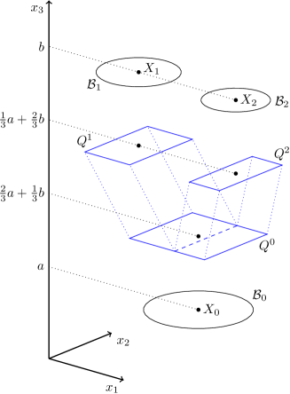
Figure 3: Construction around a branching point

Lemma 7.4.

Let $a\leq b\in\mathbb{R}$, $\gamma>0$, $X\in\mathbb{R}^{2}$, $\varphi>0$, and $R\geq 3$. Let then $Q\subseteq\mathbb{R}^{2}$ be a rectangle with side lengths $w$ and $h$ centered in $X$, such that $wh=\beta\varphi$, $w/h+h/w\leq\gamma$ and $\alpha^{-4/3}\beta^{-2/3}\leq\varphi$. Let as before $\eta:=\alpha^{-2/3}\beta^{1/6}$ be the coherence length.

Then there are $\rho\in L^{\infty}(\mathbb{R}^{2}\times[a,b];[0,1])$ and $B\in L^{2}(\mathbb{R}^{2}\times[a,b];\mathbb{R}^{3})$ such that $\mathrm{div}\,B=0$, $\rho B=0$, with $B=0$ and $\rho=1$ on $(\mathbb{R}^{2}\setminus\mathcal{B}^{\prime}(X,r))\times[a,b]$ for some $r\sim\eta R+\sqrt{\beta\varphi}$, and

$$\widetilde{F}^{(a,b)}_{\alpha,\beta}(\rho,B)\lesssim\sqrt{\varphi}|a-b|R^{2}+\frac{r^{2}}{|a-b|}\varphi R^{2},$$

where the implicit constants only depend on $\gamma$. Further, $\rho$ and $B$ satisfy the boundary conditions

$$\rho(x^{\prime},a)=v_{R}^{2}\left(\frac{|x^{\prime}-X|-\sqrt{\beta\varphi/\pi}}{\eta}\right),\hskip 28.45274pt\rho(x^{\prime},b)=\min\left\{1,\frac{\textup{dist}^{2}(x^{\prime},Q)}{\eta^{2}}\right\}\,,$$

and

$$B_{3}(x^{\prime},a)=\chi_{\mathcal{B}^{\prime}(X,\sqrt{\beta\varphi/\pi})}(x^{\prime})\,,\hskip 8.53581pt\text{ }\hskip 8.53581ptB_{3}(x^{\prime},b)=\chi_{Q}(x^{\prime})\,.$$

We note that our assumptions on the parameters $w,h,\varphi,$ just mean $w\sim h\sim\sqrt{\beta\varphi}\geq\eta$. That is, the thread diameter is large compared to the coherence length. Note that $r\sim\eta R+\sqrt{\beta\varphi}$ behaves like the maximum between the thread diameter $w\sim h$ and the cut-off scale $\eta R$. The proof of Lemma 7.4 is based on an explicit construction for a bilipschitz bijection with unit determinant that transforms a rectangle into a circle, which we first present.

Figure 4: The construction in Lemma 7.5 transforms a rectangle into a circle, keeping $\det\nabla^{\prime}u=1$. Each curve corresponds to a different value of $x_{3}$, and plots the solution of $\hat{r}(r,\theta)=t$, which corresponds to $r(\theta)=t/[\lambda(x_{3})\cos(\theta x_{3})]$ for $\theta\in(-\pi/4,\pi/4)$.

Lemma 7.5.

Assume that $z_{-},z_{+},h,w>0$, $X\in\mathbb{R}^{2}$ are given, $z_{-}<z_{+}$. Then there is $u:\mathbb{R}^{2}\times[z_{-},z_{+}]\to\mathbb{R}^{2}$ such that

$$u(x^{\prime},z_{-})=x^{\prime}\,,\hskip 14.22636ptu(X+(-\frac{1}{2}w,\frac{1}{2}w)\times(-\frac{1}{2}h,\frac{1}{2}h),z_{+})=\mathcal{B}^{\prime}(X,\sqrt{hw/\pi})\,,\hskip 14.22636pt\det\nabla^{\prime}u=1\text{ a.e.}\,.$$

The function $x\mapsto(u(x),x_{3})$ is bilipschitz, its inverse is of the form $y\mapsto(U(y),y_{3})$, and $u(X,x_{3})=X$ for all $x_{3}$. If additionally $h/w+w/h\leq\gamma$, then the bounds $|\nabla^{\prime}u|+|\nabla^{\prime}U|\lesssim 1$, $|\partial_{3}u|+|\partial_{3}U|\lesssim h/|z_{+}-z_{-}|$ hold, with constants which only depend on $\gamma$.

Proof.

By scaling and translation we may assume that $hw=\pi$, $z_{+}=1$, $z_{-}=0$, $X=0$. We can further assume $h=w=\sqrt{\pi}$, as the general case is obtained by taking the composition at each $x_{3}$ with the linear map $\mathop{\mathrm{diag}}(g(x_{3}),1/g(x_{3}))$, where $g(x_{3}):=\sqrt{h/w}(1-x_{3})+x_{3}$. We work in polar coordinates, and construct functions $\hat{r}$, $\hat{\theta}$ of $r$, $\theta$ and $x_{3}$ such that

$$u(r\cos\theta,r\sin\theta,x_{3})=(\hat{r}\cos\hat{\theta},\hat{r}\sin\hat{\theta}),$$

with $r\geq 0$ and $0\leq\theta\leq\pi/4$, and then extend by symmetry. We set

$$\hat{\theta}=f(\theta,x_{3})\,,\hskip 14.22636pt\hat{r}=r\lambda(x_{3})\cos(x_{3}\theta),$$

where $\lambda$ and $f$ are two functions still to be determined (see Figure 4). The extension of the $\frac{1}{8}-$sectors by reflection is feasible provided that $f(0,x_{3})=0$ and $f(\pi/4,x_{3})=\pi/4$ for all $x_{3}$, the boundary data are attained provided that $f(\theta,0)=\theta$, $\lambda(0)=1$, $\lambda(1)=2/\sqrt{\pi}$. The latter ensures that indeed the straight segment $r\cos\theta=\frac{w}{2}=\frac{\sqrt{\pi}}{2}$ is mapped into the unit circle $\hat{r}=1$. The determinant condition is equivalent to

$$1=\frac{\hat{r}}{r}\partial_{r}\hat{r}\partial_{\theta}f=\lambda^{2}(x_{3})\cos^{2}(x_{3}\theta)\partial_{\theta}f(\theta,x_{3}),$$

which can be solved (using $f(0,x_{3})=0$) to give

$$f(\theta,x_{3}):=\frac{1}{x_{3}\lambda^{2}(x_{3})}\tan(\theta x_{3})\,,$$

smoothly extended to $f(\theta,0)=\theta/\lambda^{2}(0)$. The condition $f(\pi/4,x_{3})=\pi/4$ determines $\lambda$,

$$\lambda(x_{3}):=\left(\frac{\tan(\pi x_{3}/4)}{\pi x_{3}/4}\right)^{1/2},$$

which obeys $\lambda(1)=2/\sqrt{\pi}$ and smoothly extends to $\lambda(0)=1$. Clearly $\lambda\sim 1$ so that $\partial_{\theta}f\sim 1$. This implies that the change of variables defines a smooth deformation of the $\frac{1}{8}-$sector which smoothly depends on $x_{3}\in[0,1]$. ∎

Proof of Lemma 7.4.

After a rotation and a translation, we may assume that $X=0$, $a=0$ and $b>0$; so that $Q=(-w/2,w/2)\times(-h/2,h/2)$. We treat two regions separately.

In the lower region $\mathbb{R}^{2}\times[0,b/2]$, we interpolate between $\mathcal{B}^{\prime}_{0}:=\mathcal{B}^{\prime}(0,\sqrt{\beta\varphi/\pi})$ and $Q$. To do this, let $u$ and $U$ be the functions from Lemma 7.5, using it for the rectangle $Q$ and $z_{-}=0$, $z_{+}=b/2$. The magnetic field is defined by

$$B_{3}(x):=\chi_{\mathcal{B}^{\prime}_{0}}(u(x))\,,\hskip 28.45274ptB^{\prime}(x):=\chi_{\mathcal{B}^{\prime}_{0}}(u(x))\partial_{3}U(u(x),x_{3})\hskip 8.53581pt\text{ for }x_{3}\in[0,b/2]\,.$$

The density is defined by

$$\rho(x):=v_{R}^{2}\left(\frac{|u(x)|-\sqrt{\beta\varphi/\pi}}{\eta}\right)\hskip 8.53581pt\text{ for }x_{3}\in[0,b/2]\,.$$

The condition $\rho B=0$ follows immediately, as well as the boundary data at $x_{3}=0$. Since $B=0$ and $\rho=1$ whenever $|u(x)|\geq\eta R+\sqrt{\beta\varphi/\pi}$ and since $|u(x)|\geq|x^{\prime}|/\|\nabla^{\prime}U\|_{\infty}$, we have $B=0$ and $\rho=1$ whenever $|x^{\prime}|\geq\|\nabla^{\prime}U\|_{\infty}(\eta R+\sqrt{\beta\varphi})$.

In order to check $\mathrm{div}\,B=0$, we fix $\psi\in C^{1}_{c}(\mathcal{B}^{\prime}_{r}\times(0,b/2))$. Performing then a change of variables at each $x_{3}$ gives, since $\det\nabla^{\prime}U=1$,

$$\int_{\mathbb{R}^{2}\times(0,b/2)}\left[\partial_{3}\psi B_{3}+\nabla^{\prime}\psi\cdot B^{\prime}\right]dx =\int_{\mathbb{R}^{2}\times(0,b/2)}(\partial_{3}\psi B_{3}+\nabla^{\prime}\psi\cdot B^{\prime})(U(y),y_{3})dy$$

$$=\int_{\mathbb{R}^{2}\times(0,b/2)}\chi_{\mathcal{B}^{\prime}_{0}}\left[\partial_{3}\psi(U(y),y_{3})+\partial_{3}U(y)\cdot\nabla^{\prime}\psi(U(y),y_{3}))\right]dy$$

$$=\int_{\mathcal{B}^{\prime}_{0}}\int_{(0,b/2)}\frac{d}{dx_{3}}(\psi(U(y),y_{3}))dy_{3}dy^{\prime}=0\,.$$

By the properties of $u$ we obtain $B_{3}(x^{\prime},b/2)=\chi_{Q}(x^{\prime})$.

In the upper region $\mathbb{R}^{2}\times[b/2,b]$, we keep $B(x^{\prime},x_{3}):=e_{3}\chi_{Q}(x^{\prime})$ concentrated on $Q$ and linearly interpolate the profile between $\rho^{1/2}(x^{\prime},b/2)$ and the profile $\rho^{1/2}(x^{\prime},b)$ given in the statement:

$$\rho^{1/2}(x):=\frac{2}{b}\left[\rho^{1/2}(x^{\prime},b/2)(b-x_{3})+\rho^{1/2}(x^{\prime},b)(x_{3}-b/2)\right]\hskip 8.53581pt\text{ for }x_{3}\in(b/2,b)\,.$$

It is immediate to check that $B_{3}$ and $\rho$ match continuously at all interfaces, $\rho B=0$ and $\mathrm{div}\,B=0$. This concludes the construction.

We estimate the energy similarly to the proof of Lemma 7.3. Lemma 7.5 gives $|\nabla^{\prime}u|\lesssim 1$, $|\partial_{3}u|\lesssim h/b$, $|\partial_{3}U|\lesssim h/b$, with constants depending only on $\gamma$. This yields $|B^{\prime}|\lesssim h/b$. Furthermore, by Lemma 7.2 $|v_{R}|\leq 1$ and $|\dot{v}_{R}|\leq 2$, so that $\rho\leq 1$, $|\nabla^{\prime}\rho^{1/2}|\lesssim 1/\eta$ and $|\partial_{3}\rho^{1/2}|\lesssim h/(\eta b)$.

We start with the region $x_{3}\in[0,b/2]$. All integrals in $x^{\prime}$ can be restricted to the set

$$\Omega_{x_{3}}:=\{x^{\prime}:\sqrt{\beta\varphi/\pi}\leq|u(x^{\prime},x_{3})|\leq\eta R+\sqrt{\beta\varphi/\pi}\}.$$

Since $\det\nabla u^{\prime}=1$, we have

$$|\Omega_{x_{3}}|=|\mathcal{B}^{\prime}(0,\eta R+\sqrt{\beta\varphi/\pi})\setminus\mathcal{B}^{\prime}_{0}|=\pi\eta^{2}R^{2}+2\sqrt{\beta\varphi\pi}\eta R\lesssim\eta\sqrt{\beta\varphi}R^{2},$$

(in the last step we used the assumption on $\varphi$ and $R\geq 3$). Therefore

$$\widetilde{F}_{\alpha,\beta}^{(0,b/2)}(\rho,B) \lesssim\int_{0}^{b/2}\int_{\Omega_{x_{3}}}\left(\frac{\alpha^{-2/3}\beta^{-1/3}}{\eta^{2}}+\frac{h^{2}\alpha^{-4/3}\beta^{-2/3}}{\eta^{2}b^{2}}+\alpha^{2/3}\beta^{-2/3}+\frac{h^{2}}{\beta b^{2}}\right)dx^{\prime}dx_{3}$$

$$\lesssim\int_{0}^{b/2}|\Omega_{x_{3}}|dx_{3}\left(\alpha^{2/3}\beta^{-2/3}+\frac{h^{2}}{\beta b^{2}}\right)$$

$$\lesssim\left(b+\frac{h^{2}}{b}\alpha^{-2/3}\beta^{-1/3}\right)R^{2}\sqrt{\varphi}\,$$

$$\lesssim\sqrt{\varphi}bR^{2}+\frac{r^{2}}{b}\varphi R^{2},$$

where in the last line we have used that $h^{2}\lesssim r^{2}$ and $\alpha^{-2/3}\beta^{-1/3}\lesssim\sqrt{\varphi}$. The region $(b/2,b)$ is simpler, as the $|B^{\prime}|^{2}$ term does not appear, the others are the same with the exception of $|\partial_{3}\rho^{1/2}|\lesssim 1/b$, which is smaller by the factor $\eta/h\lesssim 1$. ∎

Using this building block we can finally produce the construction that will be used at branching points.

Lemma 7.6.

Let $a<b\in\mathbb{R}$, $\gamma>0$, $\ell>0$, $R\geq 3$, $X_{i}\in\mathbb{R}^{2}$ and $\varphi_{i}>0$ for $i=0,1,2$ with $\varphi_{0}=\varphi_{1}+\varphi_{2}$, $\varphi_{0}/\varphi_{1}+\varphi_{0}/\varphi_{2}\leq\gamma$ and $\sqrt{\beta\varphi_{0}}\geq\eta$, where as above $\eta:=\alpha^{-2/3}\beta^{1/6}$.

Then, if $|X_{0}-X_{1}|,|X_{0}-X_{2}|\leq\ell/4$, $\sqrt{\beta\varphi_{0}}\ll|X_{1}-X_{2}|$ and $\eta R\ll\ell$, then there are $\rho\in L^{\infty}(\mathbb{R}^{2}\times[a,b];[0,1])$ and $B\in L^{2}(\mathbb{R}^{2}\times[a,b];\mathbb{R}^{3})$ such that $\mathrm{div}\,B=0$, $\rho B=0$, $B=0$ and $\rho=1$ on $(\mathbb{R}^{2}\setminus\mathcal{B}^{\prime}(X_{0},3\ell/4))\times[a,b]$,

$$\widetilde{F}^{(a,b)}_{\alpha,\beta}(\rho,B)\lesssim\sqrt{\varphi_{0}}|a-b|R^{2}+\frac{\ell^{2}}{|a-b|}\varphi_{0}R^{2},$$

where the implicit constants only depend on $\gamma$, and which satisfy the boundary conditions

$$\rho(x^{\prime},a)=v_{R}^{2}\left(\frac{|x^{\prime}-X_{0}|-\sqrt{\beta\varphi_{0}/\pi}}{\eta}\right)\hskip 2.84526pt\text{ }\hskip 2.84526pt\rho(x^{\prime},b)=\min_{i=1,2}v_{R}^{2}\left(\frac{|x^{\prime}-X_{i}|-\sqrt{\beta\varphi_{i}/\pi}}{\eta}\right)\,,$$

and

$$B_{3}(x^{\prime},a)=\chi_{\mathcal{B}^{\prime}(X_{0},\sqrt{\beta\varphi_{0}/\pi})}(x^{\prime})\,,\hskip 8.53581pt\text{ }\hskip 8.53581ptB_{3}(x^{\prime},b)=\sum_{i=1,2}\chi_{\mathcal{B}^{\prime}(X_{i},\sqrt{\beta\varphi_{i}/\pi})}(x^{\prime})\,.$$

Note that our assumptions on the parameters $\varphi_{0},\varphi_{1},\varphi_{2}$ and $h$ just mean that $\eta\lesssim\sqrt{\beta\varphi_{i}}\ll|X_{1}-X_{2}|\lesssim\ell$ and $\eta R\ll\ell$. That is, the thread diameter is at least as large as the coherence length $\eta$ but small compared to the distance between the threads. Likewise, $\ell$ is large compared to the cut-off scale $\eta R$.

Proof.

After a translation and a rotation we may assume that $a=0$, $b>0$, $X_{0}=0$, $X_{2}-X_{1}=\zeta e_{1}$, with $\zeta>0$. Let

$$w_{0}:=h:=(\beta\varphi_{0})^{1/2},\qquad w_{1}:=\frac{\varphi_{1}}{\varphi_{0}}w_{0}\qquad\textrm{ and }\qquad w_{2}:=\frac{\varphi_{2}}{\varphi_{0}}w_{0}.$$

Let then $Q^{i}:=X_{i}+[-w_{i}/2,w_{i}/2]\times[-h/2,h/2]$, for $i=0,1,2$. Notice that since $|X_{i}|\leq\ell/4$ and $w_{i}\leq w_{0}=h\ll\ell$, $Q^{i}\subseteq\mathcal{B}^{\prime}(3\ell/8)$.
We divide the interval $(0,b)$ in three parts (see again Figure 3). In $(0,b/3)$, we apply Lemma 7.4 to transform $\mathcal{B}^{\prime}(\sqrt{\beta\varphi_{0}/\pi})$ into $Q^{0}$ (in particular we have $\rho=1$ on $\left(\mathbb{R}^{2}\backslash\mathcal{B}^{\prime}(\frac{3\ell}{4})\right)\times(0,b/3)$). In $(b/3,2b/3)$, we connect $Q^{0}$ to $Q^{1}$ and $Q^{2}$ by an explicit construction (see below). Finally, in $(2b/3,b)$ we apply again Lemma 7.4 to transform $Q^{1}$ and $Q^{2}$ back into $\mathcal{B}^{\prime}(X_{1},\sqrt{\beta\varphi_{1}/\pi})$ and $\mathcal{B}^{\prime}(X_{2},\sqrt{\beta\varphi_{2}/\pi})$. Notice that in $(2b/3,b)$, if $\rho(x^{\prime},x_{3})\neq 1$ then by Lemma 7.4 and our hypothesis on the parameters, necessarily

$$|x^{\prime}|\leq\max_{i}|X_{i}|+O(\eta R+\sqrt{\beta\varphi_{0}})\leq\frac{\ell}{4}+o(\ell).$$

Thus, $\rho=1$ on $\left(\mathbb{R}^{2}\backslash\mathcal{B}^{\prime}(\frac{3\ell}{4})\right)\times(2b/3,b)$.

Figure 5: The construction in $(b/3,2b/3)$

It only remains to discuss the construction in the central region. Let $y_{1}:=X_{1}+w_{2}e_{1}/2$, $y_{2}:=X_{2}-w_{1}e_{1}/2$ and, for $i=1,2$, $\widetilde{Q}^{i}:=Q^{i}-y_{i}$, so that up to a null set, $Q^{0}$ is the disjoint union of $\widetilde{Q}^{1}$ and $\widetilde{Q}^{2}$ (see Figure 5). Since $y_{2}-y_{1}=X_{2}-X_{1}-w_{0}e_{1}/2$, and by assumption $w_{0}=(\beta\varphi_{0})^{1/2}\ll|X_{1}-X_{2}|$, we have $(y_{2}-y_{1})\cdot e_{1}>0$.
For $i=1,2$ and $x_{3}\in(b/3,2b/3)$ we set $\widetilde{Q}^{i}(x_{3}):=\widetilde{Q}_{i}+\frac{x_{3}-b/3}{b/3}y_{i}$. Since $(y_{2}-y_{1})\cdot e_{1}>0$, we have $\widetilde{Q}^{1}(x_{3})\cap\widetilde{Q}^{2}(x_{3})=\emptyset$ for all $x_{3}$. Furthermore, since $Q^{i}\subseteq\mathcal{B}^{\prime}(3\ell/8)$, also $\widetilde{Q}^{i}(x_{3})\subseteq\mathcal{B}^{\prime}(3\ell/8)$ for $x_{3}\in(b/3,2b/3)$. We finally let

$$\rho^{1/2}(x):=\min\left\{1,\eta^{-1}\textup{dist}(x^{\prime},\widetilde{Q}^{1}(x_{3})\cup\widetilde{Q}^{2}(x_{3}))\right\}\hskip 8.53581pt\text{ for }x_{3}\in[b/3,2b/3],$$

and correspondingly

$$(B^{\prime},B_{3})(x):=\sum_{i=1,2}\left(\frac{y_{i}}{b/3},1\right)\chi_{\widetilde{Q}^{i}(x_{3})}(x^{\prime})\,.$$

All admissibility conditions are easily checked. In particular, $\rho=1$ if $\textup{dist}(x^{\prime},\widetilde{Q}^{1}\cup\widetilde{Q}^{2}(x_{3}))\geq\eta$ which holds if $|x^{\prime}|\geq 3\ell/4$. The energy estimate is immediate. ∎

7.2 Boundary layer

Proposition 7.7.

Let $N\in\mathbb{N}$, $\alpha,\beta,T,t>0$ be given. Let $k:=\alpha^{1/3}\beta^{2/3}T$ and let $\varphi_{1},\dots,\varphi_{N^{2}}$ be positive numbers such that

$$k\varphi_{i}\in 2\pi\mathbb{N}\,\qquad\textrm{and }\qquad\sum_{i=1}^{N^{2}}\varphi_{i}=1.$$

Assume that in the regime $\beta\leq\alpha$, $\alpha\sqrt{2}/T\leq 1$, we have $t\gg\alpha^{-1}$, $1/N\gtrsim\alpha^{-2/3}\beta^{-1/3}$ and $\varphi_{i}\sim 1/N^{2}$ for every $i$. Then there are $\rho$ and $B$, admissible for $\widetilde{F}_{\alpha,\beta}^{(0,t)}$ and $k$-quantized, such that

$$\widetilde{F}_{\alpha,\beta}^{(0,t)}(\rho,B)\lesssim tN+\frac{1}{N^{2}t},$$ (7.6)

$$\alpha^{1/3}\beta^{7/6}\|\beta^{-1}{B_{3}}-1\|_{H^{-1/2}(x_{3}=0)}^{2}\lesssim\frac{\beta^{1/3}}{\alpha^{1/3}}+\frac{\beta^{1/2}}{N^{2}t}+\alpha^{1/3}\beta^{7/6},$$ (7.7)

and, denoting by $Q^{i}$ the squares centered in the $N^{2}$ points of the square grid of spacing $N^{-1}$ with $|Q^{i}|=\beta\varphi_{i}$,

$$B_{3}(x^{\prime},t)=\sum_{i}\chi_{Q^{i}}(x^{\prime})\text{ and }\rho^{1/2}(x^{\prime},t)=\min\{1,\eta^{-1}\textup{dist}(x^{\prime},\cup_{i}Q^{i})\}\,.$$ (7.8)

Note that the assumptions on the parameters $N$ and $\varphi_{i}$ mean that the sidelength $\sqrt{\beta\varphi_{i}}$ of the squares is larger than the coherence length $\alpha^{-2/3}\beta^{1/6}$ (see (3.9)) and that both of them are small compared to the distance (equal to $1/N$) between the squares. The assumption on the parameter $t$ means that the thickness $t$ of the boundary layer is large with respect to the coherence length, where we recall that vertical and horizontal lengths have different units.

Proof.

The key construction is described in [COS16, Lem. 4.7]. However, the notation and the scalings are different in that paper. Indeed, since there was no need to rescale $x_{3}$ by the thickness and $x^{\prime}$ by the distance between the threads $T\alpha^{-1/3}\beta^{-1/6}$, in that paper length was measured in terms of the penetration length. We first let $r_{i}$ be a square of side $1/N$ centered on the square grid of spacing $N^{-1}$, $Q^{i}\subseteq r_{i}$ be a square with the same center and area given by $|Q^{i}|=\beta\varphi_{i}$, and $b_{i}:=\beta\varphi_{i}N^{2}$. Denoting with a star the quantities from [COS16], we set $T_{*}:=Tt/2$, $\kappa_{*}:=\alpha\sqrt{2}/T$, $L_{*}:=T\alpha^{-1/3}\beta^{-1/6}$, $r_{i}^{*}:=L_{*}r_{i}$, $\hat{r}_{i}^{*}:=L_{*}Q^{i}$, $d_{0}^{*}:=L_{*}/N$, $\rho_{0}^{*}:=\beta^{1/2}L_{*}/N$, $N_{*}=N$, and $b_{i}^{*}:=(|\hat{r}_{i}^{*}|/|r_{i}^{*}|)\kappa_{*}/\sqrt{2}=b_{i}\kappa_{*}/\sqrt{2}$.

[COS16, Lem. 4.7] gives $Q_{L_{*}}$-periodic fields $\chi_{*}\in BV_{\mathrm{loc}}(\mathbb{R}^{2}\times(0,T_{*});\{0,1\})$ and $B_{*}=(B^{\prime}_{*},B_{3}^{*})\in L^{2}_{\mathrm{loc}}(\mathbb{R}^{3};\mathbb{R}^{3})$ such that $\mathrm{div}\,B_{*}=0$, $B_{*}(1-\chi_{*})=0$, and,

$$\chi_{*}(x^{\prime},T_{*})=\sum_{i}\chi_{\hat{r}_{i}^{*}}(x^{\prime})\qquad\textrm{and}\qquad B^{*}_{3}(x^{\prime},T_{*})=\frac{\kappa_{*}}{\sqrt{2}}\sum_{i}\chi_{\hat{r}_{i}^{*}}(x^{\prime})\hskip 14.22636pt\text{ for }x^{\prime}\in Q_{L_{*}}\,,$$

with energy

$$\frac{1}{L_{*}^{2}}\int_{Q_{L_{*}}\times(0,T_{*})}\kappa_{*}|D\chi_{*}|+|B_{*}^{\prime}|^{2}+\chi_{*}\left(B_{3}^{*}-\frac{\kappa_{*}}{\sqrt{2}}\right)^{2}dx\lesssim E_{*}^{int}:=\left(\frac{\kappa_{*}\rho_{0}^{*}T_{*}}{\sqrt{2}}+\frac{\kappa_{*}^{2}(\rho_{0}^{*}d_{0}^{*})^{2}}{2T_{*}}\right)\left(\frac{N}{L_{*}}\right)^{2}$$ (7.9)

and

$$\frac{1}{L_{*}^{2}}\|B_{3}^{*}-\sum_{i}b_{i}^{*}\chi_{q_{j}^{*}}\|^{2}_{H^{-1/2}(Q_{L_{*}})}\lesssim E_{*}^{ext}:=\left(\kappa_{*}(\rho_{0}^{*})^{2}+\frac{\kappa_{*}^{2}(\rho_{0}^{*})^{3}d_{0}}{T_{*}}\right)\left(\frac{N}{L_{*}}\right)^{2}\,.$$

We extend $\chi_{*}$ and $B_{*}$ to $Q_{L_{*}}\times(T_{*},2T_{*})$ by

$$\chi_{*}(x):=\chi_{*}(x^{\prime},T_{*})\qquad\textrm{and}\qquad B_{*}=(0,B_{3}^{*}(x^{\prime},T_{*}))\hskip 14.22636pt\text{ for }x^{\prime}\in Q_{L_{*}}\times(T_{*},2T_{*}),$$

so that (7.9) holds in $Q_{L_{*}}\times(0,2T_{*})$. We set

$$\rho_{*}(x):=\min\{1,\kappa_{*}^{2}d(x,\omega_{*})^{2}\},$$

where $\omega_{*}=\{x:\chi_{*}(x)=1\}$ (here $d(\cdot,\omega_{*})$ is the 3D distance, periodic in the tangential directions). Since $\omega_{*}$ is invariant in the $x_{3}-$direction inside $(T_{*},2T_{*})$ and since $t\gg\alpha^{-1}$, giving $T_{*}\gg\kappa_{*}^{-1}$, for $x_{3}=2T_{*}$,

$$\min\{1,\kappa_{*}^{2}d(x,\omega_{*})^{2}\}=\min\{1,\kappa_{*}^{2}\textup{dist}(x^{\prime},\omega_{*}\cap\{x_{3}=2T_{*}\})^{2}\}\qquad\textrm{for }x=(x^{\prime},2T_{*}).$$

Hence,

$$\rho_{*}(x^{\prime},2T_{*})=\min_{i}\left\{\min(1,\kappa_{*}^{2}\textup{dist}(x^{\prime},\hat{r}^{i}_{*})\right\}.$$

The same computation as in the proof of [COS16, Th. 4.9] leads to

$$\frac{1}{L_{*}^{2}}\int_{Q_{L_{*}}\times(0,2T_{*})}|\nabla\rho_{*}^{1/2}|^{2}+|B_{*}^{\prime}|^{2}+(B_{3}^{*}-\frac{\kappa_{*}}{\sqrt{2}}(1-\rho_{*}))^{2}dx\lesssim E_{*}^{int}\,.$$

We scale back in the tangential direction to obtain

$$\rho(x^{\prime},x_{3}):=\rho^{*}(L_{*}x^{\prime},x_{3})\quad\text{ and }\quad(B^{\prime},B_{3})(x^{\prime},x_{3}):=\frac{\sqrt{2}}{\kappa_{*}}\left(\frac{B^{\prime}_{*}}{L_{*}},B_{3}^{*}\right)(L_{*}x^{\prime},x_{3})\,.$$

We have $\mathrm{div}\,B=0$ and (7.8) holds. Changing variables gives $\nabla^{\prime}\rho^{1/2}(x)=L_{*}\nabla^{\prime}\rho_{*}^{1/2}(L_{*}x^{\prime},x_{3})$ and $\partial_{3}\rho^{1/2}(x)=\partial_{3}\rho^{1/2}_{*}(L_{*}x^{\prime},x_{3})$, so that

$$\widetilde{F}^{(0,t)}_{\alpha,\beta}(\rho,B)\leq\alpha^{-4/3}\beta^{-2/3}\frac{1}{L_{*}^{2}}\int_{Q_{L_{*}}\times(0,2T_{*})}|\nabla\rho_{*}^{1/2}|^{2}+|B^{\prime}_{*}|^{2}+\left(B_{3}^{*}-\frac{\kappa_{*}}{\sqrt{2}}(1-\rho_{*})\right)^{2}dx\\ \lesssim\alpha^{-4/3}\beta^{-2/3}E_{*}^{int}.$$

Since $E_{*}^{int}=\alpha^{4/3}\beta^{2/3}(Nt/2+2/(N^{2}t))$, this concludes the estimate for $\widetilde{F}^{(0,t)}_{\alpha,\beta}$.

We now estimate the boundary term. By the embedding of $L^{\infty}$ into $H^{-1/2}$ (recall that since $\sum_{i}\varphi_{i}=1$, $\int_{Q_{1}}\sum_{i}(b_{i}-\beta)\chi_{r_{i}}dx^{\prime}=0$) we have

$$\|\sum_{i}(b_{i}-\beta)\chi_{r_{i}}\|^{2}_{H^{-1/2}(Q_{1})}\lesssim\|b_{i}-\beta\|_{\infty}^{2}\,.$$

Rescaling the boundary estimate for $B_{3}^{*}$ leads to

$$\|B_{3}-\sum_{i}b_{i}\chi_{r_{i}}\|^{2}_{H^{-1/2}(Q_{1})}\lesssim\frac{1}{L_{*}^{3}}\frac{2}{\kappa_{*}^{2}}\|B_{3}^{*}-\sum_{i}b_{i}^{*}\chi_{r_{j}^{*}}\|^{2}_{H^{-1/2}(Q_{L_{*}})}\lesssim\frac{\beta^{7/6}}{\alpha^{2/3}}+\frac{\beta^{4/3}}{\alpha^{1/3}N^{2}t}$$

Adding terms and using that $\sum_{i}\chi_{r_{i}}\equiv 1$, we conclude that

$$\alpha^{1/3}\beta^{7/6}\|\beta^{-1}{B_{3}}-1\|_{H^{-1/2}(Q_{1})}^{2}\lesssim\frac{\beta^{1/3}}{\alpha^{1/3}}+\frac{\beta^{1/2}}{N^{2}t}+\frac{\alpha^{1/3}}{\beta^{5/6}}\|b_{i}-\beta\|_{\infty}^{2}\,.$$

∎

7.3 Back to the full GL functional

In this section, we relate the functional $\widetilde{F}_{\alpha,\beta}$, as defined in (7.3–7.4), with the functional $\widetilde{E}_{T}$, as defined in (1.5).

Proposition 7.8.

Let $k=\alpha^{1/3}\beta^{2/3}T$ and let $\rho,B$ be $k$-quantized admissible functions for $\widetilde{F}_{\alpha,\beta}$ with $\rho B=0$. Let $\omega:=\{\rho=0\}$ and then for $z\in(-1,1)$, $\omega_{z}:=\omega\cap\{x_{3}=z\}$. Assume that $\omega$ is closed, that $\omega^{c}$ is connected and that for every $x_{3}\in(-1,1)$, $\omega_{x_{3}}^{c}$ is also connected. Then, there is a pair $(u,A)$, admissible for $\widetilde{E}_{T}$, such that $\rho=|u|^{2}$, $B=\nabla\times A$, and

$$\widetilde{E}_{T}(u,A)=\widetilde{F}_{\alpha,\beta}(\rho,B).$$ (7.10)

Proof.

We shall construct a function $A$ on $\mathbb{R}^{2}\times(-1,1)$ so that $B=\nabla\times A$ everywhere, and then a multivalued function $\theta$ on the set $\Omega^{c}:=\mathbb{Z}^{2}\times\{0\}+\omega^{c}$ such that $\nabla\theta=\beta^{-1}kA$. Here $B$ and $\rho$ are $Q_{1}$-periodic, but $A$ and $\theta$ not necessarily. Setting $u:=\rho^{1/2}e^{i\theta}$ we then have $\nabla_{\beta^{-1}kA}u=e^{i\theta}\nabla\rho^{1/2}$, which directly implies (7.10). Notice that thanks to the hypothesis on $\omega$, the set $\Omega^{c}$ is a connected open set.

We start from the construction of $A$. By [COS16, Lem. 4.8] applied to $B-\beta e_{3}$ there is a $Q_{1}$-periodic potential $A_{\mathrm{per}}$ such that $\nabla\times A_{\mathrm{per}}=B-\beta e_{3}$ and $\textup{div}\,A=0$. We define $A(x):=A_{\mathrm{per}}(x)+\beta x_{1}e_{2}$ so that $\nabla\times A=B$. We remark that on any open set where $B=0$ the vector field $A$ is curl-free and divergence-free, therefore harmonic, and in particular smooth. In particular, since $\Omega^{c}$ is open and since by the Meissner condition, $B=0$ in $\Omega^{c}$, $A$ is smooth in $\Omega^{c}$.

We now turn to the existence of $\theta$. For a fixed level $x_{3}$, let $h+\omega^{i}_{x_{3}}$, $h\in\mathbb{Z}^{2}$, $i=1,...,I(x_{3})$ be the connected components of $(\mathbb{R}^{2}\times\{x_{3}\})\cap(\mathbb{Z}^{2}+\omega_{x_{3}})$. Denote the flux going through $\omega^{i}_{x_{3}}$ by

$$\Phi^{i}(x_{3}):=\int_{\omega^{i}_{x_{3}}}B_{3}\,dx^{\prime}.$$

By assumption we have

$$\beta^{-1}k\Phi^{i}(x_{3})\in 2\pi\mathbb{Z}\qquad\textrm{ for every $i$. }$$ (7.11)

Fix a smooth curve $\Gamma_{0}:=\{(\gamma_{0}(x_{3}),x_{3})\ :\ x_{3}\in(-1,1)\}\subseteq\Omega^{c}$. For $x_{3},y_{3}\in(-1,1)$, let $\Gamma_{0}^{x_{3},y_{3}}:=\{(\gamma_{0}(t),t)\ :\ t\in(x_{3},y_{3})\}\subseteq\Gamma_{0}$. For $x=(\gamma_{0}(x_{3}),x_{3})$, let $\theta(x):=\beta^{-1}k\int_{\Gamma_{0}^{0,x_{3}}}A\cdot\tau d\mathcal{H}^{1}$. Now, for a generic $x=(x^{\prime},x_{3})\in\Omega^{c}$, let

$$\theta(x):=\theta(\gamma_{0}(x_{3}),x_{3})+\beta^{-1}k\int_{\Gamma^{x}}A\cdot\tau d\mathcal{H}^{1},$$

where $\Gamma^{x}$ is any (horizontal) curve in $\Omega^{c}\cap(\mathbb{R}^{2}\times\{x_{3}\})$ connecting $x$ to $(\gamma_{0}(x_{3}),x_{3})$. This gives a well defined $\theta:\Omega^{c}\to\mathbb{R}/2\pi\mathbb{Z}$ since for every closed (horizontal) curve $\Gamma$ in $\Omega^{c}\cap(\mathbb{R}^{2}\times\{x_{3}\})$,

$$\beta^{-1}k\int_{\Gamma}A\cdot\tau d\mathcal{H}^{1}\in 2\pi\mathbb{Z}.$$ (7.12)

Indeed, this follows by Stokes’ Theorem and (7.11). Let us show that $\nabla\theta=\beta^{-1}kA$ in $\Omega^{c}$. Let $x=(x^{\prime},x_{3})$ be fixed and let $\Gamma^{x}$ be a fixed simple smooth curve joining $x$ to $(\gamma_{0}(x_{3}),x_{3})$ inside $\Omega^{c}\cap(\mathbb{R}^{2}\times\{x_{3}\})$. Since $\Omega^{c}$ is open, there is a simply connected neighborhood $V$ of $\Gamma^{x}$ such that $V\subseteq\Omega^{c}$. Let then $y=(y^{\prime},y_{3})\in V$. Upon shrinking $V$, we may assume that $(\gamma_{0}(y_{3}),y_{3})\in V$. Let $\Gamma^{y}\subseteq V$ be a smooth curve joining $y$ to $(\gamma_{0}(y_{3}),y_{3})$ and let $\Gamma^{x,y}\subseteq V$ be a smooth curve joining $x$ to $y$. By definition, we have

$$\theta(x)=\theta(\gamma_{0}(x_{3}),x_{3})+\beta^{-1}k\int_{\Gamma^{x}}A\cdot\tau d\mathcal{H}^{1},\quad\theta(y)=\theta(\gamma_{0}(y_{3}),y_{3})+\beta^{-1}k\int_{\Gamma^{y}}A\cdot\tau d\mathcal{H}^{1}$$

and

$$\theta(\gamma_{0}(y_{3}),y_{3})=\theta(\gamma_{0}(x_{3}),x_{3})+\beta^{-1}k\int_{\Gamma_{0}^{x_{3},y_{3}}}A\cdot\tau d\mathcal{H}^{1},$$

so that

$$\theta(y)-\theta(x)=\beta^{-1}k\int_{\Gamma^{y}}A\cdot\tau d\mathcal{H}^{1}+\beta^{-1}k\int_{\Gamma_{0}^{x_{3},y_{3}}}A\cdot\tau d\mathcal{H}^{1}-\beta^{-1}k\int_{\Gamma^{x}}A\cdot\tau d\mathcal{H}^{1}.$$

However, by Stokes Theorem (and $B=0$ in $V$),

$$\int_{\Gamma^{y}}A\cdot\tau d\mathcal{H}^{1}+\int_{\Gamma_{0}^{x_{3},y_{3}}}A\cdot\tau d\mathcal{H}^{1}-\int_{\Gamma^{x}}A\cdot\tau d\mathcal{H}^{1}=\int_{\Gamma^{x,y}}A\cdot\tau d\mathcal{H}^{1},$$

so that

$$\theta(y)-\theta(x)=\beta^{-1}k\int_{\Gamma^{x,y}}A\cdot\tau d\mathcal{H}^{1},$$

proving that indeed, $\nabla\theta=\beta^{-1}kA$ in $\Omega^{c}$. ∎

7.4 Proof of the upper bound

We start from a construction for an $N$-regular measure and finite $R$.

Proposition 7.9.

Let $\mu\in\mathcal{M}_{\mathrm{reg}}^{N}(Q_{1,1})$ for some $N\in\mathbb{N}$, $R\geq 3$, and assume (6.1) and (7.1) hold. Then, there exist sequences $u_{n}:Q_{1,1}\to\mathbb{C}$ and $A_{n}:Q_{1,1}\to\mathbb{R}^{3}$ such that

$$\limsup_{n\to+\infty}\,\widetilde{E}_{T}(u_{n},A_{n})\leq\frac{K_{R}}{K_{*}}I(\mu)+\frac{C}{N^{1/2}}(1+I(\mu)),$$ (7.13)

with $|u_{n}|$ and $\nabla\times A_{n}$ $Q_{1}-$periodic. Here $K_{R}$ and $K_{*}$ are as in Lemma 7.2, $C$ is universal. Moreover,

$$\limsup_{n\to+\infty}W_{2}^{2}(\beta^{-1}_{n}B^{n}_{3},\mu)\lesssim N^{-3/2}.$$ (7.14)

Proof.

We first modify slightly $\mu$ in order to be able to use Proposition 7.7 for the boundary layer. Set $\varepsilon_{N}:=N^{-3/2}$. For $x_{3}\in[-1+\varepsilon_{N},1-\varepsilon_{N}]$ let $\hat{\mu}_{x_{3}}:=\mu_{x_{3}/(1-\varepsilon_{N})}$ and for $x_{3}\in[-1,-1+\varepsilon_{N}]\cup[1-\varepsilon_{N},1]$, let $\hat{\mu}_{x_{3}}:=\mu_{1}=\mu_{-1}=N^{-2}\sum_{l}\delta_{X_{l}}$, where the $\{X_{l}\}_{l=1}^{N^{2}}$ form a regular grid with spacing $1/N$ (recall Def. 5.14). We then have

$$I(\hat{\mu})\leq\frac{1}{1-\varepsilon_{N}}I(\mu)+2K_{*}\varepsilon_{N}N.$$

Moreover, since $|\hat{\mu}|(Q_{1}\times(1-\varepsilon_{N},1))=\varepsilon_{N}$, the same on the other side, and

$$W_{2}^{2}((1-\varepsilon_{N})\mu,\hat{\mu}{\mathchoice{\>\hbox{\vrule width=0.2pt\vbox to7.0pt{\vfill\hrule width=7.0pt,height=0.2pt}}\>}{\>\hbox{\vrule width=0.2pt\vbox to7.0pt{\vfill\hrule width=7.0pt,height=0.2pt}}\>}{\,\hbox{\vrule width=0.2pt\vbox to5.0pt{\vfill\hrule width=5.0pt,height=0.2pt}}\,}{\,\hbox{\vrule width=0.2pt\vbox to3.35pt{\vfill\hrule width=3.35pt,height=0.2pt}}\,}}(Q_{1}\times(-1+\varepsilon_{N},1-\varepsilon_{N}))\lesssim\varepsilon_{N}^{2},$$

so that

$$W_{2}^{2}(\mu,\hat{\mu})\lesssim\varepsilon_{N}+\varepsilon^{2}_{N}\lesssim N^{-3/2},$$

it is enough to prove the estimates for $\hat{\mu}$ instead of $\mu$.

We start by characterizing the geometry of the construction, which will not depend on $n$. The measure $\hat{\mu}$ is supported on finitely many polygonal curves, parametrized by $X_{i}:[a_{i},b_{i}]\to Q_{1}$, which are disjoint up to the endpoints and carry a flux $\varphi_{i}>0$. The endpoints are either on the boundary of $Q_{1,1}$, or they are triple points. Those on the boundary constitute a regular grid. We let $\varphi_{\mathrm{min}}:=\min_{i}\varphi_{i}$, $\varphi_{\mathrm{max}}:=\max_{i}\varphi_{i}$, and $\gamma:=8\varphi_{\mathrm{max}}/\varphi_{\mathrm{min}}$. Since there are finitely many curves, these quantities are finite and positive. We define as before $\eta_{n}:=\alpha_{n}^{-2/3}\beta_{n}^{1/6}$ to be the coherence length; by (6.1) we have $\eta_{n}\to 0$.

Let $y_{j}:=(Y_{j},z_{j})\in Q_{1,1}$ denote the internal endpoints of the curves. For $\ell>0$ sufficiently small one has that, for any $j$, the only curves which intersect $\mathcal{B}^{\prime}_{\ell}(Y_{j})\times(z_{j}-\ell,z_{j}+\ell)$ are those with an endpoint in $y_{j}$. Since $y_{j}$ is a triple point, there are three such curves $\Gamma_{0}$, $\Gamma_{1}$ and $\Gamma_{2}$, intersecting only at $y_{j}$. If we let $M$ be the maximal slope of all curves and $t_{\ell}:=\ell/(8M)$, then no curve intersects $\partial\mathcal{B}^{\prime}_{\ell/8}(Y_{j})\times(z_{j}-t_{\ell},z_{j}+t_{\ell})$ (this means, they all “exit” from the top and bottom faces). Without loss of generality, we can assume that $(X_{0},z_{j}-t_{\ell})=\Gamma_{0}\cap\left(\mathcal{B}^{\prime}(Y_{j},\ell)\times\{z_{j}-t_{\ell}\}\right)$, $(X_{1},z_{j}+t_{\ell})=\Gamma_{1}\cap\left(\mathcal{B}^{\prime}(Y_{j},\ell)\times\{z_{j}+t_{\ell}\}\right)$ and $(X_{2},z_{j}+t_{\ell})=\Gamma_{2}\cap\left(\mathcal{B}^{\prime}(Y_{j},\ell)\times\{z_{j}+t_{\ell}\}\right)$ (see Figure 6). By definition of $t_{\ell}$, it holds $|X_{0}-Y_{j}|\leq\frac{\ell}{8}$ and $|X_{i}-X_{0}|\leq\frac{\ell}{4}$ for $i=1,2$. We set $\omega_{j}:=\mathcal{B}^{\prime}_{\ell}(Y_{j})\times(z_{j}-t_{\ell},z_{j}+t_{\ell})$ and let $\delta_{\ell}$ be the minimum distance between any two curves outside $\cup_{j}\omega_{j}$.

Figure 6: The construction in $(b/3,2b/3)$

To explain the strategy, we first carry out a construction which ignores quantization. For sufficiently large $n$ we have $\eta_{n}R+\sqrt{\varphi_{\mathrm{max}}\beta_{n}/\pi}<\delta_{\ell}/2$ and can thus use the construction of Lemma 7.3 in a $\delta_{\ell}/2$-neighborhood of each curve (outside of $\cup_{j}\omega_{j}$), extending by $\rho_{n}=1$ and $B_{n}=0$ to the complement. In the cylinders $\omega_{j}$, since the geometry is fixed, for $n$ sufficiently large the conditions $\sqrt{\beta_{n}\varphi_{\mathrm{min}}}\geq\eta_{n}$, $\sqrt{\beta_{n}\varphi_{\mathrm{max}}}\ll|X_{1}-X_{2}|$ and $\eta_{n}R\ll\ell$ are satisfied and we can use Lemma 7.6. We then have that $\rho_{n}=1$ outside $\mathcal{B}^{\prime}(X_{0},3\ell/4)\times(z_{j}-t_{\ell},z_{j}+t_{\ell})\subseteq\omega_{j}$.

In order to obtain a quantized field, we define $k_{n}$ as in (7.2), which obeys $k_{n}\in 2\pi\mathbb{N}$ and $k_{n}\to+\infty$. Let $\hat{\mu}^{n}$ be the $k_{n}$-quantized approximation of $\hat{\mu}$, as given by Lemma 5.18. For sufficiently large $n$ we have $\frac{1}{2}\hat{\mu}\leq\hat{\mu}^{n}\leq 2\hat{\mu}$ and for $|x_{3}|\geq 1-\varepsilon_{N}$,

$$\hat{\mu}_{x_{3}}^{n}=\sum_{l}\varphi_{l}^{n}\delta_{X_{l}},$$

where $|\varphi_{l}^{n}-1/N^{2}|\leq C(\hat{\mu})/k_{n}$, $\varphi_{l}^{n}\leq 2/N^{2}$. The fluxes $\varphi_{i}^{n}$ obey $\frac{1}{2}\varphi_{i}\leq\varphi_{i}^{n}\leq 2\varphi_{i}$.

We then construct $B_{n}$ and $\rho_{n}$ using Lemma 7.3 and Lemma 7.6 as discussed above. The geometry is the one determined by $\hat{\mu}$. In particular, the points $y_{j}$, and the constants $M$, $\varphi_{\mathrm{min}}$, $\varphi_{\mathrm{max}}$, $\delta_{\ell}$ and $t_{\ell}$ do not depend on $n$, and only $\delta_{\ell}$ and $t_{\ell}$ depend on $\ell$. Adding terms gives for sufficiently large $n$ (as a geometry dependent function of $\ell$ and $R$)

$$\widetilde{F}_{\alpha_{n},\beta_{n}}^{(-1,1)}(\rho_{n},B_{n})\leq \sum_{i}\left(1+\frac{C}{(\varphi_{i}^{n}\alpha_{n}^{4/3}\beta_{n}^{2/3})^{1/2}}+\frac{C}{\varphi_{i}^{n}\alpha_{n}^{4/3}\beta_{n}^{2/3}}\right)\int_{a_{i}}^{b_{i}}\bigl{(}K_{R}\sqrt{\varphi_{i}^{n}}+\varphi_{i}^{n}|\dot{X}_{i}|^{2}\bigr{)}dx_{3}$$

$$+C(\gamma)\sum_{j}\sqrt{\varphi_{\mathrm{max}}}t_{\ell}R^{2}+\frac{\ell^{2}}{t_{\ell}}\varphi_{\mathrm{max}}R^{2},$$

where the first sum runs over all curves and the second over the cylinders and where $C(\gamma)>0$ is a constant depending on $\gamma$. In the limit $n\to+\infty$ we have $\varphi_{i}^{n}\to\varphi_{i}$, $\alpha_{n}^{2}\beta_{n}\to+\infty$ and therefore, inserting the definition of $t_{\ell}$,

$$\limsup_{n\to+\infty}\widetilde{F}_{\alpha_{n},\beta_{n}}^{(-1,1)}(\rho_{n},B_{n})\leq \sum_{i}\int_{a_{i}}^{b_{i}}\bigl{(}K_{R}\sqrt{\varphi_{i}}+\varphi_{i}|\dot{X}_{i}|^{2}\bigr{)}dx_{3}+C(\gamma)R^{2}\ell\sum_{j}\left(\frac{\sqrt{\varphi_{\mathrm{max}}}}{M}+M\varphi_{\mathrm{max}}\right)\,.$$

The sum over $j$ depends only on $\hat{\mu}$. Therefore if $\ell$ is chosen sufficiently small we have

$$\limsup_{n\to+\infty}\,\widetilde{F}_{\alpha,\beta}^{(-1,1)}(\rho_{n},B_{n})\leq\frac{K_{R}}{K_{*}}I(\mu)+\frac{1}{N^{1/2}}\,.$$

Moreover, thanks to (7.5) and Lemma 5.18, we have

$$W_{2}^{2}(\beta^{-1}_{n}B^{n}_{3},\hat{\mu}) \lesssim W_{2}^{2}(\beta^{-1}_{n}B^{n}_{3},\hat{\mu}^{n})+W_{2}^{2}(\hat{\mu},\hat{\mu}^{n})$$

$$\lesssim C(\hat{\mu})\beta_{n}+t_{\ell}\,\sharp\{Y_{j}\}+C(\hat{\mu})k_{n}^{-1}$$

$$\lesssim C(\hat{\mu})\beta_{n}+\frac{\ell}{M}\,\sharp\{Y_{j}\}+C(\hat{\mu})k_{n}^{-1}.$$

Again, since $\sharp\{Y_{j}\}/M$ only depends on $\hat{\mu}$, if we choose $\ell$ sufficiently small then

$$\limsup_{n\to+\infty}W_{2}^{2}(\beta^{-1}_{n}B^{n}_{3},\hat{\mu})\leq N^{-3/2}.$$ (7.15)

We finally address the boundary layer, focusing for definiteness on the side $x_{3}>0$. We first apply once more Lemma 7.4 to each curve for $x_{3}\in(1-\varepsilon_{N},1-\varepsilon_{N}/2)$, so that the resulting fields $B_{n}$ and $\rho_{n}$ obey for all $x_{3}\in(1-\varepsilon_{N}/2,1)$,

$$B_{n}(x)=\sum_{l}e_{3}\chi_{Q^{l}}(x^{\prime})\text{ and }\rho_{n}(x)=\min\{1,\eta_{n}^{-1}\textup{dist}(x^{\prime},\cup_{l}Q^{l})\},$$

where $Q^{l}$ are squares centered in the $N^{2}$ points $X_{l}$ with $|Q^{l}|=\beta\varphi_{l}^{n}$ , and $|\varphi_{l}^{n}-1/N^{2}|\leq C(\hat{\mu})/k_{n}$. Then we modify $\rho_{n}$ and $B_{n}$ in the set $x_{3}\in(1-\varepsilon_{N}/2,1)$ using Proposition 7.7. This results in new fields $\hat{\rho}_{n}$, $\hat{B}_{n}$ which obey

$$\widetilde{F}_{\alpha_{n},\beta_{n}}^{(1-\varepsilon_{N}/2,1)}(\hat{\rho}_{n},\hat{B}_{n})+\alpha_{n}^{1/3}\beta_{n}^{7/6}\|\beta_{n}^{-1}{(\hat{B}_{n})_{3}}-1\|_{H^{-1/2}(x_{3}=1)}^{2}\lesssim\frac{1}{N^{1/2}}+\frac{\beta_{n}^{1/3}}{\alpha_{n}^{1/3}}+\frac{\beta_{n}^{1/2}}{N^{1/2}}+\frac{\alpha_{n}^{1/3}}{\beta_{n}^{5/6}}\frac{C(\hat{\mu})N^{4}}{k_{n}^{2}}\,.$$

By (6.1) and (7.2) all terms up to the first one tend to zero as $n\to+\infty$. Therefore

$$\limsup_{n\to+\infty}\,\widetilde{F}_{\alpha_{n},\beta_{n}}(\hat{\rho}_{n},\hat{B}_{n})\leq\frac{K_{R}}{K_{*}}I(\hat{\mu})+\frac{C}{N^{1/2}}\,.$$

Finally, we pass from $(\hat{\rho}_{n},\hat{B}_{n})$ to $(u_{n},A_{n})$ via Proposition 7.8 and conclude the proof of (7.13). We also obtain (7.14) since

$$W^{2}_{2}(\beta^{-1}_{n}(\hat{B}_{n})_{3},\hat{\mu})\lesssim W^{2}_{2}(\beta^{-1}_{n}B^{n}_{3},\hat{\mu})+N^{-3/2}.$$

∎

It only remains to combine the different steps.

Proof of Proposition 7.1.

By density (Theorem 5.15) there is a sequence $\mu^{N}\in\mathcal{M}_{\mathrm{reg}}^{N}(Q_{1,1})$ of $N$-regular measures converging weakly to $\mu$, with $\limsup_{N\to+\infty}I(\mu^{N})\leq I(\mu)$. Fix $R\geq 3$ and let $(u_{n}^{N},A_{n}^{N})$ be as in Proposition 7.9. Taking a diagonal subsequence (first with $N$, then with $R$) we obtain

$$\limsup_{n\to+\infty}\,\widetilde{E}_{T}(u_{n}^{N(n)},A_{n}^{N(n)})\leq I(\mu),$$

and $\beta_{n}^{-1}(B_{n}^{N(n)})_{3}\rightharpoonup\mu$. From the compactness statement of Proposition 6.1 and uniqueness of $m$ one obtains $\beta_{n}^{-1}(B_{n}^{N(n)})^{\prime}\rightharpoonup m$ and $\beta_{n}^{-1}(1-|u_{n}^{N(n)}|^{2})\rightharpoonup\mu$. ∎

References

- [ACO09] G. Alberti, R. Choksi, and F. Otto. Uniform energy distribution for an isoperimetric problem with long-range interactions. J. Amer. Math. Soc., 22:569–605, 2009.
- [AFP00] L. Ambrosio, N. Fusco, and D. Pallara. Functions of bounded variation and free discontinuity problems. Oxford Mathematical Monographs. Oxford University Press, New York, 2000.
- [AGS05] L. Ambrosio, N. Gigli, and G. Savaré. Gradient flows in metric spaces and in the space of probability measures. Lectures in Mathematics ETH Zürich. Birkhäuser Verlag, Basel, 2005.
- [BCDM00] H. Ben Belgacem, S. Conti, A. DeSimone, and S. Müller. Rigorous bounds for the Föppl-von Kármán theory of isotropically compressed plates. J. Nonlinear Sci., 10:661–683, 2000.
- [BCDM02] H. Ben Belgacem, S. Conti, A. DeSimone, and S. Müller. Energy scaling of compressed elastic films. Arch. Rat. Mech. Anal., 164:1–37, 2002.
- [BCM09] M. Bernot, V. Caselles, and J.-M. Morel. Optimal transportation networks, volume 1955 of Lecture Notes in Mathematics. Springer-Verlag, Berlin, 2009. Models and theory.
- [Bet14] F. Bethuel. A counterexample to the weak density of smooth maps between manifolds in Sobolev spaces. arXiv:1401.1649, 2014.
- [BG15] P. Bella and M. Goldman. Nucleation barriers at corners for a cubic-to-tetragonal phase transformation. Proc. Roy. Soc. Edinburgh Sect. A, 145:715–724, 2015.
- [Bra02] A. Braides. -convergence for beginners, volume 22 of Oxford Lecture Series in Mathematics and its Applications. Oxford University Press, Oxford, 2002.
- [BRW16] A. Brancolini, C. Rossmanith, and B. Wirth. Optimal micropatterns in 2d transport networks and their relation to image inpainting, 2016.
- [BW15] A. Brancolini and B. Wirth. Optimal micropatterns in transport networks, 2015.
- [CC15] A. Chan and S. Conti. Energy scaling and branched microstructures in a model for shape-memory alloys with invariance. Math. Models. Metods App. Sci., 25:1091–1124, 2015.
- [CCKO08] R. Choksi, S. Conti, R. V. Kohn, and F. Otto. Ground state energy scaling laws during the onset and destruction of the intermediate state in a type-I superconductor. Comm. Pure Appl. Math., 61:595–626, 2008.
- [CDZ17] S. Conti, J. Diermeier, and B. Zwicknagl. Deformation concentration for martensitic microstructures in the limit of low volume fraction. Calc. Var. Partial Differential Equations, 56:56:16, 2017.
- [CKO99] R. Choksi, R. V. Kohn, and F. Otto. Domain branching in uniaxial ferromagnets: a scaling law for the minimum energy. Comm. Math. Phys., 201:61–79, 1999.
- [CKO04] R. Choksi, R. V. Kohn, and F. Otto. Energy minimization and flux domain structure in the intermediate state of a type-I superconductor. Journal of Nonlinear Science, 14:119–171, 2004.
- [CO16] E. Cinti and F. Otto. Interpolation inequalities in pattern formation. J. Funct. Anal., 271:3348–3392, 2016.
- [Con00] S. Conti. Branched microstructures: scaling and asymptotic self-similarity. Comm. Pure Appl. Math., 53:1448–1474, 2000.
- [COS16] S. Conti, F. Otto, and S. Serfaty. Branched microstructures in the Ginzburg-Landau model of type-I superconductors. SIAM J. Math. Anal., 48:2994–3034, 2016.
- [CZ16] S. Conti and B. Zwicknagl. Low volume-fraction microstructures in martensites and crystal plasticity. Math. Models Methods Appl. Sci., 26:1319–1355, 2016.
- [DM93] G. Dal Maso. An introduction to -convergence. Progress in Nonlinear Differential Equations and their Applications, 8. Birkhäuser Boston Inc., Boston, MA, 1993.
- [FHSS12] R. L. Frank, C. Hainzl, R. Seiringer, and J. P. Solovej. Microscopic derivation of Ginzburg-Landau theory. J. Amer. Math. Soc., 25:667–713, 2012.
- [GM15] M. Goldman and B. Merlet. Phase segregation for binary mixtures of Bose-Einstein Condensates. preprint, 2015.
- [Gol17] M. Goldman. Self-similar minimizers of a branched transport functional. preprint, 2017.
- [JS01] W. Jin and P. Sternberg. Energy estimates of the von Kármán model of thin-film blistering. J. Math. Phys., 42:192–199, 2001.
- [JT80] A. Jaffe and C. Taubes. Vortices and monopoles, volume 2 of Progress in Physics. Birkhäuser, Boston, Mass., 1980. Structure of static gauge theories.
- [KKO13] H. Knüpfer, R. V. Kohn, and F. Otto. Nucleation barriers for the cubic-to-tetragonal phase transformation. Comm. Pure Appl. Math., 66:867–904, 2013.
- [KM92] R. V. Kohn and S. Müller. Branching of twins near an austenite-twinned-martensite interface. Phil. Mag. A, 66:697–715, 1992.
- [KM94] R. V. Kohn and S. Müller. Surface energy and microstructure in coherent phase transitions. Comm. Pure Appl. Math., 47:405–435, 1994.
- [KM11] H. Knüpfer and C. B. Muratov. Domain structure of bulk ferromagnetic crystals in applied fields near saturation. J. Nonlinear Sci., 21:921–962, 2011.
- [Mod87] L. Modica. The gradient theory of phase transitions and the minimal interface criterion. Arch. Rat. Mech. Anal., 98:123–142, 1987.
- [OS11] E. Oudet and F. Santambrogio. A Modica-Mortola approximation for branched transport and applications. Arch. Ration. Mech. Anal., 201:115–142, 2011.
- [OV10] F. Otto and T. Viehmann. Domain branching in uniaxial ferromagnets: asymptotic behavior of the energy. Calc. Var. Partial Differential Equations, 38:135–181, 2010.
- [PGPP05] R. Prozorov, R. W. Giannetta, A. A. Polyanskii, and G. K. Perkins. Topological hysteresis in the intermediate state of type I superconductors. Phys. Rev. B, 72:212508, 2005.
- [PH09] R. Prozorov and J. Hoberg. Dynamic formation of metastable intermediate state patterns in type-I superconductors. 25th International Conference on Low Temperature Physics, Journal of Physics: Conference Series, 150, 2009.
- [Pro07] R. Prozorov. Equilibrium topology of the intermediate state in type-I superconductors of different shapes. Phys. Rev. Lett., 98:257001, 2007.
- [Ser15] S. Serfaty. Coulomb gases and Ginzburg-Landau vortices. Zurich Lectures in Advanced Mathematics. European Mathematical Society (EMS), Zürich, 2015.
- [SS07] E. Sandier and S. Serfaty. Vortices in the magnetic Ginzburg-Landau model. Progress in Nonlinear Differential Equations and their Applications, 70. Birkhäuser Boston, Inc., Boston, MA, 2007.
- [Tin96] M. Tinkham. Introduction to superconductivity. Int. series in Pure and Appl. physics. McGraw Hill, New York, 1996.
- [Vie09] T. Viehmann. Uniaxial Ferromagnets. PhD thesis, Universität Bonn, 2009.
- [Vil03] C. Villani. Topics in optimal transportation, volume 58 of Graduate Studies in Mathematics. American Mathematical Society, Providence, RI, 2003.
- [Xia04] Q. Xia. Interior regularity of optimal transport paths. Calc. Var. Partial Differential Equations, 20:283–299, 2004.
- [Zwi14] B. Zwicknagl. Microstructures in low-hysteresis shape memory alloys: Scaling regimes and optimal needle shapes. Arch. Ration. Mech. Anal., 213:355–421, 2014.