Wave propagation and shock formation in the most general scalar-tensor theories

Abstract

This work studies wave propagation in the most general scalar-tensor theories, particularly focusing on the causal structure realized in these theories and also the shock formation process induced by nonlinear effects. For these studies we use the Horndeski theory and its generalization to the two scalar field case. We show that propagation speeds of gravitational wave and scalar field wave in these theories may differ from the light speed depending on background field configuration, and find that a Killing horizon becomes a boundary of causal domain if the scalar fields share the symmetry of the background spacetime. About the shock formation, we focus on transport of discontinuity in second derivatives of the metric and scalar field in the shift-symmetric Horndeski theory. We find that amplitude of the discontinuity generically diverges within finite time, which corresponds to shock formation. It turns out that the canonical scalar field and the scalar DBI model, among other theories described by the Horndeski theory, are free from such shock formation even when the background geometry and scalar field configuration are nontrivial. We also observe that gravitational wave is protected against shock formation when the background has some symmetries at least. This fact may indicate that the gravitational wave in this theory is more well-behaved compared to the scalar field, which typically suffers from shock formation.

I Introduction

Theories of gravitation modified by scalar degrees of freedom have a long history of study, and nowadays such theories are utilized in various research fields including gravitational physics and cosmology. Just to list some of the applications, inflation describing our universe in the earliest era Starobinsky (1980); *Sato:1980yn; *Guth:1980zm is typically realized using a scalar field called inflaton that is coupled to gravity. Also, many attempts have been made to explain the accelerated expansion of our universe at late time Schmidt et al. (1998); *Riess:1998cb; *Perlmutter:1998np by modifying gravitation at cosmologically large scale rather than by attributing it to the cosmological constant, whose origin it yet to be known. For these modifications to be viable, they must be consistent with various tests of gravity at scales ranging from sub-millimeter to astrophysical ones. To conduct such experimental tests and also to examine their theoretical consistencies, behaviors of gravity and scalar fields in those modified theories have been studied from various viewpoints as reviewed in, e.g., Ref. Clifton et al. (2012).

Quite a number of such gravitation theories with modifications has been proposed by now, and then it is desirable to have a theory that could be used as a framework to treat them in a unified manner. Such a theory must be free from pathological behaviors including ghost instability, and also it should encompass a wide variety of other theories as its subclass. Within this context, the Galileon theory was proposed as a theory that is free from the Ostrogradsky ghost instability although its Lagrangian contains higher derivative terms Nicolis et al. (2009). Later on, this theory was covariantized to include gravity and also was generalized to incorporate more parameters into the theory by Deffayet et al. (2009, 2011). The resultant theory was dubbed the generalized Galileon theory, which was shown by Kobayashi et al. (2011) to be equivalent to the Horndeski theory Horndeski (1974) constructed in 1970’s as a generalization of Lovelock theories of gravity Lovelock (1971). This theory has been studied in wide variety of contexts in cosmology and gravitational physics, e.g. by Kobayashi et al. (2011) which pursued inflation scenario based on it.

The Horndeski theory is the most general scalar-tensor theory with a single scalar field whose Euler-Lagrange equation has derivatives of the metric and the scalar field only up to second order. There are a several ways to extend this theory further. One of the simplest extensions would be to incorporate multiple scalar fields into the theory, which was realized in the generalized multi-Galileon theory Padilla et al. (2010, 2011a); Hinterbichler et al. (2010); Padilla et al. (2011b); Padilla and Sivanesan (2013). Later on, it was realized that the multi-DBI inflation models Renaux-Petel (2011); Renaux-Petel et al. (2011); Koyama et al. (2014); Langlois et al. (2008a, b) are not included in this theory Kobayashi et al. (2013), which motivated to construct the two scalar field version of the Horndeski theory based on the derivation in the single scalar field case. Such a construction was attempted in Ohashi et al. (2015). As a result, the most general equations of motion of such a theory was successfully constructed, while the Lagrangian corresponding to those equations has not been found so far. We call this theory the bi-Horndeski theory in this work. There are also some other theories with multiple scalar fields proposed based on different methods (see e.g. Padilla et al. (2014); Saridakis and Tsoukalas (2016a, b); Allys (2016); Akama and Kobayashi (2017)) as well as generalized theories for vector fields Horndeski (1976); Deffayet et al. (2014); Tasinato (2014); Heisenberg (2014); Allys et al. (2016); Beltran Jimenez and Heisenberg (2016a, b).

Another type of extension is to construct scalar-tensor theories that encompass the Horndeski theory as their subclass. Such a theory was first introduced in Zumalacarregui and Garcia-Bellido (2014); Gleyzes et al. (2015a, b), where a subclass of the extended theory was related to the Horndeski theory by disformal transformation. This theory was dubbed the beyond-Horndeski theory, and later on it was extended further to incorporate higher order terms in Lagrangian without re-introducing the ghost instability in Gao (2014); Deffayet et al. (2015); Domenech et al. (2015); Langlois and Noui (2016a, b); Crisostomi et al. (2016a, b); Ben Achour et al. (2016a); Ezquiaga et al. (2016); Motohashi et al. (2016); de Rham and Matas (2016); Ben Achour et al. (2016b); Crisostomi et al. (2017); Langlois et al. (2017). There are similar extended theories involving vector degrees of freedom and also derivatives of spacetime curvature Heisenberg et al. (2016); Naruko et al. (2016), which have been attracting wide interest recently.

In this work, among the extended theories mentioned above, we focus on the Horndeski theory and also the bi-Horndeski theory. The latter is related to various other theories such as the Horndeski theory and the multi-Galileon theory as shown in appendix B, hence the results obtained for this theory will be applicable to those theories as well. Also, the mathematical structure of these theories are relatively simpler and then easier to deal with compared to the other extended theories mentioned above. Adding to that, the Horndeski theory is known to be related to Gauss-Bonnet and Lovelock theories of gravity in higher dimensions via dimensional reduction (see e.g. Charmousis et al. (2012); Charmousis (2015)). This fact suggests that some properties of these higher-dimensional theories, such as those studied in Izumi (2014); Reall et al. (2014, 2015), may persist even in the bi-Horndeski theory and its descendants.

One of the most basic properties of a theory is the wave propagation speed, since it governs the wave dynamics and also the causal structure of that theory. In the general relativity (GR) with a minimally-coupled canonical scalar field, the situation is relatively simple because any wave simply propagates at the speed of light. However, in the Horndeski theory and its generalizations, propagation speeds of the gravitational wave and scalar field wave may differ from the speed of light, and also they may depend on the environment, that is, the background field configuration on which the wave propagates. Phenomena associated with wave propagation in extended gravity theories have been studied in various contexts (see e.g. Adams et al. (2006); Babichev et al. (2006, 2008); Appleby and Linder (2012); Neveu et al. (2013); de Fromont et al. (2013); Barreira et al. (2013); Brax et al. (2016)), and particularly in Izumi (2014); Reall et al. (2014); Minamitsuji (2015) properties of Killing horizons, such as black hole horizons in stationary spacetimes, were studied based on Lovelock theories that incorporate Gauss-Bonnet gravity theory, and also based on scalar-tensor theories with a non-minimally coupled scalar field. In Lovelock theories, gravitational wave may propagate superluminally depending on the background spacetime. However, it was shown that such superluminal propagation is prohibited on a Killing horizon Izumi (2014); Reall et al. (2014), hence it becomes a boundary of causal contact in the sense that no wave can come out from it. In the scalar-tensor theories with non-minimal coupling, however, it was shown that such a property is not guaranteed in general, and additional conditions must be imposed on the scalar field for a Killing horizon to be a causal edge Minamitsuji (2015). In this work, we will examine this issue on Killing horizons based on the bi-Horndeski theory. We also exemplify wave propagation in this theory on a nontrivial background by taking the plane wave solution Babichev (2012), which is an exact solution of the shift-symmetric Horndeski theory, as the background and examine how the causality is implemented on it.

Another issue we address in this work is the formation of shock (or caustics) in scalar-tensor theories that is caused by nonlinear self interaction of waves. One of the simplest example of such shock formation is realized in Burgers’ equation $u_{,t}+u\,u_{,x}=0$, for which initially smooth wave profile is distorted in time evolution due to the nonlinear term $u\,u_{,x}$. Within finite time, the wave profile becomes double-valued and derivatives of $u$ diverge there, which may be interpreted as shock formation. Such a phenomenon typically occurs when wave propagation speed depends on environment and also on its own amplitude. Wave obeying Burgers’ equation and also gravitational wave obeying Lovelock theories Reall et al. (2015) have this property, and indeed it can be shown that shock formation occurs for them. In this work, we study such shock formation process based on the Horndeski theory, where we impose shift symmetry in scalar field to the theory for simplicity. Such shock (or caustics) formation was studied for a probe scalar field with Horndeski-type action on flat spacetime in Babichev (2016); Mukohyama et al. (2016); de Rham and Motohashi (2017) by constructing simple wave solutions. We will take a different approach following Reall et al. (2015) that focuses on transport of discontinuity in second derivatives of dynamical fields. We will also check if gravitational wave in the Horndeski theory would suffer from shock formation. If it would, interesting implications may be obtained for gravitational wave observations which was recently realized by LIGO group Abbott et al. (2016).

The organization of this paper is as follows. In section II, we give a brief introduction on characteristics, which is a mathematical tool to study wave propagation, and based on it we derive the principal part and characteristic equation of the bi-Horndeski theory. In section III, we study properties of characteristic surfaces in the bi-Horndeski theory, particularly focusing on the causal structure in a spacetime with a Killing horizon. As another application of the formalism developed in the previous sections, in section IV we study wave propagation on the plane wave solution, which is an exact solution in the Horndeski theory. In section V, we turn to the issue of shock formation in the Horndeski theory. After reviewing the general formalism in section V.1, we apply it to the shift-symmetric Horndeski theory in section V.2. Then, we examine shock formation process on the plane wave solution and two-dimensionally maximally-symmetric dynamical spacetime in sections V.3 and V.4, respectively. Background solutions in the latter example include the Friedmann-Robertson-Walker (FRW) universe and and also spherically-symmetric static solutions. Using these backgrounds, we will study conditions for shock formation in waves propagating on them. We then conclude this work in section VI with discussions. Some formulae necessary for this work are summarized in appendices. Field equations of the bi-Horndeski theory, and its relationship with those of other theories such as the Horndeski theory are summarized in appendices A and B. The integrability conditions of the bi-Horndeski theory is shown in appendix C for reference. Appendices D, E and F are devoted to studies on wave propagation and shock formation in the shift-symmetric Horndeski theory.

We summarize the convention for indices used in this work in Table 1. Also we denote partial and covariant derivatives by comma and stroke, respectively ($v_{,a}\equiv\partial v/\partial x^{a}$, $v_{|a}\equiv\nabla_{a}v$). The generalized Kronecker delta $\delta^{a_{1}\ldots a_{n}}_{b_{1}\ldots b_{n}}\equiv n!\delta^{\,a_{1}}_{[b_{1}}\cdots\delta^{a_{n}}_{b_{n}]}$ is used to describe the (bi-)Horndeski theory. See the definitions in each section for more details.

Table 1: Notation of indices in this work.

$a,b,c,d,\ldots$, $q,r,s,t$	Four-dimensional indices for $x^{a=0,1,2,3}$
$\mu,\nu,\ldots$	Three-dimensional indices for $x^{\mu=1,2,3}$ on the hypersurface $\Sigma$ at $x^{0}=0$
$\alpha,\beta,\ldots$	Two-dimensional spatial indices for $x^{\alpha=2,3}$ in section II, III and for angular directions in section V.4
$i,j$	Two-dimensional spatial indices of the null basis in section IV
$A,B,\ldots$	Two-dimensional indices for $x^{A}=\tau,\chi$ in section V.4
$I,J,\ldots$	Scalar field indices of the bi-Horndeski theory $\phi_{I=1,2}$; used also as generic indices (e.g. in Eq. (1))

II Characteristics in bi-Horndeski Theory

In this section, we explain the method to examine the causal structure of the bi-Horndeski theory. The full expression of the field equations in this theory are shown in appendix A, and its relationship with the generalized multi-Galileon theory and the Horndeski theory with a single scalar field is summarized in appendix B.

II.1 Characteristics

As a preparation for the analysis on the bi-Horndeski theory, we give a short review on characteristics for a generic equation of motion. Suppose that a vector of dynamical variables $v_{I}$ obeys a set of field equations

$$E_{I}(v,\partial v,\partial^{2}v)=0.$$ (1)

To consider time evolution based on this equation, we introduce a three-dimensional hypersurface $\Sigma$ and a coordinate system $(x^{a})=(x^{0},x^{\mu})$. $\Sigma$ is given by $x^{0}=0$ and $x^{\mu}$ lies on $\Sigma$. We use notation that Latin indices ($a,b,\ldots$) denote all the four dimensions and Greek indices ($\mu,\nu,\ldots$) denote only the three dimensions on $\Sigma$. Now let us assume that $E$ is linear in $\partial_{0}^{2}v$, which is the case in the Horndeski and bi-Horndeski theories. Then Eq. (1) is expressed as

$$\frac{\partial E_{I}}{\partial v_{J,00}}v_{J,00}+\cdots=0,$$ (2)

where a comma denotes partial derivative ($v_{J,00}\equiv\partial^{2}v_{J}/(\partial x^{0})^{2}$) and the ellipses denote terms up to first order in derivatives with respect to $x^{0}$. Equation (2) can be solved to determine $v_{J,00}$ in terms of quantities with lower order $x^{0}$ derivatives as long as the coefficient matrix of the $v_{J,00}$ term,

$$\frac{\partial E_{I}}{\partial v_{J,00}},$$ (3)

is not degenerate and invertible as a matrix acting on the vector $v_{I}$. On the other hand, if it is not invertible then the value of $v_{J,00}$ cannot be fixed by Eq. (2). In such a situation, we call $\Sigma$ characteristic.

A characteristic surface gives a boundary of causal domain and defines the maximum propagation speed allowed in the theory, as we can see by the following consideration Courant and Hilbert (1962) (see also Izumi (2014); Reall et al. (2014)). Suppose that we have discontinuity in $v_{I,00}$ across $\Sigma$, while $v_{a}$ and $v_{a,0}$ are continuous there. Then this surface must be characteristic, because otherwise $v_{I,00}$ cannot be discontinuous as we argued above. It implies that the discontinuity propagates on the characteristic surface $\Sigma$, and in this sense we may regard $\Sigma$ as the wave front corresponding to the discontinuity, which may be interpreted as wave in the high frequency limit. Now let us consider time evolution from an initial time slice, and focus on a finite part of such a slice. In the region enclosed by that part of the initial time slice and the characteristic surface emanating from the edge of that part, the time evolution will be uniquely specified by the initial data on that part of the initial time slice. It is because we can solve Eq. (2) to fix the solution in such a region. On the other hand, the solution outside this region cannot be fixed only by the initial data on that part of the initial time slice, because disturbances outside that part can propagate in this outer region along characteristic surfaces. In this sense, for a region on an initial time slice, the boundary of the causal domain is given by the characteristic surface emanating from its edge. In other words the maximum propagation speed in a theory is determined by characteristic surfaces.

To express the coefficient matrix (3) covariantly, we introduce a normal vector of the surface $\Sigma$, $\xi_{a}\equiv(dx^{0})_{a}$, with which we can express the equation to determine characteristic surfaces as

$$P(x,\xi)\cdot r\equiv\frac{\partial E_{I}}{\partial v_{J,st}}\xi_{s}\xi_{t}r_{J}=0.$$ (4)

$\Sigma$ is characteristic if Eq. (4) has nontrivial solutions, which is realized when $\det P=0$, and the eigenvector $r$ for a vanishing eigenvalue corresponds to a mode propagating on $\Sigma$. $P$ is called the principal symbol of the field equation (2), and $\det P=0$ is called the characteristic equation.

II.2 Characteristic equation of bi-Horndeski theory

We apply the analysis shown in the previous section to the field equations of the bi-Horndeski theory in this section. Clarifying the principal symbol of the field equations in sections II.2.1, we introduce the characteristic equation and the principal symbol in this theory in section II.2.2.

II.2.1 Equations of motion

We start our analysis from the metric part of the field equations. It turns out that, in the bi-Horndeski theory, the $(00)$ and $(0\mu)$ components of the gravitational equations do not contain second derivatives with respect to $x^{0}$ and only the $(\mu\nu)$ components has them. Hence it suffices to look at the $(\mu\nu)$ components of field equations, which are

$$E^{\mu\nu}(\mathcal{L}) =\mathcal{A}^{\mu\nu,\rho\sigma}g_{\rho\sigma,00}+\mathcal{B}^{\mu\nu}_{I}\phi_{I}{}_{,00}+\mathcal{C}^{\mu\nu}$$ (5)

where $\mathcal{A}^{\mu\nu,\rho\sigma},\mathcal{B}^{\mu\nu}_{I}$ and $\mathcal{C}^{\mu\nu}$ are given by, denoting a covariant derivative by a stroke as $\nabla_{a}\phi^{I}\equiv\phi^{I}_{|a}$,

$$\mathcal{A}^{\mu\nu,\rho\sigma} =-\left(\mathcal{F}+2\mathcal{W}\right)g^{p(\mu}\delta^{\nu)0(\rho}_{pmf}g^{\sigma)f}g^{0m}-2J_{IJ}g^{p(\mu}\delta^{\nu)c0(\rho}_{pdmf}g^{\sigma)f}g^{0m}\phi^{I}_{|c}\phi^{J|d}-2K_{I}g^{p(\mu}\delta^{\nu)c0(\rho}_{pdmf}g^{\sigma)f}g^{0m}\phi^{I|d}_{|c},$$ (6)

$$\mathcal{B}^{\mu\nu}_{I} =\tilde{B}_{I}g^{l(\mu}\delta^{\nu)0}_{lm}g^{0m}+D_{JKI}g^{l(\mu}\delta^{\nu)c0}_{ldm}g^{0m}\phi^{J}_{|c}\phi^{K|d}+E_{JKLMI}g^{l(\mu}\delta^{\nu)ce0}_{ldfm}g^{0m}\phi^{J}_{|c}\phi^{K|d}\phi^{L}_{|e}\phi^{M|f}$$

$$\quad+2\mathcal{F}_{,IJ}g^{l(\mu}\delta^{\nu)c0}_{ldm}g^{0m}\phi^{J|d}_{|c}+4J_{JK,LI}g^{l(\mu}\delta^{\nu)ce0}_{ldfm}g^{0m}\phi^{J}_{|c}\phi^{K|d}\phi^{L|f}_{|e}$$

$$\quad+K_{I}g^{l(\mu}\delta^{\nu)0ce}_{lmdf}g^{0m}R_{ce}{}^{df}+2K_{I,JK}g^{l(\mu}\delta^{\nu)ce0}_{ldfm}g^{0m}\phi^{J|d}_{|c}\phi^{K|f}_{|e},$$ (7)

$$\mathcal{C}^{\mu\nu} =\mathcal{C}^{\mu\nu}\bigl{(}g_{\rho\sigma},g_{\rho\sigma,0},g_{\rho\sigma,\kappa},g_{\rho\sigma,\kappa 0},g_{\rho\sigma,\kappa\lambda},\phi_{I},\phi_{I}{}_{,0},\phi_{I}{}_{,\rho},\phi_{I}{}_{,0\rho},\phi_{I}{}_{,\rho\sigma}\bigr{)}.$$ (8)

$\tilde{B}_{I}$ in Eq. (7) is defined as

$$\tilde{B}_{I}\equiv-2\mathcal{F}_{,I}-\mathcal{W}_{,I}+2\left(D_{JKI}+8J_{J[K,I]}\right)X^{JK}-8E_{JKLMI}X^{JK}X^{LM}.$$ (9)

We next look at the equations of motion for the scalar fields, which are given as

$$\mathcal{E}_{I} =\mathcal{G}^{\mu\nu}_{I}g_{\mu\nu,00}+\mathcal{H}_{IJ}\phi_{J,00}+\mathcal{I}_{I},$$ (10)

where $\mathcal{G}^{\mu\nu}_{I},\mathcal{H}_{IJ}$ and $\mathcal{I}_{I}$ are defined by

$$\mathcal{G}^{\mu\nu}_{I} =\left(D_{IJK}-8J_{J[K,I]}-8E_{LKJIM}X^{LM}\right)\delta^{c0(\mu}_{dml}g^{\nu)l}\phi^{J}_{|c}\phi^{K|d}g^{m0}+2D_{IJK}X^{JK}\delta^{0(\mu}_{ml}g^{\nu)l}g^{m0}$$

$$\quad+2E_{LJKIM}\delta^{ce0(\mu}_{dfmh}g^{\nu)h}\phi^{L}_{|c}\phi^{J|d}\phi^{K}_{|e}\phi^{M|f}g^{m0}+4J_{IL,JK}g^{l(\mu}\delta^{\nu)ce0}_{ldfh}\phi^{J}_{|c}\phi^{L|d}\phi^{K|f}_{|e}g^{h0}$$

$$\quad-4I_{,I}g^{d(\mu}\delta^{\nu)0}_{df}g^{f0}+4\left(J_{IJ}-K_{(I,J)}+2J_{K(I,J)L}X^{KL}\right)\delta^{c0(\mu}_{bhf}g^{\nu)f}\phi^{J|b}_{|c}g^{h0}$$

$$\quad+2K_{J,IK}\delta^{ce0(\mu}_{dfmh}g^{\nu)h}\phi^{J|d}_{|c}\phi^{K|f}_{|e}g^{m0}+K_{I}\delta^{ce0(\mu}_{dfmh}g^{\nu)h}R_{ce}{}^{df}g^{m0},$$ (11)

$$\mathcal{H}_{IJ} =2B_{IJ}g^{00}-2B_{IK,LJ}\phi^{K|0}\phi^{L|0}+2C_{J,I}g^{00}+4D_{K[I|J,|L]}\left(2X^{KL}g^{00}+\phi^{K|0}\phi^{L|0}\right)$$

$$\quad+2D_{IKJ,LM}\delta^{c0}_{bf}\phi^{K}_{|c}\phi^{L|d}\phi^{M|b}_{|d}g^{f0}+2D_{IKL,MJ}\delta^{ce}_{bf}\phi^{K}_{|c}\phi^{L|f}_{|e}\phi^{M|0}g^{b0}-4D_{I(JK)}\delta^{c0}_{bf}\phi^{K|b}_{|c}g^{f0}$$

$$\quad+2\left(E_{KLMNJ,I}-2E_{KLMIJ,N}\right)\delta^{ce0}_{dfh}\phi^{K}_{|c}\phi^{L|d}\phi^{M}_{|e}\phi^{N|f}g^{h0}$$

$$\quad-4E_{KLMIJ,NO}\delta^{ce0}_{bfh}\phi^{K}_{|c}\phi^{L|f}\phi^{M}_{|e}\phi^{N|l}\phi^{O|b}_{|l}g^{h0}-4E_{KLMIN,OJ}\delta^{ceg}_{bfh}\phi^{K}_{|c}\phi^{L|f}\phi^{M}_{|e}\phi^{N|h}_{|g}\phi^{O|0}g^{b0}$$

$$\quad+16E_{(K|LMI|J)}\delta^{ce0}_{bfh}\phi^{K|b}_{|c}\phi^{M}_{|e}\phi^{L|f}g^{h0}+4G_{JK,I}\delta^{c0}_{df}g^{f0}\phi^{K|d}_{|c}$$

$$\quad+8\left(J_{KL,MJ,I}-J_{IK,MJ,L}\right)\delta^{ce0}_{dfh}\phi^{K}_{|c}\phi^{L|d}\phi^{M|f}_{|e}g^{h0}-12J_{I(J,KL)}\delta^{ce0}_{bfh}\phi^{K|b}_{|c}\phi^{L|f}_{|e}g^{h0}$$

$$\quad-4J_{KM,LN,IJ}\delta^{ceg0}_{dfhm}\phi^{K}_{|c}\phi^{M|d}\phi^{L|f}_{|e}\phi^{N|h}_{|g}g^{m0}-8J_{IK,LM,NJ}X^{KM}\delta^{eg0}_{fhm}g^{m0}\phi^{L|f}_{|e}\phi^{N|h}_{|g}$$

$$\quad-2J_{KL,IJ}\delta^{ceg0}_{dfhm}g^{m0}\phi^{K}_{|c}\phi^{L|d}R_{eg}{}^{fh}$$

$$\quad-2\left(-K_{(I,J)}+J_{IJ}+2J_{K(I,J)L}X^{KL}\right)\delta^{0eg}_{dfh}g^{0d}R_{eg}{}^{fh}-2K_{J,IK}\delta^{0egl}_{dfhm}g^{0d}\phi^{K|f}_{|e}R_{gl}{}^{hm}$$

$$\quad+4K_{J,KL,I}\delta^{ce0}_{dfh}\phi^{K|d}_{|c}\phi^{L|f}_{|e}g^{h0}-\frac{4}{3}K_{L,JK,IM}\delta^{ceg0}_{dfhm}\phi^{M|d}_{|c}\phi^{L|f}_{|e}\phi^{K|h}_{|g}g^{m0},$$ (12)

$$\mathcal{I}_{I} =\mathcal{I}_{I}\bigl{(}g_{\rho\sigma},g_{\rho\sigma,0},g_{\rho\sigma,\kappa},g_{\rho\sigma,\kappa 0},g_{\rho\sigma,\kappa\lambda},\phi_{I},\phi_{I}{}_{,0},\phi_{I}{}_{,\rho},\phi_{I}{}_{,0\rho},\phi_{I}{}_{,\rho\sigma}\bigr{)}.$$ (13)

II.2.2 Characteristic equation

Using the above expressions, the equations of motion are written as

$$P\cdot v_{,00}=S,$$ (14)

where

$$P=\left(\begin{array}[]{@{}cc@{}}\mathcal{A}^{\mu\nu,\rho\sigma}&\mathcal{B}^{\mu\nu}_{J}\\ \mathcal{G}^{\rho\sigma}_{I}&\mathcal{H}_{IJ}\\ \end{array}\right),\qquad v=\left(\begin{array}[]{@{}c@{}}g_{\rho\sigma}\\ \phi_{J}\\ \end{array}\right),\qquad S=\left(\begin{array}[]{@{}c@{}}\mathcal{C}^{\mu\nu}\\ \mathcal{I}_{I}\\ \end{array}\right).$$ (15)

Then the characteristics are found by solving

$$P\cdot r=0,$$ (16)

where $r=(r_{ab},r_{J})$ is a vector made of a symmetric tensor $r_{ab}$ and a vector of scalars with two components $r_{J}$. The characteristic equation is given by $\det P=0$, and eigenvectors for vanishing eigenvalues corresponds to the modes propagating on the characteristic surface $\Sigma$ as we argued in section II.1.

As we discuss in appendix C, the integrability conditions for equations of motion guarantee that the matrix $P$ is symmetric, i.e.,

$$\mathcal{A}^{\mu\nu,\rho\sigma}=\mathcal{A}^{\rho\sigma,\mu\nu},\quad\mathcal{B}^{\mu\nu}_{I}=\mathcal{G}^{\mu\nu}_{I},\quad\mathcal{H}_{IJ}=\mathcal{H}_{JI}.$$ (17)

The integrability conditions have not been imposed to the field equations in Ohashi et al. (2015), and then the principal symbol derived above does not have the symmetry (17) in general. We proceed without imposing these conditions in the analysis below, and we leave the full analysis with these conditions for future work. In the next section, we find that some properties of causal structure in this theory can be read out despite this restriction.

III Causal edge in bi-Horndeski theory

In GR, a null surface is always a characteristic surface and hence it gives the boundary of causal domain. This property is lost in the bi-Horndeski theory and hence the causal structure in this theory becomes nontrivial. Particularly, a Killing horizon in a stationary spacetime may not be a characteristic surface in this theory, which means that the black hole region defined in a usual sense may be visible from outside due to the presence of superluminal modes. In this section, as a first application of the formalism developed in the previous section, we clarify conditions for a null hypersurface to be characteristic. We will find that, for a Killing horizon to become a boundary of causal domain, the scalar fields must satisfy some additional conditions similar to that found in Ref. Minamitsuji (2015).

III.1 Null hypersurface

We assume that a $x^{0}=\text{constant}$ surface $\Sigma$ is null, that is,

$$g^{00}=0,\ \ \ g^{0\alpha}=0,\ \ \ g_{11}=0,\ \ \ g_{1\alpha}=0,$$ (18)

where $x^{1}$ is the null coordinate lying on $\Sigma$ and $x^{\alpha}$ ($\alpha=2,3$) are other spatial coordinates along $\Sigma$. Under the conditions (18), the components of the principal symbol become

$$\mathcal{A}^{11,11} =\mathcal{A}^{11,1\alpha}=\mathcal{A}^{1\alpha,11}=0$$ (19)

$$\mathcal{A}^{1\alpha,\beta\gamma} =\mathcal{A}^{\beta\gamma,1\alpha}=g^{01}\left(-2J_{IJ}g^{p(1}\delta^{\alpha)q0(\gamma}_{pr1f}g^{\delta)f}\phi^{I}_{|q}\phi^{J|r}-2K_{I}g^{p(1}\delta^{\alpha)q0(\gamma}_{pr1f}g^{\delta)f}\phi^{I|r}_{|q}\right)$$ (20)

$$\mathcal{A}^{\alpha\beta,\gamma\delta} =g^{01}\left(-2J_{IJ}g^{p(\alpha}\delta^{\beta)q0(\gamma}_{pr1f}g^{\delta)f}\phi^{I}_{|q}\phi^{J|r}-2K_{I}g^{p(\alpha}\delta^{\beta)q0(\gamma}_{pr1f}g^{\delta)f}\phi^{I|r}_{|q}\right)$$ (21)

$$\mathcal{A}^{11,\alpha\beta} =\mathcal{A}^{\alpha\beta,11}=-2\mathcal{A}^{1\alpha,1\beta}$$

$$=g^{01}\left[\left(\mathcal{F}+2\mathcal{W}\right)g^{01}g^{\alpha\beta}-2J_{IJ}g^{p1}\delta^{1q0(\alpha}_{pr1f}g^{\beta)f}\phi^{I}_{|q}\phi^{J|r}-2K_{I}g^{p1}\delta^{1q0(\alpha}_{pr1f}g^{\beta)f}\phi^{I|r}_{|q}\right]$$ (22)

$$\mathcal{B}^{11}_{I} =g^{01}\biggl{(}-\tilde{B}_{I}g^{01}+D_{JKI}g^{l1}\delta^{1c0}_{ld1}\phi^{J}_{|c}\phi^{K|d}+E_{JKLMI}g^{l1}\delta^{1ce0}_{ldf1}\phi^{J}_{|c}\phi^{K|d}\phi^{L}_{|e}\phi^{M|f}+2\mathcal{F}_{,IJ}g^{l1}\delta^{1c0}_{ld1}\phi^{J|d}_{|c}$$

$$\qquad\quad+4J_{JK,LI}g^{l1}\delta^{1ce0}_{ldf1}\phi^{J}_{|c}\phi^{K|d}\phi^{L|f}_{|e}+K_{I}g^{l1}\delta^{10ce}_{l1df}R_{ce}{}^{df}+2K_{I,JK}g^{l1}\delta^{1ce0}_{ldf1}\phi^{J|d}_{|c}\phi^{K|f}_{|e}\biggr{)}$$ (23)

$$\mathcal{B}^{1\alpha}_{I} =g^{01}\biggl{(}D_{JKI}g^{l(1}\delta^{\alpha)c0}_{ld1}\phi^{J}_{|c}\phi^{K|d}+E_{JKLMI}g^{l(1}\delta^{\alpha)ce0}_{ldf1}\phi^{J}_{|c}\phi^{K|d}\phi^{L}_{|e}\phi^{M|f}+2\mathcal{F}_{,IJ}g^{l(1}\delta^{\alpha)c0}_{ld1}\phi^{J|d}_{|c}$$

$$\qquad\quad+4J_{JK,LI}g^{l(1}\delta^{\alpha)ce0}_{ldf1}\phi^{J}_{|c}\phi^{K|d}\phi^{L|f}_{|e}+K_{I}g^{l(1}\delta^{\alpha)0ce}_{l1df}R_{ce}{}^{df}+2K_{I,JK}g^{l(1}\delta^{\alpha)ce0}_{ldf1}\phi^{J|d}_{|c}\phi^{K|f}_{|e}\biggr{)}$$ (24)

$$\mathcal{B}^{\alpha\beta}_{I} =-D_{JKI}g^{\alpha\beta}\phi^{J|0}\phi^{K|0}+E_{JKLMI}g^{l(\alpha}\delta^{\beta)ce0}_{ldf1}g^{01}\phi^{J}_{|c}\phi^{K|d}\phi^{L}_{|e}\phi^{M|f}-2\mathcal{F}_{,IJ}g^{\alpha\beta}\phi^{J|00}$$

$$\quad+4J_{JK,LI}g^{l(\alpha}\delta^{\beta)ce0}_{ldf1}g^{01}\phi^{J}_{|c}\phi^{K|d}\phi^{L|f}_{|e}+K_{I}g^{l(\alpha}\delta^{\beta)0ce}_{l1df}g^{01}R_{ce}{}^{df}+2K_{I,JK}g^{l(\alpha}\delta^{\beta)ce0}_{ldf1}g^{01}\phi^{J|d}_{|c}\phi^{K|f}_{|e}$$ (25)

$$\mathcal{G}^{11}_{I} =g^{01}\biggl{[}-\left(D_{IJK}-8J_{J[K,I]}-8E_{LKJIM}X^{LM}\right)\delta^{c01}_{dl1}g^{1l}\phi^{J}_{|c}\phi^{K|d}-2D_{IJK}X^{JK}g^{01}$$

$$\quad-2E_{LJKIM}\delta^{ce01}_{dfh1}g^{1h}\phi^{L}_{|c}\phi^{J|d}\phi^{K}_{|e}\phi^{M|f}-4J_{IL,JK}g^{l1}\delta^{10ce}_{1ldf}\phi^{J}_{|c}\phi^{L|d}\phi^{K|f}_{|e}+4I_{,I}g^{01}$$

$$\quad-4\left(J_{IJ}-K_{(I,J)}+2J_{K(I,J)L}X^{KL}\right)\delta^{c01}_{bf1}g^{1f}\phi^{J|b}_{|c}-2K_{J,IK}\delta^{ce01}_{dfh1}g^{1h}\phi^{J|d}_{|c}\phi^{K|f}_{|e}-K_{I}\delta^{ce01}_{dfh1}g^{1h}R_{ce}{}^{df}\biggr{]}$$ (26)

$$\mathcal{G}^{1\alpha}_{I} =g^{01}\biggl{[}\left(D_{IJK}-8J_{J[K,I]}-8E_{LKJIM}X^{LM}\right)\delta^{c0(1}_{d1l}g^{\alpha)l}\phi^{J}_{|c}\phi^{K|d}+2E_{LJKIM}\delta^{ce0(1}_{df1h}g^{\alpha)h}\phi^{L}_{|c}\phi^{J|d}\phi^{K}_{|e}\phi^{M|f}$$

$$\qquad\quad+4J_{IL,JK}g^{l(1}\delta^{\alpha)ce0}_{ldf1}\phi^{J}_{|c}\phi^{L|d}\phi^{K|f}_{|e}+4\left(J_{IJ}-K_{(I,J)}+2J_{K(I,J)L}X^{KL}\right)\delta^{c0(1}_{b1f}g^{\alpha)f}\phi^{J|b}_{|c}$$

$$\qquad\quad+2K_{J,IK}\delta^{ce0(1}_{df1h}g^{\alpha)h}\phi^{J|d}_{|c}\phi^{K|f}_{|e}+K_{I}\delta^{ce0(1}_{df1h}g^{\alpha)h}R_{ce}{}^{df}\biggr{]}$$ (27)

$$\mathcal{G}^{\alpha\beta}_{I} =-\left(D_{IJK}-8J_{J[K,I]}-8E_{LKJIM}X^{LM}\right)g^{\alpha\beta}\phi^{J|0}\phi^{K|0}-4\left(J_{IJ}-K_{(I,J)}+2J_{K(I,J)L}X^{KL}\right)g^{\alpha\beta}\phi^{J|00}$$

$$\quad+g^{01}\biggl{[}2E_{LJKIM}\delta^{ce0(\alpha}_{df1h}g^{\beta)h}\phi^{L}_{|c}\phi^{J|d}\phi^{K}_{|e}\phi^{M|f}+4J_{IL,JK}g^{l(\alpha}\delta^{\beta)ce0}_{ldf1}\phi^{J}_{|c}\phi^{L|d}\phi^{K|f}_{|e}$$

$$\qquad\qquad+2K_{J,IK}\delta^{ce0(\alpha}_{df1h}g^{\beta)h}\phi^{J|d}_{|c}\phi^{K|f}_{|e}+K_{I}\delta^{ce0(\alpha}_{df1h}g^{\beta)h}R_{ce}{}^{df}\biggr{]}$$ (28)

$$\mathcal{H}_{IJ} =2\left(-B_{IK,LJ}+2D_{K[I|J,|L]}\right)\phi^{K|0}\phi^{L|0}-2D_{IKJ,LM}\phi^{K|0}\phi^{L|d}\phi^{M|0}_{|d}+4\left(D_{I(JK)}-G_{JK,I}\right)\phi^{K|00}$$

$$\quad+g^{01}\biggl{[}+2D_{IKL,MJ}\delta^{ce}_{1f}\phi^{K}_{|c}\phi^{L|f}_{|e}\phi^{M|0}+2\left(E_{KLMNJ,I}-2E_{KLMIJ,N}\right)\delta^{ce0}_{df1}\phi^{K}_{|c}\phi^{L|d}\phi^{M}_{|e}\phi^{N|f}$$

$$\qquad\qquad-4E_{KLMIJ,NO}\delta^{ce0}_{bf1}\phi^{K}_{|c}\phi^{L|f}\phi^{M}_{|e}\phi^{N|l}\phi^{O|b}_{|l}-4E_{KLMIN,OJ}\delta^{ceg}_{1fh}\phi^{K}_{|c}\phi^{L|f}\phi^{M}_{|e}\phi^{N|h}_{|g}\phi^{O|0}$$

$$\qquad\qquad+16E_{(K|LMI|J)}\delta^{ce0}_{bf1}\phi^{K|b}_{|c}\phi^{M}_{|e}\phi^{L|f}+8\left(J_{KL,MJ,I}-J_{IK,MJ,L}\right)\delta^{ce0}_{df1}\phi^{K}_{|c}\phi^{L|d}\phi^{M|f}_{|e}$$

$$\qquad\qquad-12J_{I(J,KL)}\delta^{ce0}_{bf1}\phi^{K|b}_{|c}\phi^{L|f}_{|e}-4J_{KM,LN,IJ}\delta^{ceg0}_{dfh1}\phi^{K}_{|c}\phi^{M|d}\phi^{L|f}_{|e}\phi^{N|h}_{|g}$$

$$\qquad\qquad-8J_{IK,LM,NJ}X^{KM}\delta^{eg0}_{fh1}\phi^{L|f}_{|e}\phi^{N|h}_{|g}-2J_{KL,IJ}\delta^{ceg0}_{dfh1}\phi^{K}_{|c}\phi^{L|d}R_{eg}{}^{fh}$$

$$\qquad\qquad-2\left(-K_{(I,J)}+J_{IJ}+2J_{K(I,J)L}X^{KL}\right)\delta^{0eg}_{1fh}R_{eg}{}^{fh}-2K_{J,IK}\delta^{0egl}_{1fhm}\phi^{K|f}_{|e}R_{gl}{}^{hm}$$

$$\qquad\qquad+4K_{J,KL,I}\delta^{ce0}_{df1}\phi^{K|d}_{|c}\phi^{L|f}_{|e}-\frac{4}{3}K_{L,JK,IM}\delta^{ceg0}_{dfh1}\phi^{M|d}_{|c}\phi^{L|f}_{|e}\phi^{K|h}_{|g}\biggr{]}.$$ (29)

From these equations, we find Eq. (16) has the following structure:

$$0=P\cdot r=\left(\begin{array}[]{@{}cccc@{}}{\cal A}^{11,11}&2{\cal A}^{11,1\gamma}&{\cal A}^{11,\gamma\delta}&{\cal B}^{11}_{J}\\ {\cal A}^{1\alpha,11}&2{\cal A}^{1\alpha,1\gamma}&{\cal A}^{1\alpha,\gamma\delta}&{\cal B}^{1\alpha}_{J}\\ {\cal A}^{\alpha\beta,11}&2{\cal A}^{\alpha\beta,1\gamma}&{\cal A}^{\alpha\beta,\gamma\delta}&{\cal B}^{\alpha\beta}_{J}\\ {\cal G}^{11}_{I}&2{\cal G}^{1\gamma}_{I}&{\cal G}^{\gamma\delta}_{I}&{\cal H}_{IJ}\end{array}\right)\left(\begin{array}[]{@{}c@{}}r_{11}\\ r_{1\gamma}\\ r_{\gamma\delta}\\ r_{J}\end{array}\right)=\left(\begin{array}[]{@{}cccc@{}}0&0&{\cal A}^{11,\gamma\delta}&{\cal B}^{11}_{J}\\ 0&-{\cal A}^{11,\alpha\gamma}&{\cal A}^{1\alpha,\gamma\delta}&{\cal B}^{1\alpha}_{J}\\ {\cal A}^{11,\alpha\beta}&2{\cal A}^{\alpha\beta,1\gamma}&{\cal A}^{\alpha\beta,\gamma\delta}&{\cal B}^{\alpha\beta}_{J}\\ {\cal G}^{11}_{I}&2{\cal G}^{1\gamma}_{I}&{\cal G}^{\gamma\delta}_{I}&{\cal H}_{IJ}\end{array}\right)\left(\begin{array}[]{@{}c@{}}r_{11}\\ r_{1\gamma}\\ r_{\gamma\delta}\\ r_{J}\end{array}\right).$$ (30)

Although three components ${\cal A}^{11,11}$, ${\cal A}^{1\alpha,11}$, ${\cal A}^{11,1\gamma}$ vanish identically, $P$ is invertible unless some of the remaining components happen to vanish, hence a null hypersurface is not characteristic in general.

III.2 Killing Horizon with additional conditions

Next, we consider the case when $\Sigma$ is a Killing horizon, on which the metric satisfies Izumi (2014)

$$\partial_{1}g_{\alpha\beta}=0,\ \ \ \partial_{1}^{2}g_{\alpha\beta}=0,\ \ \ \partial_{1}\partial_{\gamma}g_{\alpha\beta}=0,$$ (31)

which implies that the following components of the Riemann tensor vanish on the null surface $\Sigma$:

$$R_{1\alpha\beta\gamma}=R_{1\alpha 1\beta}=0.$$ (32)

In Gauss-Bonnet and Lovelock theories, a Killing horizon becomes characteristic once these conditions are imposed Izumi (2014); Reall et al. (2014). In Horndeski theory, however, it was noticed that these conditions are insufficient and some additional conditions on the scalar field must be imposed to make the Killing horizon characteristic Minamitsuji (2015).

What happens in the bi-Horndeski theory is similar to that for the Horndeski theory. By explicit calculations, we can show that the conditions (31) make some terms in $P$ with curvature tensors vanishing. Even when this occurs, however, no components in the principal symbol (30) vanish completely and hence the Killing horizon $\Sigma$ will not be characteristic in general.

In Ref. Minamitsuji (2015) it was noticed that a Killing horizon in the Horndeski theory become characteristic if the scalar field satisfies some additional conditions. We consider generalizations of these conditions given by

$$\partial_{1}\phi_{I} =0,\ \ \ \partial_{1}^{2}\phi_{I}=0,\ \ \ \partial_{1}\partial_{\alpha}\phi_{I}=0.$$ (33)

Under these conditions, the components of $P$ drastically simplify as

$$\mathcal{A}^{11,11} =\mathcal{A}^{11,1\alpha}=\mathcal{A}^{1\alpha,11}=\mathcal{A}^{1\alpha,\beta\gamma}=\mathcal{A}^{\beta\gamma,1\alpha}=\mathcal{A}^{\alpha\beta,\gamma\delta}=0$$ (34)

$$\mathcal{A}^{11,\alpha\beta} =\mathcal{A}^{\alpha\beta,11}=-2\mathcal{A}^{1\alpha,1\beta}$$

$$=(g^{01})^{2}\left[\left(\mathcal{F}+2\mathcal{W}\right)g^{\alpha\beta}-2J_{IJ}\left(2X^{IJ}g^{\alpha\beta}+\phi^{I}{}^{|\alpha}\phi^{J|\beta}\right)+2K_{I}\left(\phi^{I|\sigma}_{|\sigma}g^{\alpha\beta}-\phi^{I|\alpha\beta}\right)\right]$$ (35)

$$\mathcal{B}^{11}_{I} =(g^{01})^{2}\biggl{[}-\tilde{B}_{I}+2D_{JKI}X^{JK}-8E_{JKLMI}X^{JK}X^{ML}-2\mathcal{F}_{,IJ}\phi^{J|\gamma}_{|\gamma}$$

$$\qquad\qquad-4J_{JK,LI}\delta^{\gamma\hat{e}}_{\delta\hat{f}}\phi^{J}_{|\gamma}\phi^{K|\delta}\phi^{L|\hat{f}}_{|\hat{e}}-2K_{I,JK}\delta^{\gamma\hat{e}}_{\delta\hat{f}}\phi^{J|\delta}_{|\gamma}\phi^{K|\hat{f}}_{|\hat{e}}-2K_{I}R_{\gamma\delta}{}^{\gamma\delta}\biggr{]}$$ (36)

$$\mathcal{B}^{1\alpha}_{I} =\mathcal{B}^{\alpha\beta}_{I}=0$$ (37)

$$\mathcal{G}^{11}_{I} =2(g^{01})^{2}\biggl{[}\left(D_{IJK}-8J_{J[K,I]}-8E_{LKJIM}X^{LM}\right)X^{JK}-D_{IJK}X^{JK}-8E_{LJKIM}X^{JL}X^{KM}$$

$$\qquad\qquad\quad-2J_{IL,JK}\delta^{\gamma\hat{e}}_{\delta\hat{f}}\phi^{J}_{|\gamma}\phi^{L|\delta}\phi^{K|\hat{f}}_{|\hat{e}}+2I_{,I}-2\left(J_{IJ}-K_{(I,J)}+2J_{K(I,J)L}X^{KL}\right)\phi^{J|\beta}_{|\beta}$$

$$\qquad\qquad\quad-K_{J,IK}\delta^{\gamma\hat{e}}_{\delta\hat{f}}\phi^{J|\delta}_{|\gamma}\phi^{K|\hat{f}}_{|\hat{e}}-K_{I}R_{\gamma\delta}{}^{\gamma\delta}\biggr{]}$$ (38)

$$\mathcal{G}^{1\alpha}_{I} =\mathcal{G}^{\alpha\beta}_{I}=0$$ (39)

$$\mathcal{H}_{IJ} =0.$$ (40)

Then, Eq. (16) reduces to

$$0=P\cdot r=\left(\begin{array}[]{@{}cccc@{}}0&0&{\cal A}^{11,\gamma\delta}&{\cal B}^{11}_{J}\\ 0&-{\cal A}^{11,\alpha\gamma}&0&0\\ {\cal A}^{11,\alpha\beta}&0&0&0\\ {\cal G}^{11}_{I}&0&0&0\end{array}\right)\left(\begin{array}[]{@{}c@{}}r_{11}\\ r_{1\gamma}\\ r_{\gamma\delta}\\ r_{J}\end{array}\right).$$ (41)

The principal symbol $P$ is degenerate, and it gives $d$ conditions in total on an eigenvector $r$ with vanishing eigenvalue. Then the eigenvector will have $\frac{1}{2}d(d-1)+2-d=\frac{1}{2}d(d-3)+2$ degrees of freedom, which coincides with the number of physical degrees of freedom of the bi-scalar-tensor theory. Therefore, the additional conditions (33) on the scalar fields guarantee the Killing horizon $\Sigma$ to be characteristic for all of the physical modes.

IV Wave propagation on plane wave solution

As another application of the technique shown in section II, we analyze characteristic surfaces on the plane wave solution in the shift-symmetric Horndeski theory, which is an exact solution constructed in Ref. Babichev (2012). For this purpose, we employ a covariant formalism provided in Ref. Reall et al. (2014), which is equivalent to a description of the equations of motion in the harmonic gauge and useful to find effective metrics that govern wave propagation.

Using this formalism, we will find that we can define effective metrics that differ from the physical metric on the plane wave solution, and characteristic surfaces are given by null hypersurfaces with respect to the effective metrics. This result can be viewed as an generalization of that for Lovelock theories addressed in Ref. Reall et al. (2014). Also, we will study shock formation phenomena on the plane wave solution later in section V.3, which heavily relies on contents of this section.

IV.1 Shift-symmetric Horndeski theory

The shift-symmetric Horndeski theory is the most-general single scalar field theory whose arbitrary functions are invariant under constant shift in the scalar field. Within this theory, Babichev constructed an exact solution describing plane wave of metric and scalar field propagating in a common null direction Babichev (2012). We will review the construction procedure of this solution later in section IV.2.1 based on equations summarized in the current section.

The shift-symmetric Horndeski theory possesses four arbitrary functions $K(X)$, $G_{3,4,5}(X)$, where $X\equiv-\frac{1}{2}\phi_{|a}\phi^{|a}$, in its Lagrangian and equations of motion. We use the following notation

$$K_{X}\equiv\frac{\partial K}{\partial X},\qquad G_{nX}\equiv\frac{\partial G_{n}}{\partial X},\qquad\square\phi=\phi_{|a}^{|a},$$ (42)

where $n=3,4,5$.

IV.1.1 Equations of motion and principal symbol

The action and equations of motion of the shift-symmetric Horndeski theory are summarized in Ref. Babichev (2012). They can be reproduced from appendix B of Ref. Kobayashi et al. (2011) by making the arbitrary functions $K$, $G_{n}$ independent of $\phi$, and also from the equations of the bi-Horndeski theory given in appendix A if we specify the functions as shown in appendix B.2. Just to reproduce them here, the Lagrangian of the shift-symmetric Horndeski theory is given by ${\cal L}=\sum_{n=2}^{5}{\cal L}_{n}$, where

$${\cal L}_{2} =K(X),\quad{\cal L}_{3}=-G_{3}(X)\square\phi,\quad{\cal L}_{4}=G_{4}(X)R+G_{4X}(X)\delta_{a_{1}a_{2}}^{b_{1}b_{2}}\phi^{|a_{1}}_{|b_{1}}\phi^{|a_{2}}_{|b_{2}},$$ (43)

$${\cal L}_{5} =G_{5}(X)G_{ab}\phi^{|ab}-\frac{1}{6}G_{5X}(X)\delta_{a_{1}a_{2}a_{3}}^{b_{1}b_{2}b_{3}}\phi^{|a_{1}}_{|b_{1}}\phi^{|a_{2}}_{|b_{2}}\phi^{|a_{3}}_{|b_{3}}.$$

Metric equation following from this Lagrangian is given by

$$\sum_{n=2}^{5}{\cal G}^{n}_{ab}=0,$$ (44)

where

$${\cal G}^{2}{}_{a}^{b} =-\frac{1}{2}K_{X}\phi_{|a}\phi^{|b}-\frac{1}{2}K\delta_{a}^{b}$$ (45)

$${\cal G}^{3}{}^{b}_{a} =-\frac{1}{2}G_{3X}\left(\delta_{aa_{1}a_{2}}^{bb_{1}b_{2}}\phi^{|a_{1}}_{|b_{1}}\phi^{|a_{2}}\phi_{|b_{2}}+2X\delta_{aa_{1}}^{bb_{1}}\phi^{|a_{1}}_{|b_{1}}\right)$$ (46)

$${\cal G}^{4}{}_{a}^{b} =\frac{1}{2}\left(G_{4X}+2XG_{4XX}\right)\delta_{aa_{1}a_{2}}^{bb_{1}b_{2}}\phi^{|a_{1}}_{|b_{1}}\phi^{|a_{2}}_{b_{2}}+\frac{1}{2}G_{4XX}\delta_{aa_{1}a_{2}a_{3}}^{bb_{1}b_{2}b_{3}}\phi^{|a_{1}}_{|b_{1}}\phi^{|a_{2}}_{|b_{2}}\phi^{|a_{3}}\phi_{|b_{3}}$$

$$\quad-\frac{1}{4}\left(G_{4}-2XG_{4X}\right)\delta_{aa_{1}a_{2}}^{bb_{1}b_{2}}R^{a_{1}a_{2}}_{b_{1}b_{2}}+\frac{1}{4}G_{4X}\delta_{aa_{1}a_{2}a_{3}}^{bb_{1}b_{2}b_{3}}R^{a_{1}a_{2}}_{b_{1}b_{2}}\phi^{|a_{3}}\phi_{|b_{3}}$$ (47)

$${\cal G}^{5}{}_{a}^{b} =-\frac{1}{24}\delta_{aa_{1}a_{2}a_{3}a_{4}}^{bb_{1}b_{2}b_{3}b_{4}}\left(3G_{5X}R^{a_{1}a_{2}}_{b_{1}b_{2}}+2G_{5XX}\phi^{|a_{1}}_{|b_{1}}\phi^{|a_{2}}_{|b_{2}}\right)\phi^{|a_{3}}_{|b_{3}}\phi^{|a_{4}}\phi_{|b_{4}}$$

$$\quad-\frac{1}{6}\left(G_{5X}+XG_{5XX}\right)\delta_{aa_{1}a_{2}a_{3}}^{bb_{1}b_{2}b_{3}}\phi^{|a_{1}}_{|b_{1}}\phi^{|a_{2}}_{|b_{2}}\phi^{|a_{3}}_{|b_{3}}-\frac{1}{4}XG_{5X}\delta_{aa_{1}a_{2}a_{3}}^{bb_{1}b_{2}b_{3}}R^{a_{1}a_{2}}_{b_{1}b_{2}}\phi^{|a_{3}}_{|b_{3}}$$

$$=-\frac{1}{6}\left(G_{5X}+XG_{5XX}\right)\delta_{aa_{1}a_{2}a_{3}}^{bb_{1}b_{2}b_{3}}\phi^{|a_{1}}_{|b_{1}}\phi^{|a_{2}}_{|b_{2}}\phi^{|a_{3}}_{|b_{3}}-\frac{1}{4}XG_{5X}\delta_{aa_{1}a_{2}a_{3}}^{bb_{1}b_{2}b_{3}}R^{a_{1}a_{2}}_{b_{1}b_{2}}\phi^{|a_{3}}_{|b_{3}}.$$ (48)

The above equations hold in any dimensions except for the second expression of ${\cal G}^{5}_{\mu\nu}$, which is simplified by eliminating the fifth-order generalized Kronecker delta ($\delta_{\mu a_{1}a_{2}a_{3}a_{4}}^{\nu b_{1}b_{2}b_{3}b_{4}}$) that identically vanishes in four dimensions. The scalar equation of motion is given by

$$\sum_{n=2}^{5}\nabla^{a}{\cal J}^{n}_{a}=0,$$ (49)

where ${\cal J}^{n}_{a}$ is the current associated with the shift symmetry of the scalar field. Their divergences are given by

$$\nabla^{a}{\cal J}^{2}_{a} =-K_{X}\square\phi+K_{XX}\phi_{|a_{1}}\phi^{|a_{1}}_{|a_{2}}\phi^{|a_{2}}$$ (50)

$$\nabla^{a}{\cal J}^{3}_{a} =\left(G_{3X}+XG_{3XX}\right)\delta_{a_{1}a_{2}}^{b_{1}b_{2}}\phi^{|a_{1}}_{|b_{1}}\phi^{|a_{2}}_{|b_{2}}+\frac{1}{2}G_{3XX}\delta_{a_{1}a_{2}a_{3}}^{b_{1}b_{2}b_{3}}\phi^{|a_{1}}_{|b_{1}}\phi^{|a_{2}}_{|b_{2}}\phi^{|a_{3}}\phi_{|b_{3}}-G_{3X}R^{a_{1}}_{b_{1}}\phi_{|a_{1}}\phi^{b_{1}}$$ (51)

$$\nabla^{a}{\cal J}^{4}_{a} =-\frac{1}{6}\left(3G_{4XX}+4XG_{4XXX}\right)\delta_{a_{1}a_{2}a_{3}}^{b_{1}b_{2}b_{3}}\phi^{|a_{1}}_{|b_{1}}\phi^{|a_{2}}_{|b_{2}}\phi^{|a_{3}}_{|b_{3}}-\frac{1}{3}G_{4XXX}\delta_{a_{1}a_{2}a_{3}a_{4}}^{b_{1}b_{2}b_{3}b_{4}}\phi^{|a_{1}}_{|b_{1}}\phi^{|a_{2}}_{|b_{2}}\phi^{|a_{3}}_{|b_{3}}\phi^{|a_{4}}\phi_{|b_{4}}$$

$$\quad-\frac{1}{2}\left(G_{4X}+2XG_{4XX}\right)\delta_{a_{1}a_{2}a_{3}}^{b_{1}b_{2}b_{3}}\phi^{|a_{1}}_{|b_{1}}R^{a_{2}a_{3}}_{b_{2}b_{3}}-\frac{1}{2}G_{4XX}\delta_{a_{1}a_{2}a_{3}a_{4}}^{b_{1}b_{2}b_{3}b_{4}}\phi^{|a_{1}}_{|b_{1}}R^{a_{2}a_{3}}_{b_{2}b_{3}}\phi^{|a_{4}}\phi_{|b_{4}}$$ (52)

$$\nabla^{a}{\cal J}_{a}^{5} =\frac{1}{12}\left(2G_{5XX}+XG_{5XXX}\right)\delta_{a_{1}a_{2}a_{3}a_{4}}^{b_{1}b_{2}b_{3}b_{4}}\phi^{|a_{1}}_{|b_{1}}\phi^{|a_{2}}_{|b_{2}}\phi^{|a_{3}}_{|b_{3}}\phi^{|a_{4}}_{|b_{4}}$$

$$\quad+\frac{1}{4}\left(G_{5X}+XG_{5XX}\right)\delta_{a_{1}a_{2}a_{3}a_{4}}^{b_{1}b_{2}b_{3}b_{4}}R^{a_{1}a_{2}}_{b_{1}b_{2}}\phi^{|a_{3}}_{|b_{3}}\phi^{|a_{4}}_{|b_{4}}+\frac{1}{16}XG_{5X}\delta_{a_{1}a_{2}a_{3}a_{4}}^{b_{1}b_{2}b_{3}b_{4}}R^{a_{1}a_{2}}_{b_{1}b_{2}}R^{a_{3}a_{4}}_{b_{3}b_{4}}.$$ (53)

We used Schouten identity (obtained by expanding $\delta_{a_{1}a_{2}a_{3}a_{4}a_{5}}^{b_{1}b_{2}b_{3}b_{4}b_{5}}R^{a_{1}a_{2}}_{b_{1}b_{2}}\phi^{|a_{3}}_{|b_{3}}\phi^{|a_{4}}_{|b_{4}}\phi^{|a_{5}}\phi_{|b_{5}}=0$) that holds only in four dimensions to derive Eq. (53). To simplify the analysis, we introduce also the trace-reversed equations of motion $\tilde{\cal G}_{ab}$ by

$$\tilde{\cal G}^{n}_{ab}\equiv{\cal G}^{n}_{ab}-\frac{1}{2}{\cal G}^{n~{}c}_{~{}c}\,g_{ab}.$$ (54)

The principal symbol of the equations of motion, which is the set of the metric equation (54) and the scalar field equation (49), is constructed by taking derivatives of these equations with respect to partial derivatives of the dynamical variables $g_{qr,st}$ and $\phi_{,st}$. We summarize the explicit expressions of these derivatives in appendix D. Using them, the principal symbol $\tilde{P}$ based on the trace-reversed metric equation (54) and the scalar equation is then constructed as

$$\tilde{P}(x,\xi)\cdot r=\left(\begin{array}[]{@{}c@{}}\bigl{(}\tilde{P}(x,\xi)\cdot r\bigr{)}_{ab}\\ \bigl{(}\tilde{P}(x,\xi)\cdot r\bigr{)}_{\phi}\end{array}\right)=\sum_{n=2}^{5}\xi_{s}\xi_{t}\left(\begin{array}[]{@{}cc@{}}\frac{\partial\tilde{\cal G}^{n}_{ab}}{\partial g_{qr,st}}&\frac{\partial\tilde{\cal G}^{n}_{ab}}{\partial\phi_{,st}}\\ \frac{\partial\nabla^{c}{\cal J}_{c}^{n}}{\partial g_{qr,st}}&\frac{\partial\nabla^{c}{\cal J}_{c}^{n}}{\partial\phi_{,st}}\end{array}\right)\left(\begin{array}[]{@{}c@{}}r_{qr}\\ r_{\phi}\end{array}\right),$$ (55)

where $r_{qr}$ and $r_{\phi}$ are a symmetric tensor and a scalar corresponding to waves of $g_{qr}$ and $\phi$ propagating on a characteristic surface $\Sigma$, respectively. The principal symbol $\tilde{P}$ has a symmetry

$$\bigl{(}\tilde{P}\cdot r,r^{\prime}\bigr{)}=\bigl{(}r,\tilde{P}\cdot r^{\prime}\bigr{)},$$ (57)

where $r_{ab}$ and $r^{\prime}_{ab}$ are symmetric tensors and the inner product is defined by

$$\left(r,r^{\prime}\right)\equiv\left(g^{a(c}g^{d)b}-\frac{1}{2}g^{ab}g^{cd}\right)r_{ab}r^{\prime}_{cd}+r_{\phi}r^{\prime}_{\phi}=r^{ab}r^{\prime}_{ab}-\frac{1}{2}r^{a}_{~{}a}r^{\prime b}_{~{}~{}b}+r_{\phi}r^{\prime}_{\phi}.$$ (58)

This symmetry of the inner product follows from the fact that the equations of motion are derived from a Lagrangian by the variational principle, and equivalent to the symmetry discussed in Eq. (17).

IV.1.2 Gauge symmetry and transverse condition

We can check that the components of the principal symbol $\tilde{P}$ satisfy, for any vector $X^{a}$,

$$\frac{\partial{\cal G}^{n}_{ab}}{\partial g_{qr,st}}\xi_{s}\xi_{t}\xi_{(q}X_{r)}=\frac{\partial\nabla^{a}{\cal J}^{n}_{a}}{\partial g_{qr,st}}\xi_{s}\xi_{t}\xi_{(q}X_{r)}=0,$$ (59)

which implies that a vector given by $r=(r_{ab},r_{\phi})=(\xi_{(a}X_{b)},0)$ is annihilated by $\tilde{P}$ for arbitrary vector $X^{a}$, and hence $\tilde{P}\cdot r$ is invariant under gauge transformation

$$r_{ab}\to r_{ab}+\xi_{(a}X_{b)}.$$ (60)

This property follows from the diffeomorphism invariance of the theory. We define the vector space of the equivalence classes with respect to this invariance as $V_{\text{physical}}$, following Ref. Reall et al. (2014).

We can check also that the gravitational part of the principal symbol satisfies

$$\xi^{a}\biggl{(}\frac{\partial\tilde{\cal G}^{n}_{ab}}{\partial g_{qr,st}}-\frac{1}{2}\frac{\partial\tilde{\cal G}^{nc}{}_{c}}{\partial g_{qr,st}}g_{ab}\biggr{)}\xi_{s}\xi_{t}=\xi^{a}\biggl{(}\frac{\partial\tilde{\cal G}^{n}_{ab}}{\partial\phi_{,st}}-\frac{1}{2}\frac{\partial\tilde{\cal G}^{nc}{}_{c}}{\partial\phi_{,st}}g_{ab}\biggr{)}\xi_{s}\xi_{t}=0.$$ (61)

This property originates from the generalized Bianchi identity in this theory

$$\nabla^{a}{\cal G}^{n}_{ab}=\frac{1}{2}\phi_{|b}\nabla^{a}{\cal J}^{n}_{a},$$ (62)

and the fact that the left-hand side of this equation cannot not have third derivatives since $\nabla^{a}{\cal J}_{a}^{n}$ is given by derivatives up to second order. We say that a symmetric tensor $r_{ab}$ is transverse if it obeys

$$\xi^{a}r_{ab}-\frac{1}{2}\xi_{b}r^{a}_{~{}a}=0,$$ (63)

and call the vector space made of transverse symmetric tensors $V_{\text{transverse}}$. Identity (61) implies that the gravitational part of the principal symbol is transverse, that is,

$$\xi^{a}\bigl{(}\tilde{P}\cdot r\bigr{)}{}_{ab}-\frac{1}{2}\xi_{b}\bigl{(}\tilde{P}\cdot r\bigr{)}{}^{a}_{~{}a}=0.$$ (64)

Hence, $\tilde{P}$ can be regarded as a map from $V_{\text{physical}}$ into $V_{\text{transverse}}$. Note that these two vector spaces share the same number of dimensions: seven in total, six and one from the metric and scalar sectors, respectively.

We hereby assume $G_{4}-2XG_{4X}$ and $K_{X}$ are nonzero. Then, for convenience, we separate and normalize the equation $\tilde{P}\cdot r=0$ as

$$0=\begin{pmatrix}\frac{2}{G_{4}-2XG_{4X}}&0\\ 0&\frac{1}{K_{X}}\end{pmatrix}\begin{pmatrix}\bigl{(}\tilde{P}\cdot r\bigr{)}_{ab}\\ \bigl{(}\tilde{P}\cdot r\bigr{)}_{\phi}\end{pmatrix}=\begin{pmatrix}\bigl{(}\tilde{P}_{0}\cdot r\bigr{)}_{ab}\\ \bigl{(}\tilde{P}_{0}\cdot r\bigr{)}_{\phi}\end{pmatrix}+\begin{pmatrix}\bigl{(}\tilde{\cal R}\cdot r\bigr{)}_{ab}\\ \bigl{(}\tilde{\cal R}\cdot r\bigr{)}_{\phi}\end{pmatrix},$$ (65)

where $\bigl{(}\tilde{P}_{0}\cdot r\bigr{)}_{ab}$ and $\bigl{(}\tilde{P}_{0}\cdot r\bigr{)}_{\phi}$ are defined by

$$\bigl{(}\tilde{P}_{0}\cdot r\bigr{)}_{ab} \equiv g_{ab^{\prime}}\left(\delta^{b^{\prime}b_{1}b_{2}}_{aa_{1}a_{2}}-\delta^{b^{\prime}}_{a}\delta^{b_{1}b_{2}}_{a_{1}a_{2}}\right)\xi^{a_{1}}\xi_{b_{1}}r^{a_{2}}_{b_{2}}=-\left(\xi^{2}r_{ab}-2\xi^{c}r_{c(a}\xi_{b)}+r^{c}_{c}\xi_{a}\xi_{b}\right)$$ (66)

$$\bigl{(}\tilde{P}_{0}\cdot r\bigr{)}_{\phi} =-\xi^{2}r_{\phi}.$$ (67)

These terms are the first terms of Eqs. (240) and (235), respectively, with the coefficients removed by the normalization introduced in Eq. (65). $\tilde{P}_{0}$ corresponds to the principal symbol of GR and a minimally-coupled scalar field described by $K(X)$. Both $\tilde{P}_{0}$ and $\tilde{\cal R}$ satisfy the symmetry with respect to the inner product (57) and the transverse condition (64). Also, both $\tilde{P}_{0}\cdot t$ and $\tilde{\cal R}\cdot t$ vanish for the gauge mode $r=(\xi_{(a}X_{b)},0)$.

$\tilde{P}$ may be regarded as a matrix acting on the seven physical components of $r$. Then, characteristic surfaces can be found by solving the characteristic equation $\det\tilde{P}(x,\xi)=0$ with respect to $\xi$, or equivalently by finding eigenvectors of $\tilde{P}$ with vanishing eigenvalues. Below, we will take the the latter approach to find characteristic surfaces and eigenvectors associated with them.

We first study a non-null characteristic surface. For this purpose, rather than solving Eq. (65) directly, it is useful to solve an eigenvalue equation for $\tilde{\cal R}$ defined by Eq. (65) as a first step:

$$\tilde{\cal R}\cdot r=\lambda\,r.$$ (68)

Equation (59) implies that $r=(\xi_{(a}X_{b)},0)$ for any vector $X^{a}$ is an eigenvector with $\lambda=0$. These eigenvectors correspond to gauge modes. Since $\xi$ is not null, based on Eq. (63) we can uniquely decompose $r_{ab}$ into the physical and gauge parts as

$$r_{ab}=\tilde{r}_{ab}+\xi_{(a}X_{b)},$$ (69)

so that $\tilde{r}_{ab}$ satisfies the transverse condition (63). Then, the characteristic equation (65) becomes

$$\tilde{\cal R}\cdot r=\lambda\,r=-\tilde{P}_{0}\cdot r=\xi^{2}\,r,$$ (70)

in which terms in (66) other than the $\xi^{2}$ terms vanish due to the transverse condition. Equation (70) has a nonzero eigenvector $r$ if $\xi$ is chosen to satisfy $\xi^{2}=\lambda$. If such a $\xi$ exists, the surface normal to $\xi$ is a characteristic surface that is timelike (spacelike) if $\lambda>0$ ($\lambda<0$). Physically, it corresponds to subluminal (superluminal) propagation of wave whose profile is proportional to $r$.

Next, let us study a null characteristic surface. In this case it is useful to introduce a null basis $\{e_{0},e_{1},e_{i=2,3}\}$, where $e_{0}^{a}=\xi^{a}$ and $e_{1}$ are null vectors satisfying $e_{0}\cdot e_{1}=1$ and $e_{i}$ are spacelike orthonormal vectors ($e_{i}\cdot e_{j}=\delta_{ij}$) orthogonal to $e_{0,1}$. The transverse condition (63) constrains the eigenvector as $r_{00}=r_{ii}=r_{0i}=0$, and the same components of $\tilde{\cal R}\cdot r$ vanish identically. Then, the nontrivial components of the equation $\tilde{P}\cdot r=0$, or equivalently Eq. (65), are given by

$$r_{00}+\bigl{(}\tilde{\cal R}\cdot r\bigr{)}_{01} =0$$ (71a)

$$\bigl{(}\tilde{\cal R}\cdot r\bigr{)}_{ij} =0$$ (71b)

$$r_{0i}+\bigl{(}\tilde{\cal R}\cdot r\bigr{)}_{1i} =0$$ (71c)

$$-r_{ii}+\bigl{(}\tilde{\cal R}\cdot r\bigr{)}_{11} =0$$ (71d)

$$\bigl{(}\tilde{\cal R}\cdot r\bigr{)}_{\phi} =0,$$ (71e)

where only the traceless part of Eq. (71b) is nontrivial since its trace part $\bigl{(}\tilde{\cal R}\cdot r\bigr{)}_{ii}=0$ is satisfied identically. It can be shown that $r_{1a}$ do not appear in the above equations, and they correspond to gauge modes. Then, we have seven physical independent variables, and (71) comprise seven equations for them. Generically there are no non-vanishing solutions since the number of the unknown variables are the same as that of the equations. If solutions do not exist, there are no null characteristic surfaces. In some special cases, the above equation happen to have nontrivial solutions and there are null characteristic surfaces correspondingly. We will see such examples below.

IV.2 Characteristics on the plane wave background

Using the formalism in the previous section, we analyze wave propagation and causal structure on the plane wave solution constructed by Ref. Babichev (2012). After briefly describing the background solution in section IV.2.1, we solve the characteristic equation on this background to find the structure of causal cones on this background in section IV.2.2.

IV.2.1 Plane wave solution

The first step to construct the plane wave solution in the shift-symmetric Horndeski theory is to introduce the pp-wave ansatz given by

$$ds^{2}=F(u,x,y)du^{2}+2dudv+dx^{2}+dy^{2},\qquad\phi=\phi(u).$$ (72)

To describe this solution, we introduce a null basis $\ell^{a}$, $n^{a}$ and $m_{i}{}^{a}$ with $i=x,y$ satisfying

$$\ell^{a}n_{a}=1,\quad m_{ia}m_{j}{}^{a}=\delta_{ij},\quad\ell^{2}=n^{2}=\ell^{a}m_{ia}=n^{a}m_{ia}=0.$$ (73)

We set $\ell$ to the null direction of the background spacetime (72), that is, $\ell_{a}=(du)_{a}$. Then we find that curvature tensor components in this spacetime vanish except for

$$R_{uiuj}=-\frac{1}{2}F_{,ij}~{},\qquad R_{uu}=-\frac{1}{2}\Delta F,$$ (74)

where $F_{,ij}\equiv\partial^{2}F/\partial x^{i}\partial x^{j}$ and $\Delta F\equiv F_{,ii}$. Derivatives of $\phi$ and the curvature tensor are then expressed covariantly as

$$\phi_{|a}=\phi^{\prime}\ell_{a},\quad\phi_{|ab}=\phi^{\prime\prime}\ell_{a}\ell_{b},\quad R_{a_{1}a_{2}}^{b_{1}b_{2}}=-2\ell_{[a_{1}}\ell^{[b_{1}}F_{a_{2}]}^{b_{2}]},\quad R_{ab}=-\frac{1}{2}\Delta F\,\ell_{a}\ell_{b},$$ (75)

where $\phi^{\prime}\equiv d\phi/du$. Because $\phi^{|a}$ vanishes when contracted with $\phi_{|a}a$, $\phi_{|ab}$ or $R_{abcd}$, and also because $\square\phi=R=0$, the equations of motion are simplified drastically under the ansatz (72). Also, Eq. (75) implies that

$$X=-\frac{1}{2}\phi^{|a}\phi_{|a}=0,$$ (76)

hence only the values of arbitrary functions $K(X)$, $G_{n}(X)$ and their derivatives evaluated at $X=0$ appear in equations.

Plugging the ansatz (72) into the equations of motion, it turns out that the scalar field equation (49) is satisfied for arbitrary $\phi(u)$, and the metric equation (44) reduces to

$$-\frac{1}{2}K_{X}(0)\phi_{|a}\phi_{|b}+G_{4}(0)R_{ab}-\frac{1}{2}K(0)g_{ab}=0.$$ (77)

This equation can be satisfied only when $K(0)=0$, i.e., when the cosmological constant vanishes, and

$$\Delta F=-\frac{K_{X}(0)}{G_{4}(0)}\phi^{\prime 2}\equiv-\kappa\,\phi^{\prime 2}.$$ (78)

$\kappa$ defined by this equation becomes positive if we assume $K(0),G_{4}(0)>0$, which are no-ghost condition for a canonical scalar coupled to GR. The general solution of Eq. (78) is

$$F=-\frac{1}{4}\kappa\phi^{\prime 2}\left(x^{2}+y^{2}\right)+F_{h}\,,$$ (79)

where $F_{h}$ is the general homogeneous solution satisfying $\Delta F_{h}=0$. A simple example of the homogeneous regular solution is given by

$$F_{h}=a_{ij}(u)x^{i}x^{j},$$ (80)

where $a_{ij}(u)$ is a symmetric traceless matrix.

IV.2.2 Principal symbol on the plane wave solution

On the background of the plane wave solution described above, the components of the principal symbol (55) are given by

$$r_{qr}\sum_{n=2}^{5}\frac{\partial\tilde{\cal G}^{n}_{ab}}{\partial g_{qr,st}}\xi_{s}\xi_{t} =\frac{1}{2}G_{4}\left(-\xi^{2}r_{ab}+2\xi^{c}r_{c(a}\xi_{b)}-\xi_{a}\xi_{b}r^{c}_{~{}c}\right)$$

$$~{}~{}+\frac{1}{2}G_{4X}\phi^{\prime 2}\biggl{\{}2(\xi\cdot\ell)\ell^{c}r_{c(a}\xi_{b)}-(\xi\cdot\ell)^{2}r_{ab}-\ell^{c}\ell^{d}r_{cd}\xi_{a}\xi_{b}-\left(\xi^{c}\xi^{d}r_{cd}-\xi^{2}r^{c}_{~{}c}\right)\ell_{a}\ell_{b}$$

$$\qquad\qquad\quad~{}~{}-\frac{1}{2}\left(2(\xi\cdot\ell)\ell^{c}\xi^{d}r_{cd}-(\xi\cdot\ell)^{2}r^{c}_{~{}c}-\xi^{2}\ell^{c}\ell^{d}r_{cd}\right)g_{ab}$$

$$\qquad\qquad\quad~{}~{}+2\left(\ell^{c}\xi^{d}r_{cd}\xi_{(a}\ell_{b)}+(\xi\cdot\ell)\xi^{c}r_{c(a}\ell_{b)}-\xi^{2}\ell^{c}r_{c(a}\ell_{b)}-(\xi\cdot\ell)r^{c}_{~{}c}\xi_{(a}\ell_{b)}\right)\biggr{\}}$$ (81)

$$\sum_{n=2}^{5}\frac{\partial\tilde{\cal G}^{n}_{ab}}{\partial\phi_{st}}\xi_{s}\xi_{t} =\Bigl{(}-\frac{1}{2}G_{3X}\phi^{\prime 2}+G_{4X}\phi^{\prime\prime}\Bigr{)}\left(2(\xi\cdot\ell)\xi_{(a}\ell_{b)}-\xi^{2}\ell_{a}\ell_{b}\right)$$ (82)

$$r_{qr}\sum_{n=2}^{5}\frac{\partial\nabla^{a}{\cal J}^{n}_{a}}{\partial g_{qr,st}}\xi_{s}\xi_{t} =\Bigl{(}-\frac{1}{2}G_{3X}\phi^{\prime 2}+G_{4X}\phi^{\prime\prime}\Bigr{)}\left(2(\xi\cdot\ell)\xi^{c}\ell^{d}r_{cd}-\xi^{2}\ell^{c}\ell^{d}r_{cd}-(\xi\cdot\ell)^{2}r^{c}_{~{}c}\right)$$ (83)

$$\sum_{n=2}^{5}\frac{\partial\nabla^{a}{\cal J}^{n}_{a}}{\partial\phi_{st}}\xi_{s}\xi_{t} =-K_{X}\xi^{2}+\left(K_{XX}\phi^{\prime 2}-2G_{3X}\phi^{\prime\prime}-G_{4X}\Delta F\right)\left(\xi\cdot\ell\right)^{2},$$ (84)

where $\xi\cdot\ell\equiv\xi^{a}\ell_{a}$.

IV.2.3 Characteristic surfaces on the plane wave solution

In this section, we construct characteristic surfaces on the plane wave solution background based the formalism of section IV.1. It is accomplished by finding eigenvalues $\lambda$ of the eigenvalue equation (68) and then solving $\lambda=\xi^{2}$, which is equivalent to Eq. (70), to fix $\xi$.

We start from solving the eigenvalue equation (68) by finding eigenvectors satisfying this equation. As we observed in section IV.1.2, $r=(\xi_{(a}X_{b)},0)$ for any vector $X^{a}$ is an eigenvector with $\lambda=0$. Adding to that, $r=(\ell_{(a}X_{b)},0)$ gives $\lambda=0$ for any $X^{a}$, hence we have found seven eigenvectors with vanishing eigenvalues in total, since the vector $r=(\ell_{(a}\xi_{b)},0)$ is contained in the both kinds of the eigenvectors. In the null basis (73), we may freely choose $n_{a}$ keeping the other null vector $\ell_{a}=(du)_{a}$ invariant. Using this arbitrariness, in our analysis we choose $n^{a}$ as the null vector made of a linear combination of $\ell^{a}$ and $\xi^{a}$, that is, $n^{a}=(\xi\cdot\ell)^{-2}(-\frac{1}{2}\xi^{2}\ell^{a}+(\xi\cdot\ell)\xi^{a})$. Then the eigenvectors with vanishing eigenvalues can be taken as $r=\bigl{(}\ell_{(a}X_{b)},0\bigr{)}$ and $\bigl{(}n_{(a}X_{b)},0\bigr{)}$.

Eigenvectors with non-vanishing eigenvalues must be orthogonal to these eigenvectors with respect to the inner product (58), from which we find that the eigenvector takes the form

$$r=\left(2r_{\ell n}\ell_{(a}n_{b)}+r_{ij}m_{ia}m_{jb},r_{\phi}\right),$$ (85)

where $r_{ij}$ is a symmetric traceless tensor. The $r_{\ell n}$ part belongs to the Kernel of $\tilde{\cal R}$, then the $\ell n$ component of the eigenvalue equation becomes an equation to fix $r_{\ell n}$ in terms of the other components as

$$\frac{2}{G_{4}}\left(-\frac{1}{2}G_{3X}\phi^{\prime 2}+G_{4X}\phi^{\prime\prime}\right)(\xi\cdot\ell)^{2}r_{\phi}=\lambda\,r_{\ell n}.$$ (86)

Other than this one, only the $ij$ and $\phi$ components remain nontrivial and given by

$$\left(\begin{array}[]{@{}c@{}}\bigl{(}\tilde{\cal R}\cdot r\bigr{)}_{ij}\\ \bigl{(}\tilde{\cal R}\cdot r\bigr{)}_{\phi}\end{array}\right)=\left(\begin{array}[]{@{}c@{}}-\frac{G_{4X}}{G_{4}}\phi^{\prime 2}(\xi\cdot\ell)^{2}r_{ij}\\ \frac{1}{K_{X}}\left(K_{XX}\phi^{\prime 2}-2G_{3X}\phi^{\prime\prime}-G_{4X}\Delta F\right)(\xi\cdot\ell)^{2}r_{\phi}\end{array}\right)=\lambda\left(\begin{array}[]{@{}c@{}}r_{ij}\\ r_{\phi}\end{array}\right).$$ (93)

This eigenvalue equation is solved by

$$(r_{\ell n},r_{ij},r_{\phi})=(0,r_{ij},0),\qquad\lambda=-\frac{G_{4X}}{G_{4}}\phi^{\prime 2}(\xi\cdot\ell)^{2},$$ (94)

and also by

$$(r_{\ell n},r_{ij},r_{\phi})=(\tilde{r}_{\ell n},0,r_{\phi}),\qquad\lambda=\frac{1}{K_{X}}\left(K_{XX}\phi^{\prime 2}-2G_{3X}\phi^{\prime\prime}-G_{4X}\Delta F\right)(\xi\cdot\ell)^{2},$$ (95)

where

$$\tilde{r}_{\ell n}=\frac{2K_{X}}{G_{4}}\,\frac{-\frac{1}{2}G_{3X}\phi^{\prime 2}+G_{4X}\phi^{\prime\prime}}{K_{XX}\phi^{\prime 2}-2G_{3X}\phi^{\prime\prime}-G_{4X}\Delta F}\,r_{\phi}.$$ (96)

The first solution (94) has two modes because $r_{ij}$ is a traceless symmetric tensor. We call the first solution (94) and the second one (95) the tensor and scalar modes, respectively.

We have found ten eigenvectors up to this point, and in principle there may be one more eigenvector since $\tilde{\cal R}$ can be regarded as a matrix for eleven variables which consist of ten metric components and one scalar field. To search for the last eigenvector, it is useful to note that a general eigenvector may be expanded as

$$r=\left(r_{ab},r_{\phi}\right)=\left(2\ell_{(a}X_{b)}+2n_{(a}Y_{b)}+(\hat{r}_{ij}+\alpha\,\delta_{ij})m_{ia}m_{jb},r_{\phi}\right),$$ (97)

where $X^{a}$ and $Y^{a}$ are arbitrary vectors and $\hat{r}_{ij}$ is a symmetric traceless tensor. The nonzero components of the eigenvalue equation for this vector turn out to be

$$\bigl{(}\tilde{\cal R}\cdot r\bigr{)}_{\ell n} =-\frac{(\xi\cdot\ell)^{2}}{G_{4}}\left[G_{4X}\phi^{\prime 2}\alpha+\left(G_{3X}\phi^{\prime 2}-2G_{4X}\phi^{\prime\prime}\right)r_{\phi}\right]=\lambda\left(\ell\cdot X+n\cdot Y\right)$$ (98)

$$\bigl{(}\tilde{\cal R}\cdot r\bigr{)}_{ij} =-(\xi\cdot\ell)^{2}\frac{G_{4X}}{G_{4}}\phi^{\prime 2}\hat{r}_{ij}=\lambda\left(\hat{r}_{ij}+\alpha\,\delta_{ij}\right)$$ (99)

$$\bigl{(}\tilde{\cal R}\cdot r\bigr{)}_{\phi} =\frac{(\xi\cdot\ell)^{2}}{K_{X}}\left[\left(G_{3X}\phi^{\prime 2}-2G_{4X}\phi^{\prime\prime}\right)\alpha+\left(K_{XX}\phi^{\prime 2}-2G_{3X}\phi^{\prime\prime}-G_{4X}\Delta F\right)r_{\phi}\right]=\lambda\,r_{\phi}.$$ (100)

If $\lambda\neq 0$, Eq. (99) forces $\alpha=0$ and the vector (97) becomes a linear combination of the eigenvectors found in the previous step and is not a new one. Then setting $\lambda=0$, we find that Eq. (99) implies $\hat{r}_{ij}=0$, and Eqs. (98) and (100) give only a trivial solution $\alpha=r_{\phi}=0$ unless these equations happen to be degenerate with each other. Hence, generically the ten vectors found in the previous step exhaust all of nontrivial eigenvectors, and the characteristic equation forces the last eigenvector to be a trivial one. A special case where Eqs. (98) and (100) become degenerate with each other is when the characteristic surface is parallel to the null direction $\ell$ and then $\xi\cdot\ell=0$. We will examine this case later.

From the results above and Eq. (70), $\xi$ for the tensor and scalar modes satisfy

$$\text{tensor}: \quad-\frac{G_{4X}}{G_{4}}\phi^{\prime 2}(\xi\cdot\ell)^{2}=\xi^{2}$$ (101)

$$\text{scalar}: \quad\frac{1}{K_{X}}\left(K_{XX}\phi^{\prime 2}-2G_{3X}\phi^{\prime\prime}-G_{4X}\Delta F\right)(\xi\cdot\ell)^{2}=\xi^{2}.$$ (102)

Then, we may define effective inverse metrics $G^{ab}_{\omega}$ for which $\xi$ of these modes are null as

$$0=G^{ab}_{\omega}\xi_{a}\xi_{b}\equiv\left(g^{ab}+\omega\,\ell^{a}\ell^{b}\right)\xi_{a}\xi_{b},$$ (103)

where

$$\text{tensor}: \quad\omega=\frac{G_{4X}}{G_{4}}\phi^{\prime 2}$$ (104)

$$\text{scalar}: \quad\omega=-\left(\frac{K_{XX}}{K_{X}}+\frac{G_{4X}}{G_{4}}\right)\phi^{\prime 2}+\frac{2G_{3X}}{K_{X}}\phi^{\prime\prime}.$$ (105)

We plugged in Eq. (78) to simplify the expression (105). Using $G^{ab}_{\omega}$, a characteristic surface $\Sigma$ is obtained as a surface whose normal is null with respect to $G^{ab}_{\omega}$. We can also construct effective metrics for tangent vectors of $\Sigma$ as

$$G^{\omega}_{ab}=g_{ab}-\omega\ell_{a}\ell_{b}.$$ (106)

The characteristic cones are superluminal (the normal $\xi$ being timelike) if $\omega>0$. We can also see that the (maximum) propagation speeds of the two tensor modes are the same while that of the scalar mode is different from them.

The above derivation does not work when $\xi$ is null, which can be separated into two cases where $\xi$ is not parallel to $\ell$ and when it is parallel. We examine each of these two cases below.

In the first case where $\xi$ is not parallel to $\ell$, we may take $\xi=n$ by appropriately choosing $n$. Then, we may solve Eq. (71) for null characteristic surfaces taking $e_{0}=n$ and $e_{1}=\ell$, which is equivalent to swapping 0 and 1 in that equation. Plugging the general ansatz for an eigenvector (97) into this equation, we obtain

$$2X\cdot n+\frac{2}{G_{4}}\left(-\frac{1}{2}G_{3X}\phi^{\prime 2}+G_{4X}\phi^{\prime\prime}\right)r_{\phi}=0$$ (107a)

$$\frac{G_{4X}\phi^{\prime 2}}{G_{4}}\hat{r}_{ij}=0$$ (107b)

$$X\cdot e_{i}=0$$ (107c)

$$\alpha=0$$ (107d)

$$\left\{\left(\frac{K_{XX}}{K_{X}}+\frac{G_{4X}}{G_{4}}\right)\phi^{\prime 2}-\frac{2G_{3X}}{K_{X}}\phi^{\prime\prime}\right\}r_{\phi}=0.$$ (107e)

Unless the coefficients in Eqs. (107b) or (107e) happen to vanish, these equations do not have nontrivial solutions hence there are no null characteristic surfaces. In the special case where the coefficient of Eq. (107e) vanishes, $r_{\phi}$ can be nonzero, then Eqs. (107a) and (107c) will fix $X^{a}$ in terms of $r_{\phi}$. Also $\hat{r}_{ij}$ can be nonzero if the coefficient of Eq. (107b) happen to vanish. These correspond to the scalar and tensor modes, respectively.

In the second case where $\xi$ is parallel to $\ell$, we can check that $\tilde{\cal R}\cdot r$ identically vanishes, hence the characteristic equation (65) reduces to $\tilde{P}_{0}\cdot r=0$, which is equivalent to that in GR with a minimally-coupled scalar field. Then we immediately see that the number of the physical propagating modes is given by two plus one, which comes from the metric and scalar sectors, respectively. Since $\xi\propto\ell$ is a null vector with respect to the effective metric (106), we may conclude that any null vector (not only the one parallel to $\ell$) with respect to $G_{\omega}^{ab}$ gives a characteristic surface.

Before closing this section, let us make some comments on physical features of the effective metrics (106) and the characteristic surfaces derived from them. When $\phi^{\prime}=\phi^{\prime\prime}=0$, $\omega$ vanishes and then all the modes propagate at the speed of light. This situation is realized not only on the flat background but also on the purely gravitational plane wave background, for which $\phi$ is constant but $F=F_{h}$ is nontrivial. The effect of nontrivial $F=F_{h}$ appears only in the physical metric but not in the deviation of the effective metrics from the physical one.

The characteristic cones for the tensor and scalar modes do not coincide with each other in general, while they always do along $\ell$, because $\ell$ is null with respect to $G_{\omega}^{ab}$ for any $\omega$. Therefore the characteristic surfaces form nested cones that touch with each other along $\ell$, as shown in Fig. 1. This feature is similar to that in Lovelock theories on type N spacetime background Reall et al. (2014).

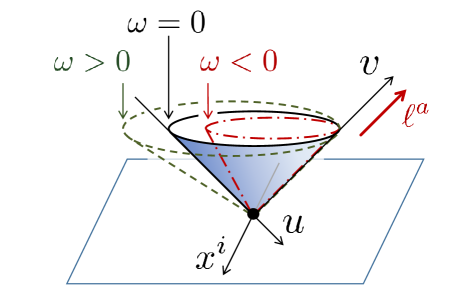
Figure 1: A schematic of characteristic cones for waves on the plane wave solution at $F(u,x,y)=0$, where $-u$ and $v$ are taken toward the future direction. The null cone with respect to the physical metric (72) is given by solid black line, and the characteristic cones obtained from the effective metrics (106) are shown by green dashed curve and red dot-dashed curve for $\omega>0$ and $\omega<0$, respectively. All the cones are aligned in the direction parallel to $\ell^{a}$ and they split in other directions if $\omega\neq 0$, hence the characteristic surfaces form a nested set of cones in general. The $u$-axis is aligned to the physical null cone since $F=0$ in this figure, while it is not the case when $F\neq 0$.

As long as $\omega$ in Eqs. (104) and (105) are finite, propagation speeds of waves are finite and we can define causality as usual despite the propagation becomes superluminal if $\omega>0$. The only difference from GR is that the causality is not defined with respect to the light cone but to the largest cone, which is realized for the largest $\omega$. Since the effective metrics (106) are always Lorentzian, the hyperbolicity of the field equation is maintained and the initial value problem is guaranteed to be well-posed. See Ref. Reall et al. (2014) for further discussions on the hyperbolicity in theories with modifications.

V Shock formation in shift-symmetric Horndeski theory

Based on the technique summarized in sections II and IV, we examine shock formation process in the Horndeski theory in this section. Some previous works Babichev (2016); Mukohyama et al. (2016); de Rham and Motohashi (2017) studied such shock (caustics) formation in generalized Galileon theories focusing on the simple wave solution of the scalar field. We re-examine the problem of shock formation taking the gravitational effect into account.

For this purpose, we focus on propagation of discontinuity in second derivatives of the scalar field and also the metric. Such a shock formation process based on transport of second-order discontinuity was studied in Reall et al. (2015) for Lovelock theories in higher dimensions, and it was found that gravitational wave in these theories suffers from shock formation generically. We will examine if this kind of phenomena could occur for gravitational wave in Horndeski theory, and also check what would happen for scalar field wave and shock formation in them when the gravitational sector is taken into account. For simplicity, we will focus on Horndeski theory with a single scalar field and particularly the shift-symmetric version of it, as we did in section IV.

We first review the formalism of shock formation for a generic equation of motion in section V.1, following Ref. Reall et al. (2015). We will apply this formalism to the shift-symmetric Horndeski theory in section V.2, and examine conditions to avoid the shock formation without specifying the background solution in section V.2.2.

To study properties of shock formation in this theory more explicitly, we focus on some examples of background solutions in the following sections. In section V.3, we take the plane wave solution studied in section IV as the background solution, and check if this solution suffers from the shock formation. Another typical class of solutions in the Horndeski theory is solutions whose two-dimensional angular part of the metric is maximally symmetric. For example, isotropic homogeneous cosmological solutions such as the FRW universe and also (dynamical) spherically-symmetric solutions belong to this class of solutions. We study shock formation on such dynamical solutions with two-dimensional maximally-symmetric part in their metrics in section V.4.

V.1 General formalism of shock formation

In this section, we introduce a formalism for propagation of discontinuity in second derivatives based on a general equation of motion (1). This formalism was introduced in Ref. Anile (2005) and was employed by Ref. Reall et al. (2015) to analyze shock formation process in Lovelock theories. We reproduce a part of the derivation explained therein to get our analysis oriented and to fix the notation.

We will employ the coordinates $(x^{a})=(x^{0},x^{\mu})$ introduced in section II.1, where a characteristic surface $\Sigma$ lies on $x^{0}=0$. We assume that the equation of motion has the following structure:

$$P_{IJ}(v_{,\mu\nu}\,,v_{,0}\,,v_{,\mu}\,,v\,,x)v_{J,00}+b_{I}(v_{,0\mu}\,,v_{,\mu\nu}\,,v_{,0}\,,v_{,\mu}\,,v\,,x)=0.$$ (108)

Here we assumed that $P_{IJ}$ is independent of $v_{,0\mu}$, which is the case in the shift-symmetric Horndeski theory at least. On the characteristic surface $\Sigma$, $\det P=0$ is satisfied and hence there are eigenvectors of $P$ with vanishing eigenvalues:

$$r_{I}P_{IJ}=P_{IJ}r_{J}=0,$$ (109)

where we assumed that $P_{IJ}$ is symmetric in its indices hence the left and right eigenvectors of $P$ coincide with each other.

Now let us consider time evolution from an initial time slice that intersects with $x^{0}=0$, and assume that the dynamical variable $v$ has a discontinuity in its second derivative with respect to $x^{0}$ at the locus of $x^{0}=0$ on the initial time slice. This discontinuity will propagate on $\Sigma$, and the solution on the past side of $\Sigma$ will not be influenced by the discontinuity. Hence we may regard wave of the discontinuity to propagate into the “background solution”, which is a solution to the unperturbed equation of motion (see Fig. 2).

Since the discontinuous part of (108) is given by $P_{IJ}\left[v_{J,00}\right]=0$, where a quantity in square brackets denotes its discontinuous part, comparing with Eq. (109) we find that $\left[v_{I,00}\right]$ must be proportional to an eigenvector $r_{I}$ and hence

$$\left[v_{I,00}\right]=\Pi(x^{\mu})\,r_{I},$$ (110)

where $\Pi(x^{i})$ is the proportional constant, which may be regarded as amplitude of the discontinuity.

In the following, we focus on how the amplitude of discontinuity $\Pi(x^{\mu})$ changes as it propagates on $\Sigma$. A transport equation of $\Pi$ can be constructed by firstly taking $x^{0}$ derivative of Eq. (108), acting $r^{I}$ on it to remove third derivatives with respect to $x^{0}$, and finally picking up discontinuous part of the resultant equation. Leaving the details of these steps to Ref. Reall et al. (2015), we find that the final outcome of these steps is given by

$${\cal K}^{\mu}\Pi_{,\mu}+{\cal M}\,\Pi+{\cal N}\,\Pi^{2}=0,$$ (111)

where

$${\cal K}^{\mu} =r_{I}r_{J}\frac{\partial b_{I}}{\partial v_{J,0\mu}}$$ (112)

$${\cal M} =r_{I}\biggl{\{}\frac{\partial b_{I}}{\partial v_{J,0\mu}}r_{J,\mu}+\left(\frac{\partial P_{IJ}}{\partial v_{K,\mu\nu}}v_{K,0\mu\nu}+\frac{\partial P_{IJ}}{\partial v_{K,\mu}}v_{K,0\mu}+\frac{\partial P_{IJ}}{\partial v_{K}}v_{K,0}+\frac{\partial P_{IJ}}{\partial x^{0}}+\frac{\partial b_{I}}{\partial v_{J,0}}\right)r_{J}+2\frac{\partial P_{IJ}}{\partial v_{K,0}}\left(v_{(J|,00}\right)^{-}r_{|K)}\biggr{\}}$$ (113)

$${\cal N} =r_{I}r_{J}r_{K}\frac{\partial P_{IJ}}{\partial v_{K,0}},$$ (114)

where $\left(v_{J,00}\right)^{-}\equiv\lim_{x^{0}\to-0}v_{J,00}$. The coefficients in Eq. (111) depend only on the field values at $x^{0}\to-0$, that is, the background solution on the past side of the characteristic surface. The discontinuity propagates along the integral curve generated by ${\cal K}^{\mu}$, which can be found by integrating

$$\frac{dx^{\mu}}{ds}={\cal K}^{\mu}(x^{\nu}),$$ (115)

where we have introduced a parameter $s$ along the integral curve $x^{\mu}=x^{\mu}(s)$ that becomes zero on the initial time slice. It can be shown that this integral curve coincides with a bicharacteristic curve, which is a geodesic curve with respect to the effective metric and along which waves on characteristic surface propagate Reall et al. (2015). Then, denoting $\dot{\Pi}\equiv d\Pi(s)/ds$, Eq. (111) may be written as

$$\dot{\Pi}+{\cal M}\,\Pi+{\cal N}\,\Pi^{2}=0.$$ (116)

An equation equivalent to Eq. (116) is obtained also for propagation of weakly nonlinear high frequency waves, whose frequency is sufficiently large compared to the background time dependence Choquet-Bruhat and Chrusciel (1969); Hunter and Keller (1983); Anile (2005); Choquet-Bruhat (2009); Reall et al. (2015). This equation is nonlinear in $\Pi$ as long as ${\cal N}$ does not vanish. In such a case, the theory is called genuinely nonlinear and suffers from shock formation as we see below. There are certain theories for which ${\cal N}$ identically vanishes and the above equation becomes linear, in which case the theory is called exceptional or linearly degenerate Anile (2005); Lax (1954); *Lax:1957hec; *1976pitm.book.....J; Boillat (1969). For example, GR coupled to a canonical scalar field is an exceptional theory.

Time evolution of the amplitude $\Pi(s)$ is described by the general solution of Eq. (116), which is given by

$$\Pi(s)=\frac{\Pi(0)e^{-\Phi(s)}}{1+\Pi(0)\int_{0}^{s}{\cal N}(s^{\prime})e^{-\Phi(s^{\prime})}ds^{\prime}}\,,$$ (117)

where

$$\Phi(s)\equiv\int_{0}^{s}{\cal M}(s^{\prime})ds^{\prime}.$$ (118)

When ${\cal N}=0$, $\Pi(s)$ obeying (117) diverges only when $\Phi(s)$ and hence ${\cal M}(s)$ do so. Since ${\cal M}(s)$ is determined only by information of the background solution and the characteristic surface on it, $\Phi$ diverges only when the background solution or $\Sigma$ is not regular. This happens when bicharacteristic curves on $\Sigma$ form a caustic on it by crossing with each other, where the amplitude of wave may diverge due to focusing effect. To distinguish it from the shock generated by nonlinear effect due to nonzero $\cal N$, sometimes this type of shock formation is called a linear shock Anile (2005).

When ${\cal N}\neq 0$, $\Pi(s)$ may diverge even when $\Phi(s)$ is regular, that is, there are no caustics on $\Sigma$. Such a divergence is realized when the denominator of (117) vanishes as $s$ increases from zero. As long as ${\cal N}(s)$ and $\Phi(s)$ are regular functions, we can always tune the signature and magnitude of $\Pi(0)$ to make $\Pi(0)\int_{0}^{s}{\cal N}(s^{\prime})e^{-\Phi(s^{\prime})}ds^{\prime}$ cross $-1$ at finite $s$, because there will be a sufficiently small region of $s$ in which $\int_{0}^{s}{\cal N}(s^{\prime})e^{-\Phi(s^{\prime})}ds^{\prime}$ behaves as a monotonic function of $s$. Hence, when ${\cal N}\neq 0$, it is guaranteed that $\Pi(s)$ can blow up if the initial amplitude $\Pi(0)$ is sufficiently large, where the divergence is expected to occur roughly at $s\sim-\bigl{(}\Pi(0)\,{\cal N}e^{-\Phi}\bigr{)}^{-1}$. In some cases, such a divergence of $\Pi(s)$ may happen even when $\Pi(0)$ is arbitrarily small, as we see an example in section V.3.

At the moment when $\Pi(s)$ diverges, second derivatives on the future side become infinite hence first derivatives become discontinuous at $\Sigma$. We call it a shock formation in this work. This phenomenon originates from the nonlinear effect due to nonzero ${\cal N}$ as we observed above, and also it can be seen that it occurs when two different characteristic surfaces collide with each other in time evolution Reall et al. (2015); Majda (1984); John and University ; Christodoulou (2007).

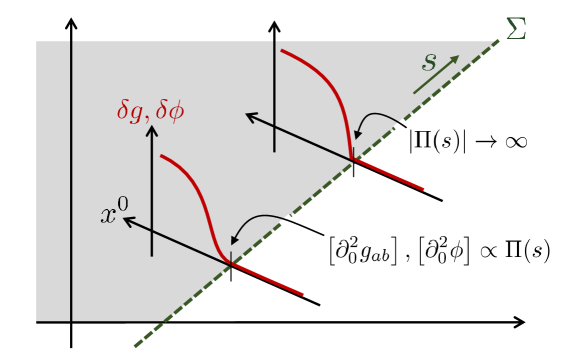
Figure 2: Propagation of discontinuity in second derivatives of the metric and scalar field, where red curves show profile of difference between the “background solution” without discontinuity and the solution to which the discontinuity is added. Solution in the future region of $\Sigma$ (shaded region) is influenced by the discontinuity, while that in the past region is not. The discontinuity propagates on $\Sigma$, and its amplitude $\Pi(s)$ evolves as it propagates along a bicharacteristic curve parameterized by $s$. When ${\cal N}\neq 0$, $\Pi(s)$ diverges at finite $s$ if the initial amplitude $\Pi(0)$ is chosen appropriately. At this point, second derivatives of fields blow up and single derivatives become discontinuous. We call this phenomenon a shock formation in this work.

V.2 Shock formation in shift-symmetric Horndeski theory

As shown in the previous section, shock formation in the discontinuity of second derivatives may occur when $\cal N$ defined by Eq. (114) does not vanish. In the following, we examine properties of $\cal N$ and shock formation process in the shift-symmetric Horndeski theory.

We first show the expression of $\cal N$ in the shift-symmetric Horndeski theory on general background in section V.2.1, then examine sufficient conditions for ${\cal N}=0$ in section V.2.2. To evaluate $\cal N$ explicitly, we need to specify the background solution. We do it for the plane wave solution in section V.3, and also for dynamical solution whose two-dimensional angular part of metric is maximally symmetric in section V.4.

V.2.1 Expression of $\cal N$ on general background

As shown in Eq. (114), the coefficient of the nonlinear term $\cal N$ is given by a derivative of the principal symbol of the field equation. In the shift-symmetric Horndeski theory, it is given by

$${\cal N}=\left(r_{ef}\frac{\partial}{\partial g_{ef,0}}+r_{\phi}\frac{\partial}{\partial\phi_{,0}}\right)\left\{\sum_{n=2}^{5}\bigl{(}\begin{array}[]{@{}cc@{}}r^{ab}&r_{\phi}\end{array}\bigr{)}\left({\begin{array}[]{@{}cc@{}}\frac{\partial{\cal G}^{n}_{ab}}{\partial g_{cd,00}}&\frac{\partial{\cal G}^{n}_{ab}}{\partial\phi_{,00}}\\ \frac{\partial\nabla^{h}{\cal J}_{h}^{n}}{\partial g_{cd,00}}&\frac{\partial\nabla^{h}{\cal J}_{h}^{n}}{\partial\phi_{,00}}\end{array}}\right)\left({\begin{array}[]{@{}c@{}}r_{cd}\\ r_{\phi}\end{array}}\right)\right\},$$ (124)

where we have taken $\xi_{a}=(dx^{0})_{a}$ and denoted $\xi_{c}\xi_{d}\frac{\partial}{\partial g_{ab,cd}}\equiv\frac{\partial}{\partial g_{ab,00}}$ and $\xi_{c}\xi_{d}\frac{\partial}{\partial\phi_{,cd}}\equiv\frac{\partial}{\partial\phi_{,00}}$. The derivatives with respect to $g_{ef,0}$ and $\phi_{,0}$ act only on the components of the two-by-two matrix. For the terms appearing in this expression, we can confirm that the following relation holds:

$$r_{ef}\frac{\partial}{\partial g_{ef,0}}\frac{\partial\nabla^{h}{\cal J}_{h}^{n}}{\partial\phi_{,00}} =\frac{\partial}{\partial\phi_{,0}}\frac{\partial{\cal G}^{n}_{ab}}{\partial\phi_{,00}}r^{ab}=\frac{\partial}{\partial\phi_{,0}}\frac{\partial\nabla^{h}{\cal J}_{h}^{n}}{\partial g_{cd,00}}r_{cd}\,,$$ (125)

$$r_{ef}\frac{\partial}{\partial g_{ef,0}}\frac{\partial{\cal G}^{n}_{ab}}{\partial\phi_{,00}}r^{ab} =r_{ef}\frac{\partial}{\partial g_{ef,0}}\frac{\partial\nabla^{h}{\cal J}_{h}^{n}}{\partial g_{cd,00}}r_{cd}=\frac{\partial}{\partial\phi_{,0}}\frac{\partial{\cal G}^{n}_{ab}}{\partial g_{cd,00}}r^{ab}r_{cd}\,.$$ (126)

Using them, $\cal N$ may be expressed as

$${\cal N}=\sum_{n=2}^{5}\biggl{\{}r^{ab}r_{cd}r_{ef}\frac{\partial}{\partial g_{ef}}\frac{\partial{\cal G}^{n}_{ab}}{\partial g_{cd,00}}+r_{\phi}{}^{3}\frac{\partial}{\partial\phi_{,0}}\frac{\partial\nabla^{h}{\cal J}^{n}_{h}}{\partial\phi_{,00}}+3\left(r_{\phi}r_{ef}\frac{\partial}{\partial g_{ef,0}}\frac{\partial{\cal G}^{n}_{ab}}{\partial\phi_{,00}}r^{ab}+r_{\phi}{}^{2}r_{ef}\frac{\partial}{\partial g_{ef,0}}\frac{\partial\nabla^{h}{\cal J}_{h}^{n}}{\partial\phi_{,00}}\right)\biggr{\}}.$$ (127)

We summarize explicit formula of the terms in (127) in appendix E. $\cal N$ on a general solution is given by a summation of the expressions therein. It does not vanish in general, hence we may expect that shock formation occurs generically in this theory, while there are some cases where ${\cal N}=0$ as we see below.

V.2.2 Sufficient conditions for ${\cal N}=0$

To evaluate $\cal N$ explicitly, we first need to specify the background solution, and then find characteristic surfaces and eigenvectors associated with them. We will follow such a procedure taking some examples of the background solutions later in sections V.3 and V.4. Before studying such examples, in this section let us examine sufficient conditions for $\cal N$ to vanish without specifying the background solution. Among various theories, we find that the k-essence Armendariz-Picon et al. (1999, 2001) coupled to GR stands out as a special theory where the scalar field decouples from metric sector, and that the scalar field version of the DBI model Born (1934); *Born425; *Dirac57 turns out to be the unique nontrivial theory to make ${\cal N}=0$ on the general background.

For the k-essence coupled to GR ($G_{3}=G_{5}=0$, $G_{4}=\text{{const.}}$ with general $K(X)$), non-vanishing parts of the (trace-reversed) principal symbol are given by

$$\xi_{s}\xi_{t}\frac{\partial\nabla^{\alpha}{\cal J}_{\alpha}^{2}}{\partial\phi_{,st}} =-K_{X}\left(g^{ab}-\frac{K_{XX}}{K_{X}}\phi^{|a}\phi^{|b}\right)\xi_{a}\xi_{b},$$ (128)

$$\xi_{s}\xi_{t}r_{qr}\frac{\partial\tilde{\cal G}^{4}{}_{a}^{b}}{\partial g_{qr,st}} =\frac{1}{2}G_{4}\left(\delta_{aa_{1}a_{2}}^{bb_{1}b_{2}}-\delta_{a}^{b}\delta_{a_{1}a_{2}}^{b_{1}b_{2}}\right)\xi^{a_{1}}\xi_{b_{1}}r^{a_{2}}_{b_{2}}=\frac{1}{2}G_{4}\left(-\xi^{2}r_{a}^{b}-r^{c}_{c}\xi_{a}\xi^{b}+\xi_{c}r^{c}_{a}\xi^{b}+\xi^{c}r_{c}^{b}\xi_{a}\right).$$ (129)

There are no terms that mix the scalar and metric parts, and in this sense the scalar part decouples from the metric part in this analysis. Characteristic surfaces can be found by equating these expressions with zero and solving for $\xi$.

In the metric part (129), if $\xi\neq 0$ we find that $r$ is forced to have a form $r_{ab}=\xi_{(a}X_{b)}$, which is pure gauge. Hence $\xi$ must be null to find physical modes, then Eq. (129) becomes a constraint which reduces the number of degree of freedom by four. Hence there will be two physical degrees of freedom in $r=(r_{ab},r_{\phi})=(r_{ab},0)$, which corresponds to the usual tensor modes in GR.

In the scalar part (128), the factor on the right-hand side gives an effective metric for the scalar mode as

$$\left(g^{ab}-\frac{K_{XX}}{K_{X}}\phi^{|a}\phi^{|b}\right)\xi_{a}\xi_{b}=0.$$ (130)

A surface whose normal vector $\xi$ satisfies this equation is characteristic, and the eigenvector is simply given by $r=(r_{ab},r_{\phi})=(0,r_{\phi})$.

Let us evaluate $\cal N$ for these modes next. For the k-essence coupled to GR, only (257) contributes among the terms appearing in $\cal N$, hence

$${\cal N}=r_{\phi}{}^{3}\frac{\partial}{\partial\phi_{,0}}\frac{\partial\nabla^{h}{\cal J}^{2}_{h}}{\partial\phi_{,00}}=3\phi^{|0}K_{XX}\xi^{2}-(\phi^{|0})^{3}K_{XXX},$$ (131)

where $\phi^{|0}=\xi_{a}\phi^{|a}$. For the tensor modes, this $\cal N$ vanishes identically and hence shock will not form. For the scalar mode, normalizing $r_{\phi}=1$ and using (130), we find

$${\cal N}=\frac{\left(\phi^{|0}\right)^{3}}{K_{X}}\left(3K_{XX}{}^{2}-K_{X}K_{XXX}\right).$$ (132)

The condition ${\cal N}=0$ to avoid shock formation is equivalent to $3K_{XX}{}^{2}-K_{X}K_{XXX}=0$ (assuming $\phi^{|0}\neq 0$), which may be viewed as a differential equation of $K(X)$. A trivial solution is $K\propto X$, which corresponds to a canonical scalar field. The general solution other than this one is given by

$$K=-\lambda\sqrt{c\pm X}+\Lambda,$$ (133)

where $\lambda,c,\Lambda$ are constants. This is the Lagrangian of the scalar DBI model, which reduces to the cuscuton model (${\cal L}\propto\sqrt{X}$) for $c=0$ or in the limit $X\to\infty$. Hence, among the theories described by the k-essence coupled to GR, the scalar DBI model (133) is singled out as the theory free from shock formation.

This behavior is the same as that of plane-symmetric simple wave solutions for probe scalar field studied by Ref. Babichev (2016); Mukohyama et al. (2016), where the scalar DBI model turned out to be the theory free from caustics formation. As discussed above, even in our setup the scalar and metric part decouples if $G_{3,5}(X)$ and non-constant part of $G_{4}(X)$ are set to zero. Having this decoupling, it seems natural that the result obtained from our setup coincides with those for the probe scalar field.

For the theories other than the k-essence coupled to GR, it seems difficult to find characteristics and eigenvectors since the scalar and metric parts do not decouple in the characteristic equation. However, there is a sufficient condition to realize ${\cal N}=0$ even in more general theories, which is to have $\phi^{|0}=\Gamma^{0}_{ab}=0$ on a characteristic surface. Imposing this condition to the expressions in appendix E, it can be checked that all the terms appearing in $\cal N$ vanish identically. A flat spacetime with constant $\phi$ is an example where this condition is satisfied, hence shock formation in the sense of section V.1 does not occur for wave propagating into such background. This is consistent with the results of Refs. Babichev (2016); Mukohyama et al. (2016); de Rham and Motohashi (2017) for simple waves of a probe scalar field, for which $\phi$ and its first derivative are not zero where caustics form. Another less trivial example of ${\cal N}=0$ is the Killing horizon with $\phi^{|0}=0$ imposed additionally, which was discussed in section III.2 in the context of the bi-Horndeski theory. On the Killing horizon $\Gamma^{0}_{ab}=0$ is satisfied by virtue of the condition (31), then $\cal N$ vanishes if $\phi^{|0}=0$ is satisfied as well.

V.3 Shock formation on plane wave solution

To study properties of shock formation for more complicated choices of $G_{n}(X)$ on generic background solutions, it seems that we need to look into explicit examples of background solutions and study wave propagation on them. Such a study using explicit background solutions is the main subject of this and the next sections.

The first example is the plane wave solution examined in section IV.2, where we follow the analysis of Ref. Reall et al. (2015) for shock formation on the plane wave solution in Lovelock theories. To prepare for the analysis, we introduce coordinates adapted to geodesics in this theory in section V.3.1. Using them, we examine shock formation on this solution in section V.3.2. We will find that the tensor modes or the gravitational wave, and also the scalar mode propagating along $\ell$ do not suffer from the shock formation, while the scalar mode propagating in the opposite direction forms a shock in general.

V.3.1 Geometry of characteristic surfaces

Characteristic surfaces on the plane wave background is given by null hypersurfaces with respect to effective metrics (106), which can be transformed as

$$G^{\omega}_{\mu\nu}dx^{\mu}dx^{\nu} =(F-\omega)du^{2}+2dudv+dx^{2}+dy^{2}=Fdu^{2}+2dudv^{\prime}+dx^{2}+dy^{2},$$ (134)

where we have introduced a new coordinate $v^{\prime}\equiv v-\frac{1}{2}\omega\,u$. For simplicity, we consider plane-fronted wave propagating from a surface $u=v^{\prime}=0$, and focus on the propagation in the (negative) $u$ direction, which is opposite from the direction along $\ell^{a}$ in Fig. 1. Such wave propagates along the null geodesics of the effective metric (134). Parameterizing the coordinates on a geodesic by affine parameter $\lambda$, the geodesic equation $\frac{d^{2}}{d\lambda^{2}}x^{a}+\Gamma^{a}_{bc}\frac{dx^{b}}{d\lambda}\frac{dx^{c}}{d\lambda}=0$ for the effective metric (134) is given by

$$\ddot{u}=0,\qquad\ddot{v}^{\prime}+\frac{1}{2}\dot{u}\left(\dot{u}F_{,u}+2\dot{x}^{\alpha}F_{,x^{\alpha}}\right)=0,\qquad\ddot{x}^{\alpha}-\frac{1}{2}\dot{u}\,F_{,x^{\alpha}}=0,$$ (135)

which are the $a=u,v^{\prime}$ and $x^{\alpha}(=x,y)$ components of the equation, respectively. The $u$ component implies that we may take $u=\lambda$. Below, we assume for simplicity that $\phi^{\prime}$ is a nonzero constant and $\phi^{\prime\prime}=0$. Also, we assume that $F(x^{\mu})$ is given by Eq. (79) whose homogeneous part is Eq. (80) with $a_{xx}=-a_{yy}=A$ and $a_{xy}=0$ for a constant $A$, that is,

$$F=-\frac{\kappa}{2}\phi^{\prime 2}\left(x^{2}+y^{2}\right)+A\,\left(x^{2}-y^{2}\right).$$ (136)

In this case, the $x^{\alpha}$ components of the geodesic equations can be solved by

$$x^{\alpha}=\eta^{\alpha}\cosh\bigl{(}\sqrt{A_{\alpha}}\lambda\bigr{)},$$ (137)

where $\eta^{I}$ is the initial position $x^{I}$ of a geodesic at $\lambda=0$, and $A_{\alpha}$ are given by

$$A_{x}=A-\frac{1}{4}\kappa\phi^{\prime 2},\qquad A_{y}=-A-\frac{1}{4}\kappa\phi^{\prime 2}.$$ (138)

Assuming $\kappa>0$, it is guaranteed that one of $A_{x}$ and $A_{y}$ becomes negative at least for any choice of $A$. The $v$ component can then be integrated as

$$v=-\frac{1}{4}\sum_{\alpha=x,y}\left(\eta^{\alpha}\right)^{2}\sinh\bigl{(}2\sqrt{A_{\alpha}}\lambda\bigr{)}.$$ (139)

Introducing Gaussian null coordinates adapted to the characteristic surface and geodesics

$$\eta^{\alpha}=\frac{x^{\alpha}}{\cosh\bigl{(}\sqrt{A_{\alpha}}\lambda\bigr{)}},\qquad x^{0}=v-\frac{1}{2}\omega\,u+\frac{1}{4}\sum_{\alpha=x,y}\sqrt{A_{\alpha}}\left(\eta^{\alpha}\right)^{2}\sinh\bigl{(}2\sqrt{A_{\alpha}}u\bigr{)},$$ (140)

the physical metric (72) becomes

$$ds^{2}=\omega du^{2}+2dudx^{0}+\sum_{\alpha=x,y}\cosh^{2}\bigl{(}\sqrt{A_{\alpha}}u\bigr{)}\left(d\eta^{\alpha}\right)^{2}.$$ (141)

The characteristic surface is at $x^{0}=0$ and its normal is given by $\xi=dx^{0}$. This metric becomes singular at $u=\pm\pi/2\sqrt{-A_{\alpha}}$ for $A_{\alpha}<0$, which corresponds to a caustic of the null geodesics. The only nonzero components of $\Gamma^{0}_{\alpha\beta}$ on $x^{0}=0$ are

$$\Gamma^{0}_{\alpha\alpha}=-\frac{1}{2}\sqrt{A_{\alpha}}\sinh\bigl{(}2\sqrt{A_{\alpha}}u\bigr{)}\qquad(\text{no sum on $\alpha$}).$$ (142)

This quantity is proportional to extrinsic curvature of the surface $x^{0}=0$ when it is not null.

V.3.2 $\cal N$ on the plane wave solution

$\cal N$ on the plane wave solution can be obtained by plugging the background solution (141), (142) with $\phi=\phi(u)$ into the general expression (127), whose explicit expressions are given in appendix E. We summarize the explicit formula obtained from this procedure in appendix F.

For the tensor mode (94), the only term that could contribute to $\cal N$ is the pure metric term (249), which is given by

$$r^{ab}r_{cd}r_{ef}\frac{\partial}{\partial g_{ef,0}}\frac{\partial{\cal G}^{5}_{ab}}{\partial g_{cd,00}}=\frac{\phi^{|0}}{4}XG_{5X}\delta_{aa_{1}a_{2}a_{3}}^{bb_{1}b_{2}b_{3}}\xi^{a}\xi_{b}r^{a_{1}}_{b_{1}}r^{a_{2}}_{b_{2}}r^{a_{3}}_{b_{3}}.$$ (143)

This term becomes zero because $X=0$ for the plane wave solution and also $\delta_{aa_{1}a_{2}a_{3}}^{bb_{1}b_{2}b_{3}}\xi^{a}\xi_{b}r^{a_{1}}_{b_{1}}r^{a_{2}}_{b_{2}}r^{a_{3}}_{b_{3}}$ vanishes identically if Eq. (94) is plugged in. Hence, $\cal N$ vanishes for the tensor modes on the plane wave background, or in other words gravitational wave on this background does not suffer from the shock formation.

For the scalar mode (95), $\cal N$ is given by

$${\cal N}=C_{+}\,t_{+}(u)+C_{-}\,t_{-}(u)+C_{0},$$ (144)

where

$$t_{\pm}(u)\equiv\sqrt{A_{x}}\tanh\bigl{(}\sqrt{A_{x}}u\bigr{)}\pm\sqrt{A_{y}}\tanh\bigl{(}\sqrt{A_{y}}u\bigr{)},$$ (145)

and $C_{\pm,0}$ are constants given by

$$C_{+} =\phi^{\prime 2}\left\{-\frac{1}{2G_{4}}\left(2G_{3X}G_{4X}+K_{X}G_{5X}\right)+\frac{2K_{XX}G_{3X}}{K_{X}}-G_{3XX}\right\}$$ (146)

$$C_{-} =-2A\,G_{5X}$$ (147)

$$C_{0} =\phi^{\prime 3}\left\{\frac{3}{G_{4}}\left(-G_{3X}{}^{2}-K_{X}G_{4XX}+K_{XX}G_{4X}\right)+\frac{3K_{XX}{}^{2}}{K_{X}}-K_{XXX}\right\}.$$ (148)

We have also taken a normalization $r_{\phi}=1$. This expression can be obtained following the calculation procedure explained above. Since we have already found geodesics and the coordinates adapted to it, as summarized in section V.3.1, there is an alternative method to derive $\cal N$ and also the entire part of the transport equation (111). In this method, we assume the field variables are given by

$$g_{ab}=\bar{g}_{ab}+\frac{1}{2}\,(x^{0})^{2}\,\Theta(x^{0})\,\Pi\bigl{(}u,\eta^{\alpha}\bigr{)}\,r_{ab}\,,\qquad\phi=\bar{\phi}+\frac{1}{2}\,(x^{0})^{2}\,\Theta(x^{0})\,\Pi\bigl{(}u,\eta^{\alpha}\bigr{)}\,r_{\phi}\,,$$ (149)

where $\bar{g}_{ab},\bar{\phi}$ are the background solutions and $\Theta(x^{0})$ is a step function. The above $g_{ab}$ and $\phi$ correctly give discontinuities in their second derivatives at $x^{0}=0$ as prescribed by Eq. (110). The transport equation (111) is obtained by evaluating the equation of motion at $x^{0}=0$ using Eq. (149), although it is not a correct solution in $x^{0}>0$.

With the aid of computer algebra, we can follow this alternative procedure to find the transport equation of $\Pi(u,\eta^{\alpha})$ to be given by

$${\cal K}\,\Pi_{,u}+{\cal M}\,\Pi+{\cal N}\,\Pi^{2}=0,$$ (150)

where $\cal N$ is given by Eq. (144), and the other coefficients turn out to be

$${\cal K}=-2K_{X},\qquad{\cal M}=-K_{X}t_{+}(u).$$ (151)

Then, the transport equation takes the form of Eq. (116) once the parameter $s$ along the bicharacteristic curve is introduced following (115) as

$$s=-\frac{1}{2K_{X}}\,u\,.$$ (152)

Now let us assume $A<0$ for definiteness, which implies $A_{x}<0$ and $|A_{x}|>|A_{y}|$. Then Eq. (145) becomes

$$t_{\pm}=\sqrt{-A_{x}}\tan\left(\frac{\pi}{2}\frac{s}{s_{*}}\right)\mp\sqrt{A_{y}}\tanh\left(\frac{\pi}{2}\frac{s}{s_{*}}\right),$$ (153)

where $s_{*}\equiv\frac{\pi}{4K_{X}\sqrt{-A_{x}}}$, and also $e^{-\Phi}$ appearing in the general solution of $\Pi(s)$ (117) is calculated as

$$e^{-\Phi}=\left\{\cos\left(\frac{\pi}{2}\frac{s}{s_{*}}\right)\cosh\left(2K_{X}\sqrt{A_{y}}s\right)\right\}^{-1/2}.$$ (154)

This quantity diverges for $s\to s_{*}-$ as $\propto(s_{*}-s)^{-1}$. Also, ${\cal N}e^{-\Phi}$ behaves for $s\to s_{*}-$ as

$${\cal N}e^{-\Phi}\simeq\frac{\left(C_{+}+C_{-}\right)\sqrt{-A_{x}}}{\cosh^{1/2}\left(\frac{\pi}{2}\sqrt{\frac{A_{y}}{-A_{x}}}\right)}\left(\frac{s_{*}-s}{s_{*}}\right)^{-3/2}\equiv{\cal N}_{0}\left(\frac{s_{*}-s}{s_{*}}\right)^{-3/2}.$$ (155)

This quantity diverges for $s\to s_{*}-$, hence the denominator of $\Pi(s)$ given by Eq. (117) can be zero at finite $s=s_{0}$ (such that $0<s_{0}<s_{*}$) no matter how small $|\Pi(0)|$ is. Hence, $\Pi(s)$ can diverge and the shock formation occurs at $s=s_{0}$ for an arbitrarily small $\Pi(0)$ in this example.

Assuming that ${\cal N}e^{-\Phi}$ is well approximated by Eq. (155), $s_{0}$ may be estimated as follows. Using Eq. (155) the integral in the denominator of (117) is estimated as

$$\int_{0}^{s}{\cal N}(s^{\prime})e^{-\Phi(s^{\prime})}ds^{\prime}\simeq 2s_{*}{\cal N}_{0}\left(\frac{s_{*}-s}{s_{*}}\right)^{-1/2}.$$ (156)

If this approximation is valid, $s_{0}$ will be approximated by

$$s_{0}\simeq\left\{1-\left(2\Pi(0)s_{*}{\cal N}_{0}\right)^{2}\right\}s_{*}.$$ (157)

The approximation used in Eq. (155) does not work if $C_{+}=C_{-}=0$. In this case, the denominator is given by $1+\Pi(0)C_{0}\int_{0}^{s}e^{-\Phi(s^{\prime})}ds^{\prime}$. The integral $\int_{0}^{s}e^{-\Phi(s^{\prime})}ds^{\prime}$ diverges at $s=s_{*}$, hence the denominator vanishes and $\Pi(s)$ diverges at $s<s_{*}$ if $\Pi(0)$ is taken so that $\Pi(0)C_{0}<0$. Hence the shock formation can occur even in this case.

In this example, $\Pi(0)$ diverges at $s=s_{*}$ even when $\cal N$ happens to vanish, because ${\cal N}=0$ implies $\Pi(s)=\Pi(0)e^{-\Phi}$ and $e^{-\Phi}\propto(s*-s)^{-1/2}\to\infty$ for $s\to s_{*}-$. This divergence occurs at the caustics of geodesics on $\Sigma$ and caused by the focusing effect in wave propagation.

Before closing this section, we briefly examine conditions to realize ${\cal N}=0$. If $K$ and $G_{n}$ satisfy

$$\begin{gathered}\frac{3}{G_{4}}\left(-G_{3X}{}^{2}-K_{X}G_{4XX}+K_{XX}G_{4X}\right)+\frac{3K_{XX}{}^{2}}{K_{X}}-K_{XXX}=0,\\ -\frac{1}{2G_{4}}\left(2G_{3X}G_{4X}+K_{X}G_{5X}\right)+\frac{2K_{XX}G_{3X}}{K_{X}}-G_{3XX}=0,\qquad A\,G_{5X}=0\end{gathered}$$ (158)

at $X=0$, $\cal N$ vanishes at any $u$ hence shock due to the nonlinear effect does not form. The scalar DBI model coupled to GR ($K=\lambda(1-\sqrt{1+c\,X}),G_{3}=G_{5}=0,G_{4}=\text{const.}$) and also the canonical scalar ($K\propto X,G_{3}=G_{5}=0$) with general $G_{4}(X)$ satisfy this condition, while it is not satisfied in more generic theories. For example, the pure Galileon coupled to GR

$$K=a_{2}X,\quad G_{3}=a_{3}X,\quad G_{4}=c+a_{4}X,\quad G_{5}=a_{5}X\qquad\left(a_{2}\neq 0,~{}c\neq 0\right)$$ (159)

does not satisfy (158) and makes $\cal N$ a nonzero function of $u$ unless $a_{3}=a_{5}\,A=0$. Also, the DBI Galileon

$$K=a_{2}(1-\sqrt{1+c\,X}),\quad G_{3}=a_{3}\log(1+c\,X),\quad G_{4}=a_{4}(1+c\,X)^{-1/2},\quad G_{5}=a_{5}(1+c\,X)^{-3/2}$$ (160)

with $a_{2},a_{4},c\neq 0$ does not satisfy (158) and it results in nonzero $\cal N$ given by

$${\cal N}=3c\,a_{5}\,A\,t_{-}(u)+c^{2}\left(\frac{a_{3}}{2}-\frac{3a_{2}a_{5}}{8a_{4}}\right)\phi^{\prime 2}t_{+}(u)+3c^{2}\left(\frac{c\,a_{2}}{4}-\frac{a_{3}{}^{2}}{a_{4}}\right)\phi^{\prime 3}.$$ (161)

V.4 Shock formation on two-dimensionally maximally-symmetric dynamical solutions

We now focus on another example of simple background solutions, in which spacetime is dynamical and has two-dimensional angular part that is maximally symmetric. Wave propagation on such solutions have been studied in Refs. Izumi (2014); Minamitsuji (2015) in the context of the Gauss-Bonnet gravity in higher dimensions and a scalar-tensor theory with a scalar field coupled to gravity non-minimally.

We first summarize basics of these solutions in section V.4.1. It turns out that gravitational wave on these solutions can be studied without specifying the background explicitly if the wave front is parallel to background symmetry direction. We summarize the results for such gravitational wave in section V.4.2. We will find that the gravitational wave is free from shock formation in this case, which is the same behavior as the gravitational wave on the plane wave background.

For the scalar field wave, we need more careful analysis as shown in section V.4.3. Based on the procedure in this section, we study homogeneous isotropic solutions, which we simply call the FRW universe in this work, in section V.4.4. We find that basic properties of the solution shown in Ref. Kobayashi et al. (2011), such as propagation speeds, are correctly reproduced from our analysis. Then we study properties of shock formation on this solution. Last, in section V.4.5 we look at another simple example, that is static spherically-symmetric solutions and waves with spherically-symmetric wave front on them. We will see that theories other than the scalar DBI model typically suffer from shock formation, even in the limit to treat the scalar field as a probe field on flat spacetime.

In section V.3 for the plane wave solution, we firstly clarified the structure of geodesics on a characteristic surface and then derived the full expression of the transport equation (150). Based on this expression, we gave an estimate (157) on the time parameter $s$ on the bicharacteristic curve at which the shock formation occurs. In the following sections, we skip deriving geodesics and the full expression of the transport equation, and evaluate only the coefficient of the nonlinear term ${\cal N}$ in the transport equation. As we argued based on the general solution of $\Pi(s)$ (117), it is guaranteed that shock formation occurs for sufficiently large $\Pi(0)$ when ${\cal N}$ is nonzero, assuming that ${\cal K}^{\mu}$ is a regular non-vanishing function and ${\cal M}$ is regular as well. To follow this argument, we need to know the expressions of all of ${\cal K}^{\mu}$, ${\cal M}$ and ${\cal N}$ in principle. However, without knowing the precise expressions of ${\cal K}^{\mu}$ and ${\cal M}$, we may still say that shock formation based on (117) does not occur if ${\cal N}$ identically vanishes, and also we may expect that shock would form if ${\cal N}\neq 0$ assuming ${\cal K}^{\mu}$ and ${\cal M}$ satisfies the above-mentioned properties. In the following, we take this attitude and check whether ${\cal N}$ vanishes or not, understanding that nonzero ${\cal N}$ suggests shock formation to occur while it is avoided when ${\cal N}=0$.

V.4.1 Two-dimensionally maximally-symmetric dynamical solutions

Solutions with metric whose two-dimensional spatial part is maximally symmetric can be expressed in general as

$$ds^{2} =f(\tau,\chi)\left(-d\tau^{2}+d\chi^{2}\right)+\rho^{2}(\tau,\chi)\gamma_{\alpha\beta}dx^{\alpha}dx^{\beta}\equiv f\eta_{AB}dx^{A}dx^{B}+\rho^{2}\gamma_{\alpha\beta}dx^{\alpha}dx^{\beta},$$ (162)

$$\phi =\phi(\tau,\chi),$$

where $x^{A}=\tau,\chi$ and $\gamma_{\alpha\beta}$ is the metric of the two-dimensional subspace with constant curvature $k=0,\pm 1$ spanned by $x^{\alpha}$. Non-vanishing components of the curvature tensor of this solution ares given by

$$R^{A_{1}A_{2}}_{B_{1}B_{2}}=\frac{\left(\partial_{\tau}^{2}-\partial_{\chi}^{2}\right)\log f}{2f}\delta^{A_{1}A_{2}}_{B_{1}B_{2}}\equiv R_{1}\delta^{A_{1}A_{2}}_{B_{1}B_{2}},\quad R^{A_{1}\alpha_{2}}_{B_{1}\beta_{2}}\equiv R_{2}{}^{A_{1}}_{B_{2}}\delta^{\alpha_{2}}_{\beta_{2}},\quad R^{\alpha_{1}\alpha_{2}}_{\beta_{1}\beta_{2}}=\frac{k\,f+\rho_{,\tau}^{2}-\rho_{,\chi}^{2}}{f\rho^{2}}\equiv R_{3}\delta^{\alpha_{1}\alpha_{2}}_{\beta_{1}\beta_{2}},$$ (163)

where

$$\left(R_{2}{}^{A}_{B}\right)=\frac{1}{2f^{2}\rho}\begin{pmatrix}-\left(f_{,\tau}\rho_{,\tau}+f_{,\chi}\rho_{,\chi}-2f\rho_{,\tau\tau}\right)&-2\left(f_{,(\tau}\rho_{,\chi)}-f\rho_{,\tau\chi}\right)\\ 2\left(f_{,(\tau}\rho_{,\chi)}-f\rho_{,\tau\chi}\right)&f_{,\tau}\rho_{,\tau}+f_{,\chi}\rho_{,\chi}-2f\rho_{,\chi\chi}\end{pmatrix}.$$ (164)

Also the nonzero components of $\phi_{|ab}$ are given by

$$\left(\phi_{|AB}\right)=-\frac{1}{2f}\begin{pmatrix}f_{,\tau}\phi_{,\tau}+f_{,\chi}\phi_{,\chi}-2f\phi_{,\tau\tau}&2\left(f_{,(\tau}\phi_{,\chi)}-f\phi_{,\tau\chi}\right)\\ 2\left(f_{,(\tau}\phi_{,\chi)}-f\phi_{,\tau\chi}\right)&f_{,\tau}\phi_{,\tau}+f_{,\chi}\phi_{,\chi}-2f\phi_{,\chi\chi}\end{pmatrix},\quad\phi_{|\alpha\beta}=\frac{\rho}{f}\left(-\rho_{,\tau}\phi_{,\tau}+\rho_{,\chi}\phi_{,\chi}\right)\gamma_{\alpha\beta}.$$ (165)

We can evaluate the principal symbol and the quantities appearing in $\cal N$ using these formula.

Below, we focus on wave whose wave front shares the same symmetry as background spacetime, that is, we assume that the wave front is given by a $\chi$-constant surface and $\xi_{\mu}$ has only $(\tau,\chi)$ components. For example, plane wave in flat FRW universe and wave with spherically-symmetric wave front around a spherically-symmetric dynamical star fulfill such an assumption.

This assumption enable us to work out the characteristic analysis for the tensor modes without specifying explicit form of the background solution, and it is the main target in section V.4.2. For the scalar mode, to simplify the analysis summarized in section V.4.3, we will consider two explicit examples of background solutions that satisfy the above assumption. The first one is plane wave propagating on homogeneous isotropic solutions (Fig. 3), and the second one is wave with spherically-symmetric wave front on spherically-symmetric static background solutions (Fig. 3), which are studied in sections V.4.4 and V.4.5, respectively.

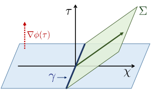
(a) FRW universe

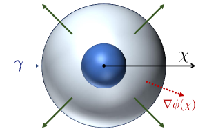
(b) Spherically-symmetric static solution

Figure 3: Examples of two-dimensionally maximally-symmetric dynamical solutions and wave propagation therein. Panel 3 shows a flat FRW universe and wave with plane-symmetric wave front, and panel 3 shows a spherically-symmetric static background solution and wave with spherically-symmetric wave front. Gradient of the background scalar field is aligned to the symmetry direction of the background spacetime in these examples, while they may point toward different directions at the level of the general ansatz (162).

V.4.2 Gravitational wave

Characteristic surfaces on the background (162) can be found by solving the eigenvalue equation (68) following the procedure of section IV.1. To accomplish it for gravitational wave, we focus on a vector given by

$$r=(r_{ab},r_{\phi})=(r^{\text{(T)}}_{ab},0),$$ (166)

where $r^{\text{(T)}}_{ab}$ is a traceless tensor which has components only in the angular directions, that is, $r^{\text{(T)}}_{AB}=0$. By explicit calculations, we can check that this vector is actually an eigenvector of $\tilde{\cal R}$ as follows. The scalar and mixed parts of $\tilde{\cal R}$ vanish for this vector, hence only the metric part shown in appendix D.2 remains nontrivial and is given by

$$\xi_{s}\xi_{t}r^{\text{(T)}}_{qr}\frac{\partial\tilde{\cal G}^{4}{}_{a}^{b}}{\partial g_{qr,st}}=\frac{1}{2}G_{4X}\,\delta^{B_{1}B_{2}}_{A_{1}A_{2}}\xi^{A_{1}}\xi_{B_{1}}\phi^{|A_{2}}\phi_{|B_{2}}\,r^{\text{(T)}}{}^{b}_{a},\quad\xi_{s}\xi_{t}r^{\text{(T)}}_{qr}\frac{\partial\tilde{\cal G}^{5}{}_{a}^{b}}{\partial g_{qr,st}}=-\frac{1}{2}XG_{5X}\,\delta^{B_{1}B_{2}}_{A_{1}A_{2}}\xi^{A_{1}}\xi_{B_{1}}\phi^{|A_{2}}_{|B_{2}}\,r^{\text{(T)}}{}^{b}_{a},$$ (167)

hence we have $\tilde{\cal R}\cdot r=\lambda\,r$ with

$$\lambda=\frac{1}{G_{4}-2XG_{4X}}\delta^{B_{1}B_{2}}_{A_{1}A_{2}}\xi^{A_{1}}\xi_{B_{1}}\left(G_{4X}\phi^{|A_{2}}\phi_{|B_{2}}-XG_{5X}\phi^{|A_{2}}_{|B_{2}}\right).$$ (168)

From this expression, we find that characteristics are determined by

$$\left\{\left(G_{4}-2XG_{4X}\right)\delta^{B}_{A}-\delta^{BB_{1}}_{AA_{1}}\left(G_{4X}\phi^{|A_{1}}\phi_{|B_{1}}-XG_{5X}\phi^{|A_{1}}_{|B_{1}}\right)\right\}\xi^{A}\xi_{B}=0,$$ (169)

where the expression in the curly brackets is the effective metric for gravitational wave on the background (162).

Propagation speed of the gravitational wave can be read out from the effective metric (169). When the background solution is homogeneous and isotropic, the propagation speed $c_{T}=|\xi_{\tau}/\xi_{\chi}|$ in the frame for which $\phi=\phi(\tau)$ coincides with that shown in Kobayashi et al. (2011), which is given by $c_{T}=\sqrt{{\cal F}_{T}/{\cal G}_{T}}$ with

$${\cal F}_{T}\equiv 2\bigl{(}G_{4}-X\ddot{\phi}G_{5X}\bigr{)},\qquad{\cal G}_{T}\equiv 2\bigl{(}G_{4}-2XG_{4X}-HX\dot{\phi}G_{5X}\bigr{)}.$$ (170)

Let us check if shock formation could occur for gravitational wave (166) by evaluating the coefficient $\cal N$ in the discontinuity transport equation. The only term that could be nonzero is $r^{ab}r_{cd}r_{ef}\frac{\partial}{\partial g_{ef,0}}\frac{\partial{\cal G}^{5}_{ab}}{\partial g_{cd,00}}$ given by Eq. (249), which is proportional to $\delta_{aa_{1}a_{2}a_{3}}^{bb_{1}b_{2}b_{3}}\xi^{a}\xi_{b}{r^{\text{(T)}}}^{a_{1}}_{b_{1}}{r^{\text{(T)}}}^{a_{2}}_{b_{2}}{r^{\text{(T)}}}^{a_{3}}_{b_{3}}$. However, $r^{\text{(T)}}$ is a traceless tensor living in the two-dimensional angular part of the spacetime and then Eq. (249), which involves three $r^{\text{(T)}}$ tensors contracted with a single generalized Kronecker delta, identically vanishes. Hence $\cal N$ is zero and shock formation does not occur for gravitational wave on the background (162).

V.4.3 Scalar field wave

Next, we study wave that involves the scalar field and examine if it suffers from shock formation. Recent studies about a probe scalar field on flat background clarified that shock generically forms in the Horndeski theory while it is avoided in the DBI-Galileon theory Babichev (2016); Mukohyama et al. (2016); de Rham and Motohashi (2017). We re-examine these results using our formalism for transport of discontinuity in second derivatives of fields.

The first step is to find a characteristic surface and an eigenmode corresponding to scalar field wave. On the background (162) and for wave that inherits the symmetry of the background, we may assume the eigenvector $r$ has a structure given by

$$r=(r_{ab},r_{\phi}),\qquad r_{AB}=r_{\eta}\,\eta_{AB}+\frac{2r_{\gamma}}{\xi^{2}}\xi_{A}\xi_{B},\quad r_{A\alpha}=0,\quad r_{\alpha\beta}=r_{\gamma}\,\gamma_{\alpha\beta},$$ (171)

where $r_{\phi}$, $r_{\eta}$ and $r_{\gamma}$ are functions of $\tau,\chi$. The term involving $\xi_{A}\xi_{B}$ is the gauge part added so that $r$ satisfies the transverse condition (63).

For the ansatz (171), we may parameterize the eigenvector by $(r_{\eta},r_{\gamma},r_{\phi})$, and then the eigenvalue equation (68) should have three eigenvalues in general. Plugging the ansatz (171) into (68), we can confirm that two eigenvalues are proportional to $\xi^{2}$ and another one is a nontrivial function of $\xi$. This nontrivial eigenvalue corresponds to a physical scalar mode propagating on the characteristic surface, and the propagation speed is given in terms of $\xi$ as $c_{S}=|\xi_{\tau}/\xi_{\chi}|$.

Expression of the nontrivial eigenvalue and eigenvector are generically lengthy and not illuminating. There are some cases in which their expressions become simple and $\cal N$ can be calculated explicitly. We examine such cases realized for simple background solutions below.

V.4.4 Shock formation in FRW universe

Based on the ansatz (162), a solution describing homogeneous and isotropic universe is realized by

$$f=\rho^{2}=a(\tau)^{2},\quad\phi=\phi(\tau),$$ (172)

where $\tau$ in this case is the conformal time from which a standard time coordinate may be defined by $dt=a(\tau)d\tau$. We will use the Hubble parameter in terms of $t$, $H(t)\equiv a_{,t}/a$, and also the notation $\dot{\phi}\equiv\phi_{,t}$ and $X=\dot{\phi}^{2}/2$ below. $tt$ and $\chi\chi$ components of the background equation of motion (44) give the modified Friedmann equations

$$-K+2XK_{X}+6HX\dot{\phi}G_{3X}-6H^{2}\left(G_{4}-4XG_{4X}+4X^{2}G_{4XX}\right)+2H^{3}X\dot{\phi}\left(5G_{5X}+2XG_{5XX}\right)=0,$$ (173)

$${\cal E}\equiv K+2\bigl{(}3H^{2}+2\dot{H}\bigr{)}\left(G_{4}-2XG_{4X}\right)-4H\bigl{(}H^{2}+\dot{H}\bigr{)}X\dot{\phi}G_{5X}\\ -2\ddot{\phi}\left[XG_{3X}+2H\dot{\phi}\left(G_{4X}+2XG_{4XX}\right)+H^{2}X\left(3G_{5X}+2XG_{5XX}\right)\right]=0.$$ (174)

Properties of the background solution (172) and its perturbations are studied by Ref. Kobayashi et al. (2011). Particularly, propagation speed of the scalar mode is given by $c_{S}=\sqrt{{\cal F}_{S}/{\cal G}_{S}}$, where

$$\Sigma\equiv X{\cal E}_{,X}+\frac{1}{2}H{\cal E}_{,H},\quad\Theta\equiv-\frac{1}{6}{\cal E}_{,H},\quad{\cal F}_{S}\equiv\frac{1}{a}\frac{d}{dt}\left(\frac{a}{\Theta}{\cal G}_{T}^{2}\right)-{\cal F}_{T},\quad{\cal G}_{S}\equiv\frac{\Sigma}{\Theta^{2}}{\cal G}_{T}^{2}+3{\cal G}_{T}.$$ (175)

This $c_{S}$ coincides with the propagation speed obtained from the eigenvalue obtained above once the Friedmann equations (173), (174) are imposed.

Expressions of the propagation speed and the eigenvector $r$ become lengthy in general. One exception is the case discussed in section V.2.2, where $G_{3,4,5}$ are constants while $K(X)$ is kept general. In this case it follows that

$$(r_{ab},r_{\phi})=(0,r_{\phi}),\qquad c_{S}^{2}=\frac{K_{X}}{K_{X}+2XK_{XX}},$$ (176)

and also we can check that ${\cal N}=0$ is achieved by the scalar DBI model coupled to GR, as we have seen in section V.2.2.

For general $K(X)$ and $G_{n}(X)$, the propagation speed and the eigenvector takes more complicated form. A case that gives relatively simple $c_{S}$ and $r$ is when

$$K=-\lambda\sqrt{1+c\,X},\quad G_{4}=a_{4}\sqrt{1+\tilde{c}\,X},\quad G_{3,5}=0,$$ (177)

where $\lambda,c,a_{4},\tilde{c}$ are constants that satisfies $c\neq\tilde{c}$. In this case, using the Friedmann equations (173), (174) we can simplify the propagation speed and the eigenvector as

$$c_{S}{}^{2}=1+c\,X,\qquad\left(r_{\eta},r_{\gamma},r_{\phi}\right)\propto\left(\frac{\tilde{c}\left(1+c\,X\right)^{3/4}}{c\,\dot{\phi}},\frac{\tilde{c}\,\dot{\phi}}{\left(1+c\,X\right)^{1/4}},\sqrt{\frac{6a_{4}}{\lambda}}\left(1+\tilde{c}\,X\right)^{1/4}\right),$$ (178)

and we can check that $\cal N$ identically vanishes in this case. Other choices of $G_{4}$ such as $G_{4}\propto\left(1+X\right)^{-1/2}$ typically result in ${\cal N}\neq 0$. Hence, it seems that the choice (177) is special among other choices of $K(X)$ and $G_{4}(X)$ in the sense that it leads to a cosmological solution free from shock formation.

For other choices of $K(X)$ and $G_{n}(X)$, $\cal N$ becomes nonzero generically. For example, a choice given by $K=G_{5}=0$ with constant $G_{4}$ and general $G_{3}(X)$ results in

$$c_{S}{}^{2}=\frac{G_{3X}\left(23G_{3X}+16XG_{3XX}\right)}{3\left(5G_{3X}+4XG_{3XX}\right)^{2}},\quad\left(r_{\eta},r_{\gamma},r_{\phi}\right)\propto\Bigl{(}\left(c_{S}{}^{2}+1\right)G_{3X},\left(c_{S}{}^{2}-1\right)XG_{3X},\left(c_{S}{}^{2}-1\right)G_{4}\Bigr{)}.$$ (179)

where Eqs. (173) and (174) are used to simplify the expressions. Using them, $\cal N$ is calculated as

$${\cal N}\propto\dot{\phi}X\Bigl{[}-55G_{3X}{}^{3}-120X^{3}G_{3XX}{}^{3}+4X^{2}G_{3X}G_{3XX}\left(-55G_{3XX}+14XG_{3XXX}\right)\\ +2XG_{3X}{}^{2}\left(-59G_{3XX}+38XG_{3XXX}\right)\Bigr{]}.$$ (180)

For a generic choice of $G_{3}$, this expression does not vanish unless $\dot{\phi}=0$ and hence shock would form. In principle, we can find $G_{3}(X)$ that realizes ${\cal N}=0$ by equating Eq. (180) with zero and solving it as an ODE for $G_{3}(X)$. It seems difficult to obtain a closed form of $G_{3}(X)$ obtained in this way. Also it can be confirmed that $\cal N$ does not vanish for some simple choices such as $G_{3}\propto\log(1+c\,X)$ and $(1+c\,X)^{n}$ with integer $n$.

V.4.5 Shock formation on spherically-symmetric static solutions

Another example of a simple solution described by (162) is a spherically-symmetric static solution

$$f=f(\chi),\quad\rho=\rho(\chi),\quad\phi=\phi(\chi),$$ (181)

where $\gamma_{\alpha\beta}$ is taken as the metric on $S^{2}$ with unit radius. The metric functions and the scalar field in Eq. 181 are fixed by integrating $tt$ and $\theta\theta$ components of the metric equation (44) and the scalar equation (49) regarding them as second-order ODEs on $f(\chi)$, $\rho(\chi)$ and $\phi(\chi)$. The $rr$ component of the metric equation is given by $f,\rho,\phi$ and their first derivatives, and it can be regarded as a constraint on the variables. Below, we use the above second-order equations of motion to eliminate second derivatives of background fields from various expressions.

An eigenvector can be parameterized as (171) even in this case. Also, as argued in section V.2.2, the k-essence coupled with GR is an example for which various quantities are easily derived. In this case, the eigenvector is given by $(r_{\eta},r_{\gamma},r_{\phi})\propto(0,0,1)$, and the propagation speed is given by

$$c_{S}{}^{2}=\frac{K_{X}+2XK_{XX}}{K_{X}},$$ (182)

which is the reciprocal of the propagation speed in the FRW universe Armendariz-Picon and Lim (2005). $\cal N$ in this case is given by (132), and the scalar DBI model turns out to be the unique theory other than the canonical scalar field that makes $\cal N$ vanishing.

$\cal N$ does not vanish for a generic choice of $G_{n}(X)$, as it was the case of the FRW universe background. In that case, there was a nontrivial example (177) that realizes ${\cal N}=0$. Let us check if the shock formation could occur for this choice (177) when the background is spherically symmetric and static. In this case, using the background equations we can show that

$$c_{S}{}^{2} =\frac{1}{1+c\,X},\qquad\left(r_{\eta},r_{\gamma},r_{\phi}\right)\propto\left(\tilde{r}_{\eta},-2c\tilde{c}a_{4}\phi^{\prime}X\sqrt{1+\tilde{c}\,X}\rho^{\prime 2},2ca_{4}X\left(1+\tilde{c}\,X\right)^{3/2}f\rho\rho^{\prime}\right),$$ (183)

$$\frac{\tilde{r}_{\eta}}{\tilde{c}\,\phi^{\prime}} \equiv f(1+c\,X)^{1/2}(1+\tilde{c}\,X)^{3/2}\left(\lambda\sqrt{1+\tilde{c}\,X}\rho^{2}-2a_{4}\sqrt{1+c\,X}\right)-2a_{4}(1+c\,X)\sqrt{1+\tilde{c}\,X}\rho^{\prime 2}.$$

We can check that propagation speeds of the modes propagating in the positive and negative $r$ directions coincide with each other. Using these expressions we can confirm that $\cal N$ does not vanish in this case. Hence, the theory with (177) suffers from shock formation on a spherically-symmetric static background realized within this theory, contrarily to the case of the FRW universe background. Other choices such as $K=G_{5}=0$ with constant $G_{4}$ and generic $G_{3}$ give nonzero $\cal N$.

We can also check what happens when the scalar field is treated as a probe field and its gravitational backreaction is neglected. In this case, the background spacetime becomes flat ($f=1,\rho=\chi$), and the background scalar field is determined by the scalar equation (49). The principal symbol and $\cal N$ are given by their pure scalar part evaluated with a flat metric, and using these expressions we can find a characteristic surface and check if shock formation could occur on it. For the k-essence model, the propagation speed is given by (182) and ${\cal N}=0$ is realized only for the scalar DBI model. For other models in which only one of the arbitrary functions $G_{3,4}(X)$ is non-zero, propagation speeds are given by

$$\text{pure $G_{3}$ model}: \quad c_{S}^{2}=\frac{4}{3}\frac{G_{3X}+XG_{3XX}}{G_{3X}}$$ (184)

$$\text{pure $G_{4}$ model}: \quad c_{S}^{2}=\frac{3G_{4XX}+2XG_{4XXX}}{3G_{4XX}}.$$ (185)

In the pure $G_{5}$ model, the scalar field equation becomes trivial for any static configuration of $\phi(\chi)$. Hence, a discontinuity in second derivative added at the initial time can remain static unlikely to the other cases where such a discontinuity propagates at finite speed. In the pure $G_{3}$ theory, $\cal N$ does not vanish for a generic choice of the arbitrary function $G_{3}(X)$. We can still find some exceptions for which $\cal N$ vanishes on nontrivial backgrounds, such as $G_{4}\propto\sqrt{c+X}$ and $G_{4}\propto(1+X)^{2}$, where the former corresponds to the example (177) in which the metric part of the theory is taken into account.

VI Summary and discussion

In this paper, we studied properties of wave propagation and causality defined by it, and also of the shock formation process in scalar-tensor theories. For these studies we especially focused on the Horndeski theory, which is the most general scalar-tensor theory with one scalar field whose Euler-Lagrange equation is up to second order in derivatives, and its generalization with two scalar fields developed in Ohashi et al. (2015), which we called the bi-Horndeski theory in this work. The latter theory reduces to the former and also to the generalized multi-Galileon theory by setting the arbitrary functions appropriately, as shown in appendix B.

About the wave propagation, in section II we showed that characteristic surfaces in the bi-Horndeski theory are not null in general, that is, propagation speeds of gravitational wave and scalar field wave can be faster or slower than the light speed defined by physical metric. We also showed that a Killing horizon in this theory is not a causal edge in general, hence there may be superluminal modes that can propagate across a Killing horizon. However, it turned out that such propagation across a Killing horizon is prohibited if the scalar fields share the Killing symmetry on the horizon. These properties may be regarded as natural generalizations of those found for scalar-tensor theories with a non-minimally coupled scalar field studied in Ref. Minamitsuji (2015). In Barausse et al. (2011) the causal structure in Einstein-aether and Hořava–Lifshitz theories were studied, and it was noticed that the universal horizon, which acts as the causal edge for any mode, is orthogonal to the background vector field in those theories. This property seems similar to that found in this work if the gradient of the background scalar field is identified as such a vector field. It would be interesting to examine this possible correspondence and its implications.

We also studied wave propagation and causal structure on a nontrivial background taking the plane wave solution constructed by Ref. Babichev (2012) as an example. This exact solution has a null direction to which waves of metric and scalar field propagate. We found that the causal cones for metric and scalar perturbations on this background form a nested set of cones that are aligned along the background null direction, as shown in Fig. 2 of section IV. As long as a the background solution is regular, there will be a characteristic cone with the largest but finite opening, which will define the causality on this background solution.

In section V, we focused on another phenomenon associated with wave propagation, that is, the shock formation caused by nonlinear self interaction of waves. For this purpose, we generalized the formalism of Reall et al. (2015) for the transport of discontinuity in second derivatives of the metric in Lovelock theories to the Horndeski theory with shift symmetry in the scalar field. It turned out that the k-essence coupled to GR can be studied without specifying the background solution using this formalism, and the results are summarized in section V.2.2. For this class of theory, we found that shock may form for scalar field wave while not for gravitational wave. We have also shown that, Among the theories described by the k-essence, the scalar DBI model besides the canonical scalar field turned out to be the unique nontrivial theory that is free from shock formation. Such a property was found by previous works Babichev (2016); Mukohyama et al. (2016); de Rham and Motohashi (2017); Boillat et al. (2006); *1959PThPS...9...69T; *Whitham_chap17; *Barbashov:1966frq; *doi:10.1142/9789812708908_0003; *Deser:1998wv for simple waves of a probe scalar field on flat spacetime. Our result implies that this property persists even on nontrivial background that involves non-vanishing scalar field and spacetime curvature.

To study properties of the shock formation on various backgrounds, we focused on the plane wave solution and also dynamical solutions in which two-dimensional angular part of the spacetime is maximally symmetric in sections V.3 and V.4, respectively. On the plane wave background studied in section V.3, we found that shock formation does not occur for wave propagating in the background null direction, while it occurs for the scalar field wave propagating in the opposite direction. The gravitational wave, however, does not suffer from shock formation even when it is propagating in this direction. On the two-dimensionally maximally-symmetric dynamical solutions, we studied waves whose wave front is aligned to the background symmetry direction in section V.4. It turned out that shock formation occurs for scalar field wave in general, while it does not for gravitational wave. Taking some typical background solutions such as the FRW solutions and spherically-symmetric static solutions, we examined conditions for shock formation. We found that theories other than the scalar DBI model generically suffer from shock formation on these backgrounds.

In any example studied in this work, the propagation modes corresponding to gravitational wave were always free from shock formation. If this feature persists on any background solution, we may conclude that the gravitational wave in this class of theory is more well-behaved compared to the scalar field, which typically suffers from shock formation. On the other hand, if we could find some background solutions or nontrivial shape of wavefront for which shock formation occurs even for gravitational wave, it might give interesting implications to gravitational wave observations which was realized recently Abbott et al. (2016). Such studies on shock formation in gravitational wave with nontrivial wave front on nontrivial background would be one possible future extension of this work.

There are some other open issues and future directions related to this work. First one is about the time evolution after shock formation. When a shock forms, the derivatives of fields diverge there and the theory would break down unless higher-order corrections to the theory ameliorate the singular behavior, or unless we accept such a field configuration as a weak solution of the theory. Also, a shock formation would correspond to a naked singularity formation unless it is covered by an event horizon or resolved by corrections to the theory, as argued in Reall et al. (2015); Mukohyama et al. (2016). It would be interesting to study time evolution after shock formation by taking higher-order corrections into account or by regarding a shock as a weak solution. Next one is about extending the analysis in this work to more general theories. In this work we used the shift-symmetric Horndeski theory for a single scalar field in the analysis of shock formation just for simplicity, although it is desirable to conduct the study using more broader class of theories. It would be fruitful to extend the shock formation analysis, and also the analysis on wave propagation, for the bi-Horndeski theory and other more general theories mentioned in section I. Last, the phenomena discussed in this work could be important in time evolution that involves nonlinear dynamics of gravity and scalar fields. Investigations on wave propagation and shock formation in scalar-tensor theories with such nonlinear dynamics might provide useful implications in the context of cosmology and astrophysics.

Appendix A Field equation of the most general bi-scalar-tensor theory

In this appendix, we present the equations of motion for the most general bi-scalar-tensor theory. See Ref. Ohashi et al. (2015) for more details.

A.1 Gravitational field equations

The gravitational field equations for the most general bi-scalar-tensor theory are given by

$$\mathcal{G}{}^{a}_{b} =A\delta^{a}_{b}+\left(-2\mathcal{F}_{,I,J}-4\mathcal{W}_{,I,J}+A_{,IJ}+2D_{IKJ,L}X^{KL}-16E_{KIMNJ,L}X^{KL}X^{MN}-16J_{K[I,L],J}X^{KL}\right)\phi^{(I|a}\phi^{J)}_{|b}$$

$$+\left[-2\mathcal{F}_{,I}-4\mathcal{W}_{,I}+2\left(D_{JKI}+8J_{J[K,I]}\right)X^{JK}-8E_{JKLMI}X^{JK}X^{LM}\right]\delta^{ac}_{bd}\phi^{I|d}_{|c}$$

$$+D_{IJK}\delta^{ace}_{bdf}\phi^{I}_{|c}\phi^{J|d}\phi^{K|f}_{|e}+E_{IJKLM}\delta^{aceg}_{bdfh}\phi^{I}_{|c}\phi^{J|d}\phi^{K}_{|e}\phi^{L|f}\phi^{M|h}_{|g}+\left(\frac{1}{2}\mathcal{F}+\mathcal{W}\right)\delta^{ace}_{bdf}R_{ce}^{~{}~{}\,df}+\mathcal{F}_{,IJ}\delta^{ace}_{bdf}\phi^{I|d}_{|c}\phi^{J|f}_{|e}$$

$$+J_{IJ}\delta^{aceg}_{bdfh}\phi^{I}_{|c}\phi^{J|d}R_{eg}^{~{}~{}\,fh}+2J_{IJ,KL}\delta^{aceg}_{bdfh}\phi^{I}_{|c}\phi^{J|d}\phi^{K|f}_{|e}\phi^{L|h}_{|g}+K_{I}\delta^{aceg}_{bdfh}\phi^{I|d}_{|c}R_{eg}^{~{}~{}\,fh}+\frac{2}{3}K_{I,JK}\delta^{aceg}_{bdfh}\phi^{I|d}_{|c}\phi^{J|f}_{|e}\phi^{K|h}_{|g},$$ (186)

where $A,D_{IJK},E_{IJKLM},J_{IJ},K_{I}$ are arbitrary functions of $\phi^{I}$ and $X^{IJ}$, $\mathcal{W}$ are arbitrary function of $\phi$. These functions are subject to

$$D_{IJK}=D_{JIK},\qquad E_{IJKLM}=-E_{KJILM}=-E_{ILKJM}=E_{JILKM},\qquad J_{IJ}=J_{JI},$$ (187)

and $\mathcal{F}$ is defined as

$$\mathcal{F}=\int dX^{IJ}\left(2J_{IJ}-2K_{I,J}+J_{KI,JL}X^{KL}\right).$$ (188)

A.2 Scalar field equations

The scalar field equations for the most general bi-scalar-tensor theory are given by

$${\cal E}_{I}=2{\cal Q}_{I}+\delta^{cegl}_{bdhm}\left(-\gamma_{JIKL}\phi^{K|b}\phi^{J}_{|c}\phi^{L|d}_{|e}R_{gl}^{~{}~{}\,hm}+\frac{2}{3}\sigma_{JIKLMN}\phi^{J}_{|c}\phi^{M|b}\phi^{K|d}_{|e}\phi^{L|h}_{|g}\phi^{N|m}_{|l}\right),$$ (189)

where

$$\gamma_{IJKL}=-2J_{IJ,KL}+H_{IKJL},\qquad\sigma_{IJKLMN}=H_{IJKL,MN}-H_{IMNL,JK}.$$ (190)

The explicit form of ${\cal Q}_{I}$ is given by

$${\cal Q}_{I}\equiv{\cal Q}_{I}^{(A)}+{\cal Q}_{I}^{(B)}+{\cal Q}_{I}^{(C)}+{\cal Q}_{I}^{(D)}+{\cal Q}_{I}^{(E)}+{\cal Q}_{I}^{(G)}+{\cal Q}_{I}^{(H)}+{\cal Q}_{I}^{(I)}+{\cal Q}_{I}^{(J)}+{\cal Q}_{I}^{(K)}+{\cal Q}_{I}^{(L)},$$ (191)

where

$$\mathcal{Q}_{I}^{(A)} =A_{,I},$$ (192)

$$\mathcal{Q}_{I}^{(B)} =-2B_{IJ,K}X^{JK}-B_{IJ,KL}\phi^{K}_{|c}\phi^{L}{}^{|cb}\phi^{J}_{|b}+B_{IJ}\phi^{J}_{|b}{}^{|b},$$ (193)

$$\mathcal{Q}_{I}^{(C)} =C_{J,I}\phi^{J}_{|c}{}^{|c},$$ (194)

$$\mathcal{Q}_{I}^{(D)} =D_{JKL,I}\delta^{ce}_{df}\phi^{J}_{|c}\phi^{K}{}^{|d}\phi^{L}_{|e}{}^{|f}+2D_{IJK,L}X^{JL}\phi^{K}_{|c}{}^{|c}+D_{IJK,L}\phi^{J}{}^{|c}\phi^{K}_{|cd}\phi^{L}{}^{|d}$$

$$\quad+D_{IJK,LM}\delta^{ce}_{bf}\phi^{L}_{|d}\phi^{M}{}^{|db}\phi^{J}_{|c}\phi^{K}_{|e}{}^{|f}-D_{IJK}\delta^{ce}_{bf}\phi^{J}_{|c}{}^{|b}\phi^{K}_{|e}{}^{|f}-\frac{1}{2}D_{IJK}\delta^{ce}_{bf}\phi^{J}_{|c}\phi^{K}{}^{|l}R_{el}^{~{}~{}\,bf},$$ (195)

$$\mathcal{Q}_{I}^{(E)} =E_{JKLMN,I}\delta^{ceg}_{dfh}\phi^{J}_{|c}\phi^{K}{}^{|d}\phi^{L}_{|e}\phi^{M}{}^{|f}\phi^{N}_{|g}{}^{|h}-2E_{LJKIM,N}\delta^{ceg}_{dfh}\phi^{L}_{|c}\phi^{J}{}^{|d}\phi^{K}_{|e}\phi^{N}{}^{|f}\phi^{M}_{|g}{}^{|h}$$

$$\quad-2E_{LJKIM,NO}\delta^{ceg}_{bfh}\phi^{N}_{|l}\phi^{O}{}{}^{|lb}\phi^{L}_{|c}\phi^{K}_{|e}\phi^{J}{}^{|f}\phi^{M}_{|g}{}^{|h}+4E_{LJKIM}\delta^{ceg}_{bfh}\phi^{L}_{|c}{}^{|b}\phi^{K}_{|e}\phi^{J}{}^{|f}\phi^{M}_{|g}{}^{|h}$$

$$\quad+E_{LJKIM}\delta^{ceg}_{bfh}\phi^{L}_{|c}\phi^{K}_{|e}\phi^{J}{}^{|f}\phi^{M}{}^{|l}R_{gl}^{~{}\,bh},$$ (196)

$$\mathcal{Q}_{I}^{(G)} =G_{JK,I}\delta^{ce}_{df}\phi^{J}_{|c}{}^{|d}\phi^{K}_{|e}{}^{|f},$$ (197)

$$\mathcal{Q}_{I}^{(H)} =H_{JKLM,I}\delta^{ceg}_{dfh}\phi^{J}_{|c}\phi^{K}{}^{|d}\phi^{L}_{|e}{}^{|f}\phi^{M}_{|g}{}^{|h}+2H_{IJKL,M}X^{JM}\delta^{eg}_{fh}\phi^{K}_{|e}{}^{|f}\phi^{L}_{|g}{}^{|h}+2H_{IJKL,M}\delta^{cg}_{fh}\phi^{J}_{|c}\phi^{M}{}^{|e}\phi^{K}_{|e}{}^{|f}\phi^{L}_{|g}{}^{|h}$$

$$\quad-H_{IJKL}\delta^{ceg}_{bfh}\phi^{J}_{|c}{}^{|b}\phi^{K}_{|e}{}^{|f}\phi^{L}_{|g}{}^{|h}-H_{IJKL}\delta^{ceg}_{bfh}\phi^{J}_{|c}\phi^{K}_{|e}{}^{|f}\phi^{L}{}^{|l}R_{gl}^{~{}~{}\,bh}+H_{IJKL,MN}\delta^{ceg}_{bfh}\phi^{M}_{|l}\phi^{N}{}^{|lb}\phi^{J}_{|c}\phi^{K}_{|e}{}^{|f}\phi^{L}_{|g}{}^{|h},$$ (198)

$$\mathcal{Q}_{I}^{(I)} =I_{,I}\delta^{ce}_{df}R_{ce}^{~{}~{}\,df},$$ (199)

$$\mathcal{Q}_{I}^{(J)} =J_{JK,I}\delta^{ceg}_{dfh}\phi^{J}_{|c}\phi^{K}{}^{|d}R_{eg}^{~{}~{}\,fh}+2J_{IJ,K}X^{JK}\delta^{eg}_{fh}R_{eg}^{~{}~{}\,fh}+2J_{IJ,K}\delta^{cg}_{fh}\phi^{J}_{|c}\phi^{K}{}^{|e}R_{eg}^{~{}~{}\,fh}$$

$$\quad+J_{IJ,KL}\delta^{ceg}_{bfh}\phi^{K}_{|d}\phi^{L}{}^{|db}\phi^{J}_{|c}R_{eg}^{~{}~{}\,fh}-J_{IJ}\delta^{ceg}_{bfh}\phi^{J}_{|c}{}^{|b}R_{eg}^{~{}~{}\,fh},$$ (200)

$$\mathcal{Q}_{I}^{(K)} =K_{J,I}\delta^{ceg}_{dfh}\phi^{J}_{|c}{}^{|d}R_{eg}^{~{}~{}\,fh}-\frac{1}{2}K_{J,IK}\delta^{cegl}_{dfhm}\phi^{K}_{|c}{}^{|d}\phi^{J}_{|e}{}^{|f}R_{gl}^{~{}~{}\,hm}-\frac{1}{8}K_{I}\delta_{dfhm}^{cegl}R_{ce}^{~{}~{}\,df}R_{gl}^{~{}~{}\,hm},$$ (201)

$$\mathcal{Q}_{I}^{(L)} =L_{JKL,I}\delta^{ceg}_{dfh}\phi^{J}_{|c}{}^{|d}\phi^{K}_{|e}{}^{|f}\phi^{L}_{|g}{}^{|h}-\frac{1}{4}L_{LJK,IM}\delta^{cegl}_{dfhm}\phi^{M}_{|c}{}^{|d}\phi^{L}_{|e}{}^{|f}\phi^{J}_{|g}{}^{|h}\phi^{K}_{|l}{}^{|m},$$ (202)

and the coefficient functions appearing in ${\cal Q}_{I}$ are defined as

$$B_{IJ} =-2\left(\mathcal{F}+2\mathcal{W}\right)_{,I,J}+A_{,IJ}+2D_{(I|K|J),L}X^{KL}-16E_{K(I|MN|J),L}X^{KL}X^{MN}-8\left(J_{K(I,J),L}-J_{KL,I,J}\right)X^{KL},$$ (203)

$$C_{I} =-2\left(\mathcal{F}+2\mathcal{W}\right)_{,I}+2\left(D_{JKI}+8J_{J[K,I]}\right)X^{JK}-8E_{JKLMI}X^{JK}X^{LM},$$ (204)

$$G_{IJ} =2J_{IJ}-2K_{(I,J)}+4J_{K(I,J)L}X^{KL},$$ (205)

$$H_{IJKL} =2J_{IJ,KL},$$ (206)

$$K_{[I,J]} =-2J_{K[I,J]L}X^{KL},$$ (207)

$$K_{I,JK} =K_{J,IK},$$ (208)

$$L_{IJK} =\frac{2}{3}K_{(I,JK)},$$ (209)

$$I =\frac{1}{2}\mathcal{F}+\mathcal{W}.$$ (210)

Appendix B Bi-scalar-tensor theory to generalized multi-Galileon and Horndeski theory

In this section, we show explicitly the relationship of the most general bi-scalar-tensor theory with the generalized multi-Galileon theory and Horndeski theory.

B.1 Generalized multi-Galileon theory

The Lagrangian of the generalized multi-Galileon theory is given as

$$\frac{1}{\sqrt{-g}}\mathcal{L} =G_{2}-G_{3}{}_{I}\phi_{I}{}_{|a}^{|a}+G_{4}R+G_{4}{}_{,IJ}\left(\phi^{I|a}_{|a}\phi^{J|b}_{|b}-\phi^{I}_{|ab}\phi^{J|ab}\right)$$

$$\quad+G_{5I}G^{ab}\phi^{I}_{|ab}-\frac{1}{6}G_{5I,JK}\left(\phi^{I|a}_{|a}\phi^{J|b}_{|b}\phi^{K|c}_{|c}-3\phi^{I|a}_{|a}\phi^{J|c}_{|b}\phi^{K|b}_{|c}+2\phi^{I|b}_{|a}\phi^{J|c}_{|b}\phi^{K|a}_{|c}\right),$$ (211)

where $G_{2},G_{3}{}_{I},G_{4}$ and $G_{5}{}_{I}$ are arbitrary functions of $\phi^{I}$ and $X^{IJ}$, and $G^{ab}$ is the Einstein tensor. The functions $G_{3}{}_{I}{}_{,JK},G_{4}{}_{,IJ,KL},G_{5}{}_{I,JK}$ and $G_{5}{}_{I,JK,LM}$ must be totally symmetric in all of their indices, $I,J,K,L$ and $M$ in order for the field equations to be of second order.

We can move from the the most general bi-scalar-tensor theory to the generalized multi-Galileon theory by setting the functions as (see Ref. Ohashi et al. (2015) for details)

$$A =-\frac{1}{2}G_{2}+G_{3(I,J)}X^{IJ}-2G_{4,I,J}X^{IJ},\quad D_{IJK}=0,\quad E_{IJKLM}=0,$$ (212)

$$J_{IJ} =\frac{1}{4}\left(G_{4IJ}-G_{5(I,J)}\right),\quad K_{I}=-\frac{1}{4}X^{JK}G_{5IJK}.$$

B.2 Horndeski theory

The Lagrangian of the Horndeski theory is written as

$$\frac{1}{\sqrt{-g}}\mathcal{L}=G_{2}-G_{3}{}\phi{}_{|a}^{|a}+G_{4}R+G_{4}{}_{,X}\left(\phi^{|a}_{|a}\phi^{|b}_{|b}-\phi_{|ab}\phi^{|ab}\right)+G_{5}G^{ab}\phi_{|ab}-\frac{G_{5,X}}{6}\left(\phi^{|a}_{|a}\phi^{|b}_{|b}\phi^{|c}_{|c}-3\phi^{|a}_{|a}\phi^{|c}_{|b}\phi^{|b}_{|c}+2\phi^{|b}_{|a}\phi^{|c}_{|b}\phi^{|a}_{|c}\right),$$ (213)

We can move from the the most general bi-scalar-tensor theory to the Horndeski theory by setting the functions as

$$\phi^{I} \rightarrow\phi,\quad A\rightarrow-\frac{1}{2}G_{2}+G_{3,\phi}X-2G_{4,\phi\phi}X,\quad D_{IJK}\rightarrow 0,\quad E_{IJKLM}\rightarrow 0,$$ (214)

$$J_{IJ} \rightarrow\frac{1}{4}\left(G_{4,X}-G_{5,\phi}\right),\quad K_{I}\rightarrow-\frac{1}{4}XG_{5,X}.$$

Appendix C Integrability conditions for equations of motion

As we discussed in section II.2 and also in Ohashi et al. (2015), we need to impose integrability conditions to the equations of motion of the bi-Horndeski theory summarized in appendix A, in order to guarantee the existence of Lagrangian that gives these equations of motion. The integrability conditions are summarized as

$$\frac{\delta E^{ab}(x)}{\delta g_{cd}(y)}-\frac{\delta E^{cd}(y)}{\delta g_{ab}(x)}=0,\qquad\frac{\delta E^{ab}(x)}{\delta\phi_{I}(y)}-\frac{\delta E_{I}(y)}{\delta g_{ab}(x)}=0,\qquad\frac{\delta E_{I}(x)}{\delta\phi_{J}(y)}-\frac{\delta E_{J}(y)}{\delta\phi_{I}(x)}=0,$$ (215)

where the equations of motion of the bi-Horndeski theory have the structure

$$E^{ab}=E^{ab}\bigl{(}g_{cd}\,,g_{cd,e}\,,g_{cd,ef}\,,\phi_{I}\,,\phi_{I,c}\,,\phi_{I,cd}\bigr{)},\qquad E_{I}=E_{I}\bigl{(}g_{cd}\,,g_{cd,e}\,,g_{cd,ef}\,,\phi_{J}\,,\phi_{J,c}\,,\phi_{J,cd}\bigr{)}.$$ (216)

Applying the method of Deffayet et al. (2014) to these equations, we can derive the integrability conditions as

$$E^{ab;cd,ef}-E^{cd;ab,ef}=0$$ (217)

$$E^{ab;cd,e}+E^{cd;ab,e}-2\partial_{f}E^{cd;ab,ef}=0$$ (218)

$$E^{ab;cd}-E^{cd;ab}+\partial_{e}\left(E^{cd;ab,e}-\partial_{f}E^{cd;ab,ef}\right)=0$$ (219)

$$E_{I}{}^{;ab}_{J}-E_{J}{}^{;ab}_{I}=0$$ (220)

$$E_{I}{}^{;a}_{J}+E_{J}{}^{;a}_{I}-2\partial_{b}E_{J}{}^{;ab}_{I}=0$$ (221)

$$E_{I,J}-E_{J,I}+\partial_{a}\left(E_{J}{}^{;a}_{I}-\partial_{b}E_{J}{}^{;ab}_{I}\right)=0$$ (222)

$$E^{ab}{}_{I}^{;cd}-E_{I}{}^{;ab,cd}=0$$ (223)

$$E^{ab}{}_{I}^{;c}+E_{I}{}^{;ab,c}-2\partial_{d}E_{I}{}^{;ab,cd}=0$$ (224)

$$E^{ab}{}_{,I}-E_{I}{}^{;ab}+\partial_{c}\left(E_{I}{}^{;ab,c}-\partial_{d}E_{I}{}^{;ab,cd}\right)=0,$$ (225)

where

$$E^{ab;cd,ef}\equiv\frac{\partial E^{ab}}{\partial g_{cd,ef}},\quad E^{ab;cd,e}\equiv\frac{\partial E^{ab}}{\partial g_{cd,e}},\quad E^{ab;cd}\equiv\frac{\partial E^{ab}}{\partial g_{cd}},\quad E_{I}{}^{;ab}_{J}\equiv\frac{\partial E_{I}}{\partial\phi_{J,ab}},\quad E_{I}{}^{;a}_{J}\equiv\frac{\partial E_{I}}{\partial\phi_{J,a}},\quad E_{I}{}_{,J}\equiv\frac{\partial E_{I}}{\partial\phi_{J}},$$ (226)

$$E^{ab}{}_{,I}\equiv\frac{\partial E^{ab}}{\partial\phi_{I}},\quad E_{I}{}^{;ab}\equiv\frac{\partial E_{I}}{\partial g_{ab}},\quad E^{ab}{}_{I}^{;c}\equiv\frac{\partial E^{ab}}{\partial\phi_{I,c}},\quad E_{I}{}^{;ab,c}\equiv\frac{\partial E_{I}}{\partial g_{ab,c}},\quad E^{ab}{}_{I}^{;cd}\equiv\frac{\partial E^{ab}}{\partial\phi_{I,cd}},\quad E_{I}{}^{;ab,cd}\equiv\frac{\partial E_{I}}{\partial g_{ab,cd}}.$$

The condition (217) is a part of the so-called invariance identity following from covariance of the theory, and has already been imposed on the equations of motion of the bi-Horndeski theory in Ohashi et al. (2015). The other equations above have not been imposed yet, and would give constraints to the arbitrary functions of the theory.

Appendix D Principal symbol of shift-symmetric Horndeski theory

In this appendix, we summarize the explicit formula of the principal symbol (55), which is obtained by taking derivatives of the field equations (44), (49) of the shift-symmetric Horndeski theory. Since we have the symmetry (57), below we show only $\xi_{s}\xi_{t}r^{ab}\frac{\partial{\cal G}_{ab}^{n}}{\partial\phi_{,st}}$, which is equal to $r_{qr}\xi_{s}\xi_{t}\frac{\partial\nabla^{a}{\cal J}_{a}^{n}}{\partial g_{qr,st}}$. To derive the principal symbol, we use

$$R_{abcd}=-2g_{[a|[c,d]|b]}+\cdots,\qquad\frac{\partial R_{a_{1}a_{2}}^{b_{1}b_{2}}}{\partial g_{qr,st}}r_{qr}\xi_{s}\xi_{t}=-2r_{[a_{1}}^{[b_{1}}\xi_{a_{2}]}\xi^{b_{2}]}.$$ (227)

D.1 Principal symbol

The metric part of the principal symbol is given by

$$\xi_{s}\xi_{t}r^{ab}r_{qr}\frac{\partial{\cal G}^{2}_{ab}}{\partial g_{qr,st}} =\xi_{s}\xi_{t}r^{ab}r_{qr}\frac{\partial{\cal G}^{3}_{ab}}{\partial g_{qr,st}}=0$$ (228)

$$\xi_{s}\xi_{t}r^{ab}r_{qr}\frac{\partial{\cal G}^{4}_{ab}}{\partial g_{qr,st}} =\frac{1}{2}\left(G_{4}-2XG_{4X}\right)\delta_{aa_{1}a_{2}}^{bb_{1}b_{2}}\xi^{a}\xi_{b}r^{a_{1}}_{b_{1}}r^{a_{2}}_{b_{2}}-\frac{1}{2}G_{4X}\delta_{aa_{1}a_{2}a_{3}}^{bb_{1}b_{2}b_{3}}\xi^{a}\xi_{b}r^{a_{1}}_{b_{1}}r^{a_{2}}_{b_{2}}\phi^{|a_{3}}\phi_{|b_{3}}$$ (229)

$$\xi_{s}\xi_{t}r^{ab}r_{qr}\frac{\partial{\cal G}^{5}_{ab}}{\partial g_{qr,st}} =\frac{1}{2}XG_{5X}\delta_{aa_{1}a_{2}a_{3}}^{bb_{1}b_{2}b_{3}}\xi^{a}\xi_{b}r^{a_{1}}_{b_{1}}r^{a_{2}}_{b_{2}}\phi^{|a_{3}}_{|b_{3}}.$$ (230)

The mixed part between the metric and scalar parts is given by

$$\xi_{\mu}\xi_{\nu}r^{ab}\frac{\partial{\cal G}^{2}_{ab}}{\partial\phi_{,st}} =0$$ (231)

$$\xi_{s}\xi_{t}r^{ab}\frac{\partial{\cal G}^{3}_{ab}}{\partial\phi_{,st}} =-\frac{1}{2}G_{3X}\left(\delta_{aa_{1}a_{2}}^{bb_{1}b_{2}}\xi^{a}\xi_{b}r_{a_{1}}^{b_{1}}\phi^{|a_{2}}\phi_{|b_{2}}+2X\delta_{bb_{1}}^{aa_{1}}\xi^{a}\xi_{b}r^{a_{2}}_{b_{2}}\right)$$ (232)

$$\xi_{s}\xi_{t}r^{ab}\frac{\partial{\cal G}^{4}_{ab}}{\partial\phi_{,st}} =\left(G_{4X}+2XG_{4XX}\right)\delta_{aa_{1}a_{2}}^{bb_{1}b_{2}}\xi^{a}\xi_{b}r^{a_{1}}_{b_{1}}\phi^{|a_{2}}_{|b_{2}}+G_{4XX}\delta_{aa_{1}a_{2}a_{3}}^{bb_{1}b_{2}b_{3}}\xi^{a}\xi_{b}r^{a_{1}}_{b_{1}}\phi^{|a_{2}}_{|b_{2}}\phi^{|a_{3}}\phi_{|b_{3}}$$ (233)

$$\xi_{s}\xi_{t}r^{ab}\frac{\partial{\cal G}^{5}_{ab}}{\partial\phi_{,st}} =-\frac{1}{2}\left(G_{5X}+XG_{5XX}\right)\delta_{aa_{1}a_{2}a_{3}}^{bb_{1}b_{2}b_{3}}\xi^{a}\xi_{b}r^{a_{1}}_{b_{1}}\phi^{|a_{2}}_{|b_{2}}\phi^{|a_{3}}_{|b_{3}}-\frac{1}{4}XG_{5X}\delta_{aa_{1}a_{2}a_{3}}^{bb_{1}b_{2}b_{3}}\xi^{a}\xi_{b}r^{a_{1}}_{b_{1}}R^{a_{2}a_{3}}_{b_{2}b_{3}}.$$ (234)

Finally the scalar part is given by (where $\xi^{2}\equiv\xi_{a}\xi^{a}$ and $\xi\cdot\phi\equiv\xi_{a}\phi^{|a}$)

$$\xi_{s}\xi_{t}\frac{\partial\nabla^{a}{\cal J}_{a}^{2}}{\partial\phi_{,st}} =-K_{X}\xi^{2}+K_{XX}(\xi\cdot\phi)^{2}$$ (235)

$$\xi_{s}\xi_{t}\frac{\partial\nabla^{a}{\cal J}_{a}^{3}}{\partial\phi_{,st}} =2\left(G_{3X}+XG_{3XX}\right)\delta_{aa_{1}}^{bb_{1}}\xi^{a}\xi_{b}\phi^{|a_{1}}_{|b_{1}}+G_{3XX}\delta_{aa_{1}a_{2}}^{bb_{1}b_{2}}\xi^{a}\xi_{b}\phi^{|a_{1}}_{|b_{1}}\phi^{|a_{2}}\phi_{|b_{2}}$$ (236)

$$\xi_{s}\xi_{t}\frac{\partial\nabla^{a}{\cal J}_{a}^{4}}{\partial\phi_{,st}} =-\left(3G_{4XX}+2XG_{4XXX}\right)\delta_{aa_{1}a_{2}}^{bb_{1}b_{2}}\xi^{a}\xi_{b}\phi^{|a_{1}}_{|b_{1}}\phi^{|a_{2}}_{|b_{2}}-G_{4XXX}\delta_{aa_{1}a_{2}a_{3}}^{bb_{1}b_{2}b_{3}}\xi^{a}\xi_{b}\phi^{|a_{1}}_{|b_{1}}\phi^{|a_{2}}_{|b_{2}}\phi^{|a_{3}}\phi_{|b_{3}}$$

$$\quad-\frac{1}{2}\left(G_{4X}+2XG_{4XX}\right)\delta_{aa_{1}a_{2}}^{bb_{1}b_{2}}\xi^{a}\xi_{b}R^{a_{1}a_{2}}_{b_{1}b_{2}}-\frac{1}{2}G_{4XX}\delta_{aa_{1}a_{2}a_{3}}^{bb_{1}b_{2}b_{3}}\xi^{a}\xi_{b}R^{a_{1}a_{2}}_{b_{1}b_{2}}\phi^{|a_{3}}\phi_{|b_{3}}$$ (237)

$$\xi_{s}\xi_{t}\frac{\partial\nabla^{a}{\cal J}_{a}^{5}}{\partial\phi_{,st}} =\frac{2G_{5XX}+XG_{5XXX}}{3}\delta_{aa_{1}a_{2}a_{3}}^{bb_{1}b_{2}b_{3}}\xi^{a}\xi_{b}\phi^{|a_{1}}_{|b_{1}}\phi^{|a_{2}}_{|b_{2}}\phi^{|a_{3}}_{|b_{3}}+\frac{G_{5X}+XG_{5XX}}{2}\delta_{aa_{1}a_{2}a_{3}}^{bb_{1}b_{2}b_{3}}\xi^{a}\xi_{b}\phi^{|a_{1}}_{|b_{1}}R^{a_{2}a_{3}}_{b_{2}b_{3}}.$$ (238)

Expressions with non-contracted indices is obtained just by removing one of $r^{a}_{b}$ from the expressions above.

D.2 Trace-reversed principal symbol

For the analysis in sections IV and V, we need also the trace-reversed expressions of the principal symbol defined by

$$\tilde{P}=P-\frac{1}{2}\left({\mathrm{t}r}P\right)g.$$ (239)

We summarize its expression below. Since the scalar part of it is the same as the above expressions, we show only the metric part. The pure metric part is given by

$$\xi_{s}\xi_{t}r_{qr}\frac{\partial\tilde{\cal G}^{2}{}_{a}^{b}}{\partial g_{qr,st}} =\xi_{s}\xi_{t}r_{qr}\frac{\partial\tilde{\cal G}^{3}{}_{a}^{b}}{\partial g_{qr,st}}=0$$ (240)

$$\xi_{s}\xi_{t}r_{qr}\frac{\partial\tilde{\cal G}^{4}{}_{a}^{b}}{\partial g_{qr,st}} =\frac{G_{4}-2XG_{4X}}{2}\left(\delta_{aa_{1}a_{2}}^{bb_{1}b_{2}}-\delta_{a}^{b}\delta_{a_{1}a_{2}}^{b_{1}b_{2}}\right)\xi^{a_{1}}\xi_{b_{1}}r^{a_{2}}_{b_{2}}-\frac{G_{4X}}{2}\left(\delta_{aa_{1}a_{2}a_{3}}^{bb_{1}b_{2}b_{3}}-\frac{1}{2}\delta_{a}^{b}\delta_{a_{1}a_{2}a_{3}}^{b_{1}b_{2}b_{3}}\right)\xi^{a_{1}}\xi_{b_{1}}r^{a_{2}}_{b_{2}}\phi^{|a_{3}}\phi_{|b_{3}}$$ (241)

$$\xi_{s}\xi_{t}r_{qr}\frac{\partial\tilde{\cal G}^{5}{}_{a}^{b}}{\partial g_{qr,st}} =\frac{1}{2}XG_{5X}\left(\delta_{aa_{1}a_{2}a_{3}}^{bb_{1}b_{2}b_{3}}-\frac{1}{2}\delta_{a}^{b}\delta_{a_{1}a_{2}a_{3}}^{b_{1}b_{2}b_{3}}\right)\xi^{a_{1}}\xi_{b_{1}}r^{a_{2}}_{b_{2}}\phi^{|a_{3}}_{|b_{3}},$$ (242)

and the mixed part between the metric and scalar parts is given by

$$\xi_{s}\xi_{t}\frac{\partial\tilde{\cal G}^{2}{}_{a}^{b}}{\partial\phi_{,st}} =0$$ (243)

$$\xi_{s}\xi_{t}\frac{\partial\tilde{\cal G}^{3}{}_{a}^{b}}{\partial\phi_{,st}} =-\frac{1}{2}G_{3X}\left\{\left(\delta_{aa_{1}a_{2}}^{bb_{1}b_{2}}-\delta_{a}^{b}\delta_{a_{1}a_{2}}^{b_{1}b_{2}}\right)\xi^{a_{1}}\xi_{b_{1}}\phi^{|a_{2}}\phi_{|b_{2}}+X\left(2\delta_{aa_{1}}^{bb_{1}}\xi^{a_{1}}\xi_{b_{1}}-3\xi^{2}\delta_{a}^{b}\right)\right\}$$ (244)

$$\xi_{s}\xi_{t}\frac{\partial\tilde{\cal G}^{4}{}_{a}^{b}}{\partial\phi_{,st}} =\left(G_{4X}+2XG_{4XX}\right)\left(\delta_{aa_{1}a_{2}}^{bb_{1}b_{2}}-\delta_{a}^{b}\delta_{a_{1}a_{2}}^{b_{1}b_{2}}\right)\xi^{a_{1}}\xi_{b_{1}}\phi^{|a_{2}}_{|b_{2}}+G_{4XX}\left(\delta_{aa_{1}a_{2}a_{3}}^{bb_{1}b_{2}b_{3}}-\frac{1}{2}\delta_{a}^{b}\delta_{a_{1}a_{2}a_{3}}^{b_{1}b_{2}b_{3}}\right)\xi^{a_{1}}\xi_{b_{1}}\phi^{|a_{2}}_{|b_{2}}\phi^{|a_{3}}\phi_{|b_{3}}$$ (245)

$$\xi_{s}\xi_{t}\frac{\partial\tilde{\cal G}^{5}{}_{a}^{b}}{\partial\phi_{,st}} =\left(\delta_{aa_{1}a_{2}a_{3}}^{bb_{1}b_{2}b_{3}}-\frac{1}{2}\delta_{a}^{b}\delta_{a_{1}a_{2}a_{3}}^{b_{1}b_{2}b_{3}}\right)\left\{-\frac{1}{2}\left(G_{5X}+XG_{5XX}\right)\xi^{a_{1}}\xi_{b_{1}}\phi^{|a_{2}}_{|b_{2}}\phi^{|a_{3}}_{|b_{3}}-\frac{1}{4}XG_{5X}\xi^{a_{1}}\xi_{b_{1}}R^{a_{2}a_{3}}_{b_{2}b_{3}}\right\}.$$ (246)

Appendix E $\cal N$ of the shift-symmetric Horndeski theory

We summarize the explicit formula of $\cal N$ in the shift-symmetric Horndeski theory discussed in section V.2.1. This quantity is derived by taking derivatives of the principal symbol obtained in section IV.1 and appendix D. In this appendix, we use the coordinate $x^{0}$ where $\xi_{a}=\left(dx^{0}\right)_{a}$ is a normal of a $x^{0}$-constant surface. We also utilize the following formula for derivatives by $\xi_{c}\frac{\partial}{\partial g_{ab,c}}=\frac{\partial}{\partial g_{ab,0}}$ and $\xi_{a}\frac{\partial}{\partial\phi_{,a}}=\frac{\partial}{\partial\phi_{,0}}$:

$$r_{ab}\frac{\partial R^{a_{1}a_{2}}_{b_{1}b_{2}}}{\partial g_{ab,0}}=2\Gamma^{0}{}^{[a_{1}}_{[b_{1}}r{}^{a_{2}]}_{b_{2}]},\qquad\frac{\partial\phi^{2}}{\partial\phi_{,0}}=2\phi^{|0},\qquad\frac{\partial X}{\partial\phi_{,0}}=-\phi^{|0},\qquad\frac{\partial\phi_{a}}{\partial\phi_{,0}}=\delta^{0}_{a}=\xi_{a},$$ (247)

$$\frac{\partial\phi_{ab}}{\partial\phi_{,0}}=-\Gamma^{0}{}^{a}_{b},\qquad r_{cd}\frac{\partial\phi^{a}_{b}}{\partial g_{cd,0}}=\frac{1}{2}\left(\phi^{|0}r^{a}_{b}-\xi^{a}r_{bc}\phi^{|c}-\xi_{b}r^{a}_{c}\phi^{|c}\right)\simeq\frac{1}{2}\phi^{|0}r^{a}_{b}.$$

The last equality ($\simeq$) holds only when $\frac{\partial\phi^{a}_{b}}{\partial g_{cd,0}}$ is contracted with the generalized Kronecker delta multiplied by $\xi^{a}\xi_{b}$, by which the terms involving $\xi$ vanish identically.

We summarize the terms appearing in $\cal N$ (127) in general spacetime below. First, the pure metric terms proportional to $r_{ab}{}^{3}$ are given by

$$r^{ab}r_{cd}r_{ef}\frac{\partial}{\partial g_{ef,0}}\frac{\partial{\cal G}^{2,3,4}_{ab}}{\partial g_{cd,00}} =0$$ (248)

$$r^{ab}r_{cd}r_{ef}\frac{\partial}{\partial g_{ef,0}}\frac{\partial{\cal G}^{5}_{ab}}{\partial g_{cd,00}} =\frac{\phi^{|0}}{4}XG_{5X}\delta_{aa_{1}a_{2}a_{3}}^{bb_{1}b_{2}b_{3}}\xi^{a}\xi_{b}r^{a_{1}}_{b_{1}}r^{a_{2}}_{b_{2}}r^{a_{3}}_{b_{3}}.$$ (249)

Next, the mixed terms proportional to $r_{ab}{}^{2}r_{\phi}$ are given by

$$r^{ab}r_{ef}\frac{\partial}{\partial g_{ef,0}}\frac{\partial{\cal G}^{2,3}_{ab}}{\partial\phi_{,00}} =0$$ (250)

$$r^{ab}r_{ef}\frac{\partial}{\partial g_{ef,0}}\frac{\partial{\cal G}^{4}_{ab}}{\partial\phi_{,00}} =\frac{\phi^{|0}}{2}\left(G_{4X}+2XG_{4XX}\right)\delta_{aa_{1}a_{2}}^{bb_{1}b_{2}}\xi^{a}\xi_{b}r^{a_{1}}_{b_{1}}r^{a_{2}}_{b_{2}}+\frac{\phi^{|0}}{2}G_{4XX}\delta_{aa_{1}a_{2}a_{3}}^{bb_{1}b_{2}b_{3}}\xi^{a}\xi_{b}r^{a_{1}}_{b_{1}}r^{a_{2}}_{b_{2}}\phi^{|a_{3}}\phi_{|b_{3}}$$ (251)

$$r^{ab}r_{ef}\frac{\partial}{\partial g_{ef,0}}\frac{\partial{\cal G}^{5}_{ab}}{\partial\phi_{,00}} =-\frac{\phi^{|0}}{2}\left(G_{5X}+XG_{5XX}\right)\delta_{aa_{1}a_{2}a_{3}}^{bb_{1}b_{2}b_{3}}\xi^{a}\xi_{b}r^{a_{1}}_{b_{1}}r^{a_{2}}_{b_{2}}\phi^{|a_{3}}_{|b_{3}}-\frac{XG_{5X}}{2}\delta_{aa_{1}a_{2}a_{3}}^{bb_{1}b_{2}b_{3}}\xi^{a}\xi_{b}r^{a_{1}}_{b_{1}}r^{a_{2}}_{b_{2}}\Gamma^{0}{}^{a_{3}}_{b_{3}},$$ (252)

where the overall factor $r_{\phi}$ is omitted. The other mixed terms proportional to $r_{ab}r_{\phi}{}^{2}$ are given by

$$r_{ef}\frac{\partial}{\partial g_{ef,0}}\frac{\partial\nabla^{a}{\cal J}_{a}^{2}}{\partial\phi_{,00}} =0$$ (253)

$$r_{ef}\frac{\partial}{\partial g_{ef,0}}\frac{\partial\nabla^{a}{\cal J}_{a}^{3}}{\partial\phi_{,00}} =\phi^{|0}\left(G_{3X}+XG_{3XX}\right)\delta_{aa_{1}}^{bb_{1}}\xi^{a}\xi_{b}r^{a_{1}}_{b_{1}}+\frac{\phi^{|0}}{2}G_{3XX}\delta_{aa_{1}a_{2}}^{bb_{1}b_{2}}\xi^{a}\xi_{b}r^{a_{1}}_{b_{1}}\phi^{|a_{2}}\phi_{|b_{2}}$$ (254)

$$r_{ef}\frac{\partial}{\partial g_{ef,0}}\frac{\partial\nabla^{a}{\cal J}_{a}^{4}}{\partial\phi_{,00}} =-\phi^{|0}\xi^{a}\xi_{b}\phi^{|a_{1}}_{|b_{1}}r^{a_{2}}_{b_{2}}\left\{\left(3G_{4XX}+2XG_{4XXX}\right)\delta_{aa_{1}a_{2}}^{bb_{1}b_{2}}+G_{4XXX}\delta_{aa_{1}a_{2}a_{3}}^{bb_{1}b_{2}b_{3}}\phi^{|a_{3}}\phi_{|b_{3}}\right\}$$

$$\quad-\left(G_{4X}+2XG_{4XX}\right)\delta_{aa_{1}a_{2}}^{bb_{1}b_{2}}\xi^{a}\xi_{b}r^{a_{1}}_{b_{1}}\Gamma^{0}{}^{a_{2}}_{b_{2}}-G_{4XX}\delta_{aa_{1}a_{2}a_{3}}^{bb_{1}b_{2}b_{3}}\xi^{a}\xi_{b}r^{a_{1}}_{b_{1}}\Gamma^{0}{}^{a_{2}}_{b_{2}}\phi^{|a_{3}}\phi_{|b_{3}}$$ (255)

$$r_{ef}\frac{\partial}{\partial g_{ef,0}}\frac{\partial\nabla^{a}{\cal J}_{a}^{5}}{\partial\phi_{,00}} =\frac{1}{4}\left(G_{5X}+XG_{5XX}\right)\delta_{aa_{1}a_{2}a_{3}}^{bb_{1}b_{2}b_{3}}\xi^{a}\xi_{b}\left(\phi^{|0}r^{a_{1}}_{b_{1}}R^{a_{2}a_{3}}_{b_{2}b_{3}}+4\phi^{|a_{1}}_{|b_{1}}\Gamma^{0}{}^{a_{2}}_{b_{2}}r^{a_{3}}_{b_{3}}\right)$$

$$\quad+\frac{\phi^{|0}}{2}\left(2G_{5XX}+XG_{5XXX}\right)\delta_{aa_{1}a_{2}a_{3}}^{bb_{1}b_{2}b_{3}}\xi^{a}\xi_{b}\phi^{|a_{1}}_{|b_{1}}\phi^{|a_{2}}_{|b_{2}}r^{a_{3}}_{b_{3}}.$$ (256)

Last, the pure scalar terms proportional to $r_{\phi}{}^{3}$ are given by

$$\frac{\partial}{\partial\phi_{,0}}\frac{\partial\nabla^{a}{\cal J}^{2}_{a}}{\partial\phi_{,00}} =3\phi^{|0}K_{XX}\xi^{2}-(\phi^{|0})^{3}K_{XXX}$$ (257)

$$\frac{\partial}{\partial\phi_{,0}}\frac{\partial\nabla^{a}{\cal J}^{3}_{a}}{\partial\phi_{,00}} =-\phi^{|0}\left\{2\left(2G_{3XX}+XG_{3XXX}\right)\delta_{aa_{1}}^{bb_{1}}\xi^{a}\xi_{b}\phi^{|a_{1}}_{|b_{1}}+G_{3XXX}\delta_{aa_{1}a_{2}}^{bb_{1}b_{2}}\xi^{a}\xi_{b}\phi^{|a_{1}}_{|b_{1}}\phi^{|a_{2}}\phi_{|b_{2}}\right\}$$

$$\quad-2\left(G_{3X}+XG_{3XX}\right)\delta_{aa_{1}}^{bb_{1}}\xi^{a}\xi_{b}\Gamma^{0}{}^{a_{1}}_{b_{1}}-G_{3XX}\delta_{aa_{1}a_{2}}^{bb_{1}b_{2}}\xi^{a}\xi_{b}\Gamma^{0}{}^{a_{1}}_{b_{1}}\phi^{|a_{2}}\phi_{|b_{2}}$$ (258)

$$\frac{\partial}{\partial\phi_{,0}}\frac{\partial\nabla^{a}{\cal J}^{4}_{a}}{\partial\phi_{,00}} =\frac{\phi^{|0}}{2}\delta_{aa_{1}a_{2}}^{bb_{1}b_{2}}\xi^{a}\xi_{b}\left\{2\left(5G_{4XXX}+2XG_{4XXXX}\right)\phi^{|a_{1}}_{|b_{1}}\phi^{|a_{2}}_{|b_{2}}+\left(3G_{4XX}+2XG_{4XXX}\right)R^{a_{1}a_{2}}_{b_{1}b_{2}}\right\}$$

$$\quad+\frac{\phi^{|0}}{2}\delta_{aa_{1}a_{2}a_{3}}^{bb_{1}b_{2}b_{3}}\xi^{a}\xi_{b}\phi^{|a_{1}}\phi_{|b_{1}}\left(2G_{4XXXX}\phi^{|a_{2}}_{|b_{2}}\phi^{|a_{3}}_{|b_{3}}+G_{4XXX}R^{a_{2}a_{3}}_{b_{2}b_{3}}\right)$$

$$\quad+2\left(3G_{4XX}+2XG_{4XXX}\right)\delta_{aa_{1}a_{2}}^{bb_{1}b_{2}}\xi^{a}\xi_{b}\phi^{|a_{1}}_{|b_{1}}\Gamma^{0}{}^{a_{2}}_{b_{2}}+2G_{4XXX}\delta_{aa_{1}a_{2}a_{3}}^{bb_{1}b_{2}b_{3}}\xi^{a}\xi_{b}\Gamma^{0}{}^{a_{1}}_{b_{1}}\phi^{|a_{2}}_{|b_{2}}\phi^{|a_{3}}\phi_{|b_{3}}$$ (259)

$$\frac{\partial}{\partial\phi_{,0}}\frac{\partial\nabla^{a}{\cal J}^{5}_{a}}{\partial\phi_{,00}} =-\delta_{aa_{1}a_{2}a_{3}}^{bb_{1}b_{2}b_{3}}\xi^{a}\xi_{b}\biggl{\{}\left(2G_{5XX}+XG_{5XXX}\right)\phi^{|a_{1}}_{|b_{1}}\phi^{|a_{2}}_{|b_{2}}\Gamma^{0}{}^{a_{3}}_{b_{3}}+\frac{1}{2}\left(G_{5X}+XG_{5XX}\right)\Gamma^{0}{}^{a_{1}}_{b_{1}}R^{a_{2}a_{3}}_{b_{2}b_{3}}$$

$$\qquad+\frac{\phi^{|0}}{3}\left(3G_{5XXX}+XG_{5XXXX}\right)\phi^{|a_{1}}_{|b_{1}}\phi^{|a_{2}}_{|b_{2}}\phi^{|a_{3}}_{|b_{3}}+\frac{\phi^{|0}}{2}\left(2G_{5XX}+XG_{5XXX}\right)\phi^{|a_{1}}_{|b_{1}}R^{a_{2}a_{3}}_{b_{2}b_{3}}\biggr{\}}.$$ (260)

Appendix F $\cal N$ on the plane wave solution

In this appendix, we show the explicit form of $\cal N$ on the plane wave solution, which can be obtained by plugging the background solution given in section IV.2.1 into expressions in appendix E. We also need to use the expressions of the eigenvectors (94), (95) of the tensor and scalar modes to find ${\cal N}$ for each mode.

For the tensor mode $r=(r^{\text{(T)}}_{ab},0)$, the only nontrivial term is (249), but this term is zero for the plane wave solution since $X=0$. Hence ${\cal N}=0$ for the tensor mode on the plane wave solution.

Let us move on to the scalar mode (95), whose eigenvector is given by

$$r=\left(r_{ab},r_{\phi}\right)=\left(2\tilde{r}_{\ell n}\ell_{(a}n_{b)},r_{\phi}\right),\quad\tilde{r}_{\ell n}=\frac{2K_{X}}{G_{4}}\,\frac{-\frac{1}{2}G_{3X}\phi^{\prime 2}+G_{4X}\phi^{\prime\prime}}{K_{XX}\phi^{\prime 2}-2G_{3X}\phi^{\prime\prime}-G_{4X}\Delta F}\,r_{\phi}.$$ (261)

When this eigenvector is contracted with the generalized Kronecker delta multiplied by $\xi_{a}\xi^{b}$, it simplifies to (by dropping the $\xi$ terms)

$$r_{a}^{b}=r_{\ell n}\left(\ell_{a}n^{b}+\ell^{b}n_{a}\right)\simeq\omega r_{\ell n}\ell_{a}\ell^{b}.$$ (262)

Below, we summarize the terms comprising $\cal N$ given in appendix E using the eigenvector given by (261). It is useful to use the following formula for evaluation:

$$\ell_{a}=\left(du\right)_{a},\quad\ell^{a}=\left(\partial_{v}\right)^{a}=\left(\ell^{u},\ell^{0}\right)=\left(0,1\right),\quad\xi_{a}=\left(dx^{0}\right)_{a},\quad\xi^{a}=(\xi^{u},\xi^{0})=(1,-\omega),$$ (263)

$$\ell\cdot\xi=g^{0u}=1,\quad\xi^{2}=g^{00}=-\omega,\quad n_{a}=\frac{\omega}{2}\ell_{a}+\xi_{a},\quad n\cdot\xi=-\frac{\omega}{2},\quad\phi^{|0}=\xi_{a}\phi^{|a}=\phi^{\prime}\xi\cdot\ell=\phi^{\prime}.$$ (264)

First, we find that the pure metric terms and also the mixed terms proportional to $r_{ab}{}^{2}r_{\phi}$ identically vanish:

$$r^{ab}r_{cd}r_{ef}\frac{\partial}{\partial g_{ef,0}}\frac{\partial{\cal G}^{2,3,4,5}_{ab}}{\partial g_{cd,00}}=r^{ab}r_{ef}\frac{\partial}{\partial g_{ef,0}}\frac{\partial{\cal G}^{2,3,4,5}_{ab}}{\partial\phi_{,00}}=0.$$ (265)

The other mixed terms proportional to $r_{ab}r_{\phi}{}^{2}$ are given by

$$r_{ef}\frac{\partial}{\partial g_{ef,0}}\frac{\partial\nabla^{a}{\cal J}_{a}^{2,5}}{\partial\phi_{,00}}=0,\quad r_{ef}\frac{\partial}{\partial g_{ef,0}}\frac{\partial\nabla^{a}{\cal J}_{a}^{3}}{\partial\phi_{,00}}=\phi^{\prime}G_{3X}\delta_{aa_{1}}^{bb_{1}}\xi^{a}\xi_{b}r^{a_{1}}_{b_{1}},\quad r_{ef}\frac{\partial}{\partial g_{ef,0}}\frac{\partial\nabla^{a}{\cal J}_{a}^{4}}{\partial\phi_{,00}}=-G_{4X}\delta_{a\alpha_{1}a_{2}}^{b\beta_{1}b_{2}}\xi^{a}\xi_{b}\Gamma^{0}{}^{\alpha_{1}}_{\beta_{1}}r^{a_{2}}_{b_{2}},$$ (266)

where $x^{\alpha}=x,y$ as defined in section V.3.1. Last, the pure scalar terms are given by

$$\frac{\partial}{\partial\phi_{,0}}\frac{\partial\nabla^{\alpha}{\cal J}^{2}_{\alpha}}{\partial\phi_{,00}} =-3\omega\phi^{\prime}K_{XX}-\phi^{\prime 3}K_{XXX}$$ (267)

$$\frac{\partial}{\partial\phi_{,0}}\frac{\partial\nabla^{\alpha}{\cal J}^{3}_{\alpha}}{\partial\phi_{,00}} =-4\phi^{\prime}\phi^{\prime\prime}G_{3XX}\delta_{aa_{1}}^{bb_{1}}\xi^{a}\xi_{b}\ell^{a_{1}}\ell_{b_{1}}-2G_{3X}\delta_{a\alpha_{1}}^{b\beta_{1}}\xi^{a}\xi_{b}\Gamma^{0}{}^{\alpha_{1}}_{\beta_{1}}-\phi^{\prime 2}G_{3XX}\delta_{a\alpha_{1}a_{2}}^{b\beta_{1}b_{2}}\xi^{a}\xi_{b}\Gamma^{0}{}^{\alpha_{1}}_{\beta_{1}}\ell^{a_{2}}\ell_{b_{2}}$$ (268)

$$\frac{\partial}{\partial\phi_{,0}}\frac{\partial\nabla^{\alpha}{\cal J}^{4}_{\alpha}}{\partial\phi_{,00}} =-3\phi^{\prime}G_{4XX}\delta_{a\alpha_{1}a_{2}}^{b\beta_{1}b_{2}}\xi^{a}\xi_{b}F^{,\alpha_{1}}_{,\beta_{1}}\ell^{a_{2}}\ell_{b_{2}}+6G_{4XX}\phi^{\prime\prime}\delta_{aa_{1}\alpha_{2}}^{bb_{1}\beta_{2}}\xi^{a}\xi_{b}\ell^{a_{1}}\ell_{b_{1}}\Gamma^{0}{}^{\alpha_{2}}_{\beta_{2}}$$ (269)

$$\frac{\partial}{\partial\phi_{,0}}\frac{\partial\nabla^{\alpha}{\cal J}^{5}_{\alpha}}{\partial\phi_{,00}} =G_{5X}\delta_{a\alpha_{1}\alpha_{2}a_{3}}^{b\beta_{1}\beta_{2}b_{3}}\xi^{a}\xi_{b}\Gamma^{0}{}^{\alpha_{1}}_{\beta_{1}}F^{,\alpha_{2}}_{,\beta_{2}}\ell^{a_{3}}\ell_{b_{3}}.$$ (270)

Summing up the above terms, we find $\cal N$ for the scalar mode on the plane wave solution to be given by

$${\cal N} =3\omega r_{\phi}{}^{2}\tilde{r}_{\ell n}\left(\phi^{\prime}G_{3X}\delta_{aa_{1}}^{bb_{1}}\xi^{a}\xi_{b}\ell^{a_{1}}\ell_{b_{1}}-G_{4X}\delta_{a\alpha_{1}a_{2}}^{b\beta_{1}b_{2}}\xi^{a}\xi_{b}\Gamma^{0}{}^{\alpha_{1}}_{\beta_{1}}\ell^{a_{2}}\ell_{b_{2}}\right)$$

$$\quad+r_{\phi}{}^{3}\Bigl{\{}-3\omega K_{XX}\phi^{\prime}-K_{XXX}\phi^{\prime 3}-4\phi^{\prime}\phi^{\prime\prime}G_{3XX}\delta_{aa_{1}}^{bb_{1}}\xi^{a}\xi_{b}\ell^{a_{1}}\ell_{b_{1}}$$

$$\qquad\qquad-2G_{3X}\delta_{a\alpha_{1}}^{b\beta_{1}}\xi^{a}\xi_{b}\Gamma^{0}{}^{\alpha_{1}}_{\beta_{1}}+\left(-\phi^{\prime 2}G_{3X}+6\phi^{\prime\prime}G_{4XX}\right)\delta_{a\alpha_{1}a_{2}}^{b\beta_{1}b_{2}}\xi^{a}\xi_{b}\Gamma^{0}{}^{\alpha_{1}}_{\beta_{1}}\ell^{a_{2}}\ell_{b_{2}}$$

$$\qquad\qquad-3\phi^{\prime}G_{4XX}\delta_{a\alpha_{1}a_{2}}^{b\beta_{1}b_{2}}\xi^{a}\xi_{b}F^{,\alpha_{1}}_{,\beta_{1}}\ell^{a_{2}}\ell_{b_{2}}+G_{5X}\delta_{a\alpha_{1}a_{2}\alpha_{3}}^{b\beta_{1}b_{2}\beta_{3}}\xi^{a}\xi_{b}\Gamma^{0}{}^{\alpha_{1}}_{\beta_{1}}\ell^{a_{2}}\ell_{b_{2}}F^{,\alpha_{3}}_{,\beta_{3}}\Bigr{\}}.$$ (271)

If we further assume that $F$ in the metric is given by Eq. (136) and also $\phi^{\prime\prime}=0$, we can introduce the metric (141) adapted to geodesics, with which we can evaluate Eq. (271) more explicitly to arrive at Eq. (144) by setting $r_{\phi}=1$.

References

- Starobinsky (1980) Alexei A. Starobinsky, “A New Type of Isotropic Cosmological Models Without Singularity,” Phys. Lett. B91, 99–102 (1980).
- Sato (1981) K. Sato, “First Order Phase Transition of a Vacuum and Expansion of the Universe,” Mon. Not. Roy. Astron. Soc. 195, 467–479 (1981).
- Guth (1981) Alan H. Guth, “The Inflationary Universe: A Possible Solution to the Horizon and Flatness Problems,” Phys. Rev. D23, 347–356 (1981).
- Schmidt et al. (1998) Brian P. Schmidt et al. (Supernova Search Team), “The High Z supernova search: Measuring cosmic deceleration and global curvature of the universe using type Ia supernovae,” Astrophys. J. 507, 46–63 (1998), arXiv:astro-ph/9805200 [astro-ph] .
- Riess et al. (1998) Adam G. Riess et al. (Supernova Search Team), “Observational evidence from supernovae for an accelerating universe and a cosmological constant,” Astron. J. 116, 1009–1038 (1998), arXiv:astro-ph/9805201 [astro-ph] .
- Perlmutter et al. (1999) S. Perlmutter et al. (Supernova Cosmology Project), “Measurements of Omega and Lambda from 42 high redshift supernovae,” Astrophys. J. 517, 565–586 (1999), arXiv:astro-ph/9812133 [astro-ph] .
- Clifton et al. (2012) Timothy Clifton, Pedro G. Ferreira, Antonio Padilla, and Constantinos Skordis, “Modified Gravity and Cosmology,” Phys. Rept. 513, 1–189 (2012), arXiv:1106.2476 [astro-ph.CO] .
- Nicolis et al. (2009) Alberto Nicolis, Riccardo Rattazzi, and Enrico Trincherini, “The Galileon as a local modification of gravity,” Phys. Rev. D79, 064036 (2009), arXiv:0811.2197 [hep-th] .
- Deffayet et al. (2009) C. Deffayet, Gilles Esposito-Farese, and A. Vikman, “Covariant Galileon,” Phys. Rev. D79, 084003 (2009), arXiv:0901.1314 [hep-th] .
- Deffayet et al. (2011) C. Deffayet, Xian Gao, D. A. Steer, and G. Zahariade, “From k-essence to generalised Galileons,” Phys. Rev. D84, 064039 (2011), arXiv:1103.3260 [hep-th] .
- Kobayashi et al. (2011) Tsutomu Kobayashi, Masahide Yamaguchi, and Jun’ichi Yokoyama, “Generalized G-inflation: Inflation with the most general second-order field equations,” Prog. Theor. Phys. 126, 511–529 (2011), arXiv:1105.5723 [hep-th] .
- Horndeski (1974) Gregory Walter Horndeski, “Second-order scalar-tensor field equations in a four-dimensional space,” Int. J. Theor. Phys. 10, 363–384 (1974).
- Lovelock (1971) D. Lovelock, “The Einstein tensor and its generalizations,” J. Math. Phys. 12, 498–501 (1971).
- Padilla et al. (2010) Antonio Padilla, Paul M. Saffin, and Shuang-Yong Zhou, “Bi-galileon theory I: Motivation and formulation,” JHEP 12, 031 (2010), arXiv:1007.5424 [hep-th] .
- Padilla et al. (2011a) Antonio Padilla, Paul M. Saffin, and Shuang-Yong Zhou, “Bi-galileon theory II: Phenomenology,” JHEP 01, 099 (2011a), arXiv:1008.3312 [hep-th] .
- Hinterbichler et al. (2010) Kurt Hinterbichler, Mark Trodden, and Daniel Wesley, “Multi-field galileons and higher co-dimension branes,” Phys. Rev. D82, 124018 (2010), arXiv:1008.1305 [hep-th] .
- Padilla et al. (2011b) Antonio Padilla, Paul M. Saffin, and Shuang-Yong Zhou, “Multi-galileons, solitons and Derrick’s theorem,” Phys. Rev. D83, 045009 (2011b), arXiv:1008.0745 [hep-th] .
- Padilla and Sivanesan (2013) Antonio Padilla and Vishagan Sivanesan, “Covariant multi-galileons and their generalisation,” JHEP 04, 032 (2013), arXiv:1210.4026 [gr-qc] .
- Renaux-Petel (2011) Sebastien Renaux-Petel, “Orthogonal non-Gaussianities from Dirac-Born-Infeld Galileon inflation,” Class. Quant. Grav. 28, 182001 (2011), [Erratum: Class. Quant. Grav.28,249601(2011)], arXiv:1105.6366 [astro-ph.CO] .
- Renaux-Petel et al. (2011) Sebastien Renaux-Petel, Shuntaro Mizuno, and Kazuya Koyama, “Primordial fluctuations and non-Gaussianities from multifield DBI Galileon inflation,” JCAP 1111, 042 (2011), arXiv:1108.0305 [astro-ph.CO] .
- Koyama et al. (2014) Kazuya Koyama, Guido Walter Pettinari, Shuntaro Mizuno, and Christian Fidler, “Orthogonal non-Gaussianity in DBI galileon: prospect for Planck polarization and post-Planck experiments,” Class. Quant. Grav. 31, 125003 (2014), arXiv:1303.2125 [astro-ph.CO] .
- Langlois et al. (2008a) David Langlois, Sebastien Renaux-Petel, Daniele A. Steer, and Takahiro Tanaka, “Primordial fluctuations and non-Gaussianities in multi-field DBI inflation,” Phys. Rev. Lett. 101, 061301 (2008a), arXiv:0804.3139 [hep-th] .
- Langlois et al. (2008b) David Langlois, Sebastien Renaux-Petel, Daniele A. Steer, and Takahiro Tanaka, “Primordial perturbations and non-Gaussianities in DBI and general multi-field inflation,” Phys. Rev. D78, 063523 (2008b), arXiv:0806.0336 [hep-th] .
- Kobayashi et al. (2013) Tsutomu Kobayashi, Norihiro Tanahashi, and Masahide Yamaguchi, “Multifield extension of inflation,” Phys. Rev. D88, 083504 (2013), arXiv:1308.4798 [hep-th] .
- Ohashi et al. (2015) Seiju Ohashi, Norihiro Tanahashi, Tsutomu Kobayashi, and Masahide Yamaguchi, “The most general second-order field equations of bi-scalar-tensor theory in four dimensions,” JHEP 07, 008 (2015), arXiv:1505.06029 [gr-qc] .
- Padilla et al. (2014) Antonio Padilla, David Stefanyszyn, and Minas Tsoukalas, “Generalised Scale Invariant Theories,” Phys. Rev. D89, 065009 (2014), arXiv:1312.0975 [hep-th] .
- Saridakis and Tsoukalas (2016a) Emmanuel N. Saridakis and Minas Tsoukalas, “Cosmology in new gravitational scalar-tensor theories,” Phys. Rev. D93, 124032 (2016a), arXiv:1601.06734 [gr-qc] .
- Saridakis and Tsoukalas (2016b) Emmanuel N. Saridakis and Minas Tsoukalas, “Bi-scalar modified gravity and cosmology with conformal invariance,” JCAP 1604, 017 (2016b), arXiv:1602.06890 [gr-qc] .
- Allys (2016) Erwan Allys, “New terms for scalar multi-galileon models, application to SO(N) and SU(N) group representations,” (2016), arXiv:1612.01972 [hep-th] .
- Akama and Kobayashi (2017) Shingo Akama and Tsutomu Kobayashi, “Generalized multi-Galileons, covariantized new terms, and the no-go theorem for non-singular cosmologies,” Phys. Rev. D95, 064011 (2017), arXiv:1701.02926 [hep-th] .
- Horndeski (1976) Gregory Walter Horndeski, “Conservation of charge and the einstein-maxwell field equations,” Journal of Mathematical Physics 17, 1980–1987 (1976), http://dx.doi.org/10.1063/1.522837 .
- Deffayet et al. (2014) Cedric Deffayet, A. Emir Gümrükçüoğlu, Shinji Mukohyama, and Yi Wang, “A no-go theorem for generalized vector Galileons on flat spacetime,” JHEP 04, 082 (2014), arXiv:1312.6690 [hep-th] .
- Tasinato (2014) Gianmassimo Tasinato, “Cosmic Acceleration from Abelian Symmetry Breaking,” JHEP 04, 067 (2014), arXiv:1402.6450 [hep-th] .
- Heisenberg (2014) Lavinia Heisenberg, “Generalization of the Proca Action,” JCAP 1405, 015 (2014), arXiv:1402.7026 [hep-th] .
- Allys et al. (2016) Erwan Allys, Patrick Peter, and Yeinzon Rodriguez, “Generalized Proca action for an Abelian vector field,” JCAP 1602, 004 (2016), arXiv:1511.03101 [hep-th] .
- Beltran Jimenez and Heisenberg (2016a) Jose Beltran Jimenez and Lavinia Heisenberg, “Derivative self-interactions for a massive vector field,” Phys. Lett. B757, 405–411 (2016a), arXiv:1602.03410 [hep-th] .
- Beltran Jimenez and Heisenberg (2016b) Jose Beltran Jimenez and Lavinia Heisenberg, “Generalized multi-Proca fields,” (2016b), 10.1016/j.physletb.2017.03.002, arXiv:1610.08960 [hep-th] .
- Zumalacarregui and Garcia-Bellido (2014) Miguel Zumalacarregui and Juan Garcia-Bellido, “Transforming gravity: from derivative couplings to matter to second-order scalar-tensor theories beyond the Horndeski Lagrangian,” Phys. Rev. D89, 064046 (2014), arXiv:1308.4685 [gr-qc] .
- Gleyzes et al. (2015a) Jerome Gleyzes, David Langlois, Federico Piazza, and Filippo Vernizzi, “Healthy theories beyond Horndeski,” Phys. Rev. Lett. 114, 211101 (2015a), arXiv:1404.6495 [hep-th] .
- Gleyzes et al. (2015b) Jerome Gleyzes, David Langlois, Federico Piazza, and Filippo Vernizzi, “Exploring gravitational theories beyond Horndeski,” JCAP 1502, 018 (2015b), arXiv:1408.1952 [astro-ph.CO] .
- Gao (2014) Xian Gao, “Unifying framework for scalar-tensor theories of gravity,” Phys. Rev. D90, 081501 (2014), arXiv:1406.0822 [gr-qc] .
- Deffayet et al. (2015) Cedric Deffayet, Gilles Esposito-Farese, and Daniele A. Steer, “Counting the degrees of freedom of generalized Galileons,” Phys. Rev. D92, 084013 (2015), arXiv:1506.01974 [gr-qc] .
- Domenech et al. (2015) Guillem Domenech, Shinji Mukohyama, Ryo Namba, Atsushi Naruko, Rio Saitou, and Yota Watanabe, “Derivative-dependent metric transformation and physical degrees of freedom,” Phys. Rev. D92, 084027 (2015), arXiv:1507.05390 [hep-th] .
- Langlois and Noui (2016a) David Langlois and Karim Noui, “Degenerate higher derivative theories beyond Horndeski: evading the Ostrogradski instability,” JCAP 1602, 034 (2016a), arXiv:1510.06930 [gr-qc] .
- Langlois and Noui (2016b) David Langlois and Karim Noui, “Hamiltonian analysis of higher derivative scalar-tensor theories,” JCAP 1607, 016 (2016b), arXiv:1512.06820 [gr-qc] .
- Crisostomi et al. (2016a) Marco Crisostomi, Matthew Hull, Kazuya Koyama, and Gianmassimo Tasinato, “Horndeski: beyond, or not beyond?” JCAP 1603, 038 (2016a), arXiv:1601.04658 [hep-th] .
- Crisostomi et al. (2016b) Marco Crisostomi, Kazuya Koyama, and Gianmassimo Tasinato, “Extended Scalar-Tensor Theories of Gravity,” JCAP 1604, 044 (2016b), arXiv:1602.03119 [hep-th] .
- Ben Achour et al. (2016a) Jibril Ben Achour, David Langlois, and Karim Noui, “Degenerate higher order scalar-tensor theories beyond Horndeski and disformal transformations,” Phys. Rev. D93, 124005 (2016a), arXiv:1602.08398 [gr-qc] .
- Ezquiaga et al. (2016) Jose Maria Ezquiaga, Juan Garcia-Bellido, and Miguel Zumalacarregui, “Towards the most general scalar-tensor theories of gravity: a unified approach in the language of differential forms,” Phys. Rev. D94, 024005 (2016), arXiv:1603.01269 [hep-th] .
- Motohashi et al. (2016) Hayato Motohashi, Karim Noui, Teruaki Suyama, Masahide Yamaguchi, and David Langlois, “Healthy degenerate theories with higher derivatives,” JCAP 1607, 033 (2016), arXiv:1603.09355 [hep-th] .
- de Rham and Matas (2016) Claudia de Rham and Andrew Matas, “Ostrogradsky in Theories with Multiple Fields,” JCAP 1606, 041 (2016), arXiv:1604.08638 [hep-th] .
- Ben Achour et al. (2016b) Jibril Ben Achour, Marco Crisostomi, Kazuya Koyama, David Langlois, Karim Noui, and Gianmassimo Tasinato, “Degenerate higher order scalar-tensor theories beyond Horndeski up to cubic order,” JHEP 12, 100 (2016b), arXiv:1608.08135 [hep-th] .
- Crisostomi et al. (2017) Marco Crisostomi, Remko Klein, and Diederik Roest, “Higher Derivative Field Theories: Degeneracy Conditions and Classes,” (2017), arXiv:1703.01623 [hep-th] .
- Langlois et al. (2017) David Langlois, Michele Mancarella, Karim Noui, and Filippo Vernizzi, “Effective Description of Higher-Order Scalar-Tensor Theories,” (2017), arXiv:1703.03797 [hep-th] .
- Heisenberg et al. (2016) Lavinia Heisenberg, Ryotaro Kase, and Shinji Tsujikawa, “Beyond generalized Proca theories,” Phys. Lett. B760, 617–626 (2016), arXiv:1605.05565 [hep-th] .
- Naruko et al. (2016) Atsushi Naruko, Daisuke Yoshida, and Shinji Mukohyama, “Gravitational scalar-tensor theory,” Class. Quant. Grav. 33, 09LT01 (2016), arXiv:1512.06977 [gr-qc] .
- Charmousis et al. (2012) C. Charmousis, B. Gouteraux, and E. Kiritsis, “Higher-derivative scalar-vector-tensor theories: black holes, Galileons, singularity cloaking and holography,” JHEP 09, 011 (2012), arXiv:1206.1499 [hep-th] .
- Charmousis (2015) Christos Charmousis, “From Lovelock to Horndeski‘s Generalized Scalar Tensor Theory,” Proceedings of the 7th Aegean Summer School : Beyond Einstein’s theory of gravity. Modifications of Einstein’s Theory of Gravity at Large Distances.: Paros, Greece, September 23-28, 2013, Lect. Notes Phys. 892, 25–56 (2015), arXiv:1405.1612 [gr-qc] .
- Izumi (2014) Keisuke Izumi, “Causal Structures in Gauss-Bonnet gravity,” Phys. Rev. D90, 044037 (2014), arXiv:1406.0677 [gr-qc] .
- Reall et al. (2014) Harvey Reall, Norihiro Tanahashi, and Benson Way, “Causality and Hyperbolicity of Lovelock Theories,” Class. Quant. Grav. 31, 205005 (2014), arXiv:1406.3379 [hep-th] .
- Reall et al. (2015) Harvey S. Reall, Norihiro Tanahashi, and Benson Way, “Shock Formation in Lovelock Theories,” Phys. Rev. D91, 044013 (2015), arXiv:1409.3874 [hep-th] .
- Adams et al. (2006) Allan Adams, Nima Arkani-Hamed, Sergei Dubovsky, Alberto Nicolis, and Riccardo Rattazzi, “Causality, analyticity and an IR obstruction to UV completion,” JHEP 10, 014 (2006), arXiv:hep-th/0602178 [hep-th] .
- Babichev et al. (2006) E. Babichev, Viatcheslav F. Mukhanov, and A. Vikman, “Escaping from the black hole?” JHEP 09, 061 (2006), arXiv:hep-th/0604075 [hep-th] .
- Babichev et al. (2008) Eugeny Babichev, Viatcheslav Mukhanov, and Alexander Vikman, “k-Essence, superluminal propagation, causality and emergent geometry,” JHEP 02, 101 (2008), arXiv:0708.0561 [hep-th] .
- Appleby and Linder (2012) Stephen Appleby and Eric V. Linder, “The Paths of Gravity in Galileon Cosmology,” JCAP 1203, 043 (2012), arXiv:1112.1981 [astro-ph.CO] .
- Neveu et al. (2013) J. Neveu, V. Ruhlmann-Kleider, A. Conley, N. Palanque-Delabrouille, P. Astier, J. Guy, and E. Babichev, “Experimental constraints on the uncoupled Galileon model from SNLS3 data and other cosmological probes,” Astron. Astrophys. 555, A53 (2013), arXiv:1302.2786 [gr-qc] .
- de Fromont et al. (2013) Paul de Fromont, Claudia de Rham, Lavinia Heisenberg, and Andrew Matas, “Superluminality in the Bi- and Multi- Galileon,” JHEP 07, 067 (2013), arXiv:1303.0274 [hep-th] .
- Barreira et al. (2013) Alexandre Barreira, Baojiu Li, Wojciech A. Hellwing, Carlton M. Baugh, and Silvia Pascoli, “Nonlinear structure formation in the Cubic Galileon gravity model,” JCAP 1310, 027 (2013), arXiv:1306.3219 [astro-ph.CO] .
- Brax et al. (2016) Philippe Brax, Clare Burrage, and Anne-Christine Davis, “The Speed of Galileon Gravity,” JCAP 1603, 004 (2016), arXiv:1510.03701 [gr-qc] .
- Minamitsuji (2015) Masato Minamitsuji, “Causal structure in the scalar-tensor theory with field derivative coupling to the Einstein tensor,” Phys. Lett. B743, 272–278 (2015).
- Babichev (2012) Eugeny Babichev, “Plane waves in the generalized Galileon theory,” Phys. Rev. D86, 084037 (2012), arXiv:1207.4764 [gr-qc] .
- Babichev (2016) Eugeny Babichev, “Formation of caustics in k-essence and Horndeski theory,” JHEP 04, 129 (2016), arXiv:1602.00735 [hep-th] .
- Mukohyama et al. (2016) Shinji Mukohyama, Ryo Namba, and Yota Watanabe, “Is the DBI scalar field as fragile as other -essence fields?” Phys. Rev. D94, 023514 (2016), arXiv:1605.06418 [hep-th] .
- de Rham and Motohashi (2017) Claudia de Rham and Hayato Motohashi, “Caustics for Spherical Waves,” Phys. Rev. D95, 064008 (2017), arXiv:1611.05038 [hep-th] .
- Felder et al. (2002) Gary N. Felder, Lev Kofman, and Alexei Starobinsky, “Caustics in tachyon matter and other Born-Infeld scalars,” JHEP 09, 026 (2002), arXiv:hep-th/0208019 [hep-th] .
- Barnaby (2004) Neil Barnaby, “Caustic formation in tachyon effective field theories,” JHEP 07, 025 (2004), arXiv:hep-th/0406120 [hep-th] .
- Goswami et al. (2010) U. D. Goswami, H. Nandan, and M. Sami, “Formation of caustics in Dirac-Born-Infeld type scalar field systems,” Phys. Rev. D82, 103530 (2010), arXiv:1006.3659 [hep-th] .
- Bekenstein (2004) Jacob D. Bekenstein, “Relativistic gravitation theory for the MOND paradigm,” Phys. Rev. D70, 083509 (2004), [Erratum: Phys. Rev.D71,069901(2005)], arXiv:astro-ph/0403694 [astro-ph] .
- Contaldi et al. (2008) Carlo R. Contaldi, Toby Wiseman, and Benjamin Withers, “TeVeS gets caught on caustics,” Phys. Rev. D78, 044034 (2008), arXiv:0802.1215 [gr-qc] .
- Mukohyama (2009) Shinji Mukohyama, “Caustic avoidance in Horava-Lifshitz gravity,” JCAP 0909, 005 (2009), arXiv:0906.5069 [hep-th] .
- Setare and Momeni (2012) M. R. Setare and D. Momeni, “Caustic singularity in Horava-Lifshitz gravity,” Int. J. Theor. Phys. 51, 198–205 (2012), arXiv:1009.0918 [hep-th] .
- Abbott et al. (2016) B. P. Abbott et al. (Virgo, LIGO Scientific), “Observation of Gravitational Waves from a Binary Black Hole Merger,” Phys. Rev. Lett. 116, 061102 (2016), arXiv:1602.03837 [gr-qc] .
- Courant and Hilbert (1962) Richard Courant and David Hilbert, Methods of mathematical physics, Vol. 2 (Wiley, 1962).
- Smolić (2015) Ivica Smolić, “Symmetry inheritance of scalar fields,” Class. Quant. Grav. 32, 145010 (2015), arXiv:1501.04967 [gr-qc] .
- Graham and Jha (2014) Alexander A. H. Graham and Rahul Jha, “Stationary Black Holes with Time-Dependent Scalar Fields,” Phys. Rev. D90, 041501 (2014), arXiv:1407.6573 [gr-qc] .
- Anile (2005) A.M. Anile, Relativistic Fluids and Magneto-fluids: With Applications in Astrophysics and Plasma Physics, Cambridge Monographs on Mathem (Cambridge University Press, 2005).
- Choquet-Bruhat and Chrusciel (1969) Yvonne Choquet-Bruhat and Chrusciel, “Ondes Asymptotiques et Approchees pour des Systemes d’Equations aux Derivees Partielles non Lineaires,” J. Maths. Pures et App. 48, 117 (1969).
- Hunter and Keller (1983) John K. Hunter and Joseph B. Keller, “Weakly nonlinear high frequency waves,” Commun. Pure Appl. Math. 36, 547–569 (1983).
- Choquet-Bruhat (2009) Y. Choquet-Bruhat, General Relativity and the Einstein Equations, Oxford Mathematical Monographs (OUP Oxford, 2009).
- Lax (1954) P. D. Lax, “The Initial Value Problem for Nonlinear Hyperbolic Equations in Two Independent Variables,” Ann. Math. Stud. 33, 211–229 (1954).
- Lax (1957) P. D. Lax, “Hyperbolic systems of conservation laws II,” Comm. Pure Appl. Math. 10, 537–566 (1957).
- Jeffrey (1976) A. Jeffrey, London, Pitman Publishing, Ltd. (Research Notes in Mathematics, No. 5), 1976. 230 p. (1976).
- Boillat (1969) Guy Boillat, “Ray velocity and exceptional waves: A covariant formulation,” Journal of Mathematical Physics 10, 452–454 (1969), http://dx.doi.org/10.1063/1.1664860 .
- Majda (1984) A. Majda, Compressible Fluid Flow and Systems of Conservation Laws in Several Space Variables, Applied Mathematical Sciences (Springer New York, 1984).
- (95) F. John and L. University, Nonlinear Wave Equations, Formation of Singularities, Dimacs Series in Discrete Mathematics and Theoretical Comput (American Mathematical Soc.).
- Christodoulou (2007) D. Christodoulou, The Formation of Shocks in 3-dimensional Fluids, EMS monographs in mathematics (European Mathematical Society, 2007).
- Armendariz-Picon et al. (1999) C. Armendariz-Picon, T. Damour, and Viatcheslav F. Mukhanov, “k-inflation,” Phys. Lett. B458, 209–218 (1999), arXiv:hep-th/9904075 [hep-th] .
- Armendariz-Picon et al. (2001) C. Armendariz-Picon, Viatcheslav F. Mukhanov, and Paul J. Steinhardt, “Essentials of k essence,” Phys. Rev. D63, 103510 (2001), arXiv:astro-ph/0006373 [astro-ph] .
- Born (1934) Max Born, “On the quantum theory of the electromagnetic field,” Proceedings of the Royal Society of London A: Mathematical, Physical and Engineering Sciences 143, 410–437 (1934).
- Born and Infeld (1934) M. Born and L. Infeld, “Foundations of the new field theory,” Proceedings of the Royal Society of London A: Mathematical, Physical and Engineering Sciences 144, 425–451 (1934).
- Dirac (1962) P. A. M. Dirac, “An extensible model of the electron,” Proceedings of the Royal Society of London A: Mathematical, Physical and Engineering Sciences 268, 57–67 (1962).
- Boillat et al. (2006) G. Boillat, T. Ruggeri, C.M. Dafermos, P.D. Lax, and T.P. Liu, Recent Mathematical Methods in Nonlinear Wave Propagation: Lectures given at the 1st Session of the Centro Internazionale Matematico Estivo (C.I.M.E.), held in Montecatini Terme, Italy, May 23-31, 1994, Lecture Notes in Mathematics (Springer Berlin Heidelberg, 2006).
- Taniuti (1959) T. Taniuti, “On Wave Propagation in Non-Linear Fields,” Progress of Theoretical Physics Supplement 9, 69–128 (1959).
- Whitham (1999) G. B. Whitham, “Exact solutions; interacting solitary waves,” in Linear and Nonlinear Waves (John Wiley & Sons, Inc., 1999) pp. 577–620.
- Barbashov and Chernikov (1966) Boris Barbashov and Nikolai Chernikov, “Solution and Quantization of a Nonlinear Two-dimensional Model for a Born-Infeld Type Field,” Sov. Phys. JETP 23, 861–868 (1966).
- Boillat and Muracchini (2012) G. Boillat and A. Muracchini, “Isocline curves and variational scalar field,” in Asymptotic Methods in Nonlinear Wave Phenomena (WORLD SCIENTIFIC, 2012) pp. 24–34.
- Deser et al. (1999) Stanley Deser, James G. McCarthy, and O. Sarioglu, “’Good propagation’ constraints on dual invariant actions in electrodynamics and on massless fields,” Class. Quant. Grav. 16, 841–847 (1999), arXiv:hep-th/9809153 [hep-th] .
- Boillat (1970) Guy Boillat, “Nonlinear electrodynamics: Lagrangians and equations of motion,” Journal of Mathematical Physics 11, 941–951 (1970).
- Bettoni et al. (2017) Dario Bettoni, Jose Maria Ezquiaga, Kurt Hinterbichler, and Miguel Zumalacárregui, “Speed of Gravitational Waves and the Fate of Scalar-Tensor Gravity,” Phys. Rev. D95, 084029 (2017), arXiv:1608.01982 [gr-qc] .
- Armendariz-Picon and Lim (2005) C. Armendariz-Picon and Eugene A. Lim, “Haloes of k-essence,” JCAP 0508, 007 (2005), arXiv:astro-ph/0505207 [astro-ph] .
- Barausse et al. (2011) Enrico Barausse, Ted Jacobson, and Thomas P. Sotiriou, “Black holes in Einstein-aether and Horava-Lifshitz gravity,” Phys. Rev. D83, 124043 (2011), arXiv:1104.2889 [gr-qc] .