Optical Properties of Bogoliubov Quasiparticles

Abstract

We calculated the optical conductivity $\sigma(T,\Omega)$ of a gas of Bogoliubov quasiparticles (BQP) from their Green’s function and the Kubo formula. We compare with corresponding normal state (N) and superconducting state (SC) results. The superconducting case includes the dynamic response of the condensate through additional contributions to the Kubo formula involving the Gor’kov anomalous Green’s function. The differences in the optical scattering rate are largest just above the optical gap and become progressively smaller as the photon energy is increased or the temperature is raised. Our results are compared with those obtained using a recently advocated phenomenological procedure for eliminating the effect of the condensate.Dordevic et al. (2014) The $\delta$-function contribution at zero photon energy, proportional to the superfluid density, is dropped in the real part of the conductivity $[\sigma_{1}(T,\Omega)]$ and its Kramers-Kronig transform is subtracted from the imaginary part $\sigma_{2}(T,\Omega)$. This results in deviations from our BQP and superconducting state optical scattering rates even in the region where these have merged and are, in addition, close to the normal state result.

I Introduction

Optical spectroscopy continues to find broad applicability as a technique which reveals the dynamics of the charge carriers in a great variety of materials. While other methods such as angular resolved photo emission spectroscopy (ARPES) and scanning tunneling microscopy (STM) are surface probes, optics involves the bulk. In superconducting materials the real part of the complex dynamic longitudinal conductivity $\sigma^{sc}(T,\Omega)$, at temperature $T$, contains combined information on the absorption of photons of energy $\Omega$ from the Bogoliubov quasiparticles (BQP) as well as from the condensate itself through the braking of Cooper pairs. An important question raised recently is, how can these two contributions be separated and, in particular, the quasiparticle contribution $\sigma^{bqp}(T,\Omega)$ isolated? This piece is directly related to quasiparticle relaxation processes which are fundamental. Specifically, it speaks to the inelastic scattering processes involved.

This work was motivated, in part, by a recent attempt by Dordevic et al.Dordevic et al. (2014) to separate out the quasiparticle contribution to the optical conductivity [$\sigma^{sc}(T,\Omega)$] from that attributable directly to the superfluid. The phenomenological procedure advocated was to drop the Dirac delta-function at zero photon energy (d.c.) which is proportional to the superfluid density $(\rho_{s})$ and enters in the real part of the optical conductivity. At the same time the Kramers-Kronig transform of this contribution is to be subtracted from the imaginary part of $\sigma^{sc}(T,\Omega)$. Their aim was to extract directly from experimental optical conductivity data in the superconducting state, information on quasiparticle relaxation processes.

Here we will base our considerations on theoretical results obtained from Eliashberg theory which applies to an isotropic conventional electron-phonon superconductor. The dynamic longitudinal optical conductivity $\sigma^{sc}(T,\Omega)$ of a superconductor as a function of temperature $(T)$ and photon energy $(\Omega)$ can be computed from the knowledge of the $2\times 2$ Nambu matrix Green’s functionNam (1967a, b); Marsiglio and Carbotte (2008) $(\cal G)$ and the corresponding Kubo formula. The diagonal elements of the matrix $\cal G$ involve the quasiparticle Green’s function or propagator $G$ with corresponding spectral density $A({\bf k},\omega)$ where ${\bf k}$ is momentum and $\omega$ energy. The Bogoliubov quasiparticles (BQP) are fully described by $A({\bf k},\omega)$, which can be measured directly in angular resolved photo-emission experiments (ARPES).Damascelli et al. (2003) The question of the electrodynamics of the BQP gas is, thus, well defined and follows from substituting $A({\bf k},\omega)$ into the usual Kubo formula for $\sigma(T,\Omega)$ which we denote as $\sigma^{bqp}(T,\Omega)$. The function $A({\bf k},\omega)$ also determines other properties of the BQP gas such as the quasiparticle density of states, measured in scanning tunneling spectroscopy (STM),Fischer et al. (2007) and the electronic specific heat.Marsiglio and Carbotte (2008) In addition to terms involving the product of two spectral densities $A({\bf k},\omega)$, the formula for the dynamic optical conductivity of the superconducting state further contains products of two other spectral functions $B({\bf k},\omega)$. These relate to the off diagonal elements of $\cal G$ and are the spectral functions for the Gor’kov anomalous Green’s functions $F$. The $F$ are related to the long range order associated with Cooper pair formation. It is this second contribution which makes $\sigma^{sc}(T,\Omega)$ different from $\sigma^{bqp}(T,\Omega)$. In this paper we will be interested in computing separately the electrodynamics of the BQP gas and in comparing it to the electrodynamics of the superconducting state as well as of the underlying normal state.

One could consider many complications such as the existence of anisotropy,Leung et al. (1976); O’Donovan and Carbotte (1995a, b) a gap with $d$-wave symmetry,Carbotte et al. (1995) non-phonon boson exchange mechanisms like spin fluctuationsBasov and Timusk (2005); Carbotte et al. (2011); Allan et al. (2015) relevant to the cuprates and iron-compounds, and energy dependence in the electronic density of states.Mitrović and Carbotte (1983); Papaconstantopoulos et al. (2015); Flores-Livas et al. (2016) Other issues are multiple band effects,Mazin and Schmalian (2009); Paglione and Greene (2010); Basov and Chubukov (2011); Chubukov and Hirschfeld (2015) orbital fluctuationsKontani and Onari (2010) which have become prominent in the iron superconductors, and nematicityVojta (2009); Lawler et al. (2010) to name only a few. However, these are not essential elements in the present context and it will be sufficient here to mainly consider a conventional, isotropic $s$-wave electron-phonon superconductor which can be described by an isotropic electron-phonon interaction spectral density $\alpha^{2}F(\omega)$. Our aim is to compute in this simplified model the theoretical properties of the BQP gas and to compare these with superconducting and normal state results. Of particular interest will be the differences that exist between these quantities and the circumstances under which they become comparable in size and even merge. Certainly, at a few times the maximum phonon energy plus the optical gap we would not expect large deviations between these quantities to exist.

Most of the results we will present here are based on the electron-phonon interaction spectral density $\alpha^{2}F(\omega)$ for Pb.Marsiglio and Carbotte (2008); McMillan and Rowell (1965) This material is the prototype strong coupling system with superconducting state properties that deviate substantially from the universal values of weak coupling BCS theory. To further test the general validity of our results we also considered V₃Si an A15 compound which falls in the weak coupling limit and for which the maximum phonon energy is $49\,$meV in contrast to the case of Pb which is particularly soft with $\omega_{\rm max}=11\,$meV. Modifications arising from $d$-wave gap symmetry will also be briefly illustrated in the specific case of the cuprate HgBa₂CuO_4+δ (Hg1201) based on the electron-boson interaction spectrum $I^{2}\chi(\omega)$ determined by Yang et al.Yang et al. (2009)

In Sec. II we present the formalism that is needed to calculate the longitudinal dynamic optical conductivity $\sigma(T,\Omega)$ of an electron-phonon system at any temperature $T$ and photon energy $\Omega$. The formula involves solutions of the Eliashberg equations for the renormalized frequencies $\tilde{\omega}(T,\omega)$ and the superconducting gap function $\tilde{\Delta}(T,\omega)$. These equations are a set of coupled integral equations for $\tilde{\omega}(T,\omega)$ and $\tilde{\Delta}(T,\omega)$. The kernels in these equations which define the material parameters that determine superconductivity, involve the electron-phonon interaction spectral density $\alpha^{2}F(\omega)$ and a Coulomb pseudo-potential parameter $\mu^{\star}$. For the convenience of the reader these equations are discussed in Appendix B. They can be determined in the clean limit and, later, an impurity residual scattering rate $1/\tau_{\rm imp}$ will be introduced to deal with additional elastic scattering. All inelastic scattering is fully included in our clean limit solutions of the Eliashberg equations. The BQP spectral density $A({\bf k},\omega)$ and the associated Gor’kov $B({\bf k},\omega)$ are constructed from the renormalized frequencies $\tilde{\omega}(T,\omega)$ and the gap function $\tilde{\Delta}(T,\omega)$. The optical conductivity of the BQP gas $\sigma^{bqp}(T,\Omega)$ follows from a knowledge of the $A({\bf k},\omega)$ alone. For $\sigma^{sc}(T,\Omega)$ the Gor’kov $B({\bf k},\omega)$ also enter the Kubo formula. Normal state results are obtained by setting the gap function $\tilde{\Delta}(T,\omega)\equiv 0$ everywhere.

In Sec. III we present several relevant intermediate results which allow us to calculate the optical scattering rate. This quantity which is related to the imaginary part of the optical self-energyGötze and Wölfle (1972) plays a dominant role in the analysis of optical data. However, for the superconducting state its precise interpretation in terms of quasiparticle relaxation remains controversial.Dordevic et al. (2014) We compare results for the superconducting state, the BQP gas, the normal state, and with equivalent results obtained from the prescription considered in the work of Dordevic et al.Dordevic et al. (2014) In Sec. IV we provide additional results for higher temperatures and for the case when residual scattering is included. The specific case of V₃Si is contrasted with Pb and the cuprate Hg1201 with a $d$-wave gap symmetry is briefly discussed. Finally, Sec. V provides a discussion and conclusions.

II Formalism

In terms of the spectral density associated with the quasiparticle Green’s function $G$ (anomalous Gor’kov Green’s function $F$) denoted by $A({\bf k},\omega)$ [by $B({\bf k},\omega)$] the Kubo formula for the real part of the dynamic optical conductivity in the superconducting state at temperature $T$ and photon energy $\Omega$ reads:

$$\textrm{Re}\{\sigma^{sc}(T,\Omega)\} = \frac{e^{2}}{2\Omega}\sum_{\bf k}v_{F}^{2}({\bf k})\int_{-\infty}^{\infty}\!\frac{d\omega}{2\pi}\left[f(T,\omega)-f(T,\omega+\Omega)\right]$$ (1)

$$\times\left[A({\bf k},\omega)A({\bf k},\omega+\Omega)+B({\bf k},\omega)B({\bf k},\omega+\Omega)\right],$$

with $e$ the charge on the electron, k the momentum, $v_{F}({\bf k})$ the Fermi velocity, and $f(T,\omega)$ the Fermi-Dirac distribution function at temperature $T$. The first term within the last set of square brackets, $A({\bf k},\omega)A({\bf k},\omega+\Omega)$, defines the optical conductivity of the BQP gas $[\sigma^{bqp}(T,\Omega)]$, while the second term, $B({\bf k},\omega)B({\bf k},\omega+\Omega)$, is a direct additional contribution to $\textrm{Re}\{\sigma^{sc}(T,\Omega)\}$ from the condensate and is not a part of the conductivity of a BQP gas. The $A({\bf k},\omega)$ are determined by the renormalized frequencies $\tilde{\omega}(T,\omega)$ and gap functions $\tilde{\Delta}(T,\omega)$ and, thus, know about the condensate. Consequently, the electrodynamics of the BQP gas is an unambiguous concept and follows from retaining only the first term in the last line of Eq. (1).

After considerable algebraSchürrer et al. (1998); Marsiglio and Carbotte (2008) the superconducting state complex optical conductivity of an electron-phonon metal can be reduced to a convenient form for numerical calculations. A particularly compact form given in the literature is:Carbotte et al. (2005)

$$\sigma^{sc}(T,\Omega)=\frac{\Omega^{2}_{p}}{4\pi}\frac{i}{\Omega}\int_{0}^{\infty}\!d\omega\,\textrm{tanh}\left(\frac{\beta\omega}{2}\right)\left[J(\omega,\Omega)-J(-\omega,\Omega)\right],$$ (2)

with $\Omega_{p}$ the plasma frequency, $\beta=1/(k_{B}T)$, and

$$2J(\omega,\Omega) = \frac{1-N(\omega)N(\omega+\Omega)-P(\omega)P(\omega+\Omega)}{E(\omega)+E(\omega+\Omega)}$$ (3)

$$+\frac{1+N^{\star}(\omega)N(\omega+\Omega)+P^{\star}(\omega)P(\omega+\Omega)}{E^{\star}(\omega)-E(\omega+\Omega)},$$

where $\star$ indicates the complex conjugate. Equation (2) gives both, the real and imaginary part of the dynamic conductivity. Here

$$E(\omega) = \sqrt{\tilde{\omega}^{2}(T,\omega+0^{+})-\tilde{\Delta}^{2}(T,\omega+i0^{+})},$$

$$E(-\omega) = -E^{\star}(\omega).$$ (4)

By definition

$$N(\omega)=\frac{\tilde{\omega}(T,\omega+i0^{+})}{E(\omega)},$$ (5)

and

$$P(\omega)=\frac{\tilde{\Delta}(T,\omega+i0^{+})}{E(\omega)},$$ (6)

with $\tilde{\omega}(T,\omega+i0^{+})$ and $\tilde{\Delta}(T,\omega+i0^{+})$ the renormalized frequency and gap function determined from Eqs. (20) and (22). These follow in the usual way from the knowledge of the electron-phonon interaction spectral density $\alpha^{2}F(\omega)$ associated with a particular material and the Coulomb repulsion parameter $\mu^{\star}$. Here we will use the known spectrum of Pb in most of our calculations.Marsiglio and Carbotte (2008); McMillan and Rowell (1965) The conductivity of the BQP gas follows from the same Eqs. (2) and (3) but with all $P(\omega)$ terms left out.

When considering the optical properties of superconductors it has become common to introduce the concept of an optical self-energy or memory functionGötze and Wölfle (1972)

$$M(T,\Omega)=\Omega\left[\frac{m^{\star}_{\rm opt}(T,\Omega)}{m_{b}}-1\right]+\frac{i}{\tau_{\rm opt}},$$ (7)

with $\sigma(T,\Omega)$ related to $M(T,\Omega)$ such that

$$\frac{1}{\tau_{\rm opt}(T,\Omega)} = \frac{\Omega_{p}^{2}}{4\pi}\textrm{Re}\left\{\frac{1}{\sigma(T,\Omega)}\right\}$$ (8)

$$\equiv \frac{\Omega_{p}^{2}}{4\pi}\frac{\sigma_{1}(T,\Omega)}{\sigma_{1}^{2}(T,\Omega)+\sigma_{2}^{2}(T,\Omega)},$$

and

$$\frac{m^{\star}_{\rm opt}(T,\Omega)}{m_{b}} = \frac{\Omega_{p}^{2}}{4\pi}\frac{1}{\Omega}\textrm{Im}\left\{\frac{1}{\sigma(T,\Omega)}\right\}$$ (9)

$$\equiv \frac{\Omega_{p}^{2}}{4\pi}\frac{1}{\Omega}\frac{\sigma_{2}(T,\Omega)}{\sigma_{1}^{2}(T,\Omega)+\sigma_{2}^{2}(T,\Omega)}.$$

Here $\sigma_{1}(T,\Omega)$ and $\sigma_{2}(T,\Omega)$ are the real and imaginary part of the complex optical conductivity $\sigma(T,\Omega)$, respectively, and $m_{b}$ is the band mass. The scattering rate $1/\tau_{\rm opt}(T,\Omega)$ of Eq. (8), which is our primary interest in this paper, is referred to as an optical scattering rate while the effective mass $m^{\star}_{\rm opt}(T,\Omega)$ of Eq. (9), which we will not consider, is an optical effective mass. We will be interested only in finite photon energies $\Omega+0^{+}$. Thus, we exclude here the Dirac delta-function which appears at $\Omega=0$ in $\sigma_{1}^{sc}(T,\Omega)$ and which is proportional to the superfluid density $\rho_{s}$. This conforms with the literature.

We consider four possible cases and compare these with each other, namely, the superconducting state (sc), the Bogoliubov quasiparticle gas (bqp), the normal state (n), and results based on a phenomenological procedure aimed to extract quasiparticle scattering rates from superconducting state optical data (sc-m). The suggestion by Dordevic et al.Dordevic et al. (2014) is to take for the real part of the conductivity

$$\sigma_{1}^{sc-m}(T,\Omega)=\sigma_{1}^{sc}(T,\Omega)-\rho_{s}\delta(\Omega),$$ (10)

and for the imaginary part their model conductivity

$$\sigma_{2}^{sc-m}(T,\Omega)=\sigma_{2}^{sc}(T,\Omega)-\frac{\rho_{s}}{\Omega}.$$ (11)

These two equations are their equations (5) and (6) where $\rho_{s}/\Omega$ is the Kramers-Kronig transform of $\rho_{s}\delta(\Omega)$. We will denote the corresponding optical scattering rate resulting from $\sigma^{sc-m}(T,\Omega)$ and Eq. (8) by $\tau_{\rm opt}^{sc-m}(T,\Omega)$.

III Results at low temperature but with only inelastic scattering

In Fig. 1 we present results for the imaginary part of

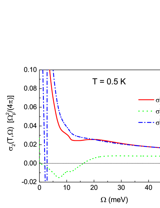
Figure 1: (Color online) The imaginary part $\sigma_{2}(T,\Omega)$ of the optical conductivity in units of $\Omega_{p}^{2}/(4\pi)$ as a function of the photon energy $\Omega$. The temperature is $T=0.5\,$K and the Pb electron-phonon spectral density was used with a superconducting critical temperature $T_{c}=7.2\,$K. The solid (red) curve is for the superconducting state (sc). The dotted (green) curve presents the case when $\sigma_{2}(T,\omega)$ is modified according to the prescription of Dordevic et al.Dordevic et al. (2014) (sc-m). Finally, the dashed-dotted (blue) curve presents the result for the Bogoliubov quasiparticles (bqp).

$\sigma(T,\Omega)$ in three cases. The solid (red) curve is the superconducting case based on the electron-phonon interaction spectral function $\alpha^{2}F(\omega)$ of PbMcMillan and Rowell (1965) and our Eqs. (2) and (3) for the optical conductivity with the impurity scattering rate $1/\tau_{\rm imp}=0$. Thus, we are considering the clean limit and only inelastic scattering is involved. The dashed-dotted (blue) curve is obtained from Eqs. (2) and (3) but including only BQP contributions, i.e. $P(\Omega)$ is formally set equal to zero in Eq. (3) while all other quantities remain unchanged. First, note that the main differences between these two results are confined to the photon energies up to $\sim 20\,$meV or about seven times the optical gap $2\Delta_{0}\simeq 2.8\,$meV. Beyond this the two curves have merged. For the superconducting case, $\sigma_{2}^{sc}(T,\Omega)$ goes to infinity as $\Omega$ tends to zero such that the $\lim_{\Omega\to 0}\Omega\sigma_{2}^{sc}(T,\Omega)=\rho_{s}\Omega_{p}^{2}/(4\pi)$. This limit provides a measure of the superfluid density $\rho_{s}$. For the BQP gas and the model of Dordevic et al.Dordevic et al. (2014) there is, of course, no superfluid density. It is very important for what will come later to note that for the BQP gas $\sigma_{2}^{bqp}(T,\Omega)$ has a zero-crossing below the optical gap. This does not occur in the superconducting state. This zero will have serious manifestations when we raise the temperature as we will in Sec. IV. The dotted (green) curve gives $\sigma_{2}^{sc-m}(T,\Omega)$ obtained from Eq. (11) according to the suggestion of Dordevic et al.Dordevic et al. (2014) We see that it differs from the other two curves at all photon energies and, in particular, does not merge with the solid (red) and dashed-dotted (blue) curves even at the highest energy considered here ($\sim 50\,$meV), where it is smaller by more than a factor of two. This has important implications for the behavior of the optical scattering rate. To understand why this is so we need to also consider the real part of the optical conductivity for these three cases. This is shown in Fig. 2.

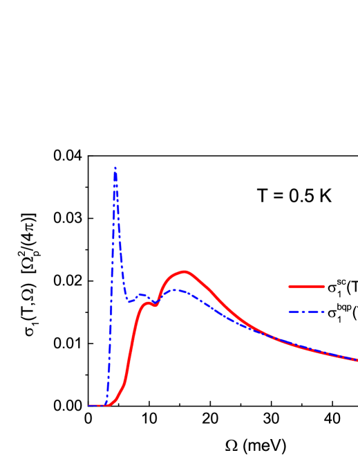
Figure 2: (Color online) The real part $\sigma_{1}(T,\Omega)$ of the optical conductivity in units of $\Omega_{p}^{2}/(4\pi)$ as a function of the photon energy $\Omega$. The temperature is $T=0.5\,$K and the Pb electron-phonon spectral density was used. The solid (red) curve presents the result for the superconducting state (sc) and the dashed-dotted (blue) curve is for the Bogoliubov quasiparticle gas (bqp).

Only two curves are considered because $\sigma_{1}(T,\Omega)$ is the same for the sc and sc-m cases. The solid (red) curve applies to the superconducting state while the dashed-dotted (blue) curve is for the BQP gas. Optical absorption starts at the finite photon energy $\Omega=2\Delta_{0}\simeq 2.8\,$meV because in both cases the quasiparticle excitation spectrum is gaped. Just above the optical gap the two responses show distinct behavior. The dashed-dotted (blue) curve for BQP has an inverse square root singularity associated with the onset of optical absorption while the solid (red) curve for the superconducting state, by contrast, rises slowly out of zero. In Appendix A we calculate the real part of the optical conductivity of a BQP gas in the clean limit of BCS theory. In this limit the spectral functions in Eq. (1) are Dirac delta-functions and the integrals can be done analytically. For the BQP case only the $A({\bf k},\omega)A({\bf k},\omega+\Omega)$ term appears. It results in two distinct contributions. An intraband and an interband piece. The intraband part does not contribute at $T=0$ as there is zero optical spectral weight in this Drude-like term in the clean limit. The interband contribution has the form (19) (see Appendix A)

$$\textrm{Re}\{\sigma^{bqp}_{\rm inter}(T=0,\Omega)\}\propto\frac{\Lambda}{\Omega^{2}}\frac{\Delta^{2}}{\sqrt{\Omega^{2}-(2\Delta^{2})}},\quad\textrm{for}\quad\Omega>2\Delta,$$ (12)

which we repeat here for the convenience of the reader. This inverse square root singularity is clearly seen in the dashed-dotted (blue) curve of Fig. 2. As we included inelastic scattering in our calculations, Eq. (12) is superimposed on a phonon assisted background. This background extends to large energies while the clean limit type contribution (12) is confined mainly to the region $\Omega=2\Delta$ to $4\Delta$. In contrast, the solid (red) curve for the superconducting state shows no interband divergence. This is traced to the fact that when the $A({\bf k},\omega)A({\bf k},\omega+\Omega)$ and $B({\bf k},\omega)B({\bf k},\omega+\Omega)$ in Eq. (1) are both included, the interband pieces cancel. (Class II matrix elements.) Consequently, only the phonon assisted processes are seen in the solid (red) curve. There is a phonon kink (a dip) in both (bqp) and (sc) curves at an energy which corresponds to the end of the phonon spectrum plus the optical gap. which falls around $\sim 13\,$meV. In the region beyond this energy the two curves of Fig. 2 show some deviations (never large) from each other but at $\sim 25\,$meV, or $\sim 8$ times the optical gap, they merge. It is important to understand that the interband transitions involved in Eq. (12) have nothing to do with relaxation processes but rather have mainly to do with the electronic band structure of the BQP gas, and exist even when no scattering is accounted for. Of course, the high energy part of the curves reflects the inelastic scattering and this region does carry information on relaxation processes which is our primary interest in this work. In the paper by Dordevic et al.Dordevic et al. (2014) the real part of the quasiparticle conductivity defined in Eq. (10) is that given by the solid (red) curve of Fig. 2. Thus, in all three cases of interest $\sigma_{1}(T,\Omega)$ is the same at high energies. ($\Omega\geq 25\,$meV). However, as we have seen in Fig. 1 only the superconducting state and BQP case merge when we consider the imaginary part of the optical conductivity $\sigma_{2}(T,\Omega)$ while the modified case of Dordevic et al.Dordevic et al. (2014) strongly deviates. This implies similar differences for the optical scattering rate defined in Eq. (8) as is seen in Fig. 3.

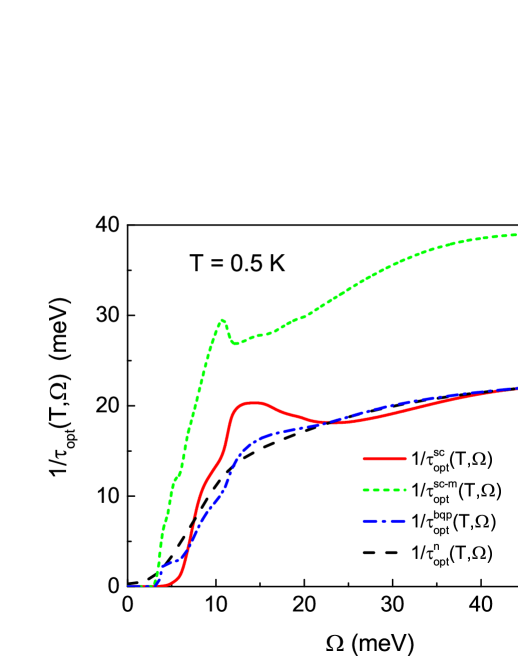
Figure 3: (Color online) The optical scattering rate $1/\tau_{\rm opt}(T,\Omega)$ which is related to the optical self-energy as a function of the photon energy $\Omega$. The temperature is $T=0.5\,$K and the Pb electron-phonon spectral density was used. The solid (red) curve is the superconducting state result (sc). The dotted (green) is for the superconducting state modified according to the prescription of Dordevic et al.Dordevic et al. (2014) (sc-m). The dashed-dotted (blue) curve presents the result for the Bogoliubov quasiparticle gas (bqp) and the dashed (black) curve applies to the normal state (n).

Staying for now with the high energy region we note, as expected, that the solid (red) and the dashed-dotted (blue) curves match perfectly while the dotted (green) curve for the modified superconducting case is larger than the other two by a factor of two. This can be understood entirely from the fact that $\sigma_{2}^{sc-m}(T,\Omega)$ is much smaller in this energy range than is $\sigma_{2}^{sc}(T,\Omega)$ or $\sigma_{2}^{bqp}(T,\Omega)$. We included in Fig. 3, for reference, normal state results as the dashed (black) curve. It agrees well with the superconducting state and the BQP gas but not with the dotted (green) curve which we will, therefore, not discuss further here because it does not conform to our expectation that at large $\Omega$ the presence of a gap in the quasiparticle excitation spectrum should no longer matter.

The deviations between the remaining three curves are in fact rather small at all energies except for two features. First, the solid (red) curve for the superconducting state shows a peak in the phonon assisted region between $\sim 10\,$meV to $\sim 20\,$meV which is not part of the other two curves. The deviations are of the order of $20\,\%$. Second, at energies below $\sim 6\,$meV the solid (red) curve rapidly goes to zero while the dashed-dotted (blue) curve shows a plateau before it eventually drops to zero. This plateau has its origin in the interband transitions. These are shown in Fig. 2 as a large prominent peak between, roughly, the energies $2\Delta(T)$ and $4\Delta(T)$. Returning to Fig. 3, below the optical gap the normal state dashed (black) curve is, of course, non-zero as there is no gap in this case.

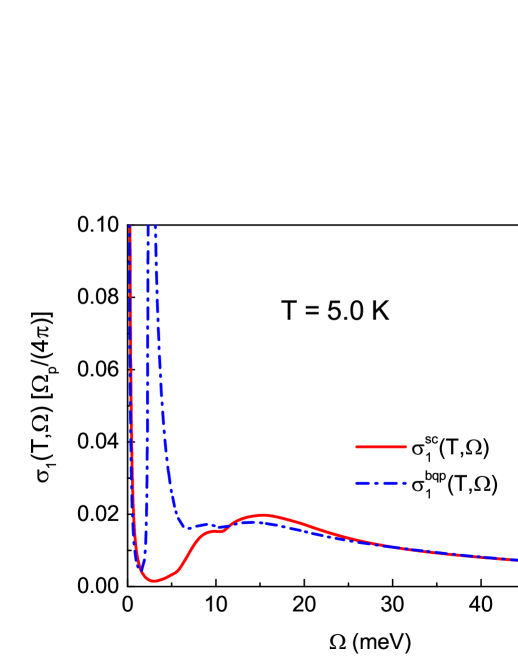
Figure 4: (Color online) Same as Fig. 2 but now the temperature was raised to $T=5\,$K. The Pb electron-phonon spectral density was used. The solid (red) curve applies to the superconducting state (sc) and the dashed-dotted (blue) curve to the Bogoliubov quasiparticle gas (bqp).

IV Finite temperature and impurity scattering

In this section the temperature was chosen to be large enough to expect results different from the $T=0.5\,$K case which is basically the zero temperature limit. In particular, we chose $T=5\,$K or $T/T_{c}\simeq 0.69$. This remains within the superconducting state but is sufficiently high that the optical gap is reduced from its $T=0$ value of $2.8\,$meV to $2.4\,$meV. Results for the real part of the optical conductivity are presented in Fig. 4. The dashed-dotted (blue) curve is for the BQP gas and the solid (red) curve is for the superconducting state. The change in the superconducting gap is most clearly seen in the dashed-dotted (blue) curve when compared with the equivalent curve of Fig. 2. There is now finite absorption at all $\Omega$ below the gap due to the existence of a small number of thermally excited quasiparticles at this elevated temperature, in contrast to the $T=0$ case for which the real part (absorptive part) of the optical conductivity is zero below the optical gap. The phonon region above the optical gap is, in contrast, not changed much from $T=0.5\,$K.

Results for the optical scattering rate are presented in Fig. 5.

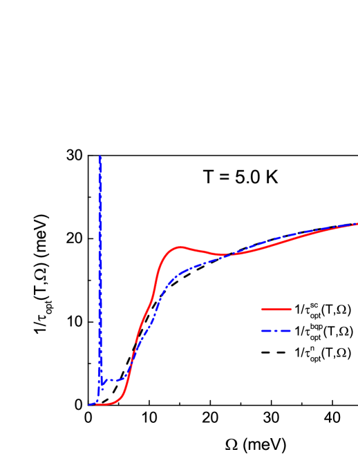
Figure 5: (Color online) The same as Fig. 3 for the optical scattering rate $1/\tau_{\rm opt}(T,\Omega)$ but now for $T=5\,$K. The solid (red) curve applies to the superconducting state (sc), the dashed-dotted (blue) curve to the Bogoliubov quasiparticle gas (bqp), and the dashed (black) curve to the normal state (n).

The three curves are $1/\tau^{sc}_{\rm opt}(T,\Omega)$, superconducting state [solid (red) curve], $1/\tau^{bqp}_{\rm opt}(T,\Omega)$, BQP gas [dashed-dotted (blue) curve], and $1/\tau^{n}_{\rm opt}(T,\Omega)$, normal state [dashed (black) curve]. These results are not very different from those of Fig. 3, normal state and BQP gas remain close above $6\,$meV. The superconducting state retains its peak in the range of 10 to $20\,$meV and the plateau just above the optical gap in the dashed-dotted (blue) curve remains as well. There is, however, a striking difference. A sharp peak has developed below the optical gap at $\Omega_{0}\simeq 2\,$meV. This is exactly the energy at which $\sigma_{2}^{bqp}(T,\Omega_{0})$ crosses zero. But, as seen in Fig. 4, $\sigma_{1}^{bqp}(T,\Omega_{0})$ is non-zero at this crossing and this is the origin of the peak seen in $\tau_{\rm opt}^{bqp}(T,\Omega_{0})$. As we have shown, $\sigma_{2}^{bqp}(T,\Omega)$ also has a zero-crossing (Fig. 1) at $T=0.5\,$K. This zero-crossing has no measurable consequences in the optical scattering rate however, because $\sigma_{1}^{bqp}(T\approx 0,\Omega)$ is zero below the optical gap in this case.

So far we did not include in our work static elastic residual impurity scattering, rather only inelastic scattering was considered. Eqs. (2) and (3) for the optical conductivity were written with a $i/\tau_{\rm imp}$ term and we now set $1/\tau_{\rm imp}=6.28\,$meV in Eqs. (22) for illustrative purposes. This affects both the real and imaginary part of the optical conductivity. In Fig. 6 we present results for the real part of the

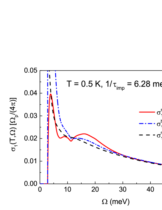
Figure 6: (Color online) The same as Fig. 2 for the real part of the optical conductivity, But now elastic impurity scattering with $1/\tau_{\rm imp}=6.28\,$meV is included. The scale on the vertical axis has been adjusted to make clear the Drude-like contribution seen (as a peak) just above the optical gap. This peak is not there when $1/\tau_{\rm imp}=0$, i.e. in the clean limit of inelastic scattering only. The solid (red) curve applies to the superconducting state (sc), the dashed-dotted (blue) curve to the Bogoliubov quasiparticle gas (bqp), and the dashed (black) curve to the normal state (n).

optical conductivity in the superconducting state. The solid (red) curve has now acquired a sharp peak just above the optical gap which was not there in Fig. 2 for the pure case ($1/\tau_{\rm imp}=0$). This peak is what remains when the Drude peak of the normal state shown as the the dashed (black) curve is cut off by the optical gap. In BCS theory this would be the only contribution to the optical conductivity. Here, the inelastic scattering provides additional absorption at higher energies. When $1/\tau_{\rm imp}=0$ this is the only contribution that remains. The Drude peak about $\Omega=0$ comes from the coherent part of the quasiparticle Green’s function $G$. At zero temperature and with no elastic scattering this contribution collapsed into a Dirac delta-function at the origin and, consequently, is not seen in Fig. 2. It contains approximately $1/(1+\lambda)$ of the optical spectral weight, where $\lambda$ is the electron-phonon mass enhancement parameter. This contribution broadens out into a Drude peak when $1/\tau_{\rm imp}$ is non-zero. To a good approximation this part of the normal state optical response can be written at $T=0$ asMarsiglio and Carbotte (2008)

$$\sigma_{1}^{\rm Drude}(T,\Omega)=\frac{\Omega_{p}^{2}}{4\pi}\frac{\Gamma/(1+\lambda)}{\Omega^{2}+[\Gamma/(1+\lambda)]^{2}}\frac{1}{1+\lambda},$$ (13)

with $\Gamma\equiv 1/\tau_{\rm imp}$. In the superconducting state this gets gaped with loss optical spectral weight transferred to the condensate. The phonon assisted processes (incoherent part) provide an additional contribution which contains the remaining optical spectral weight approximately proportional to $\lambda/(1+\lambda)$ and these are the only processes that show up at finite photon energies in Fig. 2 (pure case). Comparing the real part of the optical conductivity for the BQP gas $\sigma_{1}^{bqp}(T\approx 0,\Omega)$ [dashed-dotted (blue) curve] with impurities to its value in the clean limit shown in Fig. 2, we note that the interband peak just above the optical gap has been broadened. Also the secondary peak just below $10\,$meV in Fig. 2 has been modified to a shoulder.

The truncated Drude peak in the solid (red) curve of Fig. 6 also shows up as a peak in the optical scattering rate of Fig. 7 immediately above the optical gap. The normal state $1/\tau_{\rm opt}^{n}(T,\Omega)$ [dashed (black) curve],

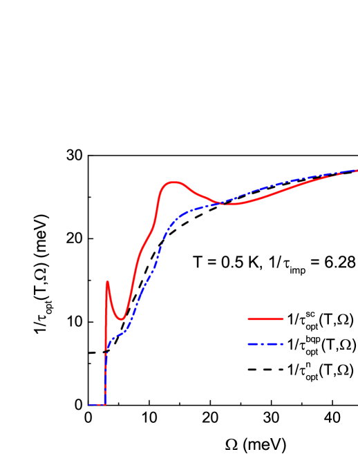
Figure 7: (Color online) The same as Fig. 3 for the optical scattering rate $1/\tau_{\rm opt}(T,\omega)$ including elastic impurity scattering $1/\tau_{\rm imp}=6.28\,$meV. The solid (red) curve applies to the superconducting state (sc), the dashed-dotted (blue) curve to the Bogoliubov quasiparticle gas (bqp), and the dashed (black) curve to the normal state (n).

however, has no optical gap and, consequently, no peak. However, it is finite at $\Omega=0$ and equal to the residual scattering rate. In general, it is the sum of $1/\tau_{\rm imp}$ plus the inelastic contribution of the previous section (pure case). At low photon energies the curve is flat and equal to $1/\tau_{\rm imp}$ because the inelastic contributions start from zero at $\Omega=0$ and remain small. In the other two curves we see that the absorption edge at $\Omega=2\Delta(T)$ has effectively sharpened, as compared with the pure case of Fig. 3, showing an initial vertical rise out of zero. At high energies the solid (red) curve, the dashed-dotted (blue) curve, and the dashed (black) curve merge. BQP and normal state curves are in fact close to each other at all photon energies above the optical gap. As before the superconducting case shows a peak in the phonon assisted region which is not part of the other two cases.

In Fig. 8 we present additional results based on the electron-phonon interaction spectral density if V₃Si.Carbotte (1990) (See inset.)

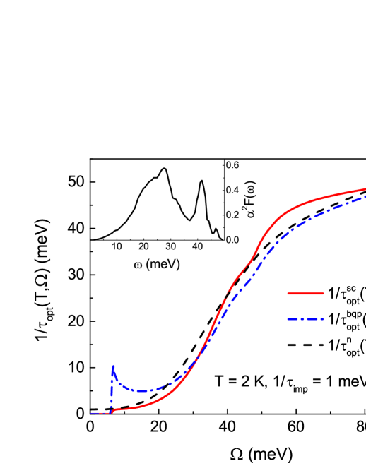
Figure 8: (Color online) The same as Fig. 7 (which was for Pb) but now the V₃Si electron-phonon interaction spectral density was used with an impurity scattering of $1/\tau_{\rm imp}=1\,$meV. The critical temperature $T_{c}=17.1\,$K, the temperature $T=2\,$K, and the gap $\Delta_{0}=2.9\,$meV. The solid (red) curve applies to the superconducting state (sc), the dashed-dotted (blue) curve to the Bogoliubov quasiparticle gas (bqp), and the dashed (black) curve to the normal state (n). The inset gives $\alpha^{2}F(\omega)$ for V₃Si.Carbotte (1990) The essential difference with Pb is that here the spectrum extends to $49\,$meV rather than $\sim 11\,$meV.

In contrast to Pb, this material is close to the weak coupling limit and also has a large maximum phonon energy of $\omega_{\rm max}=49\,$meV. The superconducting gap at $2\,$K is $\Delta_{0}=2.9\,$meV. The impurity scattering was taken to be $1/\tau_{\rm imp}=1\,$meV which remains in the clean limit, i.e. $\Delta_{0}\tau_{\rm imp}>1$ to be compared with the results presented in Fig. 7 for Pb where the dirty limit applies, i.e. $\Delta_{0}\tau_{\rm imp}\ll 1$ with $\Delta_{0}=1.4\,$meV and $1/\tau_{\rm imp}=6.3\,$meV. In the clean limit of Fig. 8 the rise in $1/\tau^{sc}(T,\Omega)$ [solid (red) curve] at the optical gap is small as compared to that in Fig. 7 because most of the Drude peak is now below the gap. For the BQP case [dashed-dotted (blue) curve] there is a sharp rise and a peak followed by a plateau which extends to approximately $20\,$meV before it starts to rise and crosses below $1/\tau^{sc}(T,\Omega)$ around $35\,$meV after which the two curves are never far apart. Except for a scale difference related to $\omega_{\rm max}$ these results are very similar to those of Pb. The physics is the same for weak or strong coupling and small or large maximum phonon energies $\omega_{\rm max}$.

In Fig. 9 we present a last set of results that illustrate

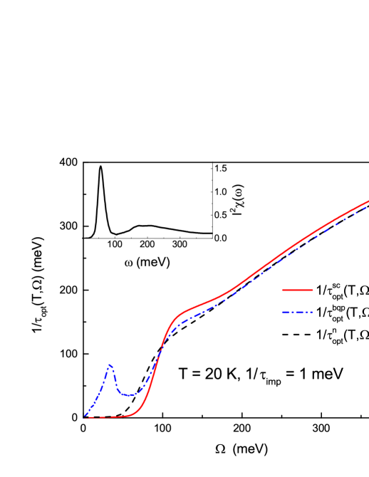
Figure 9: (Color online) The same as Fig. 8 but now the electron-boson interaction spectral density $I^{2}\chi(\omega)$ (see inset) obtained by Yang et al.Yang et al. (2009) for Hg1201 is used and the gap is taken to have $d_{x^{2}-y^{2}}$ symmetry which is apptopriate for the cuprates. The $T_{c}=90\,$K, the temperature $T=20\,$K, the elastic impurity scattering is $1/tau_{\rm imp}=1\,$meV, and the gap is $\Delta_{0}=19.5\,$meV. The solid (red) curve applies to the superconducting state (sc), the dashed-dotted (blue) curve to the Bogoliubov quasiparticle gas (bqp), and the dashed (black) curve to the normal state (n).

the effect of $d$-wave gap symmetry on the BQP optical scatterin rate. The calculations are based on the electron-boson interaction spectral density $I^{2}\chi(\omega)$ (see inset) obtained in the work by Yang et al. for Hg1201.Yang et al. (2009) To arrive at these results the Eliashberg equations of Appendix B had to be generalized to include gap anisotropy. These are found in Ref. Schachinger and Carbotte, 2003 along with the appropriate generalizations of Eqs. (2) and (3). Comparison of these results with those of Fig. 8 reveals the same qualitative behaviour except that the gap is distributed between $\Omega=0$ to $\Omega=2\Delta(T)=19.5\,$meV in accordance to $d_{x^{2}-y^{2}}$ gap symmetry. The plateau above the gap remains and beyond $\Omega\simeq 90\,$meV $1/\tau^{bqp}_{\rm opt}(T,\Omega)$ becomes close to $1/\tau^{sc}_{\rm opt}(T,\Omega)$ and $1/\tau^{n}_{\rm opt}(T,\Omega)$. The results presented are based on the optical conductivity within the CuO plane ($ab$-plane).

V Conclusions

We calculated the optical conductivity $\sigma^{sc}(T,\Omega)$ (superconducting state) and $\sigma^{bqp}(T,\Omega)$ (BQP gas) and compared the two. Of particular interest in such a comparison was the derived optical scattering rate which corresponds to the imaginary part of the optical self-energy. This optical constant was often highlighted in the experimental literature because it provided information on quasiparticle relaxation. What was directly accessible in experiment was the superconducting state optical scattering rate $1/\tau^{sc}_{\rm opt}(T,\Omega)$ while it was the BQP gas scattering rate $1/\tau^{bqp}_{\rm opt}(T,\Omega)$ which was more directly interpretable. Thus, the question arose as to how similar or different these two rates were. This was recognized in a recent paper by Dordevic et al.Dordevic et al. (2014) who attempted to factor out of the superconducting state optical data, the direct effect of the superfluid condensate and so access intrinsic quasiparticle properties. To accomplish this they advocated subtracting first from the imaginary part of the superconducting state optical conductivity, $\sigma^{sc}_{2}(T,\Omega)$ the Kramers-Kronig transform of the superfluid density $\rho_{s}$ which appears in the real part of $\sigma^{sc}(T,\Omega)$ as a Dirac delta-function at $\Omega=0$ of weight $\rho_{s}$. After this modification the optical scattering rate which we denoted $1/\tau^{sc-m}_{\rm opt}(T,\Omega)$ was computed. First, at photon energies twice the maximum phonon energy plus the optical gap energy (of the order of $26\,$meV for Pb) we found that superconducting and BQP gas scattering rates agree to within a few percent as we might have expected. In contrast, the sc-m case predicted that the scattering rate was larger by almost a factor of two in this energy region. Second, when we compared with the optical scattering rate $1/\tau^{n}_{\rm opt}(T,\Omega)$ obtained for the normal state, we find good agreement with the superconducting state and with $1/\tau^{bqp}_{\rm opt}(T,\Omega)$. This demonstrated that in this energy range the superconducting optical scattering rate, as has been widely defined in the literature, indeed provided a reliable measure of relaxation in both normal and BQP gas. This was not surprising since at these energies the superconducting gap is small as compared with the total energy involved.

In the phonon assisted energy region between 10 and $20\,$meV (in the specific case of Pb) a broad peak appeared in the optical scattering rate of the superconducting state which was not seen in either the normal state or the BQP gas. This translated into deviations of $\sim 20\,\%$, still rather modest. We also found that, at finite temperature, a sharp peak developed in the optical scattering rate of the BQP gas below the optical gap. Such a peak was neither present in the superconducting nor in the normal state. It was traced to a zero crossing of the imaginary part of the BQP gas’ optical conductivity. It is a signature of this crossing and is not directly related to a relaxation rate. Furthermore, from the optical gap energy to approximately twice this energy the BQP optical scattering rate had a plateau which was traced back to the interband transitions present in this case, even in the clean limit. However, above $\sim 6\,$meV $[\sim 4\Delta(T)]$ we found that when $1/\tau^{bqp}_{\rm opt}(T,\Omega)$ was compared with $1/\tau^{n}_{\rm opt}(T,\Omega)$ the agreement was almost as good as it was at high energies. Thus, normal state and BQP gas optical scattering rates were close to each other in the entire range of photon energies above twice the optical gap. This central conclusion remains true when finite residual scattering due to disorder is introduced, when the temperature is increased, when we go from strong coupling Pb with a soft phonon spectrum to weak coupling V₃Si with a large maximum phonon energy of $\sim 50\,$meV, and when gap anisotropy is considered. The specific example provided is for Hg1201, a cuprate with $d$-wave gap symmetry.

Appendix A

At zero temperature the real part of the dynamic optical conductivity associated with the BQP gas is given by Eq. (1) with only the $A({\bf k},\omega)A({\bf k},\omega+\Omega)$ term contained in the last square bracket. We get

$$\textrm{Re}\{\sigma^{bqp}(T=0,\Omega)\}=\frac{e^{2}}{2\Omega}v^{2}_{F}N(0)\int_{-\infty}^{\infty}\!d\epsilon\int_{-\Omega}^{0}\!d\omega\,A({\bf k},\omega)A({\bf k},\omega+\Omega).$$ (14)

Here, $N(0)$ is the normal state electronic density of states associated with energies $\epsilon\equiv\epsilon_{\bf k}$ taken at the chemical potential $\mu$ which we set to zero. In the BCS clean limit, i.e. no residual scattering and zero inelastic contribution, the spectral density $A({\bf k},\omega)$ reduces to two Dirac delta-functions of the form:

$$A(\epsilon_{\bf k},\omega)=u^{2}_{\bf k}\delta(\omega-\epsilon_{\bf k})+v^{2}_{\bf k}\delta(\omega+\epsilon_{\bf k}),$$ (15)

with

$$u^{2}_{\bf k} = \frac{1}{2}\left(1+\frac{\epsilon_{\bf k}}{E_{\bf k}}\right)$$

$$v^{2}_{\bf k} = \frac{1}{2}\left(1-\frac{\epsilon_{\bf k}}{E_{\bf k}}\right),$$ (16)

where

$$E_{\bf k}=\sqrt{\epsilon^{2}_{\bf k}+\Delta^{2}}.$$ (17)

Here $\Delta$ is the BCS gap and $2\Delta$ is the corresponding optical gap.

Substituting Eq. (15) for $A({\bf k},\omega)$ in Eq. (14) leads to an intraband and an interband contribution. The first is proportional to $\delta(\Omega)$ while the second contribution has a $\delta(2\omega+\Omega)$ factor. Specifically, we get, setting $\Lambda\equiv e^{2}v_{F}^{2}N(0)/2$:

$$\textrm{Re}\{\sigma^{bqp}_{\rm intra}(T=0,\Omega)\} \propto \frac{\Lambda}{\Omega}\delta(\Omega)\int_{-\infty}^{\infty}\!d\epsilon\int_{-\Omega}^{0}\!d\omega\,\left[u^{4}_{\bf k}\delta(\omega-E_{\bf k})+v^{4}_{\bf k}\delta(\omega+E_{\bf k})\right],$$

$$\textrm{Re}\{\sigma^{bqp}_{\rm inter}(T=0,\Omega)\} \propto \frac{\Lambda}{\Omega}\int_{-\infty}^{\infty}\!d\epsilon\int_{-\Omega}^{0}\!d\omega\,\delta(2\omega+\Omega)u^{2}_{\bf k}v^{2}_{\bf k}\left[\delta(\omega-E_{\bf k})+\delta(\omega+E_{\bf k})\right].$$ (18)

The first term, $\textrm{Re}\{\sigma^{bqp}_{\rm intra}\}$ involves intraband optical transitions and the second, $\textrm{Re}\{\sigma^{bqp}_{\rm inter}\}$, interband transitions. In each term, the Dirac delta-function $\delta(\omega-E_{\bf k})$ never clicks in the range of integration for $\omega$ and we are left with a single contribution involving only $\delta(\omega+E_{\bf k})$. The interband contribution works out to be

$$\textrm{Re}\{\sigma^{bqp}_{\rm inter}(T=0,\Omega)\}\propto\frac{\Lambda}{\Omega^{2}}\frac{\Delta}{\sqrt{\Omega^{2}-(2\Delta)^{2}}},$$ (19)

for $\Omega>2\Delta$ and zero for $\Omega<2\Delta$. The intraband contribution is zero as we expect at $T=0$. The interband transitions are seen in the dashed-dotted (blue) curve of Fig. 2. On the other hand, to get the real part of the dynamic optical conductivity in the superconducting state we need to include the $B({\bf k},\omega)B({\bf k},\omega+\Omega)$ term of Eq. (1) and this leads to a complete cancellation of the interband transitions, a well known effect for class II matrix elements. As seen in the solid (red) curve of Fig. 10 $\sigma^{sc}_{1}(T,\Omega)$ does not show an inverse square root singularity at $\Omega=2\Delta$ but rather starts from zero at that point. This behavior is different from that of the dashed-dotted (blue) curve for the BQP gas and, of course, from the normal state response [dashed (black) curve].

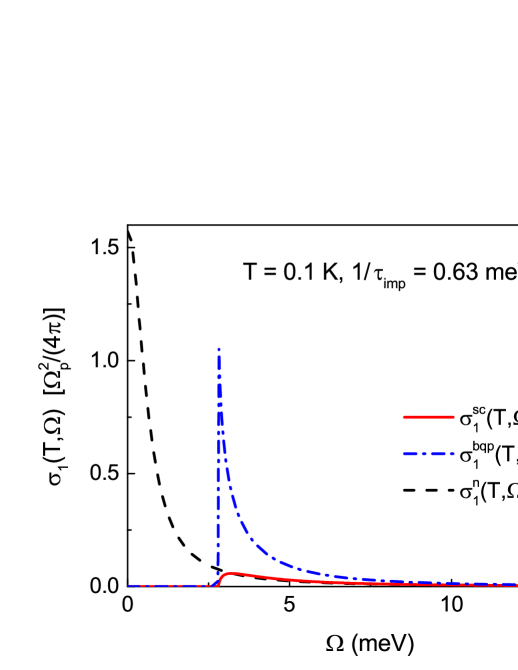
Figure 10: (Color online) The BCS real part of the optical conductivity $\sigma_{1}(T,\Omega)$ at $T=0.1\,$K and with elastic impurity scattering $1/\tau_{\rm imp}=0.63\,$meV. The superconducting gap $\Delta(0)=1.4\,$meV. The solid (red) curve applies to the superconducting state (sc), the dashed-dotted (blue) curve to the Bogoliubov quasiparticle gas (bqp), and the dashed (black) curve to the normal state (n).

Appendix B

It is most convenient to solve the Eliashberg equations as two coupled non-linear equations in an imaginary axis representation:Carbotte (1990)

$$\tilde{\Delta}(T,i\omega_{n})=\pi T\sum_{m}\left[\lambda(i\omega_{n}-i\omega_{m})-\mu^{\star}\right]\frac{\tilde{\Delta}(T,i\omega_{m})}{\sqrt{\tilde{\omega}^{2}(T,i\omega_{m})+\tilde{\Delta}^{2}(T,i\omega_{m})}},$$ (20a)

and

$$\tilde{\omega}(T,i\omega_{n})=\omega_{n}+\pi T\sum_{m}\lambda(i\omega_{n}-i\omega_{m})\frac{\tilde{\omega}(T,i\omega_{m})}{\sqrt{\tilde{\omega}^{2}(T,i\omega_{m})+\tilde{\Delta}^{2}(T,i\omega_{m})}}.$$ (20b)

Here, $T$ is the temperature, $\mu^{\star}$ is the Coulomb pseudo-potential, $\omega_{n}=\pi T(2n+1),n=0,\pm 1,\pm 2,\ldots$ the Matsubara frequencies, and $\lambda(i\omega_{n}-i\omega_{m})$ is given by:

$$\lambda(i\omega_{n}-i\omega_{m})=2\int_{0}^{\infty}\!d\Omega\,\frac{\Omega\alpha^{2}F(\Omega)}{\Omega^{2}+(\omega_{n}-\omega_{m})^{2}}.$$ (21)

Eqs. (20) are valid for any amount of electron-impurity scattering as this contribution cancels in these equations. This set of equations can be used to calculate thermodynamic properties, the penetration depth, etc.

If one wants to determine response functions, like the optical conductivity, the renormalized frequencies $\tilde{\omega}(T,\omega)$ and the gap function $\tilde{\Delta}(T,\omega)$ are required. These are obtained from Eqs. (20) by analytic continuation using an algorithm developed by F. Marsiglio et al.Marsiglio et al. (1988) and are denoted by $\tilde{\omega}_{\rm clean}(T,\omega)$ and $\tilde{\Delta}_{\rm clean}(T,\omega)$. If electron-impurity scattering described by an impurity scattering rate $1/\tau_{\rm imp}$ is present, one has to perform, in addition, the following renormalization:Marsiglio and Carbotte (1997)

$$\tilde{\omega}(T,\omega)=\tilde{\omega}_{\rm clean}(T,\omega)+\frac{i}{2\tau_{\rm imp}}\frac{\tilde{\omega}(T,\omega)}{\sqrt{\tilde{\omega}^{2}(T,\omega)-\tilde{\Delta}^{2}(\omega)}},$$ (22a)

and

$$\tilde{\Delta}(T,\omega)=\tilde{\Delta}_{\rm clean}(T,\omega)+\frac{i}{2\tau_{\rm imp}}\frac{\tilde{\Delta}(T,\omega)}{\sqrt{\tilde{\omega}^{2}(T,\omega)-\tilde{\Delta}^{2}(T,\omega)}},$$ (22b)

which have to be solved self consistently. The functions $\tilde{\omega}(T,\omega)$ and $\tilde{\Delta}(T,\omega)$ [either in the clean limit or renormalized according to Eqs. (22)] are then used in Eqs. (4) to (6) to determine the optical conductivity from Eq. (2).