Perturbative approach to the capacitive interaction between a sensor quantum dot and a charge qubit

Abstract

We consider the capacitive interaction between a charge qubit and a sensor quantum dot(SQD) perturbatively to the second order of their coupling constant at zero temperature by utilizing the method of non-equilibrium Green’s functions together with infinite-U Lacroix approximation and employing Majorana fermion representation for qubit isospin operators. The effect of back-actions on dynamics of the system is taken into account by calculating the self-energies and the Green’s functions in a self-consistent manner. To demonstrate the applicability of the method, we investigate relevant physical quantities of the system at zero and finite bias voltages. In the regime of weak SQD-qubit coupling, we find a linear relation between the stationary-state expectation values of the third component of the qubit isospin vector, $\left\langle\tau_{3}\right\rangle$, and the differential conductance of the SQD. Furthermore, our numerical results predict that the effect of SQD-qubit coupling on differential conductance of the SQD should be maximized at zero bias voltage. Moreover, we obtain an analytical expression to describe the behavior of the differential conductance of the SQD with respect to the qubit parameters. Our results at zero bias voltage are consistent with the results of numerical renormalization group method.

I Introduction

Typically, the state of a solid state qubit could be indirectly extracted by measuring the conductance of a current carrying electro-meter which is capacitively coupled to the qubit. This detector, which could be realized in the experiment by a quantum point contact(QPC)aleiner1997 ; gurvitz1997 ; nature02693 ; korotkov2001continuous ; goan2001continuous ; stace2004continuous ; engel2004measurement ; luo2013 or a single electron transistor(SET)schoelkopf1998 ; nakamura1999coherent ; aassime2001radio ; lu2003 ; astafiev2004 ; lahaye2004approaching ; turek2005single ; barthel2010 , provides us with measurements of the charge fluctuations of qubit. The usage of SETs are however more advantageous to the QPCs because of their much more sensitivity to the charge fluctuationsbarthel2010 . In practice, the coupling of the sensor quantum dot(SQD) of the SET with qubit is made so weak in order to reduce the effect of measurements on the qubit state. But, no matter how much it is weak, the system inevitably suffers from coupling effects which results in a coherent back-action on the qubit dynamics and renormalization of the system energy levels.zorin1996 ; grishin2005

Using SET as a qubit detector has been the subject of several theoretical studiesmakhlin2001quantum ; PhysRevLett.84.5820 ; makhlin2000statistics ; korotkov2001selective ; gurvitz2005 ; gurvitz2008 ; shnirman1998 ; mozyrsky2004quantum ; oxtoby2006sensitivity ; emary2008quantum ; schulenborg2014detection ; hell2014 ; hell2016 . Much works have been devoted to investigate the time dependent dynamics of the reduced density matrix of the system with considering the leading order tunneling processes in the SET and ignoring the back-action of qubit and SET on each othermakhlin2000statistics ; korotkov2001selective ; gurvitz2005 ; gurvitz2008 . The problem of considering the effects of back-actions on the SET-qubit system in the presence of external bias were also studied in Refs.shnirman1998, ; mozyrsky2004quantum, ; oxtoby2006sensitivity, ; emary2008quantum, ; schulenborg2014detection, ; hell2014, ; hell2016, . Recently, Hell et al.hell2014 ; hell2016 studied the coherent back-action of the measurements on the SET-qubit system in the presence of finite bias by deriving Markovian kinetic equations for the system with considering next to the leading order corrections into the tunneling processes of the SET and the effects of energy levels’s renormalization of the system.

Here, we consider the application of the method of non-equilibrium Green’s functions for describing the non-equilibrium dynamics of the SET-qubit system. We calculate the steady-state non-equilibrium Green’s functions of the system at zero temperature using second order self-energies of the capacitive coupling between SQD and qubit. Due to the lack of applicability of the Wick’s theorem for Pauli operators, we utilize the Majorana Fermion representationtsvelik1992new ; mao2003spin ; shnirman2003spin for the qubit isospin operators by which a systematic diagrammatic perturbative expansion of the system’s Green’s functions become possible. In order to take into account strong electron-electron interaction on the SQD, which is necessary to keep it in the Coulomb blockade regime, we employ the infinite-U Lacroix approximationlacroix1981density to calculate the bare Green’s functions of SQD. The back-action effects on the average occupations of SQD and qubit are accounted for by calculating the self-energies and the Green’s functions self-consistently. Using the calculated interacting Green’s functions of the system, we investigate the density of states of the SQD and the steady-state expectation value of the third component of the isospin operator of the qubit, $\left\langle\tau_{3}\right\rangle$. Furthermore, we determine the differential conductance of SQD at zero and finite bias voltages and show that there is a linear relation between SQD’s differential conductance and the steady-state expectation value $\left\langle\tau_{3}\right\rangle$. We check the accuracy of our results at zero bias by comparing them with the results obtained from numerical renormalization group(NRG) methodbulla2008numerical .

Our approach differs basically from density matrix based approachesbreuer2002theory . In the latter, it is the coupling of SQD with electrodes which is considered perturbatively for calculating the reduced density matrix of the subsystem and the possible partial coherencies between different charge states of the SQD during tunneling processes are ignored trivially. Instead, in our approach, the parameter that is used for perturbatively obtaining the Green’s functions of the system is the capacitive coupling between SQD and qubit while the effects of coupling between SQD and metallic electrodes are incorporated non-perturbatively into the Green’s functions of SQD, which retains the possible partial coherencies of SQD’s charge states.

The paper is organized as follows: In Sec. II.1, the model Hamiltonian is presented. Then in Sec. II.2, we present the derivation of non-equilibrium Green’s functions of the SQD-qubit system. After that, in Sec.II.3, we give some expressions for relating different physical quantities of the system with the Green’s functions. We present our numerical results in Sec. III. Then, in Sec. IV, we give a summary of our work and some concluding remarks related to it.

II Theoretical formalism

II.1 Model Hamiltonian

Figure 1: (Color online) Schematic representation of the model system. The sensor quantum dot, characterized with gate voltage $\varepsilon_{d}$ and on-site interaction $U$, coupled to two metallic leads and simultaneously interacts capacitively with one double quantum dot through interaction constants $\lambda_{+}$ and $\lambda_{-}$. The on-site energies of DQD are $\pm\omega_{0}$ and the tunneling energy between its dots is specified by $\Delta/2$.

Our model system, as is depicted in Fig.1, consists of a SQD in a Coulomb blockade regime tunnel coupled to two metallic electrodes while simultaneously interacts capacitively with a charge qubit which is modeled by a double quantum dot(DQD). The total Hamiltonian of the system can be written as

$$\mathcal{H}=\mathcal{H}_{SET}+\mathcal{H}_{DQD}+\mathcal{H}_{I}.$$ (1)

The first term is the Hamiltonian of SET which is given by

$$\mathcal{H}_{SET} =\underset{\nu}{\sum}\varepsilon_{d}\,c_{d,\nu}^{\dagger}c_{d,\nu}+Un_{d,\uparrow}n_{d,\downarrow}+$$

$$\underset{k,\alpha,\nu}{\sum}(\varepsilon_{k}+\mu_{\alpha})\,c_{k,\alpha,\nu}^{\dagger}c_{k,\alpha,\nu}+t_{\alpha}\,\left(c_{k,\alpha,\nu}^{\dagger}c_{d,\nu}+H.c\right),$$ (2)

where the operator $c_{d,\nu}^{\dagger}\left(c_{d,\nu}\right)$ creates(annihilates) an electron with spin $\nu=\uparrow,\downarrow$ in the SQD, $n_{d,\nu}=c_{d,\nu}^{\dagger}c_{d,\nu}$ is the spin dependent electron occupation operator of SQD, $\varepsilon_{d}$ is the applied gate voltage and $U$ is the on-site electron-electron interaction energy in SQD. Similarly, the operator $c_{k,\alpha,\nu}^{\dagger}$$\left(c_{k,\alpha,\nu}\right)$ is the corresponding operator for electron creation(annihilation) with energy $\varepsilon_{k}$ in the left and right leads ($\alpha=L,R$), each of which are treated as half-filled quasi-one-dimensional normal metals with chemical potentials $\mu_{L}$ and $\mu_{R}$, respectively. The coupling of the SQD with each lead is assumed to be energy and spin independent and characterized by a hybridization constant, $t_{L,R}$.

The second term in Eq.(1) is the Hamiltonian of charge qubit, which is modeled as a double quantum dotgorman2005charge containing only one electron, with on-site energies $\pm\frac{\omega_{0}}{2}$ and hybridization energy $\frac{\Delta}{2}$. Representing the state of the electron on each of DQD’s dots by $\left|+\right\rangle$ and $\left|-\right\rangle$, in terms of isospin operators $\left(\tau_{1},\tau_{2},\tau_{3}\right)$ the DQD’s Hamiltonian takes the form

$$\mathcal{H}_{DQD} =-\frac{\omega_{0}}{2}\tau_{3}+\frac{\Delta}{2}\tau_{1}.$$ (3)

The last term in Eq.(1) is the capacitive interaction between SQD and DQD which is $2n_{d}(\lambda_{+}n_{+}+\lambda_{-}n_{-})$, where $\lambda_{+,-}$ is an interaction constant and $n_{d}=n_{d,\uparrow}+n_{d,\downarrow}$ is the total electron number operator of SQD. Furthermore, $n_{+,-}$ represents the occupation number operator of each dots of the DQD. By using the relation $n_{\pm}=\frac{1}{2}(1\pm\tau_{3})$ and an appropriate renormalization of $\varepsilon_{d}$, the interaction can be expressed as $\lambda n_{d}\tau_{3},$ where $\lambda\equiv\lambda_{+}-\lambda_{-}$. In addition, for later convenience, we explicitly take into account the mean-field back-action effects by adding and subtracting the operator $A=\lambda\left(\left\langle n_{d}\right\rangle\tau_{3}+\left\langle\tau_{3}\right\rangle n_{d}\right)$ to the total Hamiltonian. This modifies the on-site energies of the SQD and DQD to $\tilde{\varepsilon}_{d}=\varepsilon_{d}+\lambda\left\langle\tau_{3}\right\rangle$ and $\tilde{\omega}_{0}=\omega_{0}-2\lambda\left\langle n_{d}\right\rangle$, respectively, and then the interaction term of Hamiltonian becomes

$$\mathcal{H}_{I}=\lambda(n_{d}-\left\langle n_{d}\right\rangle)(\tau_{3}-\left\langle\tau_{3}\right\rangle).$$ (4)

In order to use perturbation theory we need to express the isospin operators in terms of Majorana fermion operators byshnirman2003spin

$$\tau_{a}=-i\epsilon_{abc}\eta_{b}\eta_{c},$$ (5)

for $a,b,c=1,2,3$, where $\epsilon_{abc}$ is the Levi-Civita antisymmetric tensor and $(\eta_{1},\eta_{2},\eta_{3})$ are three Majorana fermion operators satisfying usual fermionic equal-time anti-commutation relation $\{\eta_{a},\eta_{b}^{\dagger}\}=\delta_{a,b}$ with $\eta_{a}^{\dagger}=\eta_{a}$.

II.2 Non equilibrium Green’s functions

The non-equilibrium Green’s function method is a usual choice to study out of equilibrium systemsstefanucci2013nonequilibrium . We will treat $\mathcal{H}_{SQD}+\mathcal{H}_{DQD}$ and $\mathcal{H}_{I}$ as the non-interacting and interaction parts of Hamiltonians, respectively. A complete description of the non-equilibrium steady-state of a system requires the knowledge of four Green’s functions, which we choose the retarded, advanced, lesser and greater, defined, respectively, for the non-interacting system as

$$g_{s,mn}^{R}\left(t,t^{\prime}\right)=-i\theta(t-t^{\prime})\left\langle\left\{\Psi_{s,m}\left(t\right),\Psi_{s,n}^{\dagger}\left(t^{\prime}\right)\right\}\right\rangle_{0},$$ (6a)

$$g_{s,mn}^{A}\left(t,t^{\prime}\right)=i\theta(t^{\prime}-t)\left\langle\left\{\Psi_{s,m}\left(t\right),\Psi_{s,n}^{\dagger}\left(t^{\prime}\right)\right\}\right\rangle_{0},$$ (6b)

$$g_{s,mn}^{<}\left(t,t^{\prime}\right)=i\left\langle\Psi_{s,n}^{\dagger}\left(t^{\prime}\right)\Psi_{s,m}\left(t\right)\right\rangle_{0}$$ (6c)

and

$$g_{s,mn}^{>}\left(t,t^{\prime}\right)=-i\left\langle\Psi_{s,m}\left(t\right)\Psi_{s,n}^{\dagger}\left(t^{\prime}\right)\right\rangle_{0},$$ (6d)

where $s=d,\eta$ determines the corresponding subsystem for which the Green’s functions are defined and $m,n$ represent degrees of freedom for the corresponding subsystem, that is, in the case of SQD, $\Psi_{d,m}=c_{d,m}$ with $m=\uparrow,\downarrow$ while for DQD, $\Psi_{\eta,m}=\eta_{m}$ with $m=1,2,3$. In addition, $\left\langle\ldots\right\rangle_{0}$ is the expectation value with respect to the ground-state of $\mathcal{H}_{SQD}+\mathcal{H}_{DQD}$ at zero temperature. In the sequel, the term interacting/non-interacting is used to account for the interaction between SQD and DQD and not for the on-site interactions in the SQD. Also, we will present non-interacting and interacting Green’s functions by $g$ and $\mathcal{G}$, respectively. Furthermore, because our Hamiltonian does not explicitly depend on time, the Green’s functions become functions of time differences only and it is therefore more preferable to express them in the frequency space by Fourier transformation.

The inclusion of interactions is performed by using the Dyson equation through which the exact retarded Green’s function of the system could be determined by

$$\mathcal{G}^{R}\left(\omega\right) =\left[\mathcal{G}^{A}\left(\omega\right)\right]^{\dagger}$$

$$=g^{R}\left(\omega\right)+g^{R}\left(\omega\right)\Sigma^{R}\left(\omega\right)\mathcal{G}^{R}\left(\omega\right),$$ (7)

while the exact lesser Green’s function has the form

$$\mathcal{G}^{<}\left(\omega\right)=\mathcal{G}^{R}\left(\omega\right)\Sigma^{<}\left(\omega\right)\mathcal{G}^{A}\left(\omega\right),$$ (8)

where $\Sigma^{R,<}\left(\omega\right)$ stands for the total proper retarded and lesser self-energies of the system. The greater Green’s function is then obtained using $\mathcal{G}^{>}\left(\omega\right)=\mathcal{G}^{A}\left(\omega\right)-\mathcal{G}^{R}\left(\omega\right)+\mathcal{G}^{<}\left(\omega\right)$.

II.2.1 Green’s functions of SQD

In order to maximize the sensitivity of the SET, the energy level of SQD should be tuned to the flank of the Coulomb blockade peak. In this regime, the co-tunneling processes between SQD and leads become dominant and the conventional sequential tunneling approximations ceased to be applicable for describing the state of the SQD. Therefore we use the infinite-U Lacroix approximation, which is believed to consider co-tunnelings in the coulomb-blockade regime, in order to obtain the Green’s functions of SQD, $g_{d}^{R}$, which will be used later on as building blocks of the self-energies. By using Eq.($17$) of Ref.Roermund, , we obtain the Fourier transform of the diagonal elements of the SQD’s retarded Green’s function matrix as

$$g_{d,\nu\nu}^{R}\left(\omega\right)=\frac{1-\left\langle n_{d,\bar{\nu}}\right\rangle+P_{\nu}\left(\omega\right)}{\omega+i\delta-\tilde{\varepsilon}_{d}+i\left(\Gamma_{L}+\Gamma_{R}\right)-Q_{\nu}\left(\omega\right)},$$ (9)

where $\delta$ is an infinitesimal positive constant and $\Gamma_{L,R}\equiv\pi|t_{L,R}|^{2}\rho_{0}$ is the broadening of the SQD’s energy level due to its coupling to the leads in the standard wide-band limit in which the density of states of the leads, $\rho_{0}$, is assumed to be independent of energy. Furthermore,

$$P_{\nu}\left(\omega\right)=\underset{\alpha=L,R}{\sum}\frac{\Gamma_{\alpha}}{\pi}\int d\omega_{1}\frac{g_{d,\nu\nu}^{A}\left(\omega_{1}\right)f_{\alpha}\left(\omega_{1}\right)}{\omega+i\delta-\omega_{1}}$$ (10a)

and

$$Q_{\nu}\left(\omega\right)=\underset{\alpha=L,R}{\sum}\frac{\Gamma_{\alpha}}{\pi}\int d\omega_{1}\frac{\left(1+i\Gamma g_{d,\nu\nu}^{A}\left(\omega_{1}\right)\right)f_{\alpha}\left(\omega_{1}\right)}{\omega+i\delta-\omega_{1}},$$ (10b)

where $f_{L,R}\left(\omega\right)=\theta\left(\mu_{L,R}-\omega\right)$ and $\theta\left(...\right)$ is the standard Heaviside-theta function. For the non-interacting lesser Green’s function of SQD, $g_{d}^{<}\left(\omega\right)$, we have

$$g_{d}^{<}\left(\omega\right)=g_{d}^{R}\left(\omega\right)\Sigma_{d}^{(NG)<}\left(\omega\right)g_{d}^{A}\left(\omega\right),$$ (11)

where $\Sigma_{d}^{(NG)<}$ is the lesser self-energy calculated using the NG ansatzNGNG

$$\Sigma_{d}^{(NG)<}\left(\omega\right)=\left(\left[g_{d}^{R}\left(\omega\right)\right]^{-1}-\left[g_{d}^{A}\left(\omega\right)\right]^{-1}\right)\underset{\alpha=L,R}{\sum}\frac{\Gamma_{\alpha}f_{\alpha}\left(\omega\right)}{\Gamma}.$$ (12)

Using the self-energies of SQD, which are given in Appendix A, the interacting retarded and lesser Green’s functions of SQD can be obtained as

$$\mathcal{G}_{d}^{R}\left(\omega\right)=g_{d}^{R}\left(\omega\right)+g_{d}^{R}\left(\omega\right)\Sigma_{d}^{(2nd)R}\left(\omega\right)\mathcal{G}_{d}^{R}\left(\omega\right)$$ (13)

and

$$\mathcal{G}_{d}^{<}\left(\omega\right)=\mathcal{G}_{d}^{R}\left(\omega\right)\left(\Sigma_{d}^{(NG)<}\left(\omega\right)+\Sigma_{d}^{(2nd)<}\left(\omega\right)\right)\mathcal{G}_{d}^{A}\left(\omega\right).$$ (14)

II.2.2 Green’s functions of DQD

Using the method of equations of motion, the Fourier transform of the non-interacting retarded Green’s functions of DQD, $g_{\eta}^{R}$, can be computed from the following set of nine equations

$$\left(\omega+i\delta\right)g_{\eta,mn}^{R}= \delta_{mn}+\delta_{1m}\tilde{\omega}_{0}g_{\eta,2n}^{R}-$$

$$\delta_{2m}\left(\tilde{\omega}_{0}g_{\eta,1n}^{R}+\Delta g_{\eta,3n}^{R}\right)+\delta_{3m}\Delta g_{\eta,2n}^{R},$$ (15)

where $m,n=1,2,3$ and $\delta_{mn}$ is the Kronecker delta. The solution of the above equations in matrix form is

$$g_{\eta}^{R}\left(\omega\right)=\left(\begin{array}[]{ccc}\omega+i\delta&-i\tilde{\omega}_{0}&0\\ i\tilde{\omega}_{0}&\omega+i\delta&i\Delta\\ 0&-i\Delta&\omega+i\delta\end{array}\right)^{-1}.$$ (19)

Accordingly, the non-interacting lesser Green’s function of DQD is

$$g_{\eta}^{<}\left(\omega\right)=-2iIm\left[g_{\eta}^{R}\left(\omega\right)\right]f\left(\omega\right),$$ (20)

where $f\left(\omega\right)=\theta\left(-\omega\right)$.

Now we can use the self-energies of DQD, which are derived in Appendix A, to calculate the interacting retarded and lesser Green’s functions of DQD

$$\mathcal{G}_{\eta}^{R}\left(\omega\right)=g_{\eta}^{R}\left(\omega\right)+g_{\eta}^{R}\left(\omega\right)\Sigma_{\eta}^{(2nd)R}\left(\omega\right)\mathcal{G}_{\eta}^{R}\left(\omega\right)$$ (21)

and

$$\mathcal{G}_{\eta}^{<}\left(\omega\right)=\mathcal{G}_{\eta}^{R}\left(\omega\right)\Sigma_{\eta}^{(2nd)<}\left(\omega\right)\mathcal{G}_{\eta}^{A}\left(\omega\right).$$ (22)

II.3 Physical quantities

By using the definition of lesser Green’s function, Eq.(6c), the expectation values of $n_{d}$ and $\tau_{3}$ are

$$\left\langle n_{d}\right\rangle=-\frac{i}{2\pi}\int d\omega Tr\left[\mathcal{G}_{d}^{<}\left(\omega\right)\right]$$ (23)

and

$$\left\langle\tau_{3}\right\rangle=-2\int\frac{d\omega}{2\pi}\mathcal{G}_{\eta,12}^{<}\left(\omega\right).$$ (24)

Furthermore, the average electric current through SQD in the steady-state could be calculated by

$$I=-\frac{e}{\hbar}\int\frac{d\omega}{2\pi}\Gamma_{L}Tr[Im[\mathcal{G}_{d}^{<}\left(\omega\right)+2\mathcal{G}_{d}^{R}\left(\omega\right)f_{L}\left(\omega\right)],$$ (25)

from which we can obtain the differential conductance of the SQD through $G=\frac{dI}{dV_{b}}$.

For future reference, we also define the “signal differential conductance” of the SQDbarthel2010 ; petta , which is defined as the difference of the SQD’s conductance in the presence of DQD and in the absence of it. It is represented by

$$\delta G=G_{\lambda\neq 0}-G_{\lambda=0}.$$ (26)

III Results and discussions

Here we present our numerical results for zero and finite bias voltages. We calculate self-consistently the self-energies and the Green’s functions of the system (see Appendix B for a brief outline of our self-consistent calculations method). The calculations are performed at zero-temperature $T=0$ and $\Gamma=\Gamma_{L}+\Gamma_{R}$ is taken as unit of energy. Furthermore, we take $\hbar=e=c=1$. The finite bias is established by considering a symmetric bias voltage between two metallic lead as $\mu_{L}=-\mu_{R}=\frac{V_{b}}{2}$. In zero bias, we check our results by comparing them with NRG results which are obtained by utilizing “NRG ljubljana”zitko package. In all NRG calculations we set the logarithmic discretization parameter to $\Lambda=2$ and kept up to $1000$ states for each iteration diagonalizations.

III.1 Spectral densities and average occupation values

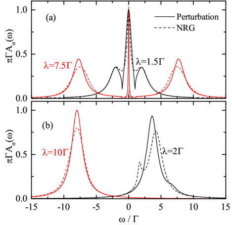
Figure 2: Comparison of single spin spectral densities of SQD calculated by perturbation method(full lines) with NRG method(dashed lines) with $U=0$, $\Delta=\Gamma$ and $V_{b}=0$. For the cases (a) $\varepsilon_{d}=0$, $2\lambda=\omega_{0}=3\Gamma,15\Gamma$ and (b) $\varepsilon_{d}=2\Gamma$, $\lambda=\frac{2}{3}\omega_{0}=2\Gamma,10\Gamma$.

In Fig.2, we compare the single spin QD’s local density of states, $A_{\sigma}(\omega)=-\frac{1}{\pi}Im[\mathcal{G}_{d,\sigma\sigma}^{R}(\omega)]$, obtained from our perturbative approach and NRG method. For simplicity, we take $U=0$ and fix the value of $\Delta$ to $\Gamma$, while we set different values to the $\lambda,\text{ }\omega_{0}\text{ and }\varepsilon_{d}$. In Fig.2(a), for the particle-hole symmetric case, $\varepsilon_{d}=0$ and $2\lambda=\omega_{0}$, we see good agreement between perturbative results and NRG except the rate of narrowing of the central peak and the height of the broad sidebands in the case of large $\lambda$s. In Fig.2(b), we show density of states for two particle-hole asymmetric configurations. The position of the broad peaks are in good agreement with NRG whereas their heights differ with it.

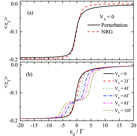
Figure 3: Average values of $\tau_{3}$ with respect to $\varepsilon_{d}$ for $\omega_{0}=0$, $\Delta=10^{-1}\Gamma$ and $\lambda=10^{-2}\Gamma$ at (a) zero bias and (b) finite bias.

Next we consider the presence of large on-site interactions on the SQD(infinite $U$) and focus on the weak-coupling parameter regime where the condition $\lambda\ll\Delta\ll\Gamma$ is satisfied. We set the energy difference between the two dots of DQD to zero, $\omega_{0}=0$, and study the average occupation values of qubit for different gate voltages of SQD in Fig.3. Generally, it is expected that the value of $\left\langle\tau_{3}\right\rangle$ becomes zero, i.e. $\left(\left\langle n_{\pm}\right\rangle=\frac{1}{2}\right)$, when there is no electron in SQD and by the presence of an electron on SQD, the $\left\langle\tau_{3}\right\rangle$ acquires a negative value to recover itself in the new potential energy of the qubit. In Fig.3(a) the average values $\left\langle\tau_{3}\right\rangle$, obtained separately by our self-consistent method and NRG, are depicted as a function of $\varepsilon_{d}$ for fixed $\Delta=10^{-1}$ and $\lambda=10^{-2}$ when there is no applied bias. We see almost good agreement with NRG. In the presence of finite bias voltages, as is shown in Fig.3(b), we see that by increasing bias voltages, a step starts to appear in the average values $\left\langle\tau_{3}\right\rangle$ in the range $-\frac{V_{b}}{2}<\varepsilon_{d}<\frac{V_{b}}{2}$, where the SQD has merely the same probability for being occupied or unoccupied and therefore $\left\langle\tau_{3}\right\rangle$ acquires a mid-value between zero and its minimum value.

III.2 Differential conductance

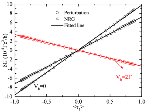
Figure 4: Plot of $\delta G$ calculated by pertubative method(circles) and NRG method(triangles) with respect to $\left\langle\tau_{3}\right\rangle$ in zero bias(black) and finite bias(red) voltages with $\varepsilon_{d}=0$, $\Delta=10^{-1}\Gamma$, $\lambda=10^{-2}\Gamma$.

For a SQD with $U=0$ and in the weak-coupling parameter regime, we can find an analytical expression for $\delta G$ which clearly shows linear relation with $\left\langle\tau_{3}\right\rangle$ (see appendix C for a derivation). Our numerical results for this case are also giving this linear relation perfectly (not shown here). On the other hand, in the case of a SQD with infinite $U$, due to the requirement of self-consistent calculations, obtaining an analytical expression for $\delta G$ is seems to be impossible, at least in the context of the NEGF formalism. Thus, in order to check the linear dependence of $\delta G$ on $\left\langle\tau_{3}\right\rangle$, we only concentrate on numerical results. In Fig.4, our numerical results for $\delta G$ as a function of $\left\langle\tau_{3}\right\rangle$ at zero and finite bias voltages are shown. We see that our perturbative results(circles) are fitted entirely to a line which clearly demonstrates the linear dependence of $\delta G$ on $\left\langle\tau_{3}\right\rangle$. An important feature in Fig.4 is the linear dependence of NRG results(triangles) for $\delta G$ with respect to $\left\langle\tau_{3}\right\rangle$ at zero bias. These NRG linear dependence could be thought of as a complementary confirmation for our observations although its line slope differs slightly from our perturbative results.

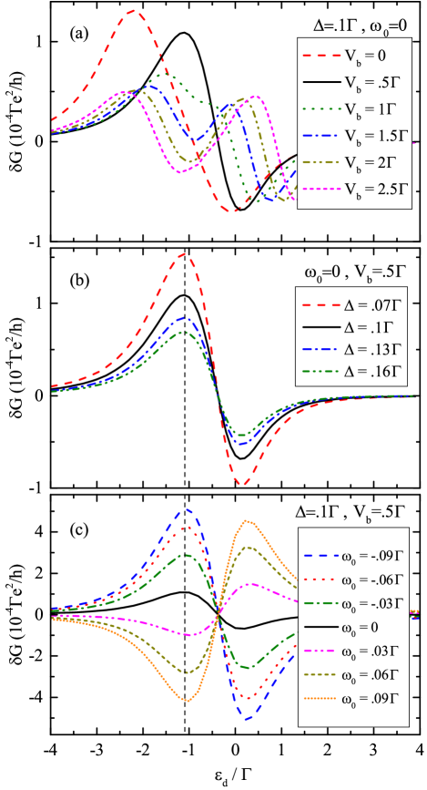
Figure 5: Differential signal conductance of SQD as a function of $\varepsilon_{d}$ for $\lambda=10^{-2}\Gamma$ with respect to (a)$V_{b}$, (b)$\Delta$ and (c)$\omega_{0}$.

In Fig.5, the dependence of $\delta G$ on the various parameters of the system is shown. In Fig.5(a), $\delta G$ is depicted as a function of $\varepsilon_{d}$ for different bias voltages while the values of $\Delta$, $\lambda$ and $\omega_{0}$ are kept fixed. We see that the curves of $\delta G$ go from an infinitesimal positive value for $\varepsilon_{d}\ll 0$ to an infinitesimal negative value for $\varepsilon_{d}\gg 0$ while for intermediate values of $\varepsilon_{d}$, they show some oscillations. By increasing the value of $V_{b}$, the oscillations change from a “one peak one dip” to a “two peak two dip” shape and also the positions of the peaks/dips are pushed from the center. Another remarkable feature is the decreasing of the amplitude of the $\delta G$ curves by increasing the bias voltage. In other words, we predict that the amplitudes for oscillations of signal differential conductances are maximized at zero bias voltage. Next, we study the impact of changing $\Delta$ on $\delta G$ in Fig.5(b). We see that increasing $\Delta$ has a reduction effect on $\delta G$ and decreases the amplitude of the differential signal conductances. The other parameter of the system which should have some effects on $\delta G$ is the energy difference between the two quantum dots of the charge qubit ($\omega_{0}$). In Fig.5(c), we investigate the impact of different values of $\omega_{0}$ on $\delta G$. We see that the position $\varepsilon_{d}$ of the peaks are almost intact, however, the amplitudes of the $\delta G$ curves change considerably by changing $\omega_{0}$.

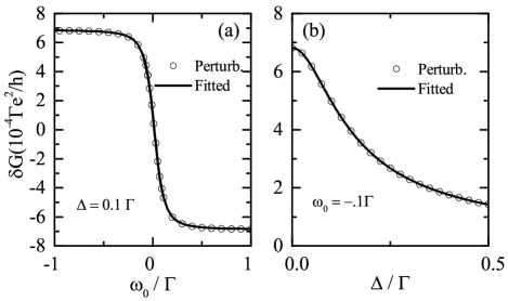
Figure 6: (a) Plot of $\delta G$ as a function of $\omega_{0}$ for $\Delta=.1\Gamma$, (b) Plot of $\delta G$ as a function of $\Delta$ for $\omega_{0}=-.1\Gamma$. Other parameters are $\varepsilon_{d}=-1.2\Gamma$, $V_{b}=.5\Gamma$ and $\lambda=.01\Gamma$. Circles are perturbative results and full lines are fittings to the function $f\left[\omega_{0},\Delta\right]$ with $a=1.6*10^{-2}$ and $c=-6.9*10^{-4}$.

In order to describe the aforementioned dependence of $\delta G$ on $\Delta$ and $\omega_{0}$, we focus on the peaks which are specified in Figs.5(b) and (c) by vertical dashed lines, and plot the calculated values of $\delta G$ with respect to the $\omega_{0}$ and $\Delta$, respectively, in Figs.6(a) and (b). Surprisingly, we see that both numerical data points in Figs.6(a) and (b) are fitted perfectly to the function $f\left[\omega_{0},\Delta\right]=c\left(\omega_{0}-a\right)/\sqrt{\left(\omega_{0}-a\right)^{2}+\Delta^{2}}$. We could intuitively interpret this behavior by the fact that the ground-state expectation value of $\tau_{3}$ for an isolated charge qubit, with the same configuration as in our model system, is equal to $\left\langle\tau_{3}\right\rangle_{isolated}=-\omega_{0}/\sqrt{\omega_{0}^{2}+\Delta^{2}}$. As a result the above functional form for $\delta G$ would be expected to describe correctly the linear relation of $\delta G$ with the ground-state expectation value of $\tau_{3}$ of a charge qubit which is capacitively coupled to the SQD.

From an experimental point of view, the above relation for $\delta G$ suggests a possible indirect measurement of the stationary-state value of $\left\langle\tau_{3}\right\rangle$ by measuring $\delta G$. By setting the value of $\omega_{0}$ to a very large value($\omega_{0}\rightarrow\pm\infty$), the two end points of the lines in the Fig.4 are obtained. Therefore one could find the value of constant $c$ by using the relation $c=\left[\delta G\left(\omega_{0}\gg 0\right)-\delta G\left(\omega_{0}\ll 0\right)\right]/2$. We emphasize the distinction between this measured value for $\left\langle\tau_{3}\right\rangle$ and the initial charge expectation value of the qubit (i.e. its value before the measurement starts). Obviously, because all initial-state informations are washed out by detector during readout process, the stationary-state value of $\left\langle\tau_{3}\right\rangle$ is by no means related to its initial value. Nevertheless, the study of stationary-state properties of a qubit could be still desirable in the sense that one can obtain certain informations about qubit-detector coupled system and use them in performing manipulations or measurements on the qubitmakhlin2001quantum ; averin2001continuous ; korotkov2001output ; ruskov2002quantum ; ruskov2003spectrum ; gurvitz2003relaxation ; gilad2006qubit .

At this point, it is interesting to compare our results for dependence of $\delta G$ curves on $\Delta$ with the results of Ref.hell2014, . In that work, it is claimed that the overall shapes of $\delta G$ would not be altered to the first order in $\Delta$. To show that our results are in accordance at some approximate level with the results of Ref.hell2014, , we could expand the function $\delta G=f\left[\omega_{0},\Delta\right]$ around small values of $\Delta$, then it is revealed that the correspondence between $\delta G$ and $\Delta$ in Fig.5(b) is actually provided through next to the leading order in $\Delta$, i.e. $\delta G_{\Delta\rightarrow 0}\approx c+\mathcal{O}\left(\Delta^{2}\right)$, which is in accord with the above reference.

IV Conclusions

We used the method of non-equilibrium Green’s functions to study the effect of electron-electron interaction between a SQD and a singly occupied DQD(charge qubit) on their static and dynamic properties at zero and finite bias voltages. To this end, we utilized the infinite-U Lacroix approximation and the Majorana fermion representation of spin operators to find the interacting Green’s funcions of the system perturbatively to the second order in the SQD-qubit coupling constant. We calculated the Green’s functions and self-energies of the system in a self-consistent manner with which we could take into account the back-action effects on the system. At zero bias, we checked the accuracy of our results by comparing them with the NRG method. The agreement was good for the density of states of SQD and the expectation value of difference electron occupations of qubit($\left\langle\tau_{3}\right\rangle$). We found a linear relation between the differential conductance of SQD($\delta G$) and stationary-state expectation value of $\left\langle\tau_{3}\right\rangle$. Concerning with this linear relation, we gave NRG results at zero bias, as a support for our perturbative results, from which perfect linear relation was observed. We also investigated the dependency of $\delta G$ on various parameters of the system such as $V_{b}$, $\Delta$, $\omega_{0}$ and $\varepsilon_{d}$. We found that the $\delta G$ curves are best pronounced at zero bias voltage and their amplitudes are decreased relatively by increasing bias voltages. Furthermore, we found an approximate functional form for $\delta G$ with respect to $\Delta$ and $\omega_{0}$. By using this analytical expression, we became able to describe the reason why the authors of Ref.hell2014, stated that the $\delta G$ curves are not dependent on the values of $\Delta$.

Appendix A Expressions for self-energies of SQD and DQD

In this appendix, we give the expressions for self-energies of SQD and DQD, respectively, due to the interaction Hamiltonian $\mathcal{H}_{I}$. The first order self-energies are identically zero for both SQD and DQD because we have taken into account their effect in the non-interacting Green’s functions.

The SQD’s second order self-energies are

$$\Sigma_{d}^{(2nd)R}\left(\omega\right) =\lambda^{2}\int\frac{d\omega_{1}}{2\pi}[g_{d}^{<}\left(\omega\right)\Phi^{R}\left(\omega-\omega_{1}\right)$$

$$+g_{d}^{R}\left(\omega\right)\Phi^{<}\left(\omega-\omega_{1}\right)+g_{d}^{R}\left(\omega\right)\Phi^{R}\left(\omega-\omega_{1}\right)]$$ (27a)

and

$$\Sigma_{d}^{(2nd)<}\left(\omega\right)=\lambda^{2}\int\frac{d\omega_{1}}{2\pi}g_{d}^{<}\left(\omega\right)\Phi^{<}\left(\omega-\omega_{1}\right),$$ (27b)

where

$$\Phi^{R}(\omega)=\int\frac{d\omega_{1}}{2\pi}[ g_{\eta,11}^{<}\left(\omega+\omega_{1}\right)g_{\eta,22}^{A}\left(\omega_{1}\right)+$$

$$g_{\eta,11}^{R}\left(\omega+\omega_{1}\right)g_{\eta,22}^{<}\left(\omega_{1}\right)-$$

$$g_{\eta,12}^{<}\left(\omega+\omega_{1}\right)g_{\eta,21}^{A}\left(\omega_{1}\right)-$$

$$g_{\eta,12}^{R}\left(\omega+\omega_{1}\right)g_{\eta,21}^{<}\left(\omega_{1}\right)]$$ (28a)

and

$$\Phi^{<}(\omega)=\int\frac{d\omega_{1}}{2\pi}[ g_{\eta,11}^{<}\left(\omega+\omega_{1}\right)g_{\eta,22}^{>}\left(\omega_{1}\right)-$$

$$g_{\eta,12}^{<}\left(\omega+\omega_{1}\right)g_{\eta,21}^{>}\left(\omega_{1}\right)].$$ (28b)

For DQD, the second order self-energies are

$$\Sigma_{\eta}^{(2nd)R,<}\left(\omega\right) =\left(\begin{array}[]{ccc}F_{22}^{R,<}\left(\omega\right)&F_{21}^{R,<}\left(\omega\right)&0\\ F_{12}^{R,<}\left(\omega\right)&F_{11}^{R,<}\left(\omega\right)&0\\ 0&0&0\end{array}\right),$$ (32)

where

$$F_{mn}^{R}\left(\omega\right)=\lambda^{2}\underset{\nu=\uparrow,\downarrow}{\sum}\int\frac{d\omega_{1}}{2\pi}[ g_{\eta,mn}^{<}\left(\omega\right)\Pi_{\nu}^{R}(\omega-\omega_{1})+$$

$$g_{\eta,mn}^{R}\left(\omega\right)\Pi_{\nu}^{<}(\omega-\omega_{1})+$$

$$g_{\eta,mn}^{R}\left(\omega\right)\Pi_{\nu}^{R}(\omega-\omega_{1})]$$ (33a)

and

$$F_{mn}^{<}\left(\omega\right)=\lambda^{2}\underset{\nu=\uparrow,\downarrow}{\sum}\int\frac{d\omega_{1}}{2\pi}g_{\eta,mn}^{<}\left(\omega\right)\Pi_{\nu}^{<}(\omega-\omega_{1}).$$ (33b)

In Eqs.(33), the functions $\Pi_{\nu}^{R,<}\left(\omega\right)$ are given by

$$\Pi_{\nu}^{R}(\omega)=\int\frac{d\omega_{1}}{2\pi}[ g_{d,\nu\nu}^{<}\left(\omega+\omega_{1}\right)g_{d,\nu\nu}^{A}\left(\omega_{1}\right)+$$

$$g_{d,\nu\nu}^{R}\left(\omega+\omega_{1}\right)g_{d,\nu\nu}^{<}\left(\omega_{1}\right)]$$ (34a)

and

$$\Pi_{\nu}^{<}(\omega)=\int\frac{d\omega_{1}}{2\pi}g_{d,\nu\nu}^{<}\left(\omega+\omega_{1}\right)g_{d,\nu\nu}^{>}\left(\omega_{1}\right).$$ (34b)

Appendix B Self-consistent calculations

In our numerical results, we have calculated the set of four unknown quantities ($P_{\nu}\left(\omega\right)$, $Q_{\nu}\left(\omega\right)$, $\left\langle n_{d,\nu}\right\rangle$ and $\left\langle\tau_{3}\right\rangle$) by solving self-consistently the Eqs.(10), (23) and (24). This way we assure that the back-action effects are correctly taken into account in the results. We used the following scheme:

($\mathit{i}$) We start with an initial guess for $\left\langle n_{d}\right\rangle$ and $\left\langle\tau_{3}\right\rangle$ and set $P\left(\omega\right)=Q\left(\omega\right)=0$ and then compute $g_{d}^{R}\left(\omega\right)$ from Eq.(9).

($\mathit{i}i$) We calculate $P\left(\omega\right)\text{ and }Q\left(\omega\right)$ from computed $g_{d}^{R}\left(\omega\right)$ and use them to obtain a new $g_{d}^{R}\left(\omega\right)$. We iterate this step until convergence over $g_{d}^{R}\left(\omega\right)$ is attained.

($\mathit{i}ii$) Using the calculated $g_{d}^{R,<}\left(\omega\right)$ and $g_{\eta}^{R,<}\left(\omega\right)$, the self-energies are calculated straightforwardly and then we use the interacting lesser Green’s functions, Eqs.(14) and (22), to calculate new $\left\langle n_{d}\right\rangle$ and $\left\langle\tau_{3}\right\rangle$.

We iterate these three steps until convergence over $\left\langle n_{d}\right\rangle$ and $\left\langle\tau_{3}\right\rangle$ is attained.

Appendix C Analytical expression for $\delta G$

For a SQD with $U=0$, it is possible to obtain an analytical expression for the linear relation between $\delta G$ and $\left\langle\tau_{3}\right\rangle$. To this end, we expand Eq.(26) to the first order in $\lambda$, i.e. $\delta G_{\lambda\rightarrow 0}\approx\lambda\left.\frac{\partial G_{\lambda\neq 0}}{\partial\lambda}\right|_{\lambda=0}$, and then using Eq.(25) and $\mathcal{G}_{d}^{R}\left(\omega\right)=\left[\omega-\varepsilon_{d}-\lambda\left\langle\tau_{3}\right\rangle+i\Gamma-\Sigma_{d}^{(2nd)R}\left(\omega\right)\right]^{-1}$, we obtain

$$\delta G_{\lambda\rightarrow 0}\approx\lambda\underset{V=\pm\frac{V_{b}}{2}}{\sum}\left(\frac{\Gamma(\varepsilon_{d}+V)}{\pi\left(\left(\varepsilon_{d}+V\right)^{2}+\Gamma^{2}\right)^{2}}\right)\left\langle\tau_{3}\right\rangle+\mathcal{O}\left(\lambda^{2}\right).$$

One immediate consequence of this expression is that even at the zero bias voltage there would be an obvious conductance difference in the system, i.e. $\delta G_{V_{b}=0}\approx\lambda\frac{2\Gamma\varepsilon_{d}}{\pi\left(\varepsilon_{d}^{2}+\Gamma^{2}\right)^{2}}\left\langle\tau_{3}\right\rangle+\mathcal{O}\left(\lambda^{2}\right)$.

References

- [1] IL Aleiner, Ned S Wingreen, and Yigal Meir. Dephasing and the orthogonality catastrophe in tunneling through a quantum dot. Physical Review Letters, 79(19):3740, 1997.
- [2] Shmuel A Gurvitz. Measurements with a noninvasive detector and dephasing mechanism. Physical Review B, 56(23):15215, 1997.
- [3] JM Elzerman, R Hanson, LH Willems Van Beveren, B Witkamp, LMK Vandersypen, and Leo P Kouwenhoven. Single-shot read-out of an individual electron spin in a quantum dot. nature, 430(6998):431–435, 2004.
- [4] AN Korotkov and DV Averin. Continuous weak measurement of quantum coherent oscillations. Physical Review B, 64(16):165310, 2001.
- [5] Hsi-Sheng Goan, Gerard J Milburn, Howard Mark Wiseman, and He Bi Sun. Continuous quantum measurement of two coupled quantum dots using a point contact: A quantum trajectory approach. Physical Review B, 63(12):125326, 2001.
- [6] TM Stace and SD Barrett. Continuous quantum measurement: Inelastic tunneling and lack of current oscillations. Physical review letters, 92(13):136802, 2004.
- [7] Hans-Andreas Engel, Vitaly N Golovach, Daniel Loss, LMK Vandersypen, JM Elzerman, R Hanson, and LP Kouwenhoven. Measurement efficiency and n-shot readout of spin qubits. Physical review letters, 93(10):106804, 2004.
- [8] JunYan Luo, HuJun Jiao, BiTao Xiong, Xiao-Ling He, and Changrong Wang. Non-markovian dynamics and noise characteristics in continuous measurement of a solid-state charge qubit. Journal of Applied Physics, 114(17):173703, 2013.
- [9] RJ Schoelkopf, P Wahlgren, AA Kozhevnikov, P Delsing, and DE Prober. The radio-frequency single-electron transistor (rf-set): a fast and ultrasensitive electrometer. Science, 280(5367):1238–1242, 1998.
- [10] Yu Nakamura, Yu A Pashkin, and JS Tsai. Coherent control of macroscopic quantum states in a single-cooper-pair box. Nature, 398(6730):786–788, 1999.
- [11] Abdel Aassime, Goeran Johansson, Goeran Wendin, RJ Schoelkopf, and P Delsing. Radio-frequency single-electron transistor as readout device for qubits: charge sensitivity and backaction. Physical Review Letters, 86(15):3376, 2001.
- [12] Wei Lu, Zhongqing Ji, Loren Pfeiffer, KW West, and AJ Rimberg. Real-time detection of electron tunnelling in a quantum dot. Nature, 423(6938):422–425, 2003.
- [13] O Astafiev, Yu A Pashkin, T Yamamoto, Y Nakamura, and JS Tsai. Single-shot measurement of the josephson charge qubit. Physical Review B, 69(18):180507, 2004.
- [14] MD LaHaye, Olivier Buu, Benedetta Camarota, and KC Schwab. Approaching the quantum limit of a nanomechanical resonator. Science, 304(5667):74–77, 2004.
- [15] BA Turek, KW Lehnert, A Clerk, David Gunnarsson, Kevin Bladh, Per Delsing, and RJ Schoelkopf. Single-electron transistor backaction on the single-electron box. Physical Review B, 71(19):193304, 2005.
- [16] C. Barthel, M. Kjærgaard, J. Medford, M. Stopa, C. M. Marcus, M. P. Hanson, and A. C. Gossard. Fast sensing of double-dot charge arrangement and spin state with a radio-frequency sensor quantum dot. Phys. Rev. B, 81:161308, Apr 2010.
- [17] AB Zorin, F-J Ahlers, J Niemeyer, Th Weimann, H Wolf, VA Krupenin, and SV Lotkhov. Background charge noise in metallic single-electron tunneling devices. Physical Review B, 53(20):13682, 1996.
- [18] Alex Grishin, Igor V Yurkevich, and Igor V Lerner. Low-temperature decoherence of qubit coupled to background charges. Physical Review B, 72(6):060509, 2005.
- [19] Yuriy Makhlin, Gerd Schön, and Alexander Shnirman. Quantum-state engineering with josephson-junction devices. Reviews of modern physics, 73(2):357, 2001.
- [20] D. Sprinzak, E. Buks, M. Heiblum, and H. Shtrikman. Controlled dephasing of electrons via a phase sensitive detector. Phys. Rev. Lett., 84:5820–5823, Jun 2000.
- [21] Yuriy Makhlin, Gerd Schön, and Alexander Shnirman. Statistics and noise in a quantum measurement process. Physical review letters, 85(21):4578, 2000.
- [22] Alexander N Korotkov. Selective quantum evolution of a qubit state due to continuous measurement. Physical Review B, 63(11):115403, 2001.
- [23] SA Gurvitz and GP Berman. Single qubit measurements with an asymmetric single-electron transistor. Physical Review B, 72(7):073303, 2005.
- [24] SA Gurvitz and D Mozyrsky. Quantum mechanical approach to decoherence and relaxation generated by fluctuating environment. Physical Review B, 77(7):075325, 2008.
- [25] Alexander Shnirman and Gerd Schoen. Quantum measurements performed with a single-electron transistor. Physical Review B, 57(24):15400, 1998.
- [26] D Mozyrsky, I Martin, and MB Hastings. Quantum-limited sensitivity of single-electron-transistor-based displacement detectors. Physical review letters, 92(1):018303, 2004.
- [27] Neil P Oxtoby, Howard Mark Wiseman, and He-Bi Sun. Sensitivity and back action in charge qubit measurements by a strongly coupled single-electron transistor. Physical Review B, 74(4):045328, 2006.
- [28] Clive Emary. Quantum dynamics in nonequilibrium environments. Physical Review A, 78(3):032105, 2008.
- [29] Jens Schulenborg, Janine Splettstoesser, Michele Governale, and L Debora Contreras-Pulido. Detection of the relaxation rates of an interacting quantum dot by a capacitively coupled sensor dot. Physical Review B, 89(19):195305, 2014.
- [30] M. Hell, M. R. Wegewijs, and D. P. DiVincenzo. Coherent backaction of quantum dot detectors: Qubit isospin precession. Phys. Rev. B, 89:195405, May 2014.
- [31] M Hell, MR Wegewijs, and DP DiVincenzo. Qubit quantum-dot sensors: Noise cancellation by coherent backaction, initial slips, and elliptical precession. Physical Review B, 93(4):045418, 2016.
- [32] AM Tsvelik. New fermionic description of quantum spin liquid state. Physical review letters, 69(14):2142, 1992.
- [33] W Mao, P Coleman, C Hooley, and D Langreth. Spin dynamics from majorana fermions. Physical review letters, 91(20):207203, 2003.
- [34] Alexander Shnirman and Yuriy Makhlin. Spin-spin correlators in the majorana representation. Physical review letters, 91(20):207204, 2003.
- [35] C Lacroix. Density of states for the anderson model. Journal of Physics F: Metal Physics, 11(11):2389, 1981.
- [36] Ralf Bulla, Theo A Costi, and Thomas Pruschke. Numerical renormalization group method for quantum impurity systems. Reviews of Modern Physics, 80(2):395, 2008.
- [37] Heinz-Peter Breuer and Francesco Petruccione. The theory of open quantum systems. Oxford University Press on Demand, 2002.
- [38] J Gorman, DG Hasko, and DA Williams. Charge-qubit operation of an isolated double quantum dot. Physical review letters, 95(9):090502, 2005.
- [39] Gianluca Stefanucci and Robert van Leeuwen. Nonequilibrium Many-Body Theory of Quantum Systems: A Modern Introduction. Cambridge University Press, 2013.
- [40] Raphaël Van Roermund, Shiue-yuan Shiau, and Mireille Lavagna. Anderson model out of equilibrium: Decoherence effects in transport through a quantum dot. Phys. Rev. B, 81:165115, Apr 2010.
- [41] Tai-Kai Ng. ac response in the nonequilibrium anderson impurity model. Phys. Rev. Lett., 76:487–490, Jan 1996.
- [42] J. R. Petta, A. C. Johnson, C. M. Marcus, M. P. Hanson, and A. C. Gossard. Manipulation of a single charge in a double quantum dot. Phys. Rev. Lett., 93:186802, Oct 2004.
- [43] R.Zitko. The package is available at http://nrgljubljana.ijs.si.
- [44] DV Averin. Continuous weak measurement of the macroscopic quantum coherent oscillations of magnetic flux. Physica C: Superconductivity, 352(1):120–124, 2001.
- [45] Alexander N Korotkov. Output spectrum of a detector measuring quantum oscillations. Physical Review B, 63(8):085312, 2001.
- [46] Rusko Ruskov and Alexander N Korotkov. Quantum feedback control of a solid-state qubit. Physical Review B, 66(4):041401, 2002.
- [47] Rusko Ruskov and Alexander N Korotkov. Spectrum of qubit oscillations from generalized bloch equations. Physical Review B, 67(7):075303, 2003.
- [48] Shmuel A Gurvitz, Leonid Fedichkin, Dima Mozyrsky, and Gennady P Berman. Relaxation and the zeno effect in qubit measurements. Physical review letters, 91(6):066801, 2003.
- [49] T Gilad and SA Gurvitz. Qubit measurements with a double-dot detector. Physical review letters, 97(11):116806, 2006.