Numerical algorithm for two-dimensional time-fractional wave equation of distributed-order with a nonlinear source term

Abstract

In this paper, an alternating direction implicit (ADI) difference scheme for two-dimensional time-fractional wave equation of distributed-order with a nonlinear source term is presented. The unique solvability of the difference solution is discussed, and the unconditional stability and convergence order of the numerical scheme are analysed. Finally, numerical experiments are carried out to verify the effectiveness and accuracy of the algorithm.

1 Introduction

The idea of distributed-order differential equation was first introduced by Caputo in his work for modeling the stress-strain behavior of an anelastic medium in 1960s [1]. Being different from the differential equations with the single-order fractional derivative and the ones with sums of fractional derivatives, i.e., multi-term fractional differential equations (FDEs), the distributed-order differential equations are derived by integrating the order of differentiation over a certain range. It can be regarded as a generalization of the aforementioned two classes of FDEs. A typical application of this kind of FDEs is in the retarding sub-diffusion process, where a plume of particles spreads at a logarithmic rate, which leads to ultraslow diffusion (see [2][3][4]). Another example is the fractional Langevin equation of distributed-order, which was proposed to model the kinetics of retarding sub-diffusion whose scaling exponent decreases in time, and then was applied to simulate the strongly anomalous ultraslow diffusion with the mean square displacement growing as a power of logarithm of time [5]. The distributed-order FDEs were also found playing important role in other various research fields, such as control and signal processing [6], modelling dielectric induction and diffusion [7], identification of systems [8], and so on.

Till now, there have been many important progresses for the research on analytical solutions of distributed-order FDEs. For the kinetic description of anomalous diffusion and relaxation phenomena, A. V. Chechkin et al. presented the diffusion-like equation with time fractional derivative of distributed-order in [9], where the positivity of the solutions of the proposed equation was proved and the relation to the continuous-time random walk theory was established. T. M. Atanackovic et al. analysed a Cauchy problem for a time distributed-order diffusion-wave equation by means of the theory of an abstract Volterra equation [10]. In [11], for the one-dimensional distributed-order diffusion-wave equation, R. Gorenflo et al. gave the interpretation of the fundamental solution of the Cauchy problem as a probability density function of the space variable $x$ evolving in time $t$ in the transform domain by employing the technique of the Fourier and Laplace transforms. Using the Laplace transform method, Z. Li et al investigated the asymptotic behavior of solutions to the initial-boundary-value problem for the distributed-order time-fractional diffusion equations [12].

In most instances, the analytical solutions of distributed-order differential equations are not easy to available, thus it stimulates researchers to develop numerical algorithms for approximate solutions. To our knowledge, the research on numerically solving the distributed-order differential equations are still in its infancy. The literatures [13][14][15] concerned on developing numerical methods for solving distributed-order ordinary differential equations. In terms of the distributed-order partial differential equations, most of the work are about the one-dimensional time distributed-order differential equations, and the integrating range of the order of time derivative is the interval $[0,1]$, which is named as time distributed-order diffusion equation. N. J. Ford et al. developed an implicit finite difference method for the solution of the diffusion equation with distributed order in time [16]. By using the Grünwald-Letnikov formula, Gao et al. proposed two difference schemes to solve the one-dimensional distributed-order differential equations, and the extrapolation method was applied to improve the approximate accuracy [17]. In [18], the authors handled the same distributed-order differential equations by employing a weighted and shifted Grünwald-Letnikov formula to derive several second-order convergent difference schemes. When the order of the time derivative is distributed over the interval $[1,2]$, it is called the time distributed-order wave equation. The study of the numerical solution of this kind of equation is rather more limited. Ye et al. derived and analysed a compact difference scheme for a distributed-order time-fractional wave equation in [19].

When considering the high-dimensional models, Gao et al. investigated ADI schemes for two-dimensional distributed-order diffusion equations [20][21], and they also developed two ADI difference schemes for solving the two-dimensional time distributed-order wave equations [22]. Due to the widespread use of the nonlinear models [23][24], M. L. Morgado et al. developed an implicit difference scheme for one-dimensional time distributed-order diffusion equation with a nonlinear source term [25]. For further discussion on the numerical approaches for solving the high-dimensional distributed-order partial differential equations, this paper is devoted to develop effective numerical algorithm for two-dimensional time-fractional wave equation of distributed-order with a nonlinear source term

$$\int_{1}^{2}p(\beta){}_{0}^{C}D_{t}^{\beta}u(x,y,t)d\beta=\frac{\partial^{2}u(x,y,t)}{\partial x^{2}}+\frac{\partial^{2}u(x,y,t)}{\partial x^{2}}+f\big{(}x,y,t,u(x,y,t)\big{)},$$

$$(x,y)\in\Omega,\quad t\in(0,T],$$ (1.1)

$$u(x,y,t)=\phi(x,y,t),\quad(x,y)\in\partial\Omega,\quad 0\leq t<T,$$ (1.2)

$$u(x,y,0)=\psi_{1}(x,y),\quad u_{t}(x,y,0)=\psi_{2}(x,y),\quad(x,y)\in\Omega,$$ (1.3)

where $\Omega=(0,L_{1})\times(0,L_{2})$, and $\partial\Omega$ is the boundary of $\Omega$. The fractional derivative ${}_{0}^{C}D_{t}^{\beta}v(t)$ in (1) is given in the Caputo sense

$${}_{0}^{C}D_{t}^{\beta}v(t)=\left\{\begin{aligned} &\frac{\partial v(t)}{\partial t}-\frac{\partial v(0)}{\partial t},\ \beta=1,\\ &\frac{1}{\Gamma{(2-\beta)}}\int_{0}^{t}(t-\xi)^{1-\beta}\frac{\partial^{2}v(\xi)}{\partial\xi^{2}}d\xi,\ 1<\beta<2,\\ &\frac{\partial^{2}v(t)}{\partial t^{2}},\ \beta=2,\end{aligned}\right.$$

and the function $p(\beta)$ is served as weight for the order of differentiation such that $p(\beta)>0$ and $\int_{1}^{2}p(\beta)d\beta=c_{0}>0$. We assume that $p(\beta)$, $\phi(x,y,t)$, $\psi_{1}(x,y)$, $\psi_{2}(x,y)$ and $f(x,y,t,u)$ are continuous, and the nonlinear source term $f$ satisfies a Lipschitz condition of the form

$$|f(x,y,t,u_{1})-f(x,y,t,u_{2})|\leq L_{f}|u_{1}-u_{2}|,$$ (1.4)

where $L_{f}$ is a positive constant.

The main procedure of developing numerical scheme for solving problem (1)$-$(1.3) is as follows. Firstly a suitable numerical quadrature formula is adopted to discrete the integral in (1), and a multi-term time fractional wave equation is left whereafter. Then we develop an ADI finite difference scheme which is uniquely solvable for the multi-term time fractional wave equation. By using the discrete energy method, we prove the derived numerical scheme is unconditionally stable and convergent.

The rest of this paper is organized in the following way. In Section 2, the ADI finite difference scheme is constructed and described detailedly. In Section 3, we give analysis on solvability, stability and convergence for the derived difference scheme. Numerical results are illustrated in Section 4 to confirm the effectiveness and accuracy of our method, and some conclusions are drawn in the last section.

2 The derivation of the ADI scheme

This section focuses on deriving the ADI scheme for the problems (1)$-$(1.3).

Let ${M_{1}}$, ${M_{2}}$ and $N$ be positive integers, and $h_{1}=L_{1}/M_{1}$, $h_{2}=L_{2}/M_{2}$ and $\tau=T/N$ be the uniform sizes of spatial grid and time step, respectively. Then a spatial and temporal partition can be defined as $x_{i}=ih_{1}$ for $i=0,1,\cdots,M_{1}$, $y_{j}=jh_{2}$ for $j=0,1,\cdots,M_{2}$ and $t_{n}=n\tau$ for $n=0,1,\cdots,N$. Denote $\bar{\Omega}_{h}=\{(x_{i},y_{j})\mid 0\leq i\leq M_{1},0\leq j\leq M_{2}\}$ and $\Omega_{\tau}=\{t_{n}\mid t_{n}=n\tau,0\leq n\leq N\}$, then the domain $\bar{\Omega}\times[0,T]$ is covered by $\bar{\Omega}_{h}\times\Omega_{\tau}$. Let $u=\{u_{ij}^{n}\mid 0\leq i\leq M_{1},0\leq j\leq M_{2},0\leq n\leq N\}$ be a grid function on $\bar{\Omega}_{h}\times\Omega_{\tau}$. We introduce the following notations:

$$u_{ij}^{n-\frac{1}{2}}=\frac{1}{2}(u_{ij}^{n}+u_{ij}^{n-1}),\qquad\delta_{t}u_{ij}^{n-\frac{1}{2}}=\frac{1}{\tau}(u_{ij}^{n}-u_{ij}^{n-1}),$$

$$\delta_{x}u_{i-\frac{1}{2},j}^{n}=\frac{1}{h_{1}}(u_{ij}^{n}-u_{i-1,j}^{n}),\qquad\delta_{x}^{2}u_{ij}^{n}=\frac{1}{h_{1}}(\delta_{x}u_{i+\frac{1}{2},j}^{n}-\delta_{x}u_{i-\frac{1}{2},j}^{n}),$$

$$\delta_{y}u_{i,j-\frac{1}{2}}^{n}=\frac{1}{h_{2}}(u_{ij}^{n}-u_{i,j-1}^{n}),\qquad\delta_{y}^{2}u_{ij}^{n}=\frac{1}{h_{2}}(\delta_{x}u_{i,j+\frac{1}{2}}^{n}-\delta_{x}u_{i,j-\frac{1}{2}}^{n}),$$

and

$$\Delta_{h}u_{ij}=\delta_{x}^{2}u_{ij}+\delta_{y}^{2}u_{ij}.$$

Consider Eq. (1) at the point $(x_{i},y_{j},t_{n})$, and we write it as

$$\int_{1}^{2}p(\beta){}_{0}^{C}D_{t}^{\beta}u(x_{i},y_{j},t_{n})d\beta$$ (2.1)

$$= \frac{\partial^{2}u(x_{i},y_{j},t_{n})}{\partial x^{2}}+\frac{\partial^{2}u(x_{i},y_{j},t_{n})}{\partial y^{2}}+f\big{(}x_{i},y_{j},t_{n},u(x_{i},y_{j},t_{n})\big{)}.$$

Take an average of Eq. (2.1) on time level $t=t_{n}$ and $t=t_{n-1}$, then we have

$$\frac{1}{2}\bigg{(}\int_{1}^{2}p(\beta){}_{0}^{C}D_{t}^{\beta}u(x_{i},y_{j},t_{n})d\beta+\int_{1}^{2}p(\beta){}_{0}^{C}D_{t}^{\beta}u(x_{i},y_{j},t_{n-1})d\beta\bigg{)}$$ (2.2)

$$= \frac{1}{2}\bigg{[}\frac{\partial^{2}u(x_{i},y_{j},t_{n})}{\partial x^{2}}+\frac{\partial^{2}u(x_{i},y_{j},t_{n-1})}{\partial x^{2}}\bigg{]}+\frac{1}{2}\bigg{[}\frac{\partial^{2}u(x_{i},y_{j},t_{n})}{\partial y^{2}}+\frac{\partial^{2}u(x_{i},y_{j},t_{n-1})}{\partial y^{2}}\bigg{]}$$

$$+\frac{1}{2}\bigg{[}f\big{(}x_{i},y_{j},t_{n},u(x_{i},y_{j},t_{n})\big{)}+f\big{(}x_{i},y_{j},t_{n-1},u(x_{i},y_{j},t_{n-1})\big{)}\bigg{]}.$$

Denote by $U_{ij}^{n}=u(x_{i},y_{j},t_{n})$ the grid functions on $\bar{\Omega}_{h}\times\Omega_{\tau}$ with $0\leq i\leq M_{1}$, $0\leq j\leq M_{2}$, $0\leq n\leq N$. Eq. (2.2) can be expressed as

$$\int_{1}^{2}p(\beta){}_{0}^{C}D_{t}^{\beta}U_{ij}^{n-\frac{1}{2}}d\beta= \frac{\partial^{2}}{\partial x^{2}}U_{ij}^{n-\frac{1}{2}}+\frac{\partial^{2}}{\partial y^{2}}U_{ij}^{n-\frac{1}{2}}$$ (2.3)

$$+\frac{1}{2}\bigg{[}f\big{(}x_{i},y_{j},t_{n},U_{ij}^{n}\big{)}+f\big{(}x_{i},y_{j},t_{n-1},U_{ij}^{n-1}\big{)}\bigg{]}$$

Firstly we discretize the integral term in (2.3). Suppose $p(\beta)\in C^{2}[1,2]$, ${}_{0}^{C}D_{t}^{\beta}u(x_{i},y_{j},t)|_{t=t_{n-1}}$ and ${}_{0}^{C}D_{t}^{\beta}u(x_{i},y_{j},t)|_{t=t_{n}}\in C^{2}[1,2]$. Let $K$ be a positive integer, and $\Delta\beta=1/K$ be the uniform step size. Take $\beta_{l}=1+\frac{2l-1}{2}\Delta\beta$, $1\leq l\leq K$, then the mid-point quadrature rule is used for approximating the integral in (2.3)

$$\Delta\beta\sum_{l=1}^{K}p(\beta_{l}){}_{0}^{C}D_{t}^{\beta_{l}}U_{ij}^{n-\frac{1}{2}}+R_{1}=\frac{\partial^{2}}{\partial x^{2}}U_{ij}^{n-\frac{1}{2}}+\frac{\partial^{2}}{\partial y^{2}}U_{ij}^{n-\frac{1}{2}}$$ (2.4)

$$+\frac{1}{2}\bigg{[}f\big{(}x_{i},y_{j},t_{n},U(x_{i},y_{j},t_{n})\big{)}+f\big{(}x_{i},y_{j},t_{n-1},U(x_{i},y_{j},t_{n-1})\big{)}\bigg{]},$$

where $R_{1}=\mathcal{O}(\Delta\beta^{2})$.

Next, we solve the multi-term time fractional wave equation (2.4) with the initial and boundary conditions (1.3) and (1.2). Suppose $u(x,y,t)\in C_{x,y,t}^{4,4,3}(\bar{\Omega}\times[0,T])$. According to Theorem 8.2.5 in [26], the Caputo derivative ${}_{0}^{C}D_{t}^{\beta_{l}}U_{ij}^{n-\frac{1}{2}}$, $1<\beta_{l}<2$ have the fully discrete difference scheme

$${}_{0}^{C}D_{t}^{\beta_{l}}U_{ij}^{n-\frac{1}{2}}$$ (2.5)

$$= \frac{\tau^{1-\beta_{l}}}{\Gamma(3-\beta_{l})}\bigg{[}a_{0}^{(\beta_{l})}\delta_{t}U_{ij}^{n-\frac{1}{2}}-\sum_{k=1}^{n-1}\big{(}a_{n-k-1}^{(\beta_{l})}-a_{n-k}^{(\beta_{l})}\big{)}\delta_{t}U_{ij}^{k-\frac{1}{2}}-a_{n-1}^{(\beta_{l})}\psi_{2}(x_{i},y_{j})\bigg{]}+R_{2}^{l},$$

where

$$a_{k}^{(\beta_{l})}=(k+1)^{2-\beta_{l}}-k^{2-\beta_{l}},\quad k=0,1,2,\cdots,$$

and

$$\mid R_{2}^{l}\mid\leq \frac{1}{\Gamma(3-\beta_{l})}\bigg{[}\frac{2-\beta_{l}}{12}+\frac{2^{3-\beta_{l}}}{3-\beta_{l}}-(1+2^{1-\beta_{l}})+\frac{1}{12}\bigg{]}\cdot$$ (2.6)

$$\max_{0\leq t\leq t_{n}}\mid\frac{\partial^{3}u(x_{i},y_{j},t)}{\partial t^{3}}\mid\tau^{3-\beta_{l}},\quad l=1,2,\cdots,K.$$

In the meantime, using the second order finite difference

$$\frac{\partial^{2}g(x_{i})}{\partial x^{2}}=\frac{g(x_{i+1})-2g(x_{i})+g(x_{i-1})}{(\Delta x)^{2}}-\frac{(\Delta x)^{2}}{12}\frac{\partial^{4}g(\xi_{i})}{\partial x^{4}},\quad\xi_{i}\in(x_{i-1},x_{i+1})$$

to approximate the second order derivatives in (2.4), it is obtained

$$\Delta\beta\sum_{l=1}^{K}p(\beta_{l})\frac{\tau^{1-\beta_{l}}}{\Gamma(3-\beta_{l})}\bigg{[}a_{0}^{(\beta_{l})}\delta_{t}U_{ij}^{n-\frac{1}{2}}-\sum_{k=1}^{n-1}\big{(}a_{n-k-1}^{(\beta_{l})}-a_{n-k}^{(\beta_{l})}\big{)}\delta_{t}U_{ij}^{k-\frac{1}{2}}$$ (2.7)

$$-a_{n-1}^{(\beta_{l})}\psi_{2}(x_{i},y_{j})\bigg{]}+\sum_{l=1}^{K}\Delta\beta p(\beta_{l})R_{2}^{l}+R_{1}$$

$$= \delta_{x}^{2}U_{ij}^{n-\frac{1}{2}}+\delta_{y}^{2}U_{ij}^{n-\frac{1}{2}}+\frac{1}{2}\Big{(}f\big{(}x_{i},y_{j},t_{n-1},U_{ij}^{n-1}\big{)}+f\big{(}x_{i},y_{j},t_{n},U_{ij}^{n}\big{)}\Big{)}+R_{3},$$

where $R_{3}=\mathcal{O}(h_{1}^{2}+h_{2}^{2})$. Subsequently, the nonlinear source term is dealt with in the following manner to avoid a system of nonlinear equations when computing:

$$f(x_{i},y_{j},t_{n},U_{ij}^{n})=f(x_{i},y_{j},t_{n-1},U_{ij}^{n-1})+\mathcal{O}(\tau).$$ (2.8)

Substituting (2.8) in (2.7), we are left with

$$\Delta\beta\sum_{l=1}^{K}p(\beta_{l})\frac{\tau^{1-\beta_{l}}}{\Gamma(3-\beta_{l})}\bigg{[}a_{0}^{(\beta_{l})}\delta_{t}U_{ij}^{n-\frac{1}{2}}-\sum_{k=1}^{n-1}\big{(}a_{n-k-1}^{(\beta_{l})}-a_{n-k}^{(\beta_{l})}\big{)}\delta_{t}U_{ij}^{k-\frac{1}{2}}-a_{n-1}^{(\beta_{l})}\psi_{2}(x_{i},y_{j})\bigg{]}$$ (2.9)

$$=\delta_{x}^{2}U_{ij}^{n-\frac{1}{2}}+\delta_{y}^{2}U_{ij}^{n-\frac{1}{2}}+f\big{(}x_{i},y_{j},t_{n-1},U_{ij}^{n-1}\big{)}+R_{ij}^{n-\frac{1}{2}}+\widetilde{R}_{ij}^{n-\frac{1}{2}},$$

where

$$R_{ij}^{n-\frac{1}{2}}=-\sum_{l=1}^{K}\Delta\beta p(\beta_{l})R_{2}^{l}+\mathcal{O}(h_{1}^{2}+h_{2}^{2})+\mathcal{O}(\Delta\beta^{2})$$

and

$$\widetilde{R}_{ij}^{n-\frac{1}{2}}=\mathcal{O}(\tau).$$

From (2.6), we can deduce that there exists a positive constant $C_{1}$ such that

$$\bigg{|}-\sum_{l=1}^{K}\Delta\beta p(\beta_{l})R_{2}^{l}\bigg{|}\leq C_{1}\tau^{1+\frac{1}{2}\Delta\beta}\sum_{l=1}^{K}\Delta\beta p(\beta_{l}).$$

Since

$$\sum_{l=1}^{K}\Delta\beta p(\beta_{l})\sim\int_{1}^{2}p(\beta)d\beta=c_{0},$$

we get

$$\sum_{l=1}^{K}\Delta\beta p(\beta_{l})\leq C_{2},$$

where $C_{2}$ is a positive constant. Thus there exists a positive constant $C_{3}$ such that

$$\Big{|}R_{ij}^{n-\frac{1}{2}}\Big{|}\leq C_{3}\left(\tau^{1+\frac{1}{2}\Delta\beta}+h_{1}^{2}+h_{2}^{2}+\Delta\beta^{2}\right).$$

Besides, it is obvious that

$$\Big{|}\widetilde{R}_{ij}^{n-\frac{1}{2}}\Big{|}\leq C_{4}\tau,$$

where $C_{4}$ is a positive constant.

Denote

$$\mu=\Delta\beta\sum_{l=1}^{K}p(\beta_{l})\frac{1}{\tau^{\beta_{l}}\Gamma(3-\beta_{l})}.$$

Since

$$\Delta\beta\sum_{l=1}^{K}p(\beta_{l})\frac{1}{\tau^{\beta_{l}}\Gamma(3-\beta_{l})}$$

$$\sim \int_{1}^{2}p(\beta)\frac{1}{\tau^{\beta}\Gamma(3-\beta)}d\beta$$

$$= \frac{p(\beta^{\ast})}{\Gamma(3-\beta^{\ast})}\int_{1}^{2}\frac{1}{\tau^{\beta}}d\beta$$

$$= \frac{p(\beta^{\ast})}{\Gamma(3-\beta^{\ast})}\frac{1-\tau}{\tau^{2}\mid\ln\tau\mid},$$

it can be concluded that

$$\mu=\frac{1}{\mathcal{O}(\tau^{2}|\ln\tau|)}.$$

In addition, $|\ln\tau|\leq C\tau^{-\varepsilon}$ for any positive and small $\varepsilon$ when $\tau$ is sufficiently small, thus the term $\mathcal{O}(\tau^{2}|\ln\tau|)$ is almost the same as $\mathcal{O}(\tau^{2})$ when $\tau$ is sufficiently small. Adding the high order term

$$\frac{\tau}{4\mu}\delta_{x}^{2}\delta_{y}^{2}\frac{U_{ij}^{n}-U_{ij}^{n-1}}{\tau}$$

on both sides of (2.9), we derive

$$\Delta\beta\sum_{l=1}^{K}p(\beta_{l})\frac{\tau^{1-\beta_{l}}}{\Gamma(3-\beta_{l})}\bigg{[}a_{0}^{(\beta_{l})}\delta_{t}U_{ij}^{n-\frac{1}{2}}-\sum_{k=1}^{n-1}\big{(}a_{n-k-1}^{(\beta_{l})}-a_{n-k}^{(\beta_{l})}\big{)}\delta_{t}U_{ij}^{k-\frac{1}{2}}-a_{n-1}^{(\beta_{l})}\psi_{2}(x_{i},y_{j})\bigg{]}$$ (2.10)

$$+\frac{\tau}{4\mu}\delta_{x}^{2}\delta_{y}^{2}\frac{U_{ij}^{n}-U_{ij}^{n-1}}{\tau}$$

$$= \delta_{x}^{2}U_{ij}^{n-\frac{1}{2}}+\delta_{y}^{2}U_{ij}^{n-\frac{1}{2}}+f\big{(}x_{i},y_{j},t_{n-1},U_{ij}^{n-1}\big{)}+R_{ij}^{n-\frac{1}{2}}+\widetilde{R}_{ij}^{n-\frac{1}{2}}+\widehat{R}_{ij}^{n-\frac{1}{2}},$$

where

$$\widehat{R}_{ij}^{n-\frac{1}{2}}=\frac{\tau}{4\mu}\delta_{x}^{2}\delta_{y}^{2}\frac{U_{ij}^{n}-U_{ij}^{n-1}}{\tau},$$

and it is clear that

$$\Big{|}\widehat{R}_{ij}^{n-\frac{1}{2}}\Big{|}\leq C_{5}\tau^{3}|\ln\tau|.$$

Also, for the initial and boundary value conditions, we have

$$U_{ij}^{0}=\psi_{1}(x_{i},y_{j}),\ (x_{i},y_{j})\in\Omega,$$ (2.11)

$$U_{ij}^{n}=\phi(x_{i},y_{j},t_{n}),\ (x_{i},y_{j})\in\partial\Omega,\ 0\leq n\leq N.$$ (2.12)

Let $u_{ij}^{n}$ be the numerical approximation to $u(x_{i},y_{j},t_{n})$. Neglecting the small term $R_{ij}^{n-\frac{1}{2}}$, $\widetilde{R}_{ij}^{n-\frac{1}{2}}$ and $\widehat{R}_{ij}^{n-\frac{1}{2}}$ in (2.10), and using $u_{ij}^{n}$ instead of $U_{ij}^{n}$ in (2.10)$-$(2.12), we construct the difference scheme for (1)$-$(1.3) as follows:

$$\Delta\beta\sum_{l=1}^{K}p(\beta_{l})\frac{\tau^{1-\beta_{l}}}{\Gamma(3-\beta_{l})}\bigg{[}a_{0}^{(\beta_{l})}\delta_{t}u_{ij}^{n-\frac{1}{2}}-\sum_{k=1}^{n-1}\big{(}a_{n-k-1}^{(\beta_{l})}-a_{n-k}^{(\beta_{l})}\big{)}\delta_{t}u_{ij}^{k-\frac{1}{2}}$$

$$-a_{n-1}^{(\beta_{l})}(\psi_{2})_{ij}\bigg{]}+\frac{\tau}{4\mu}\delta_{x}^{2}\delta_{y}^{2}\frac{u_{ij}^{n}-u_{ij}^{n-1}}{\tau}$$

$$= \delta_{x}^{2}u_{ij}^{n-\frac{1}{2}}+\delta_{y}^{2}u_{ij}^{n-\frac{1}{2}}+f\big{(}x_{i},y_{j},t_{n-1},u_{ij}^{n-1}\big{)},$$

$$1\leq i\leq M_{1}-1,\ 1\leq j\leq M_{2}-1,\ 1\leq n\leq N,$$ (2.13)

$$u_{ij}^{0}=(\psi_{1})_{ij},\ 1\leq i\leq M_{1}-1,\ 1\leq j\leq M_{2}-1,$$ (2.14)

$$u_{ij}^{n}=\phi_{ij}^{n},\ (i,j)\in\gamma=\big{\{}(i,j)\ |\ (x_{i},y_{j})\in\partial\Omega\big{\}},\ 0\leq n\leq N,$$ (2.15)

where

$$(\psi_{1})_{ij}=\psi_{1}(x_{i},y_{j}),\ (\psi_{2})_{ij}=\psi_{2}(x_{i},y_{j}),\ 1\leq i\leq M_{1}-1,\ 1\leq j\leq M_{2}-1,$$

and

$$\phi_{ij}^{n}=\phi(x_{i},y_{j},t_{n}),\quad(i,j)\in\gamma,\quad 0\leq n\leq N.$$

Notice $a_{0}^{(\beta_{l})}=1$, then Eq. (2) can be rewritten as:

$$\Delta\beta\sum_{l=1}^{K}p(\beta_{l})\frac{1}{\tau^{\beta_{l}}\Gamma{(3-\beta_{l})}}u_{ij}^{n}-\frac{1}{2}\delta_{x}^{2}u_{ij}^{n}-\frac{1}{2}\delta_{y}^{2}u_{ij}^{n}+\frac{1}{4\mu}\delta_{x}^{2}\delta_{y}^{2}u_{ij}^{n}$$

$$= \Delta\beta\sum_{l=1}^{K}p(\beta_{l})\frac{1}{\tau^{\beta_{l}}\Gamma{(3-\beta_{l})}}\bigg{[}u_{ij}^{n-1}+\sum_{k=1}^{n-1}\big{(}a_{n-k-1}^{(\beta_{l})}-a_{n-k}^{(\beta_{l})}\big{)}\big{(}u_{ij}^{k}-u_{ij}^{k-1}\big{)}$$

$$+\tau a_{n-1}^{(\beta_{l})}(\psi_{2})_{ij}\bigg{]}+\frac{1}{2}\delta_{x}^{2}u_{ij}^{n-1}+\frac{1}{2}\delta_{y}^{2}u_{ij}^{n-1}+\frac{1}{4\mu}\delta_{x}^{2}\delta_{y}^{2}u_{ij}^{n-1}+f\big{(}x_{i},y_{j},t_{n-1},u_{ij}^{n-1}\big{)},$$

or

$$\left(\sqrt{\mu}I-\frac{1}{2\sqrt{\mu}}\delta_{x}^{2}\right)\bigg{(}\sqrt{\mu}I-\frac{1}{2\sqrt{\mu}}\delta_{y}^{2}\bigg{)}u_{ij}^{n}$$

$$= \left(\sqrt{\mu}I+\frac{1}{2\sqrt{\mu}}\delta_{x}^{2}\right)\bigg{(}\sqrt{\mu}I+\frac{1}{2\sqrt{\mu}}\delta_{y}^{2}\bigg{)}u_{ij}^{n-1}+\Delta\beta\sum_{l=1}^{K}p(\beta_{l})\frac{1}{\tau^{\beta_{l}}\Gamma(3-\beta_{l})}\cdot$$

$$\bigg{[}\sum_{k=1}^{n-1}\big{(}a_{n-k-1}^{(\beta_{l})}-a_{n-k}^{(\beta_{l})}\big{)}\big{(}u_{ij}^{k}-u_{ij}^{k-1}\big{)}+\tau a_{n-1}^{(\beta_{l})}(\psi_{2})_{ij}\bigg{]}+f\big{(}x_{i},y_{j},t_{n-1},u_{ij}^{n-1}\big{)},$$

where $I$ denotes the identity operator.

Let

$$u_{ij}^{\ast}=\left(\sqrt{\mu}I-\frac{1}{2\sqrt{\mu}}\delta_{y}^{2}\right)u_{ij}^{n}.$$

Together with (2.14) and (2.15) the ADI difference scheme is derived, and the procedure can be executed as follows:

On each time level $t=t_{n}$ $(1\leq n\leq N)$, firstly, for all fixed $y=y_{j}$ $(1\leq j\leq M_{2}-1)$, solving a set of $M_{1}-1$ equations at the mesh points $x_{i}$ $(1\leq i\leq M_{1}-1)$ to get the intermediate solution $u_{ij}^{\ast}$:

$$\left\{\begin{aligned} &\left(\sqrt{\mu}I-\frac{1}{2\sqrt{\mu}}\delta_{x}^{2}\right)u_{ij}^{\ast}=\left(\sqrt{\mu}I+\frac{1}{2\sqrt{\mu}}\delta_{x}^{2}\right)\bigg{(}\sqrt{\mu}I+\frac{1}{2\sqrt{\mu}}\delta_{y}^{2}\bigg{)}u_{ij}^{n-1}\\ &+\Delta\beta\sum_{l=1}^{K}p(\beta_{l})\frac{1}{\tau^{\beta_{l}}\Gamma(3-\beta_{l})}\bigg{[}\sum_{k=1}^{n-1}\big{(}a_{n-k-1}^{(\beta_{l})}-a_{n-k}^{(\beta_{l})}\big{)}\big{(}u_{ij}^{k}-u_{ij}^{k-1}\big{)}+\tau a_{n-1}^{(\beta_{l})}(\psi_{2})_{ij}\bigg{]}\\ &+f\big{(}x_{i},y_{j},t_{n-1},u_{ij}^{n-1}\big{)},\quad 1\leq i\leq M_{1}-1,\\ &u_{0j}^{\ast}=\bigg{(}\sqrt{\mu}I-\frac{1}{2\sqrt{\mu}}\delta_{y}^{2}\bigg{)}u_{0j}^{n},\quad u_{M_{1}j}^{\ast}=\bigg{(}\sqrt{\mu}I-\frac{1}{2\sqrt{\mu}}\delta_{y}^{2}\bigg{)}u_{M_{1}j}^{n};\end{aligned}\right.$$ (2.16)

afterwards, for all fixed $x=x_{i}$ $(1\leq i\leq M_{1}-1)$, by computing a set of $M_{2}-1$ equations at the mesh points $y_{j}$ $(1\leq j\leq M_{2}-1)$, the solution $u_{ij}^{n}$ can be obtained:

$$\left\{\begin{aligned} &\bigg{(}\sqrt{\mu}I-\frac{1}{2\sqrt{\mu}}\delta_{y}^{2}\bigg{)}u_{ij}^{n}=u_{ij}^{\ast},\quad 1\leq j\leq M_{2}-1,\\ &u_{i0}^{n}=\phi(x_{i},y_{0},t_{n}),\quad u_{iM_{2}}^{n}=\phi(x_{i},y_{M_{2}},t_{n}).\end{aligned}\right.$$ (2.17)

3 Analysis of the ADI difference scheme

3.1 Solvability

It is clear that the ADI scheme (2.16)$-$(2.17) is a linear tridiagonal system in unknowns, and the coefficient matrices are strictly diagonally dominant. Thus the scheme (2.16)$-$(2.17) has a unique solution. This result can be written as following.

Theorem 3.1.

The ADI difference scheme (2.16)$-$(2.17) is uniquely solvable.

3.2 Stability

In this subsection we prove the unconditional stability and the convergence of the difference scheme (2.16)$-$(2.17). We start with some auxiliary definitions and useful results.

Denote the space of grid functions on $\bar{\Omega}_{h}$

$$\mathcal{V}_{h}=\{v\mid v=\{v_{ij}\mid(x_{i},y_{j})\in\bar{\Omega}_{h}\}\ and\ v_{ij}=0\ if\ (x_{i},y_{j})\in\partial\Omega_{h}\}.$$

For any grid function $v\in\mathcal{V}_{h}$, the following discrete norms and Sobolev seminorm are introduced:

$$\|v\|=\sqrt{h_{1}h_{2}\sum_{i=1}^{M_{1}-1}\sum_{j=1}^{M_{2}-1}|v_{ij}|^{2}},\quad\|\delta_{x}\delta_{y}v\|=\sqrt{h_{1}h_{2}\sum_{i=1}^{M_{1}}\sum_{j=1}^{M_{2}}|\delta_{x}\delta_{y}v_{i-\frac{1}{2},j-\frac{1}{2}}|^{2}},$$

$$\|\delta_{x}v\|=\sqrt{h_{1}h_{2}\sum_{i=1}^{M_{1}}\sum_{j=1}^{M_{2}-1}|\delta_{x}v_{i-\frac{1}{2},j}|^{2}},\quad\|\delta_{y}v\|=\sqrt{h_{1}h_{2}\sum_{i=1}^{M_{1}-1}\sum_{j=1}^{M_{2}}|\delta_{y}v_{i,j-\frac{1}{2}}|^{2}},$$

$$\|\Delta_{h}v\|=\sqrt{h_{1}h_{2}\sum_{i=1}^{M_{1}-1}\sum_{j=1}^{M_{2}-1}|\Delta_{h}v_{ij}|^{2}},\quad|v|_{1}=\sqrt{\|\delta_{x}v\|^{2}+\|\delta_{y}v\|^{2}}.$$

Lemma 3.1.

[27] For any grid function $v\in\mathcal{V}_{h}$, $\|v\|\leq\frac{1}{2\sqrt{3}}|v|_{1}$.

Lemma 3.2.

[26] For any grid function $v\in\mathcal{V}_{h}$, $|v|_{1}\leq\frac{1}{2\sqrt{3}}\|\Delta_{h}v\|$.

Lemma 3.3.

[26] For any $G=\{G_{1},G_{2},G_{3},\ldots\}$ and $q$, we have

$$\sum_{n=1}^{m}\left[b_{0}G_{n}-\sum_{k=1}^{n-1}(b_{n-k-1}-b_{n-k})G_{k}-b_{n-1}q\right]G_{n}$$

$$\geq \frac{t_{m}^{1-\alpha}}{2}\tau\sum_{n=1}^{m}G_{n}^{2}-\frac{t_{m}^{2-\alpha}}{2(2-\alpha)}q^{2},\qquad m=1,2,3,\cdots,$$

where

$$b_{l}=\frac{\tau^{2-\alpha}}{2-\alpha}[(l+1)^{2-\alpha}-l^{2-\alpha}],\qquad l=0,1,2,\cdots.$$

The discrete Gronwall’s inequality is also introduced below since it is necessary to prove the stability and convergence of the proposed method.

Lemma 3.4.

[28] Assume that $k_{n}$ and $p_{n}$ are nonnegative sequences, and the sequence $\Phi_{n}$ satisfies

$$\Phi_{0}\leq g_{0},\qquad\Phi_{n}\leq g_{0}+\sum_{l=0}^{n-1}p_{l}+\sum_{l=0}^{n-1}k_{l}\Phi_{l},\qquad n\geq 1,$$

where $g_{0}\geq 0$. Then the sequence $\Phi_{n}$ satisfies

$$\Phi_{n}\leq\left(g_{0}+\sum_{l=0}^{l-1}p_{l}\right)\exp\left(\sum_{l=0}^{n-1}k_{l}\right),\qquad n\geq 1.$$

Since the ADI difference scheme (2.16)$-$(2.17) is equivalent to (2)$-$(2.15) if the intermediate variable $u^{\ast}$ is eliminated, we analyze the stability and convergence by employing the difference scheme (2)$-$(2.15).

Assume that $\widetilde{u}_{ij}^{n}$ is the approximate solution of $u_{ij}^{n}$, which is the exact solution of the scheme (2)$-$(2.15). Denote $\varepsilon_{ij}^{n}=u_{ij}^{n}-\widetilde{u}_{ij}^{n},\ 0\leq i\leq M_{1},\ 0\leq j\leq M_{2},\ 0\leq n\leq N$, then we have the perturbation error equations

$$\Delta\beta\sum_{l=1}^{K}p(\beta_{l})\frac{\tau^{1-\beta_{l}}}{\Gamma(3-\beta_{l})}\bigg{[}a_{0}^{(\beta_{l})}\delta_{t}\varepsilon_{ij}^{n-\frac{1}{2}}-\sum_{k=1}^{n-1}\big{(}a_{n-k-1}^{(\beta_{l})}-a_{n-k}^{(\beta_{l})}\big{)}\delta_{t}\varepsilon_{ij}^{k-\frac{1}{2}}-a_{n-1}^{(\beta_{l})}(\psi_{2}^{\ast})_{ij}\bigg{]}$$

$$+\frac{\tau}{4\mu}\delta_{x}^{2}\delta_{y}^{2}\frac{\varepsilon_{ij}^{n}-\varepsilon_{ij}^{n-1}}{\tau}$$

$$=\delta_{x}^{2}\varepsilon_{ij}^{n-\frac{1}{2}}+\delta_{y}^{2}\varepsilon_{ij}^{n-\frac{1}{2}}+f\big{(}x_{i},y_{j},t_{n-1},u_{ij}^{n-1}\big{)}-f\big{(}x_{i},y_{j},t_{n-1},\widetilde{u}_{ij}^{n-1}\big{)},$$

$$1\leq i\leq M_{1}-1,\ 1\leq j\leq M_{2}-1,\ 1\leq n\leq N,$$ (3.1)

$$\varepsilon_{ij}^{0}=(\psi_{1})_{ij}-(\widetilde{\psi}_{1})_{ij},\ 1\leq i\leq M_{1}-1,\ 1\leq j\leq M_{2}-1,$$

$$\varepsilon_{ij}^{n}=0,\ (i,j)\in\gamma,\ 0\leq n\leq N,$$

where

$$(\psi_{2}^{\ast})_{ij}=(\psi_{2})_{ij}-(\widetilde{\psi}_{2})_{ij}.$$

Theorem 3.2.

Assume that the condition (1.4) is satisfied, then the difference scheme (2.16)$-$(2.17) is unconditionally stable.

Proof.

Let

$$b_{k}^{(\beta_{l})}=\frac{\tau^{2-{\beta_{l}}}}{2-{\beta_{l}}}a_{k}^{(\beta_{l})},\quad 1\leq l\leq K,$$

then Eq. (3.2) is equivalent to

$$\Delta\beta\sum_{l=1}^{K}p(\beta_{l})\frac{1}{\Gamma(2-\beta_{l})\tau}\bigg{[}b_{0}^{(\beta_{l})}\delta_{t}\varepsilon_{ij}^{n-\frac{1}{2}}-\sum_{k=1}^{n-1}\big{(}b_{n-k-1}^{\beta_{l}}-b_{n-k}^{(\beta_{l})}\big{)}\delta_{t}\varepsilon_{ij}^{k-\frac{1}{2}}-b_{n-1}^{(\beta_{l})}(\psi_{2}^{\ast})_{ij}\bigg{]}$$ (3.2)

$$+\frac{\tau}{4\mu}\delta_{x}^{2}\delta_{y}^{2}\frac{\varepsilon_{ij}^{n}-\varepsilon_{ij}^{n-1}}{\tau}$$

$$=\delta_{x}^{2}\varepsilon_{ij}^{n-\frac{1}{2}}+\delta_{y}^{2}\varepsilon_{ij}^{n-\frac{1}{2}}+f\big{(}x_{i},y_{j},t_{n-1},u_{ij}^{n-1}\big{)}-f\big{(}x_{i},y_{j},t_{n-1},\widetilde{u}_{ij}^{n-1}\big{)},$$

$$1\leq i\leq M_{1}-1,\ 1\leq j\leq M_{2}-1,\ 1\leq n\leq N.$$

Multiplying (3.2) by $h_{1}h_{2}\tau\delta_{t}\varepsilon_{ij}^{n-\frac{1}{2}}$, summing up for $i$ from $1$ to $M_{1}-1$, for $j$ from $1$ to $M_{2}-1$ and for $n$ from $1$ to $m$, we analyze each term in the derived equation. Firstly, by employing Lemma 3.3, we have

$$\Delta\beta\sum_{l=1}^{K}p(\beta_{l})\frac{1}{\Gamma(2-\beta_{l})}h_{1}h_{2}\sum_{i=1}^{M_{1}-1}\sum_{j=1}^{M_{2}-1}\bigg{\{}\sum_{n=1}^{m}\Big{[}b_{0}^{(\beta_{l})}\delta_{t}\varepsilon_{ij}^{n-\frac{1}{2}}-$$ (3.3)

$$\sum_{k=1}^{n-1}\big{(}b_{n-k-1}^{(\beta_{l})}-b_{n-k}^{(\beta_{l})}\big{)}\delta_{t}\varepsilon_{ij}^{k-\frac{1}{2}}-b_{n-1}^{(\beta_{l})}(\psi_{2}^{\ast})_{ij}\Big{]}\delta_{t}\varepsilon_{ij}^{n-\frac{1}{2}}\bigg{\}}$$

$$\geq \Delta\beta\sum_{l=1}^{K}p(\beta_{l})\frac{1}{\Gamma(2-\beta_{l})}\Big{[}\frac{1}{2}t_{m}^{1-\beta_{l}}\tau\sum_{n=1}^{m}\big{\|}\delta_{t}\varepsilon^{n-\frac{1}{2}}\big{\|}^{2}$$

$$-\frac{t_{m}^{2-\beta_{l}}}{2(2-\beta_{l})}h_{1}h_{2}\sum_{i=1}^{M_{1}-1}\sum_{j=1}^{M_{2}-1}(\psi_{2}^{\ast})_{ij}^{2}\Big{]}$$

$$= \frac{1}{2}\tau K_{m}\sum_{n=1}^{m}\big{\|}\delta_{t}\varepsilon^{n-\frac{1}{2}}\big{\|}^{2}-\Delta\beta\sum_{l=1}^{K}p(\beta_{l})\frac{t_{m}^{2-\beta_{l}}}{2\Gamma(3-\beta_{l})}\big{\|}\psi_{2}^{\ast}\big{\|}^{2},$$

where

$$K_{m}=\Delta\beta\sum_{l=1}^{K}p(\beta_{l})\frac{t_{m}^{1-\beta_{l}}}{\Gamma(2-\beta_{l})}>0.$$

Whereafter using the discrete Green formula, we get

$$h_{1}h_{2}\tau\sum_{i=1}^{M_{1}-1}\sum_{j=1}^{M_{2}-1}\sum_{n=1}^{m}\frac{\tau}{4\mu}\delta_{x}^{2}\delta_{y}^{2}\frac{\varepsilon_{ij}^{n}-\varepsilon_{ij}^{n-1}}{\tau}\delta_{t}\varepsilon_{ij}^{n-\frac{1}{2}}$$ (3.4)

$$= \frac{1}{4\mu}\sum_{n=1}^{m}h_{1}h_{2}\sum_{i=1}^{M_{1}}\sum_{j=1}^{M_{2}}\bigg{(}\delta_{x}\delta_{y}\Big{(}\varepsilon_{i-\frac{1}{2},j-\frac{1}{2}}^{n}-\varepsilon_{i-\frac{1}{2},j-\frac{1}{2}}^{n-1}\Big{)}\bigg{)}\bigg{(}\delta_{x}\delta_{y}\Big{(}\varepsilon_{i-\frac{1}{2},j-\frac{1}{2}}^{n}-\varepsilon_{i-\frac{1}{2},j-\frac{1}{2}}^{n-1}\Big{)}\bigg{)}$$

$$= \frac{1}{4\mu}\sum_{n=1}^{m}\big{\|}\delta_{x}\delta_{y}(\varepsilon^{n}-\varepsilon^{n-1})\big{\|}^{2}\geq 0,$$

and

$$\tau\sum_{n=1}^{m}\bigg{[}h_{1}h_{2}\sum_{i=1}^{M_{1}-1}\sum_{j=1}^{M_{2}-1}\Big{(}\delta_{t}\varepsilon_{ij}^{n-\frac{1}{2}}\Big{)}\Big{(}\delta_{x}^{2}\varepsilon_{ij}^{n-\frac{1}{2}}\Big{)}\bigg{]}$$ (3.5)

$$= -\tau\sum_{n=1}^{m}\bigg{[}h_{1}h_{2}\sum_{j=1}^{M_{2}-1}\sum_{i=1}^{M_{1}}\Big{(}\delta_{x}\varepsilon_{i-\frac{1}{2},j}^{n-\frac{1}{2}}\Big{)}\Big{(}\delta_{t}\delta_{x}\varepsilon_{i-\frac{1}{2},j}^{n-\frac{1}{2}}\Big{)}\bigg{]}$$

$$= -\tau\sum_{n=1}^{m}\bigg{[}h_{1}h_{2}\sum_{j=1}^{M_{2}-1}\sum_{i=1}^{M_{1}}\bigg{(}\frac{\delta_{x}\varepsilon_{i-\frac{1}{2},j}^{n}+\delta_{x}\varepsilon_{i-\frac{1}{2},j}^{n-1}}{2}\bigg{)}\bigg{(}\frac{\delta_{x}\varepsilon_{i-\frac{1}{2},j}^{n}-\delta_{x}\varepsilon_{i-\frac{1}{2},j}^{n-1}}{\tau}\bigg{)}\bigg{]}$$

$$= -\frac{1}{2}\Big{[}\big{\|}\delta_{x}\varepsilon^{m}\big{\|}^{2}-\big{\|}\delta_{x}\varepsilon^{0}\big{\|}^{2}\Big{]}.$$

Analogous to (3.5), it is also obtained

$$\tau\sum_{n=1}^{m}\bigg{[}h_{1}h_{2}\sum_{i=1}^{M_{1}-1}\sum_{j=1}^{M_{2}-1}\Big{(}\delta_{t}\varepsilon_{ij}^{n-\frac{1}{2}}\Big{)}\Big{(}\delta_{y}^{2}\varepsilon_{ij}^{n-\frac{1}{2}}\Big{)}\bigg{]}$$ (3.6)

$$= -\frac{1}{2}\Big{[}\big{\|}\delta_{y}\varepsilon^{m}\big{\|}^{2}-\big{\|}\delta_{y}\varepsilon^{0}\big{\|}^{2}\Big{]}.$$

On the basis of (1.4), there holds that

$$h_{1}h_{2}\sum_{i=1}^{M_{1}-1}\sum_{j=1}^{M_{2}-1}\bigg{[}\tau\sum_{n=1}^{m}\Big{(}\delta_{t}\varepsilon_{ij}^{n-\frac{1}{2}}\Big{)}\Big{|}f\Big{(}x_{i},y_{j},t_{n-1},u_{ij}^{n-1}\Big{)}-f\Big{(}x_{i},y_{j},t_{n-1},\widetilde{u}_{ij}^{n-1}\Big{)}\Big{|}\bigg{]}$$ (3.7)

$$\leq h_{1}h_{2}\sum_{i=1}^{M_{1}-1}\sum_{j=1}^{M_{2}-1}\bigg{[}\tau\sum_{n=1}^{m}\Big{(}\delta_{t}\varepsilon_{ij}^{n-\frac{1}{2}}\Big{)}L_{f}\Big{|}u_{ij}^{n-1}-\widetilde{u}_{ij}^{n-1}\Big{|}\bigg{]}$$

$$\leq L_{f}h_{1}h_{2}\sum_{i=1}^{M_{1}-1}\sum_{j=1}^{M_{2}-1}\bigg{[}\tau\sum_{n=1}^{m}\Big{(}\delta_{t}\varepsilon_{ij}^{n-\frac{1}{2}}\Big{)}\Big{|}\varepsilon_{ij}^{n-1}\Big{|}\bigg{]}$$

$$\leq L_{f}h_{1}h_{2}\sum_{i=1}^{M_{1}-1}\sum_{j=1}^{M_{2}-1}\tau\sum_{n=1}^{m}\bigg{[}\frac{K_{m}}{2L_{f}}\Big{(}\delta_{t}\varepsilon_{ij}^{n-\frac{1}{2}}\Big{)}^{2}+\frac{L_{f}}{2K_{m}}\Big{(}\varepsilon_{ij}^{n-1}\Big{)}^{2}\bigg{]}$$

$$= \frac{\tau K_{m}}{2}\sum_{n=1}^{m}\big{\|}\delta_{t}\varepsilon^{n-\frac{1}{2}}\big{\|}^{2}+\frac{\tau L_{f}^{2}}{2K_{m}}\sum_{n=1}^{m}\big{\|}\varepsilon^{n-1}\big{\|}^{2}.$$

From Equations (3.3)$-$(3.7), the inequality below is derived

$$\big{\|}\delta_{x}\varepsilon^{m}\big{\|}^{2}+\big{\|}\delta_{y}\varepsilon^{m}\big{\|}^{2}\leq\big{\|}\delta_{x}\varepsilon^{0}\big{\|}^{2}+\big{\|}\delta_{y}\varepsilon^{0}\big{\|}^{2}$$ (3.8)

$$+ \Delta\beta\sum_{l=1}^{K}p(\beta_{l})\frac{t_{m}^{2-\beta_{l}}}{\Gamma(3-\beta_{l})}\big{\|}\psi_{2}^{\ast}\big{\|}^{2}+\frac{\tau L_{f}^{2}}{K_{m}}\sum_{n=1}^{m}\big{\|}\varepsilon^{n-1}\big{\|}^{2}.$$

According to Lemma 3.1 and Lemma 3.2, we deduce from (3.8) that

$$\|\varepsilon^{n}\|^{2}\leq \frac{1}{144}\|\Delta_{h}\varepsilon^{0}\|^{2}+\frac{1}{12}\Delta\beta\sum_{l=1}^{K}p(\beta_{l})\frac{T^{2-\beta_{l}}}{\Gamma(3-\beta_{l})}\|\psi_{2}^{\ast}\|^{2}$$

$$+ \frac{\tau L_{f}^{2}}{12\Delta\beta\sum_{l=1}^{K}p(\beta_{l})\frac{T^{1-\beta_{l}}}{\Gamma(2-\beta_{l})}}\sum_{k=1}^{n}\|\varepsilon^{k-1}\|^{2},\qquad 1\leq n\leq N.$$

Finally, taking Lemma 3.4, it follows that

$$\|\varepsilon^{n}\|^{2}\leq \bigg{(}\frac{1}{144}\|\Delta_{h}\varepsilon^{0}\|^{2}+\frac{1}{12}\Delta\beta\sum_{l=1}^{K}p(\beta_{l})\frac{T^{2-\beta_{l}}}{\Gamma(3-\beta_{l})}\|\psi_{2}^{\ast}\|^{2}\bigg{)}\cdot$$

$$\exp{\Bigg{(}\frac{L_{f}^{2}}{12\Delta\beta\sum_{l=1}^{K}p(\beta_{l})\frac{T^{-\beta_{l}}}{\Gamma(2-\beta_{l})}}}\Bigg{)}.$$

This completes the proof. ∎

In the following we consider the convergence of the difference approximation. Noticing that $U_{ij}^{n}$ is the exact solution of the system (1)$-$(1.3) and $u_{ij}^{n}$ is the numerical solution of the difference scheme (2)$-$(2.15), we denote the error

$$e_{ij}^{n}=U_{ij}^{n}-u_{ij}^{n},\quad 0\leq i\leq M_{1},\quad 0\leq j\leq M_{2},\quad 0\leq n\leq N.$$

Subscribing (2)$-$(2.15) from (2.10)$-$(2.12), we get the error equations

$$\Delta\beta\sum_{l=1}^{K}p(\beta_{l})\frac{\tau^{1-\beta_{l}}}{\Gamma(3-\beta_{l})}\Big{[}a_{0}^{(\beta_{l})}\delta_{t}e_{ij}^{n-\frac{1}{2}}-\sum_{k=1}^{n-1}\big{(}a_{n-k-1}^{(\beta_{l})}-a_{n-k}^{(\beta_{l})}\big{)}\delta_{t}e_{ij}^{n-\frac{1}{2}}\Big{]}$$

$$+\frac{\tau}{4\mu}\delta_{x}^{2}\delta_{y}^{2}\frac{e_{ij}^{n}-e_{ij}^{n-1}}{\tau}$$

$$= \delta_{x}^{2}e_{ij}^{n-\frac{1}{2}}+\delta_{y}^{2}e_{ij}^{n-\frac{1}{2}}+f\big{(}x_{i},y_{j},t_{n-1},U_{ij}^{n-1}\big{)}-f\big{(}x_{i},y_{j},t_{n-1},u_{ij}^{n-1}\big{)}$$

$$+R_{ij}^{n-\frac{1}{2}}+\widehat{R}_{ij}^{n-\frac{1}{2}}+\widetilde{R}_{ij}^{n-\frac{1}{2}},\ 1\leq i\leq M_{1}-1,\ 1\leq j\leq M_{2}-1,\ 1\leq n\leq N,$$ (3.9)

$$e_{ij}^{0}=0,\quad 1\leq i\leq M_{1}-1,\quad 1\leq j\leq M_{2}-1,$$

$$e_{ij}^{n}=0,\quad(i,j)\in\gamma,\quad 0\leq n\leq N.$$

Theorem 3.3.

Suppose that the continuous problem (1)$-$(1.3) has solution $u(x,y,t)\in C_{x,y,t}^{4,4,3}(\bar{\Omega}\times[0,T])$. Then there is a positive constant $C$ such that

$$\big{\|}e^{n}\big{\|}\leq C(\tau+h_{1}^{2}+h_{2}^{2}+\Delta\beta^{2}).$$

Proof.

The proof of convergence is similar to that of Theorem 3.2. Multiplying (3.2) by $h_{1}h_{2}\tau\delta_{t}e_{ij}^{n-\frac{1}{2}}$, summing up for $i$ from $1$ to $M_{1}-1$, for $j$ from $1$ to $M_{2}-1$ and for $n$ from $1$ to $m$, we estimate each term in the resulted equation.

By using analogous strategies as (3.3)$-$(3.7), we get (3.10)$-$(3.14) correspondingly.

$$\Delta\beta\sum_{l=1}^{K}p(\beta_{l})\frac{\tau^{2-\beta_{l}}}{\Gamma(3-\beta_{l})}h_{1}h_{2}\sum_{i=1}^{M_{1}-1}\sum_{j=1}^{M_{2}-1}\bigg{\{}\sum_{n=1}^{m}\bigg{[}a_{0}^{(\beta_{l})}\delta_{t}e_{ij}^{n-\frac{1}{2}}-$$ (3.10)

$$\sum_{k=1}^{n-1}\Big{(}a_{n-k-1}^{(\beta_{l})}-a_{n-k}^{(\beta_{l})}\Big{)}\delta_{t}e_{ij}^{k-\frac{1}{2}}\bigg{]}\delta_{t}e_{ij}^{n-\frac{1}{2}}\bigg{\}}$$

$$\geq \frac{1}{2}\tau K_{m}\sum_{n=1}^{m}\Big{\|}\delta_{t}e^{n-\frac{1}{2}}\Big{\|}^{2},$$

$$h_{1}h_{2}\tau\sum_{i=1}^{M_{1}-1}\sum_{j=1}^{M_{2}-1}\sum_{n=1}^{m}\frac{\tau}{4\mu}\delta_{x}^{2}\delta_{y}^{2}\frac{e_{ij}^{n}-e_{ij}^{n-1}}{\tau}\delta_{t}e_{ij}^{n-\frac{1}{2}}$$ (3.11)

$$= \frac{1}{4\mu}\sum_{n=1}^{m}\big{\|}\delta_{x}\delta_{y}(e^{n}-e^{n-1})\big{\|}^{2}\geq 0,$$

$$\tau\sum_{n=1}^{m}\Big{[}h_{1}h_{2}\sum_{i=1}^{M_{1}-1}\sum_{j=1}^{M_{2}-1}\Big{(}\delta_{t}e_{ij}^{n-\frac{1}{2}}\Big{)}\Big{(}\delta_{x}^{2}e_{ij}^{n-\frac{1}{2}}\Big{)}\Big{]}=-\frac{1}{2}\big{\|}\delta_{x}e^{m}\big{\|}^{2},$$ (3.12)

$$\tau\sum_{n=1}^{m}\Big{[}h_{1}h_{2}\sum_{i=1}^{M_{1}-1}\sum_{j=1}^{M_{2}-1}\Big{(}\delta_{t}e_{ij}^{n-\frac{1}{2}}\Big{)}\Big{(}\delta_{y}^{2}e_{ij}^{n-\frac{1}{2}}\Big{)}\Big{]}=-\frac{1}{2}\big{\|}\delta_{y}e^{m}\big{\|}^{2},$$ (3.13)

and

$$h_{1}h_{2}\sum_{i=1}^{M_{1}-1}\sum_{j=1}^{M_{2}-1}\bigg{[}\tau\sum_{n=1}^{m}\Big{(}\delta_{t}e_{ij}^{n-\frac{1}{2}}\Big{)}\Big{|}f\Big{(}x_{i},y_{j},t_{n-1},U_{ij}^{n-1}\Big{)}-f\Big{(}x_{i},y_{j},t_{n-1},u_{ij}^{n-1}\Big{)}\Big{|}\bigg{]}$$ (3.14)

$$\leq L_{f}h_{1}h_{2}\sum_{i=1}^{M_{1}-1}\sum_{j=1}^{M_{2}-1}\bigg{[}\tau\sum_{n=1}^{m}\Big{(}\delta_{t}e_{ij}^{n-\frac{1}{2}}\Big{)}\Big{|}e_{ij}^{n-1}\Big{|}\bigg{]}$$

$$\leq L_{f}h_{1}h_{2}\sum_{i=1}^{M_{1}-1}\sum_{j=1}^{M_{2}-1}\tau\sum_{n=1}^{m}\bigg{[}\frac{K_{m}}{4L_{f}}\Big{(}\delta_{t}e_{ij}^{n-\frac{1}{2}}\Big{)}^{2}+\frac{L_{f}}{K_{m}}\Big{(}e_{ij}^{n-1}\Big{)}^{2}\bigg{]}$$

$$= \frac{\tau K_{m}}{4}\sum_{n=1}^{m}\big{\|}\delta_{t}e^{n-\frac{1}{2}}\big{\|}^{2}+\frac{\tau L_{f}^{2}}{K_{m}}\sum_{n=1}^{m}\big{\|}e^{n-1}\big{\|}^{2}.$$

As for the remainder, it is deduced that

$$h_{1}h_{2}\sum_{i=1}^{M_{1}-1}\sum_{j=1}^{M_{2}-1}\sum_{n=1}^{m}\tau\big{(}\delta_{t}e_{ij}^{n-\frac{1}{2}}\big{)}\big{(}R_{ij}^{n-\frac{1}{2}}+\widetilde{R}_{ij}^{n-\frac{1}{2}}+\widehat{R}_{ij}^{n-\frac{1}{2}}\big{)}$$ (3.15)

$$\leq h_{1}h_{2}\sum_{i=1}^{M_{1}-1}\sum_{j=1}^{M_{2}-1}\sum_{n=1}^{m}\tau\Big{(}\frac{K_{m}}{4}\big{(}\delta_{t}e_{ij}^{n-\frac{1}{2}}\big{)}^{2}+\frac{1}{K_{m}}\big{(}R_{ij}^{n-\frac{1}{2}}+\widetilde{R}_{ij}^{n-\frac{1}{2}}+\widehat{R}_{ij}^{n-\frac{1}{2}}\big{)}^{2}\Big{)}$$

$$\leq \frac{\tau K_{m}}{4}\sum_{n=1}^{m}\big{\|}\delta_{t}e^{n-\frac{1}{2}}\big{\|}^{2}+\frac{\tau h_{1}h_{2}}{K_{m}}\sum_{i=1}^{M_{1}-1}\sum_{j=1}^{M_{2}-1}\sum_{n=1}^{m}\Big{[}C_{3}\big{(}\tau^{1+\frac{\Delta\beta}{2}}+h_{1}^{2}+h_{2}^{2}+\Delta\beta^{2}\big{)}$$

$$+C_{4}\tau^{3}\big{|}\ln\tau\big{|}+C_{5}\tau\Big{]}^{2}$$

$$\leq \frac{\tau K_{m}}{4}\sum_{n=1}^{m}\big{\|}\delta_{t}e^{n-\frac{1}{2}}\big{\|}^{2}+\frac{\tau h_{1}h_{2}}{K_{m}}\sum_{i=1}^{M_{1}-1}\sum_{j=1}^{M_{2}-1}\sum_{n=1}^{m}\Big{[}\big{(}C_{3}+C_{4}+C_{5}\big{)}\big{(}\tau+h_{1}^{2}+h_{2}^{2}+\Delta\beta^{2}\big{)}\Big{]}^{2}$$

$$\leq \frac{\tau K_{m}}{4}\sum_{n=1}^{m}\big{\|}\delta_{t}e^{n-\frac{1}{2}}\big{\|}^{2}+\frac{TL_{1}L_{2}}{K_{m}}\Big{[}\big{(}C_{3}+C_{4}+C_{5}\big{)}\big{(}\tau+h_{1}^{2}+h_{2}^{2}+\Delta\beta^{2}\big{)}\Big{]}^{2}.$$

From (3.10)$-$(3.15) it follows that

$$\frac{1}{2}\big{(}\big{\|}\delta_{x}e^{m}\big{\|}^{2}+\big{\|}\delta_{y}e^{m}\big{\|}^{2}\big{)}\leq \frac{TL_{1}L_{2}}{K_{m}}\Big{[}(C_{3}+C_{4}+C_{5}\big{)}\big{(}\tau+h_{1}^{2}+h_{2}^{2}+\Delta\beta^{2}\big{)}\Big{]}^{2}$$

$$+\frac{\tau L_{f}^{2}}{K_{m}}\sum_{n=1}^{m}\big{\|}e^{n-1}\big{\|}^{2},$$

i.e.,

$$\frac{1}{2}\big{|}e^{m}\big{|}_{1}^{2}\leq \frac{TL_{1}L_{2}}{\Delta\beta\sum_{l=1}^{K}p(\beta_{l})\frac{1}{\Gamma(2-\beta_{l})}T^{1-\beta_{l}}}\Big{[}(C_{3}+C_{4}+C_{5}\big{)}\big{(}\tau+h_{1}^{2}+h_{2}^{2}+\Delta\beta^{2}\big{)}\Big{]}^{2}$$

$$+\frac{\tau L_{f}^{2}}{K_{m}}\sum_{n=1}^{m}\big{\|}e^{n-1}\big{\|}^{2}.$$

According to Lemma 3.1, we obtain

$$\big{\|}e^{n}\big{\|}^{2}\leq \frac{TL_{1}L_{2}}{6\Delta\beta\sum_{l=1}^{K}p(\beta_{l})\frac{1}{\Gamma(2-\beta_{l})}T^{1-\beta_{l}}}\Big{[}(C_{3}+C_{4}+C_{5}\big{)}\big{(}\tau+h_{1}^{2}+h_{2}^{2}+\Delta\beta^{2}\big{)}\Big{]}^{2}$$

$$+\frac{\tau L_{f}^{2}}{6K_{n}}\sum_{k=1}^{n}\big{\|}e^{k-1}\big{\|}^{2},\quad 0\leq n\leq N.$$

Therefore,

$$\big{\|}e^{n}\big{\|}^{2}\leq \frac{TL_{1}L_{2}}{6\Delta\beta\sum_{l=1}^{K}p(\beta_{l})\frac{1}{\Gamma(2-\beta_{l})}T^{1-\beta_{l}}}\Big{[}(C_{3}+C_{4}+C_{5}\big{)}\big{(}\tau+h_{1}^{2}+h_{2}^{2}+\Delta\beta^{2}\big{)}\Big{]}^{2}\cdot$$

$$\exp{\bigg{(}\frac{L_{f}^{2}}{6\Delta\beta\sum_{l=1}^{K}p(\beta_{l})\frac{1}{\Gamma(2-\beta_{l})}T^{-\beta_{l}}}}\bigg{)},$$

where Lemma 3.4 is applied. This completes the proof. ∎

4 Numerical results

In this section, a numerical example is tested to demonstrate the effectiveness of the proposed scheme, and verify the theoretical results including convergence orders and numerical stability. The discrete $L^{2}$ and $L^{\infty}$ norms are both taken to measure the numerical errors. Denote

$$\big{\|}e^{N}\big{\|}_{L^{2}}:=\Bigg{(}\sum_{j=1}^{M_{2}-1}\sum_{i=1}^{M_{1}-1}\big{|}U_{ij}^{N}-u_{ij}^{N}\big{|}^{2}h_{1}h_{2}\Bigg{)}^{\frac{1}{2}},$$

and

$$\big{\|}e^{N}\big{\|}_{L^{\infty}}:=\max_{1\leq j\leq M_{2}-1,1\leq i\leq M_{1}-1}\big{|}U_{ij}^{N}-u_{ij}^{N}\big{|}.$$

Example 4.1.

$$\int_{1}^{2}\Gamma(4-\beta){}_{0}^{C}D_{t}^{\beta}u(x,y,t)d\beta=\frac{\partial^{2}u(x,y,t)}{\partial x^{2}}+\frac{\partial^{2}u(x,y,t)}{\partial y^{2}}$$ (4.1)

$$+\sin x\sin y\bigg{[}2(t^{3}+2t+4)+\frac{6t^{2}-6t}{\ln t}\bigg{]}-(t^{3}+2t+4)^{2}\sin^{2}x\sin^{2}y+u^{2},$$

$$0<t<1/2,\quad(x,y)\in\Omega=(0,\pi)\times(0,\pi),$$

$$u(x,y,t)=0,\quad(x,y)\in\partial\Omega,\quad 0<t<1/2,$$

$$u(x,y,0)=4\sin x\sin y,\quad u_{t}(x,y,0)=2\sin x\sin y,\quad(x,y)\in\Omega,$$

whose analytical solution is known and is given by

$$u(x,y,t)=(t^{3}+2t+4)\sin x\sin y.$$

In Figure 1 we illustrate the relative error, which verifies the convergence of the algorithm we proposed.

In Figure 2 we present a comparison of the exact and numerical solutions. It can be seen that the numerical solution is in good agreement with the exact solution.

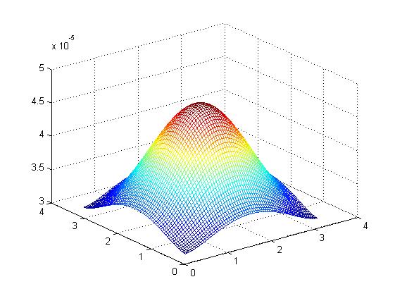
Figure 1: Relative error at $T=0.5$, obtained by algorithm (2.16)$-$(2.17) with mesh $h_{1}=h_{2}=\frac{\pi}{64}$, $\Delta\beta=\frac{1}{64}$, and $\tau=\frac{1}{4096}$.

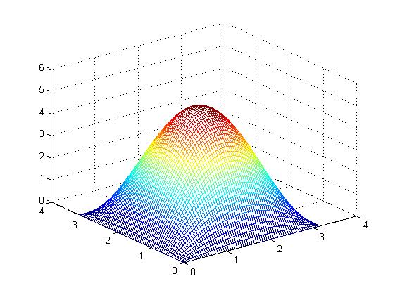
(a)

(b)

Figure 2: Exact solution (a) and approximate solution (b) obtained by algorithm (2.16)$-$(2.17) at $T=0.5$ with mesh $h_{1}=h_{2}=\frac{\pi}{64}$, $\Delta\beta=\frac{1}{64}$, and $\tau=\frac{1}{4096}$.

In Table 1, the numerical accuracy of difference scheme (2.16)$-$(2.17) in time is recorded. Let the step sizes $h_{1}$, $h_{2}$, and $\Delta\beta$ be fixed and small enough such that the dominated error arise from the approximation of the time derivatives. Varying the step sizes in time, the numerical errors in discrete both $L^{\infty}$ and $L^{2}$ norms and the associated convergence orders are shown in this table respectively, which can be found in agreement with the theoretical analysis.

In Table 2, we take the fixed and small enough step sizes in space, and adopt an optimal step size ratio in time and distributed order. As $\Delta\beta$ and $\tau$ vary, we compute the errors and convergence orders listed in the table, which indicates that the convergence order in time and distributed order are about one and two, respectively.

Table 3 displays the computational results with an optimal step size ratio in time, space and distributed order. We can conclude from this table that the convergence orders with respect to time, space and distributed order are approximately one, two and two, respectively, which is in good agreement with our theoretical results analyzed in Section 3.

Table 1: Errors and convergence orders for Example 4.1 in temporal direction with $h_{1}=h_{2}=\frac{\pi}{500}$ and $\Delta\beta=\frac{1}{160}$.

$\tau$	$\big{\|}e^{N}\big{\|}_{L^{\infty}}$	Order	$\big{\|}e^{N}\big{\|}_{L^{2}}$	Order
1/10	0.0839	-	0.1225	-
1/20	0.0439	0.9344	0.0634	0.9502
1/40	0.0227	0.9515	0.0326	0.9596
1/80	0.0117	0.9526	0.0167	0.9650
1/160	0.0059	0.9877	0.0085	0.9743

Table 2: Errors and convergence orders for Example 4.1 with an optimal step size ratio for $\tau$ and $\Delta\beta$, and $h_{1}=h_{2}=\frac{\pi}{500}$.

$\tau$	$\Delta\beta$	$\big{\|}e^{N}\big{\|}_{L^{\infty}}$	Order	$\big{\|}e^{N}\big{\|}_{L^{2}}$	Order
1/100	1/10	0.0093	-	0.0133	-
1/400	1/20	0.0024	1.9542	0.0034	1.9678
1/1600	1/40	6.0481e-04	1.9885	8.6411e-04	1.9762
1/6400	1/80	1.4751e-04	2.0357	2.1076e-04	2.0365

Table 3: Errors and convergence orders for Example 4.1 with an optimal step size ratio for $\tau$, $h_{1}$, $h_{2}$, and $\Delta\beta$.

$\tau$	$h_{1}=h_{2}$	$\Delta\beta$	$\big{\|}e^{N}\big{\|}_{L^{\infty}}$	Order	$\big{\|}e^{N}\big{\|}_{L^{2}}$	Order
1/64	$\pi/2$	1/8	0.4602	-	0.7230	-
1/256	$\pi/4$	1/16	0.1195	1.9453	0.1689	2.0978
1/1024	$\pi/8$	1/32	0.0301	1.9892	0.0426	1.9872
1/4096	$\pi/16$	1/64	0.0075	2.0048	0.0107	1.9932
1/16384	$\pi/32$	1/128	0.0019	1.9809	0.0027	1.9866
1/65536	$\pi/64$	1/256	4.7098e-04	2.0123	6.6801e-04	2.0150

5 Conclusion

In this paper, we construct efficient numerical scheme for solving two-dimensional time-fractional wave equation of distributed-order with a nonlinear source term, and provide the theoretical analysis on stability and convergence by the discrete energy method. Numerical results are provided by figures and tables, which show the algorithm proposed in this work is effective and feasible. In the future work, the promotion of computational efficiency will be considered so that the more complicated problems can be handled.

References

[1]
M. Caputo, Elasticità e dissipazione, Zanichelli, Bologna, 1969.
[2]
Y. G. Sinai, The limiting behavior of a one-dimensional random walk in a random
medium, Theory of Probability & Its Applications 27 (2) (1983) 256–268.
[3]
A. V. Chechkin, J. Klafter, I. M. Sokolov, Fractional Fokker-Planck equation
for ultraslow kinetics, EPL (Europhysics Letters) 63 (3) (2003) 326.
[4]
A. N. Kochubei, Distributed order calculus and equations of ultraslow
diffusion, Journal of Mathematical Analysis and Applications 340 (1) (2008)
252–281.
[5]
C. Eab, S. Lim, Fractional Langevin equations of distributed order, Physical
Review E 83 (3) (2011) 031136.
[6]
Z. Jiao, Y. Chen, I. Podlubny, Distributed-order dynamic systems: stability,
simulation, applications and perspectives. SpringerBriefs in Electrical and
Computer Engineering/SpringerBriefs in Control, Automation and Robotics
(2012).
[7]
M. Caputo, Distributed order differential equations modelling dielectric
induction and diffusion, Fractional Calculus and Applied Analysis 4 (4)
(2001) 421–442.
[8]
T. T. Hartley, C. F. Lorenzo, Fractional system identification: An approach
using continuous order-distributions, 1999.
[9]
A. V. Chechkin, R. Gorenflo, I. M. Sokolov, V. Y. Gonchar, Distributed order
time fractional diffusion equation, Fractional Calculus and Applied Analysis
6 (3) (2003) 259–280.
[10]
T. M. Atanackovic, S. Pilipovic, D. Zorica, Time distributed-order
diffusion-wave equation. I. Volterra-type equation, in: Proceedings of the
Royal Society of London A: Mathematical, Physical and Engineering Sciences,
The Royal Society, 2009, pp. rspa–2008.
[11]
R. Gorenflo, Y. Luchko, M. Stojanović, Fundamental solution of a
distributed order time-fractional diffusion-wave equation as probability
density, Fractional Calculus and Applied Analysis 16 (2) (2013) 297–316.
[12]
Z. Li, Y. Luchko, M. Yamamoto, Asymptotic estimates of solutions to
initial-boundary-value problems for distributed order time-fractional
diffusion equations, Fractional Calculus and Applied Analysis 17 (4) (2014)
1114–1136.
[13]
K. Diethelm, N. J. Ford, Numerical analysis for distributed-order differential
equations, Journal of Computational and Applied Mathematics 225 (1) (2009)
96–104.
[14]
I. Podlubny, T. Skovranek, B. M. V. Jara, I. Petras, V. Verbitsky, Y. Chen,
Matrix approach to discrete fractional calculus III: non-equidistant grids,
variable step length and distributed orders, Phil. Trans. R. Soc. A
371 (1990) (2013) 20120153.
[15]
J. T. Katsikadelis, Numerical solution of distributed order fractional
differential equations, Journal of Computational Physics 259 (2014) 11–22.
[16]
N. J. Ford, M. L. Morgado, M. Rebelo, An implicit finite difference
approximation for the solution of the diffusion equation with distributed
order in time, Electron. Trans. Numer. Anal 44 (2015) 289–305.
[17]
G.-h. Gao, Z.-z. Sun, Two unconditionally stable and convergent difference
schemes with the extrapolation method for the one-dimensional
distributed-order differential equations, Numerical Methods for Partial
Differential Equations 32 (2) (2016) 591–615.
[18]
G.-h. Gao, H.-w. Sun, Z.-z. Sun, Some high-order difference schemes for the
distributed-order differential equations, Journal of Computational Physics
298 (2015) 337–359.
[19]
H. Ye, F. Liu, V. Anh, Compact difference scheme for distributed-order
time-fractional diffusion-wave equation on bounded domains, Journal of
Computational Physics 298 (2015) 652–660.
[20]
G.-h. Gao, Z.-z. Sun, Two alternating direction implicit difference schemes
with the extrapolation method for the two-dimensional distributed-order
differential equations, Computers & Mathematics with Applications 69 (9)
(2015) 926–948.
[21]
G.-h. Gao, Z.-z. Sun, Two alternating direction implicit difference schemes for
two-dimensional distributed-order fractional diffusion equations, Journal of
Scientific Computing 66 (3) (2016) 1281–1312.
[22]
G.-h. Gao, Z.-z. Sun, Two alternating direction implicit difference schemes for
solving the two-dimensional time distributed-order wave equations, Journal of
Scientific Computing 69 (2) (2016) 506–531.
[23]
S. Rida, A. El-Sayed, A. Arafa, On the solutions of time-fractional
reaction–diffusion equations, Communications in Nonlinear Science and
Numerical Simulation 15 (12) (2010) 3847–3854.
[24]
A.-M. Wazwaz, A. Gorguis, An analytic study of fisher’s equation by using
adomian decomposition method, Applied Mathematics and Computation 154 (3)
(2004) 609–620.
[25]
M. L. Morgado, M. Rebelo, Numerical approximation of distributed order
reaction–diffusion equations, Journal of Computational and Applied
Mathematics 275 (2015) 216–227.
[26]
Z. Sun, The method of order reduction and its application to the numerical
solutions of partial differential equations, Science Press, 2009.
[27]
A. Samarskii, V. Andreev, Difference methods for elliptic equations, Nauka,
Moscow, 1976.
[28]
A. Quarteroni, A. Valli, Numerical approximation of partial differential
equations, Vol. 23, Springer Science & Business Media, 2008.