Evolving a Vector Space with any Generating Set

Abstract

In Valiant’s model of evolution, a class of representations is evolvable iff a polynomial-time process of random mutations guided by selection converges with high probability to a representation as $\epsilon$-close as desired from the optimal one, for any required $\epsilon>0$. Several previous positive results exist that can be related to evolving a vector space, but each former result imposes disproportionate representations or restrictions on (re)initialisations, distributions, performance functions and/or the mutator. In this paper, we show that all it takes to evolve a normed vector space is merely a set that generates the space. Furthermore, it takes only $\tilde{O}(1/\epsilon^{2})$ steps and it is essentially stable, agnostic and handles target drifts that rival some proven in fairly restricted settings. Our algorithm can be viewed as a close relative to a popular fifty-years old gradient-free optimization method for which little is still known from the convergence standpoint: Nelder-Mead simplex method.

keywords: Evolvability, vector space, Bregman divergence.

1 Introduction

How can evolution learn ? About a year ago, strong connections between evolution and machine learning at large were highlighted and discussed (Blute, 2016; Jordán, 2016; Livnat and Papadimitriou, 2016; Watson and Szathmáry, 2016a, b; Žliobaitė and Stenseth, 2016). One key open challenge emerged as ”Evo-Devo”, the study of phenotypic variation, the evolution of traits and how these can benefit evolution for future outcomes given that it is essentially a myopic process. This addresses several key observations, (i) the evolutionary process has indeed no anticipation of future outcomes, (ii) the process is randomized and weakly guided by the responses to current conditions. Also, (iii) changes happen at the genotypic level but in fact are observed at a phenotypic level which depends on past selections. Modularity (Hartwell et al., 1999) plays a key role in these: a certain form of intermediate level organisation, modular and multivariate, might facilitate selections through relevant combinations of modules that were successful in the past. Stability is also important as evolution is a still poorly understood balance between change and conservation (Schwenk and Wagner, 2015). We complete Evo-Devo with the capacity of evolution to be (iv) agnostic, (v) adaptive and (vi) distribution-free in the machine learning jargon (Kanade et al., 2010; Valiant, 2009): agnostic because parsimony and model complexity constraints on organisms (Watson and Szathmáry, 2016a) might just prevent selection to reach a perfectly accurate and encodable organism even if carried out forever, adaptive because the ”evolution of evolvability” (Watson and Szathmáry, 2016a) shall require evolution to handle drifts in the optimal organisms (due e.g. to changes in external conditions), and finally distribution-free with respect to conditions to cope with adaptability over long horizon with various environmental conditions (Watson and Szathmáry, 2016a).

The evolvability model of Valiant (2009) is an excellent candidate to frame and formalize such properties, but in the large body of work published on or before Watson and Szathmáry (2016a) in Valiant’s evolvability model, it is quite remarkable that no result frames substantial part of the constraints above, and even less so comes up with a potentially implementable stochastic algorithm. This last question is of practical importance at a time where gradient-free optimization is sparking new interest in computer science and optimization (Nesterov and Spokoiny, 2017).

Our contribution, summarized, is a proof of Valiant’s evolvability for finite-dimensional normed vector spaces using their simplest defining structure, a generating set — and with no distributional assumptions on conditions. In addition, we prove that the same algorithm, which spans few lines of pseudocode, can be made powerful beyond Valiant’s initial requirements, including being agnostic, strictly monotonic, stable and handling significant target drift.

Our proof of evolvability is constructive. In the Evo-Devo scenario, we perform a genotype / phenotype distinction by representing modular components of the phenotypes as functions mapping observable conditions to real-valued vectors (e.g. relative size, height, concentration of certain proteins, etc.). An organism is a linear a combination of these functions, represented by a vector whose coordinates weight each of these. Mutations are represented by a set of vectors in the same space. Incidentally and interestingly, the vocabulary of linear algebra translates to high-level characterizations of the evo-devo regime: for example, pleiotropy may arise from the non-sparsity of a mutation vector (Stearns, 2010), a small number of mutations — in particular not defining a generating set — may indicate parsimony pressure on evolution (Watson and Szathmáry, 2016a), a large number of mutations may indicate genetic redundancy (Kafri et al., 2009) and so on.

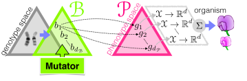
Figure 1: In our model, a phenotype is a linear combination of functions mapping conditions from a set $\mathcal{X}$ to observables in $\mathbb{R}^{d}$ (right). An organism is a linear combination of these, and it is evolved through mutations using a set of vectors $\mathcal{B}$ defining the effect of each mutations on each function of the phenotype (left). The mutator is the Turing-computable mechanism performing mutations in Valiant’s evolvability model (Valiant, 2009) (see text).

The rest of this paper is organised as follows: Section $\S$2 presents related work in Valiant’s evolvability model; $\S$3 details the evolvability model, $\S$4 states and gives a high-level proof of evolvability, $\S$5, $\S$ 6 and $\S$7 respectively state the agnostic, stability and drift-compliant evolvability results and $\S$8 sketches toy experiments. A last $\S$9 discusses and concludes. For space considerations, an Appendix (starting $\S$10) provides all proofs and complete experimental details.

	(A)	(B)	(C)	(D)	(E)	(F)	(G)	(H)	(I)	us
Any target♮	✓	✓	✗	✓	✓	✓	✗	✓	✓	✓
Unrestricted loss†	✗	✗	✗	✗	✓	✗	✗	✗	✗	✓
Weak mutations‡	✗	✓	✓	✗	✗	✗	✓	✗	✗	✓
Non-reflexive neighborhood♡	✗	✗	✗	✗	✗	✗	✗	✗	✗	✓
Optimal sized neighborhood♯	✓	✓	✓	✗	✗	✗	✗	✓	✗	✓
Optimal magnitude (mutations)♭	✓	✓	✓	✗	✗	✗	✗	✓	✗	✓
Strictly monotonic evolution	✓	✓	✓	✗	✗/✓	✓	✓	✓	✓	✓
No distribution assumption	✗	✓	✗	✓	✓	✗	✓	✗	✓	✓
Unknown distribution	✗	✓	✓	✗	✓	✓	✓	✓	✗	✓
Handles agnostic evolution	✗	✓	✗	✗	✗	✗	✗	✗	✗	✓

Table 1: Main related evolvability results (not restricted to vector spaces) and their key properties in the literature (A = Michael (2012), B = Feldman (2009), C = Diochnos and Turán (2009), D = Feldman (2008), E = Valiant (2014), F = Angelino and Kanade (2014), G = Feldman (2011), H = Kanade et al. (2010), I = Feldman (2012)). References indicated in italic can be directly related to evolving vector spaces. ($\natural$) There is no assumption on the target function except its finiteness (encoding). ($\dagger$) “Unrestricted” means that evolution allows twice differentiable non-boolean, non-well-behaved (Feldman, 2011) and non-quadratic losses. ($\ddagger$) Weak mutations: modifications do not depend on the current organism. ($\heartsuit$) Non-reflexive: neighborhood does not contain the current organism. ($\sharp$) Neighborhood size always $O({d_{\mbox{\tiny{${\mathcal{P}}$}}}})$. ($\flat$) Mutations magnitude is $\Omega(\epsilon)$. The gray column relates to the simplest form of organisms addressed, singletons (Feldman, 2009).

2 Related work and comparison

In Leslie Valiant’s model (Valiant, 2009), evolution has to come with high probability $\epsilon$-close to the optimum after a polynomial number of iterations. Evolution makes local modifications to a function that acts as an organism and weakly minimizes a loss function through a mutator (shown in Figure 1). There has been a large amount of work in the evolvability model, summarized in Table 1 (the Table is discussed in Section $\S$ 9). Row “non-reflexive neighborhood” is a new feature that we have found nowhere else: the fact that the current organism $f$ does not belong to the mutant set forces the mutator to evolve $f$ without the safety net that reflexive mutations belong to neutral neighbors, which therefore somewhat artificially contain “worst case” evolution. Perhaps the work that is the closest to ours with respect to the framework is that of Paul Valiant (Valiant, 2014), which evolves organisms encoding reals instead of binary number as in Valiant (2009) — a setting arguably closer to natural biological processes. In Valiant (2014), the problem corresponds to the restriction of Figure 1 for $\mathcal{X}=\mathbb{R}^{n}$ and phenotypes being fixed-degree polynomials. There are two key contributions in the work of Valiant (2014). The first one, which we relate to as the ”indirect approach”, works under a broad setting which parallels ours : any convex loss and any distribution on $\mathcal{X}$. We call it indirect because it relies on the beautiful recording trick that representations can ”hardcode” the optimisation steps of evolution (Feldman, 2008, 2009; Valiant, 2014). This trick comes however with some significant downsides. First, the coding size of representations grows at each generation and ultimately depend on the desired accuracy for evolution. In particular, it is polynomial in $1/\epsilon$, which can be huge. Second, the mutator simulates a weak optimiser and so the time complexity for each mutation is also big, more precisely of the order of the time complexity of the weak optimisation algorithm it emulates times the coding size of the maximal performance. Third and worse, evolution comes with restart: at each generation, there is a chance that all past evolution history is wiped out and the representation is initialized to a default one.

The second contribution of Valiant (2014) is more direct since it trades the complex mutator for a much simpler and randomized hill climber. However, the analysis is now significantly more restricted as evolution is proven only for the quadratic loss and the distribution is restricted to a ball on $\mathcal{X}$. Also, evolution still suffers downsides as the coding size expands at each generation and the mutator is computationally quite ineffective and biologically unplausible: the neighborhood to find new mutants size is huge — polynomial in $1/\epsilon$ and other factors — and it resamples its stock of available mutations at each generation. Finally, neither of Valiant (2014)’s schemes are known to be agnostic nor stable in any way — we note that stability is an important notion in biology (Schwenk and Wagner, 2015) but is not a feature of Valiant’s original evolvability model.

Our main result suffers none of these downsides: our mutator meets time and space optimality properties (Section 9), we do not change the set of mutations (Section 4), we do not do restart. Also, our evolvability scheme is agnostic (Section 5), stable (Section 6) and handles significant drift (Section 7). Finally, instead of fixed-degree polynomials, we consider any finite-valued function $f:\mathcal{X}\rightarrow\mathbb{R}^{d}$. Thus, we can evolve functions with infinite Taylor expansion, something Valiant (2014) does not cover. Finally, our mutator yields an extremely simple and provable evolutionary scheme, implementable using few lines of code as sketched in Algorithm 1 ($\mathsf{Simple\mbox{-}Evol\mbox{-}Gen}$).

As a brief comparison with other work, the mutator is not organism-dependent like in (Kanade et al., 2010), we have no distribution assumptions like in (Angelino and Kanade, 2014; Kanade et al., 2010) or a requirement to know this distribution like in (Feldman, 2008), and the same scheme can be made agnostic or handle drift more significant than some allowed in more restricted settings (Kanade et al., 2010). We insists on the no-distribution assumption: in some work, this distribution is constrained, smooth and nice (Angelino and Kanade, 2014), uniform (Michael, 2012; Valiant, 2009), spherically symmetric (Kanade et al., 2010), a product of Gaussians with polynomial variance (Kanade et al., 2010), or with support restricted to a ball (Valiant, 2014).

Algorithm 1 $\mathsf{Simple\mbox{-}Evol\mbox{-}Gen}$($f_{0}$)

  Input: initial representation $f_{0},T$;

  For $t=0,1,...,T-1$

   Step $t$.1: Sample $\mathcal{S}$ as per (5);

   Step $t$.2: Compute $\textsc{Bene}(f_{t})$ and $\textsc{Neut}(f_{t})$ using $\textsc{n}_{\epsilon}(f_{t})$ as per (4)

   Step $t$.3: if $\textsc{Bene}(f_{t})\neq\emptyset$ then sample uniformly $f_{t+1}$ in $\textsc{Bene}(f_{t})$ as per (1);

       else if $\textsc{Neut}(f_{t})\neq\emptyset$ then sample uniformly $f_{t+1}$ in $\textsc{Neut}(f_{t})$ as per (2);

       else sample uniformly $f_{t+1}$ in $\textsc{n}_{\epsilon}(f_{t})$;

  Return $f_{T}$;

3 Evolvability model

We define key components of the Evolvability model and then define the model (Valiant, 2009).

Topology of representations —

Organisms are represented by functions $f:{\mathcal{X}}\rightarrow{\mathbb{R}}^{d}$ of a set ${{\mathcal{P}}}$ (Figure 1), called the representation class, supposed to be polynomial-time Turing-evaluatable. ${\mathcal{X}}$ is the set of conditions or experiences. For any $f\in{{\mathcal{P}}}$, a neighborhood function is defined, $\textsc{n}_{\epsilon}(f)\subseteq{{\mathcal{P}}}$, that depends on an accuracy parameter $\epsilon>0$. The size of the neighborhood is required to be polynomial in $1/\epsilon$, $d$ and the dimension of ${\mathcal{X}}$, $\mathrm{dim}({\mathcal{X}})$.

Performances of representations —

Performances are measured with respect to an unknown but fixed distribution ${\mathcal{D}}$ over ${\mathcal{X}}$, relatively to an unknown target function $t\in{{\mathcal{P}}}$. The expected performance of some $f\in{{\mathcal{P}}}$ with respect to $t$ is $\texttt{Perf}_{t,\varphi}(f,{\mathcal{D}})\stackrel{{\scriptstyle\mathrm{.}}}{{=}}-\mathbb{E}_{x\sim{\mathcal{D}}}[D_{\varphi}(f(x)\|t(x))]$, where $D_{\varphi}$ is Bregman divergence with (twice differentiable) generator $\varphi:{\mathbb{R}}^{d}\rightarrow{\mathbb{R}}$ (Bregman, 1967; Banerjee et al., 2005a, b; Boissonnat et al., 2010). By extension, the empirical performance realized by $f$ on an i.i.d. sample ${\mathcal{S}}$ is defined as $\texttt{Perf}_{t,\varphi}(f,{\mathcal{S}})\stackrel{{\scriptstyle\mathrm{.}}}{{=}}-\mathbb{E}_{x\sim{\mathcal{S}}}[D_{\varphi}(f(x)\|t(x))]$. Our expected performance $\texttt{Perf}_{t,\varphi}$ generalizes Valiant’s which computes $\mathbb{E}_{{\mathcal{D}}}[ft]$. In Valiant’s setting, $d=1$, the output of functions is $\{-1,1\}$ and $D_{\varphi}$ is the square loss $D_{\footnotesize{\textsc{sql}}}$, and so $\texttt{Perf}_{t,\footnotesize{\textsc{sql}}}(f,{\mathcal{D}})=2(\mathbb{E}_{{\mathcal{D}}}[f(x)t(x)]-1)$. Notice that unlike Valiant (2014), we do not assume to know the functions defining phenotypes in Figure 1 (grey parallelogram), we just observe the combination of their outputs. We consider it very natural, some sort of “Petri dish” model of performance evaluation.

Selection by mutations —

A mutator $\textsc{Mut}:{{\mathcal{P}}}\times{\mathbb{N}}\rightarrow{{\mathcal{P}}}\cup\{\bot\}$ is a randomized polynomial-time Turing machine that depends upon an accuracy $\epsilon>0$ and a tolerance $\textsc{T}>0$. Tolerance is required to be polynomial in $\epsilon$, $1/d$ and $1/\mathrm{dim}({\mathcal{X}})$. The mutator returns a so-called “mutant” of some input $f\in{{\mathcal{P}}}$ based on a weak evaluation of the quality of the elements of $\textsc{n}_{\epsilon}(f)$. More precisely, it takes as input a sample size $m>0$, samples i.i.d. a set ${\mathcal{S}}$ of $m$ conditions, and outputs some $g\in\textsc{Bene}(f)$ at random if $\textsc{Bene}(f)\neq\emptyset$, or else $g\in\textsc{Neut}(f)$ at random if $\textsc{Neut}(f)\neq\emptyset$, using a fixed distribution $\upmu(g,f)$ with support $\textsc{Bene}(f)$ or $\textsc{Neut}(f)$. Those two sets $\textsc{Bene}(f)$ and $\textsc{Neut}(f)$ are defined respectively by:

$$\textsc{Bene}(f) \stackrel{{\scriptstyle\mathrm{.}}}{{=}} \{g\in\textsc{n}_{\epsilon}(f):\texttt{Perf}_{t,\varphi}(g,{\mathcal{S}})\geq\texttt{Perf}_{t,\varphi}(f,{\mathcal{S}})+\textsc{T}\}\>\>,$$ (1)

$$\textsc{Neut}(f) \stackrel{{\scriptstyle\mathrm{.}}}{{=}} \{g\in\textsc{n}_{\epsilon}(f):|\texttt{Perf}_{t,\varphi}(g,{\mathcal{S}})-\texttt{Perf}_{t,\varphi}(f,{\mathcal{S}})|<\textsc{T}\}\>\>.$$ (2)

If both sets $\textsc{Bene}(f)$ and $\textsc{Neut}(f)$ are empty, the mutator outputs $\bot$, meaning evolution has failed.

Representations —

Our framework being non-boolean, we define the models that we evolve. Let $[n]\stackrel{{\scriptstyle\mathrm{.}}}{{=}}\{0,1,...,n\}$ and $[n]_{*}\stackrel{{\scriptstyle\mathrm{.}}}{{=}}\{1,...,n\}$ where $n$ is a natural integer. First, we have a set of functions $\{g_{1},g_{2},...,g_{{d_{\mbox{\tiny{${\mathcal{P}}$}}}}}\}\subset{{\mathcal{P}}}$, each of which is of the form $g_{j}:{\mathcal{X}}\rightarrow{\mathbb{R}}^{d}$ for $j\in[{d_{\mbox{\tiny{${\mathcal{P}}$}}}}]$ for some ${d_{\mbox{\tiny{${\mathcal{P}}$}}}}>0$. Each $g_{j}$ can be thought as encoding a specific part of trait(s) representation, such as a relative concentration in specific proteins under any experimental condition — for this reason we suppose without loss of generality that its norm $\|g_{j}(.)\|_{2}^{2}$ is finite almost everywhere with respect to $\mathcal{D}$. The set of functions that we evolve lies in the span of $\{g_{1},g_{2},...,g_{{d_{\mbox{\tiny{${\mathcal{P}}$}}}}}\}$ — which we also denote as ${\mathcal{P}}$ for simplicity —, i.e., consists of linear combinations of functions of ${\mathcal{P}}$. However, because we want our model to be general, we do not evolve directly ${\mathcal{P}}$. For this reason, we define a set of vectors ${\mathcal{B}}\stackrel{{\scriptstyle\mathrm{.}}}{{=}}\{b_{1},b_{2},...,b_{{d_{\mbox{\tiny{$\mathcal{B}$}}}}}\}$, with $b_{i}\in\mathbb{R}^{{d_{\mbox{\tiny{${\mathcal{P}}$}}}}}$, that will represent our set of mutations. Each (column) vector, $b_{i}\stackrel{{\scriptstyle\mathrm{.}}}{{=}}[b_{i}^{1}\cdots b_{i}^{{d_{\mbox{\tiny{${\mathcal{P}}$}}}}}]^{\top}$ maps to a function $b_{i}(x)\stackrel{{\scriptstyle\mathrm{.}}}{{=}}\sum_{j}b_{i}^{j}\cdot g_{j}(x)$. Their span, $\mathrm{span}(\mathcal{B})$, defines a subspace of the phenotype vector space. While we will investigate first the case $\mathrm{span}(\mathcal{B})={\mathcal{P}}$, we shall also cover the ”agnostic” evolvability case where $\mathrm{span}(\mathcal{B})\subset{\mathcal{P}}$. An organism $f$ that our mutator builds has evolved from some initial $f_{0}$ and can therefore be represented as $f=f_{0}+\sum_{i}f^{i}b_{i}$, where $[f^{1}\>f^{2}\>...\>f^{{d_{\mbox{\tiny{$\mathcal{B}$}}}}}]\in{\mathbb{N}}^{{d_{\mbox{\tiny{$\mathcal{B}$}}}}}$. Finally, To avoid confusion with ${\mathbb{R}}^{d}$, we let $\|.\|_{{\mathcal{P}}}$ denote the $L_{2}$ norm computed with respect to $\{g_{1},g_{2},...,g_{{d_{\mbox{\tiny{${\mathcal{P}}$}}}}}\}$, i.e. the norms of the coordinates in ${\mathcal{P}}$.

Evolvability horizon —

In the same way as PAC-learnability allows to be polynomial in the size of the target concept, evolvability has to allow a time complexity that depends on some complexity measure with respect to the target organism, and not just the number of description variables, which would be $\mathrm{dim}({\mathcal{X}})$ in our case. Evolvability results involving complex representations alleviate this distinction by putting constraints on representations (Kanade et al., 2010; Valiant, 2014). We integrate this notion in the form of what we call the Evolvability horizon, $T_{\textsc{d}}$. $T_{\textsc{d}}$ quantifies the necessary number of generations to come up with an encoding “close” to that of $t$. Any evolution using $o(T_{\textsc{d}})$ generations, using only $\mathcal{B}$, would be bound to fail in the worst case.

Definition 3.1

The Evolvability horizon $T_{\textsc{d}}(f_{0},t)$ ($T_{\textsc{d}}$ for short) of $f_{0}$ wrt target $t$ is $T_{\textsc{d}}\stackrel{{\scriptstyle\mathrm{.}}}{{=}}\left\lceil\frac{\|t-f_{0}\|_{{\mathcal{P}}}}{\max_{i}\|b_{i}\|_{{\mathcal{P}}}}\right\rceil$.

Evolvability —

We define evolvability, following (Feldman, 2009; Valiant, 2009).

Definition 3.2

Assume the following fixed, for any accuracy $\epsilon>0$: representation class ${{\mathcal{P}}}$, mutator neighborhood $\textsc{n}_{\epsilon}$ and distribution $\mu$, distribution ${\mathcal{D}}$, generator $\varphi$, tolerance T. Then ${{\mathcal{P}}}$ is distribution-free evolvable by mutator $\textsc{Mut}(.,.)$ iff for any initial representation $f_{0}$ and target representation $t$ such that $T_{\textsc{d}}\ll\infty$ (”$\ll\infty$” means finite), there exist polynomial functions $m$ and $T$ (both polynomial in $d,\mathrm{dim}({\mathcal{X}}),1/\epsilon,T_{\textsc{d}}$) such that $\forall 0<\epsilon\leq 1$, then with probability $\geq 1-\epsilon$, the sequence $f_{0},f_{1},...,f_{T}$ with $f_{j}\stackrel{{\scriptstyle\mathrm{.}}}{{=}}\textsc{Mut}(f_{j-1},m)$, $\forall j$, satisfies:

$$\texttt{Perf}_{t,\varphi}(f_{T},{\mathcal{D}}) \geq -\epsilon\>\>.$$ (3)

Our model of evolution holds without initialisation (Feldman, 2008; Valiant, 2009). We have simplified the presentation of the model, in particular removing the notion of “evolution algorithm” and specifying evolution directly from the mutator. This does not weaken the results.

4 Evolvability of vector spaces

The main notations are summarized in Appendix, Subsection 11.1.

Definition 4.1

A mutator is permissible iff the neighborhood used by the mutator is defined as:

$$\textsc{n}_{\epsilon}(f) \stackrel{{\scriptstyle\mathrm{.}}}{{=}} \{f\}\oplus\{\sigma\alpha b_{i}:\sigma\in\{-1,+1\},b_{i}\in{\mathcal{B}}\}\>\>,$$ (4)

for some set ${\mathcal{B}}\stackrel{{\scriptstyle\mathrm{.}}}{{=}}\{b_{1},b_{2},...,b_{{d_{\mbox{\tiny{$\mathcal{B}$}}}}}\}$, where $\oplus$ is Minkowski sum. $\alpha>0$ (fixed) is called the magnitude of the mutations and $\sigma$ is called the polarity of the mutation.

We have not detailed the distribution of the mutator, $\upmu$ (Section 3). In fact, it can be any distribution with full support and (at least) inversely polynomial density, following e.g., (Kanade et al., 2010). We shall consider the simplest of all, the uniform distribution. We remark that ${\mathcal{B}}$ is not necessarily a basis, nor normal, nor orthogonal. Also, $\alpha$ is the key parameter to be tuned for evolvability. We evolve vector spaces under three assumptions united in a Singularity-Free (SF) setting.

Definition 4.2

The (SF) setting is defined by the following three assumptions:
(i) any genome “can be coded”: $\mathrm{span}(\mathcal{B})={{\mathcal{P}}}$,
(ii) any target organism $t$ is “unique”: $\arg\min_{f}\texttt{Perf}_{t,\varphi}(f,{\mathcal{D}})=\{t\}$ ($\forall t\in{\mathcal{P}}$), and
(iii) any non-void genome gets “expressed”: $\mathbb{P}_{x\sim\mathcal{D}}[g(x)\neq 0_{{\mathbb{R}}^{d}}]>0,\forall g\neq 0_{\mathcal{P}}$.

Each of (i-iii) allows to define parameters that will be useful to quantify evolution. We now provide a concise version of our main results, hiding the less important parameters in the corresponding $\theta,\tilde{O}$ notations (the complete statement of the Theorem is in Theorem 11.1).

Theorem 4.1

(evolvability of vector spaces, concise statement) Assume (SF) holds. Then ${{\mathcal{P}}}$ is distribution-free evolvable by any permissible mutator Mut, with tolerance $\textsc{T}=\theta(\epsilon^{2})$ and magnitude of mutations $\alpha=\theta(\epsilon)$. The number of conditions sampled at each iteration satisfies:

$$m = \tilde{O}\left(\frac{T_{\textsc{d}}^{4}}{\epsilon^{2}}\log\left(\frac{{d_{\mbox{\tiny{$\mathcal{B}$}}}}T_{\textsc{d}}}{\epsilon}\right)\right)\>\>.$$ (5)

Finally, the number of evolution steps $T$ sufficient to comply with ineq. (3) is $T=\tilde{O}\left(T_{\textsc{d}}^{4}/\epsilon^{2}\right)$.

We sketch the key steps for the proof of Theorem 4.1, first introducing key definitions 4.3 and 4.4 below.

Definition 4.3

For any representation $f$, condition $x$, magnitude $\alpha$ and polarity $\sigma$, we let

$$\mathrm{R}_{f,i}(x) \stackrel{{\scriptstyle\mathrm{.}}}{{=}} \langle\sigma b_{i}(x),(\nabla\varphi\circ t)(x)-(\nabla\varphi\circ f)(x)\rangle\>\>,\mbox{ and }$$ (6)

$$\Pi_{f,i}(x) \stackrel{{\scriptstyle\mathrm{.}}}{{=}} \frac{1}{\alpha}D_{\varphi}(f(x)-\alpha\cdot(-\sigma)b_{i}(x)\|f(x))$$ (7)

denote respectively the mutator’s return and premium on $x$ given $f$, omitting $\sigma$ and $\alpha$ in notations.

We give an equivalent definition for the set of beneficial mutations, using returns and premiums.

Lemma 4.1

$\textsc{Bene}(f)=\left\{f+\sigma\alpha b_{i}\in\textsc{n}_{\epsilon}(f):\mathbb{E}_{{\mathcal{S}}}[\mathrm{R}_{f,i}(x)]-\mathbb{E}_{{\mathcal{S}}}[\Pi_{f,i}(x)]\geq(\textsc{T}/\alpha)\right\}$.

(Proof in Appendix, Subsection 11.3) We call Lemma 4.1 the mean-divergence decomposition of beneficial mutations in reference to portfolio theory: when $D_{\varphi}$ is Mahalanobis divergence, the model simplifies to an equivalent of Markowitz model (Markowitz, 1952) in which $\Pi_{f,i}(x)=(\alpha/2)\cdot\langle b_{i}(x),\mbox{{\normalsize{m}}}b_{i}(x)\rangle$ (m symmetric positive definite), i.e. the magnitude of mutations $\alpha$ is exactly Arrow-Pratt measure of absolute risk aversion — since $\alpha>0$, evolution is ”risk averse”. Due to the lack of space, we close this analogy here and notice that the mutator’s premium quantifies the (local) risk of mutating (it does not depend on $t$). Hereafter, we let “expected” return and “expected” premium denote the expectation of (6) and (7). There is a quantity that turns out to be key in our analysis. It ties expression (phenotype) and encoding (genotype), the pg-ratio.

Definition 4.4

The phenotype-to-genotype (pg) ratio of $f\in{{\mathcal{P}}}$ given distribution ${\mathcal{D}}$ is:

$$\rho(f|{{\mathcal{D}}}) \stackrel{{\scriptstyle\mathrm{.}}}{{=}} \frac{\mathbb{E}_{{\mathcal{D}}}[\|f(x)\|^{2}_{2}]}{\|f\|_{{{\mathcal{P}}}}}=\frac{\mathrm{Var}_{{\mathcal{D}}}[\|f(x)\|_{2}]+(\mathbb{E}_{{\mathcal{D}}}[\|f(x)\|_{2}])^{2}}{\|f\|_{{{\mathcal{P}}}}}\>\>.$$ (8)

The pg-divergence between $f\in{{\mathcal{P}}}$ and $g\in{{\mathcal{P}}}$ given distribution ${\mathcal{D}}$ is $\rho(f,g|{{{\mathcal{D}}}})\stackrel{{\scriptstyle\mathrm{.}}}{{=}}\rho(f-g|{{\mathcal{D}}})$.

A justification for the name of $\rho(f,g|{{{\mathcal{D}}}})$ comes from the fact that $\rho(f|{{\mathcal{D}}})=\rho(f,0_{{{\mathcal{P}}}}|{{{\mathcal{D}}}})$, $0_{{{\mathcal{P}}}}$ representing a “void genome”. The proof of Theorem 4.1 relies on two arguments. The first establishes that, provided the mutator samples sufficient conditions $m$, the set of beneficial mutations is never empty with high probability, as long as the current $f$ is “far” from the optimum, where this distance notion relies on the pg-divergence between $f$ and the target $t$. In fact, we show a bit more, as in this case mutations may be superior beneficial: we call them superior beneficial because while beneficial mutations shall be proven to yield an improvement of $\Omega(\epsilon^{2})$ in performance, those superior beneficial mutations yield a greater increase of $\Omega(\epsilon)$. In the second argument, we show that when the first argument does not hold anymore, the requirements of evolvability are met, and the number of evolution steps is polynomial in all required parameters, so vector spaces are evolvable. To formalize these two arguments, we need to define an important basis in $\mathcal{B}$, called $\mathcal{B}^{*}$.

Definition 4.5

Let $\mathcal{B}^{*}\subseteq\mathcal{B}$ be a basis that maximises $\overline{B}_{{\mathcal{P}}}(\mathcal{B}^{\prime})\stackrel{{\scriptstyle\mathrm{.}}}{{=}}B_{{\mathcal{P}}}(\mathcal{B}^{\prime})/\max_{b\in\mathcal{B}^{\prime}}\|b\|_{\mathcal{P}}$ over all bases $\mathcal{B}^{\prime}\subseteq\mathcal{B}$, where $B_{{\mathcal{P}}}(\mathcal{B}^{\prime})\stackrel{{\scriptstyle\mathrm{.}}}{{=}}(1-\kappa_{n}(\mathcal{B}^{\prime}))\cdot(1-\kappa_{a}(\mathcal{B}^{\prime}))\cdot\frac{\sum_{b\in\mathcal{B}^{\prime}}\|b\|_{{\mathcal{P}}}}{{d_{\mbox{\tiny{${\mathcal{P}}$}}}}}$ and $\kappa_{n}(\mathcal{B}^{\prime})$ and $\kappa_{a}(\mathcal{B}^{\prime})$ denote non-negative reals such that $G(\mathcal{B}^{\prime})=(1-\kappa_{n}(\mathcal{B}^{\prime})^{\frac{2}{{d_{\mbox{\tiny{${\mathcal{P}}$}}}}}}A(\mathcal{B}^{\prime})$, $\cos(\theta_{\mbox{\tiny{${\mathcal{V}}$}}})=1-(1-\kappa_{a}(\mathcal{B}^{\prime}))^{\frac{1}{{d_{\mbox{\tiny{${\mathcal{P}}$}}}}-1}}$. Here, $G(.)$ and $A(.)$ are the geometric and arithmetic means of the squared norms in $\mathcal{B}^{\prime}$, and $\theta_{\mbox{\tiny{${\mathcal{V}}$}}}\stackrel{{\scriptstyle\mathrm{.}}}{{=}}\min_{b\neq b^{\prime}\in\mathcal{B}^{\prime}}\min\{|\angle b,b^{\prime}|,|\pi-\angle b,b^{\prime}|\}\in[0,\pi/2]$ is the minimal angle between two vectors.

Roughly, the larger $B_{{\mathcal{P}}}(.)$, the better for evolution. This parameter tends to be larger as the basis in argument becomes closer to orthonormality, and so orthonormal bases represent the “easiest” cases for evolution from this standpoint. They turn out to be the ones of (Kanade et al., 2010, Section 6).

Lemma 4.2

$\forall{\mathcal{B}}^{\prime}$ a basis of ${\mathcal{P}}$, $B_{{\mathcal{P}}}(\mathcal{B}^{\prime})$ and $\overline{B}_{{\mathcal{P}}}(\mathcal{B}^{\prime})$ are strictly positive.

Proof: If $\kappa_{n}({\mathcal{B}}^{\prime})=1$, then one vector in ${\mathcal{B}}^{\prime}$ is the null vector, if $\kappa_{a}({\mathcal{B}}^{\prime})=1$, then two vectors in ${\mathcal{B}}^{\prime}$ are collinear, in whichever case ${\mathcal{B}}^{\prime}$ cannot be a basis. Thus, $(\kappa_{n}({\mathcal{B}}^{\prime}),\kappa_{a}({\mathcal{B}}^{\prime}))\in[0,1)^{2}$. Finally, no basis vector can be the null vector, so $B_{{\mathcal{P}}}(\mathcal{B}^{\prime})>0$ and $\overline{B}_{{\mathcal{P}}}(\mathcal{B}^{\prime})>0$, as claimed.        Wlog, we are assume $\max_{i\in[{d_{\mbox{\tiny{$\mathcal{B}$}}}}]_{*}}\|b_{i}\|_{{\mathcal{P}}}=\max_{b_{i}\in\mathcal{B}^{*}}\|b_{i}\|_{{\mathcal{P}}}$, and $\sup_{i,x}\omega(\mathcal{B}^{\prime}\cup\{b_{i}\},x)\leq\sup_{x}\omega(\mathcal{B}^{*},x)$ for any basis $\mathcal{B}^{\prime}\subseteq\mathcal{B}$ and $b_{i}\in\mathcal{B}$, where $\omega(\mathcal{B}^{\prime},x)\stackrel{{\scriptstyle\mathrm{.}}}{{=}}\sum_{b_{i}\in\mathcal{B}^{\prime}}\|b_{i}(x)\|^{2}_{2}$ for any $\mathcal{B}^{\prime}\subseteq\mathcal{B}$ and any $x\in{\mathcal{X}}$. These assumptions simplify derivations without restricting our results. We also assume $\sup_{x}\omega(\mathcal{B}^{*},x)$ polynomial in all genome parameters, $d,\mathrm{dim}(\mathcal{X})),T_{\textsc{d}}$, in order not to laden the polynomial dependences of the evolvability model by one which takes into account the maximal magnitude of expressions. We denote $\Psi\stackrel{{\scriptstyle\mathrm{.}}}{{=}}\mathbb{E}_{x\sim{\mathcal{D}}}[\mbox{{\normalsize{g}}}^{\top}_{x}\mbox{{\normalsize{g}}}_{x}]$ where $\mbox{{\normalsize{g}}}^{\top}_{x}$ stacks all $g_{i}(x)$ in column, and $0\leq\gamma\leq\gamma^{\prime}\ll\infty$ (resp. $0\leq\mu\leq\mu^{\prime}\ll\infty$) the min/max eigenvalues of the Hessian of $\varphi$ (resp. $\Psi$).

Lemma 4.3

Under (SF), $\gamma>0$ and $\mu>0$.

Indeed, if $\gamma=0$, then (ii) in (SF) would be violated. If $\mu=0$, some genomes would get expressed only on conditions sets of zero measure, violating (iii) in (SF). We define four sets of organisms. The first, ${{\mathcal{P}}}_{t}$, is the set complying with evolvability requirements as in ineq. (3). The second, ${{\mathcal{P}}}_{t,{\mathcal{D}}}$, is the set of organisms ”far enough” from target relatively to the pg-divergence.

Definition 4.6

Let ${{\mathcal{P}}}_{t}\stackrel{{\scriptstyle\mathrm{.}}}{{=}}\{f\in{{\mathcal{P}}}:\texttt{Perf}_{t,\varphi}(f,{\mathcal{D}})\geq-\epsilon\}$, and

$${{\mathcal{P}}}_{t,{\mathcal{D}}} \stackrel{{\scriptstyle\mathrm{.}}}{{=}} \left\{f\in{{\mathcal{P}}}:\exists b_{i}\in\mathcal{B}^{*},\rho(f,t|{{{\mathcal{D}}}})\geq\frac{\sqrt{e{d_{\mbox{\tiny{${\mathcal{P}}$}}}}}}{\gamma B_{{\mathcal{P}}}({\mathcal{B}}^{*})}\left(\tau+\alpha{\gamma^{\prime}}\cdot\|b_{i}\|_{{\mathcal{P}}}\cdot\rho(b_{i}|{{{\mathcal{D}}}})+\frac{\textsc{T}}{\alpha}\right)\right\}\>\>,$$ (9)

where $\alpha,\tau,\textsc{T}>0$ are fixed beforehand. Let ${{\mathcal{P}}}_{t,{\mathcal{D}}}\supseteq{\mathcal{P}}_{\mbox{\tiny{{mon}}}}\stackrel{{\scriptstyle\mathrm{.}}}{{=}}\{f_{j}:f_{j^{\prime}}\in{{\mathcal{P}}}_{t,{\mathcal{D}}},\forall j^{\prime}\in[j]\}$, where $f_{j}\stackrel{{\scriptstyle\mathrm{.}}}{{=}}\textsc{Mut}(f_{j-1},m)$, and $\overline{{\mathcal{P}}}_{\mbox{\tiny{{mon}}}}\stackrel{{\scriptstyle\mathrm{.}}}{{=}}\{f_{j}\}_{j=1}^{T}\backslash{\mathcal{P}}_{\mbox{\tiny{{mon}}}}$ the sequence “following” ${\mathcal{P}}_{\mbox{\tiny{{mon}}}}$.

Hence, ${\mathcal{P}}_{\mbox{\tiny{{mon}}}}$ is the longest prefix sequence of evolved organisms that are all in ${{\mathcal{P}}}_{t,{\mathcal{D}}}$. Note that we do not assume that ${\mathcal{P}}_{\mbox{\tiny{{mon}}}}\neq\emptyset$. A key property of ${\mathcal{P}}_{\mbox{\tiny{{mon}}}}$ is that its sequence of organisms has strictly monotonically increasing performances and yields with high probability non-empty beneficial sets. This is our first argument to the proof of Theorem 4.1.

Theorem 4.2

Assume (SF) holds. Suppose $\alpha,\tau,\textsc{T}>0$ fixed, and mutator is run for $T>0$ iterations, sampling at each iteration a number of conditions

$$m = \Omega\left(\frac{{\gamma^{\prime}}^{2}\sup_{x}\omega^{2}(\mathcal{B}^{*},x)}{\tau^{2}}\left(\frac{\gamma^{\prime}\mu^{\prime}}{\gamma\mu}\cdot\frac{T_{\textsc{d}}^{2}}{\overline{B}^{2}_{{\mathcal{P}}}(\mathcal{B}^{*})}+\alpha^{2}\right)\log\left(\frac{{d_{\mbox{\tiny{$\mathcal{B}$}}}}T}{\epsilon}\right)\right)\>\>.$$ (10)

Then, recalling that $f_{j}\stackrel{{\scriptstyle\mathrm{.}}}{{=}}\textsc{Mut}(f_{j-1},m)$, the following holds true with probability $\geq 1-\epsilon$:

$$\textsc{Bene}(f_{j}) \neq \emptyset\>\>,\forall f_{j}\in{\mathcal{P}}_{\mbox{\tiny{{mon}}}}\>\>.$$ (11)

Lemma 4.4

If $\overline{{\mathcal{P}}}_{\mbox{\tiny{{mon}}}}\neq\emptyset$, then let $\overline{{\mathcal{P}}}_{\mbox{\tiny{{mon}}}}\stackrel{{\scriptstyle\mathrm{.}}}{{=}}\{f_{j}\}_{j=j_{\star}}^{T}$ for some $j_{\star}\in[T]^{*}$. Then $f_{j_{\star}}\in{{\mathcal{P}}}_{t}$.

(Proofs respectively in Appendix, Subsection 11.4 and Subsection 11.5) Hence, the first element in $\overline{{\mathcal{P}}}_{\mbox{\tiny{{mon}}}}$ complies with evolvability requirements in eq. (3). What remains to be shown is that as long as the current organism $f_{j}$ stays in ${\mathcal{P}}_{\mbox{\tiny{{mon}}}}$ ($\subseteq{{\mathcal{P}}}_{t,{\mathcal{D}}}$), the performance increases by a substantial amount, guaranteeing that the following scenario occurs: either at some point it escapes ${\mathcal{P}}_{\mbox{\tiny{{mon}}}}$, in which case Lemma 4.4 guarantees that evolvability requirements are met, or it never escapes ${{\mathcal{P}}}_{t,{\mathcal{D}}}$ and after a polynomial number of iterations, it satisfies evolvability requirements as well, achieving our second argument. This is shown in the following Lemma.

Lemma 4.5

Fix T and $\alpha$ as in (23) and (24), and in eqs (9, 10) let $\tau\stackrel{{\scriptstyle\mathrm{.}}}{{=}}\theta(\epsilon/U)$, with $U\stackrel{{\scriptstyle\mathrm{.}}}{{=}}(\gamma^{\prime\frac{3}{2}}\mu^{\prime\frac{1}{2}}/(\gamma^{\frac{3}{2}}\mu^{\frac{1}{2}}))\cdot(2\sqrt{e{d_{\mbox{\tiny{${\mathcal{P}}$}}}}}/\overline{B}_{{\mathcal{P}}}({\mathcal{B}}^{*}))\cdot T_{\textsc{d}}$. Then, with probability $\geq 1-\epsilon$, $(f_{j}\in{\mathcal{P}}_{\mbox{\tiny{{mon}}}})\Rightarrow\texttt{Perf}_{t,\varphi}(f_{j+1},{\mathcal{D}})=\texttt{Perf}_{t,\varphi}(f_{j},{\mathcal{D}})+\Omega(\epsilon^{2}),\forall j\in[T]_{*}$. Finally, the number of evolution steps sufficient for ${\mathcal{P}}_{\mbox{\tiny{{mon}}}}$ to comply with (3) is $T=\tilde{O}\left(T_{\textsc{d}}^{4}/\epsilon^{2}\right)$.

(Proof in Appendix, Subsection 11.6) This completes the proof sketch of Theorem 4.1. Section 11 in the Appendix (pages 11-15) provides the complete proof.

5 Agnostic evolvability of vector spaces

One important question is what happens when $t$ cannot be evolved from $\mathcal{B}$, i.e. when alleviating condition (i) in setting (SF). Ideally, we would like evolution to converge to the “best” evolvable organism in terms of performances. To our knowledge, few positive result exist in the agnostic / improper evolvability model (Angelino and Kanade, 2014; Feldman, 2009), and the most unrestricted one holds for extremely simple representations: singletons (Feldman, 2009). Neither evolving schemes of Valiant (2014) are known to be agnostic. The proof of the following Theorem appears in Appendix, Section 12.

Theorem 5.1

If we relax assumption (i) in (SF) but keep (ii, iii), then Theorem 4.1 holds mutatis mutandis with the replacement of ineq. (3) by:

$$\texttt{Perf}_{t,\varphi}(f_{T},{\mathcal{D}}) \geq \sup_{f\in\mathrm{span}(\mathcal{B})}\texttt{Perf}_{t,\varphi}(f,{\mathcal{D}})-\epsilon\>\>.$$ (12)

6 Beyond Valiant’s evolvability: stable evolvability of vector spaces

The evolution of phenotypes is an important but still poorly understood phenomenon, mixing both the tendency to adapt to changing environments and the ”need” to remain the same (Schwenk and Wagner, 2015). In Valiant’s evolvability model, one would expect the later constraint to prevail when the organism is close enough to the optimum — a good mutator should not jump from a near-optimal organism to a highly suboptimal one, except perhaps with sufficiently small probability. Valiant model does not take this into account: all that is required is to probably ”hit” the $\epsilon$-closedness ”ball” around the optimum in polynomial time (ineq. (3)) and with high probability. Nothing is required for what happens ”next”. This is not a desirable feature since it does not preclude one of the poorest mutators — a coin — to be efficient: if there are two organisms in a set $\mathcal{Z}$, say $A$ (optimal) and $b$ (highly suboptimal), then any coin ”mutator” with fixed bias (even favouring the choice of $b$) trivially ”evolves” $\mathcal{Z}$ : $O(\log(1/\epsilon))$ mutations suffice to hit $A$ with high probability. If we were to require evolution to ”stay” $\epsilon$-close to the optimum for a certain number of iterations when it satisfies the conditions of evolvability, this would considerably impede such poorly informed mutators. To our knowledge, there is no such stability result in Valiant’s model. We now provide such a result.

Theorem 6.1

Assume (SF) holds. Let $N\in\mathbb{N}_{*}$. Then Theorem 4.1 holds mutatis mutandis with the replacement of ineq. (3) by: $\texttt{Perf}_{t,\varphi}(f_{T+j},{\mathcal{D}})\geq-\epsilon$, $\forall j\in[N]$.

(Proof in Appendix, Section 14) Note that stability can be controlled by tuning $N$.

7 Evolvability of vector spaces with target drift

Another important question is what happens when the target organism drifts slowly (Kanade et al., 2010). In (Kanade et al., 2010), there is a sequence of targets $t_{0},t_{1},...$ and the objective is to replace the static requirement in ineq. (3) by one which takes into account the last target $t_{T}$, when $t_{i}$ is allowed to slightly drift with respect to $t_{i-1}$ with respect to its performances. In our case, since we separate the encoding from computing performances, we allow the encoding to drift, which is perhaps more natural — drift affects genotype before performances. Also, the evaluation of beneficial and neutral mutations in Bene and Neut are done for $f_{j-1}$ with respect to $t_{j-1}$.

Theorem 7.1

Assume (SF) holds and the target organism sequence $t_{0},t_{1},...$ drifts according to $\|t_{i+1}-t_{i}\|_{\mathcal{P}}\leq\tilde{O}\left(\epsilon^{4}/(T_{\textsc{d}}^{2}\max_{i^{\prime}\in[{d_{\mbox{\tiny{$\mathcal{B}$}}}}]_{*}}\|b_{i^{\prime}}\|^{2}_{{\mathcal{P}}})\right)$, $\forall i\geq 0$. Then Theorem 4.1 holds mutatis mutandis with the replacement of ineq. (3) by: $\texttt{Perf}_{t_{T},\varphi}(f_{T},{\mathcal{D}})\geq-\epsilon$.

(Proof in Appendix, Section 13) Up to factors that depend upon $\gamma,\gamma^{\prime},\mu,\mu^{\prime}$, our model of drift is equivalent to the performance drift model of (Kanade et al., 2010) (see Lemma 11.8 below), yet, as a function of $\epsilon$, we tolerate drifts that are larger by factor $\theta(1/\epsilon^{2})$ than theirs, taking as reference their result on the weakest distribution assumptions (product Gaussians), assumptions that we also alleviate. Dependence on $T_{\textsc{d}}$ is necessary up to some extent, as otherwise worst-case drifts would defeat evolution by artificially increasing the actual horizon to the last target ($T_{\textsc{d}}$ is computed for $t_{0}$). It is important to note that (Kanade et al., 2010, Theorem 8, Corollary 9) show that the strict monotonicity of evolution — that is, the fact that performance satisfies some minimal strictly positive increment from one generation on to the next — is sufficient to grant some resistance against drift. From this standpoint, the indirect approach (Section 2 above) of Valiant (2014) is not a good candidate since it does restart. The direct approach however, which operates with the square loss and on a ball-supported distribution, displays strict monotonicity, yet a direct application of (Kanade et al., 2010, Theorem 8) shows drift resistance with poor dependence on the degree of the evolved polynomial, i.e. of order $1/(\dim(\mathcal{X}))^{\mbox{\tiny{degree}}}$ in the worst case (Valiant, 2014, Proof of Theorem 3.3).

8 Toy experiments

Table 2: Toy supervised learning experiment. Left: performances, indicating the $-\epsilon$ evolvability threshold in green. The data (shown on the right: black / grey = positive / negative class) are not linearly separable, so we compute the performance minus that of the optimal linear separator (eq. (12)). Organisms evolved are also displayed on the right (the cyan / dark blue path = path followed by the arrowhead of the vector learned, starting from the null vector). Dark blue means that the organism satisfies the condition of the evolvability model (eq. (12)). A red vector displays the target, almost confounded with the last vector evolved (dark blue line, best viewed in color).

We complete our results with preliminary toy experiments in supervised and unsupervised learning, displaying some promising directions for Evolvability to spin out provable stochastic gradient-free optimization algorithms, a field that has recently started to spark new interest (Nesterov and Spokoiny, 2017). The algorithm we use is a slightly more specific version of Algorithm 1 above, presented in Appendix (Section 16). We sketch here the supervised experiments and refer to Appendix, Section 16 for a complete presentation of all experiments. Our supervised problem is the approximation of the best linear classifier on non-separable data. Table 2 presents the results obtained on a dataset also displayed. While it has no pretention whatsoever to bring significant experimental support for the theory developed, it displays interesting patterns of convergence: the conditions for evolvability to be met are achieved quite early in the process, and the the presence of failures in the supervised case does not prevent evolution to reach classifiers close to the optimal classifier.

9 Discussion and conclusion

We split the discussion in several parts.

Bregman divergences — We chose Bregman divergence for several reasons. First, they generalize performance functions previously used in seminal approaches (Kanade et al., 2010; Valiant, 2009) and they are in no way restrictive: the minimisation of any differentiable convex function attaining its global minimum is trivially equivalent to the minimisation of a Bregman divergence. Moreover, they exhaustively define fundamental classes of loss functions of both supervised and unsupervised learning (Banerjee et al., 2005b; Nock and Nielsen, 2008; Reid and Williamson, 2010) and their properties are well understood: we use them to analyze our mean-divergence model from Lemma 4.1 and devise a generalized Pythagoras’ Theorem trick for agnostic evolvability in Theorem 5.1.

Grid-convex minimization on a non-complete space — Evolvability can be analyzed from the standpoint of the actual space in which evolution takes place from the mutator (not every representation may be built). For example, in the case of Valiant (2014), the direct approach needs a complete vector space because the mutator samples in a topological closed ball. This is not our case: any permissible mutator (Definition 4.1) evolves organisms on a grid — finer as $\epsilon$ decreases, but always a grid — so in theory, we do not need a complete vector space. For that reason, we do not need a performance convex everywhere: it just needs to be convex on this grid. Our result is not the first to enjoy such a property: a quick inspection shows that it is also the case for (Kanade et al., 2010, Section 6.1). Our analysis is however significantly more general and would allow the efficient minimization of highly non-convex functions whose minima define a convex function supported on a grid, a notorious example of which being Griewank function (Griewank, 1981).

Optimality of the mutator, frugality of evolution — Evolution is fundamentally a resource-constrained process (Pekkonen et al., 2013), so it makes a lot of sense to analyze evolvability in the light of time and space requirements, in particular for the key algorithmic device of evolution, the mutator. It is not hard to check that our mutator is optimal essentially up to factor 2: suppose $\mathcal{B}$ defines a basis for ${\mathcal{P}}$. Any mutator running under the constraint to be able to generate the whole space needs to work in time and space $\Omega(\mathrm{Card}(\mathcal{B}))$, a lowerbound indeed matched by ours. We also note the frugality of our evolution process, since our mutator never changes the set of mutations. All these properties are enjoyed by (Kanade et al., 2010, Section 6.1); none of them is enjoyed by the approaches of Valiant (2014). However, mention of the possibility to use of the canonical basis to improve the mutator is given (footnote 2 in Valiant (2014)), yet without proof but noting the difficulty of the task. We note that we are significantly more general than this possibility, since we consider not just orthonormal bases, but any generating set.

Random gradient-free optimization — Derivative-free optimization is a big field intersecting mathematics, computer science and engineering (Conn et al., 2008), comprising a variety of methods like genetic algorithms. Our approach to evolvability certainly bears similarities with that class of algorithms, but it is eventually closer to another popular set, Nelder-Mead simplex methods (Nelder and Mead, 1965; Nesterov and Spokoiny, 2017). Briefly, such methods transform a deformable non-degenerate simplex using a set of (initially five) possible moves, including reflection, expansion, etc. . When our generating set is a basis, we can represent our algorithm with a rigid simplex modified by a set of two operations only: ”mirroring” the simplex to account for the polarity of mutations, and ”translating” it to follow mutations. While our setting is not comparable to the deterministic setting of Nesterov and Spokoiny (2017), we obtain dependences in $\epsilon$ similar to theirs on non-strongly convex optimisation, without using the directional secant information that they use.

Evolution on the efficient frontier — Our brief analogy with Markowitz’ portfolio theory (Markowitz, 1952) following Lemma 4.1 can be carried out much further to analytically compute the efficient frontier of evolution. This appears to be an important question because such a frontier has been documented in systems biology (Kitano, 2010); interestingly, when the current organism is “far” from the target (in a specific sense), all superior beneficial mutations are close to the efficient frontier, and therefore display an approximately optimal risk-return tradeoff. This observation, formalized and proven in the Appendix (Section 15), sheds interesting new light to the systems biology’s observations (Kitano, 2010) that go beyond the scope of our paper.

To summarize, what we have shown is that, to evolve a vector space, one merely needs a norm and a set that generates the space. The resulting algorithm essentially has a single free parameter ($\alpha$, Definition 4.1) and is straightforward to implement. Our result generalizes in several directions another close result (Feldman, 2011) (Theorems 4.1, 4.4), i.e., outside the binary classification framework, the realm of well-behaved losses, single-dimensional outputs and non-agnostic evolvability. Our framework is also more general. Feldman requires the target organism to have minimal non-zero margin over all conditions, which is equivalent to replacing the non-zero probability by a unit probability in assumption (iii) of setting (SF), and therefore weakens the general purpose of the result — even when the minimal margin assumption is reasonable in the restricted binary classification setting. Finally, our analysis displays better dependences on the key parameters $\alpha,T,m$: inspection of the bounds of Feldman shows that the guarantees on performance increase may be very loose, namely as small as $\tilde{O}(\epsilon^{a})$ for some potentially large constant $a$, which is significantly worse than our $\tilde{\Omega}(\epsilon^{2})$ guarantee in ${\mathcal{P}}_{\mbox{\tiny{{mon}}}}$.

Appendix — Table of contents

Overview of our results Pg 10
Proof of Theorem 4.1 Pg 11
Proof of Theorem 5.1 Pg 12
Proof of Theorem 6.1 Pg 14
Evolution on the efficient frontier Pg 15
Toy experiments (full) Pg 16

10 Overview of our results

Figure 2 presents a complete synthetic view of the main mechanisms shown in our paper (including in the Appendix), with two properties never explicitly documented before: the fact that the apparent weakness of the mutator (which works regardless of the set that generates ${{\mathcal{P}}}$) does not prevent it to be able to “compete” with the best mutators when far from the target, and the fact that evolution may just be trapped “close” to the target when it has succeeded. The agnostic evolution setting relies on an analogue to Bregman orthogonal projection theorems (Amari and Nagaoka, 2000) involving the performance function.

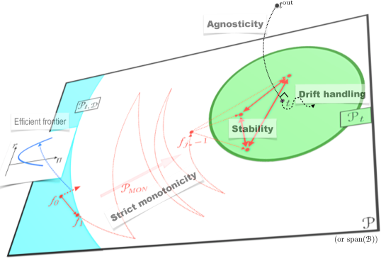
Figure 2: Summary of our results — Evolvability as carried out by our simple mutator (in red), with high probability: sequence ${\mathcal{P}}_{\mbox{\tiny{{mon}}}}$ monotonically converges to an organism that satisfies the conditions of evolvability (green area), after which monotonicity may not hold anymore, but many subsequent organisms may satisfy the conditions of evolvability. When far from the target (blue), our mutator always has access to mutations close to the efficient frontier of evolution (diagram). If $t$ is not evolvable ($t^{\mathrm{out}}$), then evolution converges to the “closest” encodable target. Stability also guarantees that when the evolved organism satisfies the conditions of evolvability, it will do so for at least a certain number of following generations. All notions developed in the main body of the paper are indicated in bold faces. The notion of efficient frontier is developed in the Appendix only (best viewed in color).

11 Proof of Theorem 4.1

11.1 Basic notations and helper Lemmata

$t$	target organism
$f_{j}$	evolved organism
${\mathcal{B}}^{\prime}$	basis $\subseteq\mathcal{B}$
$\mbox{{\normalsize{b}}}^{\prime}$	${d_{\mbox{\tiny{${\mathcal{P}}$}}}}\times{d_{\mbox{\tiny{${\mathcal{P}}$}}}}$ transition matrix for basis ${\mathcal{B}}^{\prime}$ in orthonormal “gene” basis $\{g_{1},g_{2},..,g_{d_{\mbox{\tiny{${\mathcal{P}}$}}}}\}$
$\delta(x)$	$\stackrel{{\scriptstyle\mathrm{.}}}{{=}}(t-f)(x)=\mbox{{\normalsize{g}}}_{x}\mbox{{\normalsize{b}}}^{*}(t-f)$,
	difference of expressions between target $t$ and organism $f$
	measured with respect to basis ${\mathcal{B}}^{*}$
$\delta^{i}$	coordinate $i$ of vector $\delta$
$\|.\|_{\mathcal{P}}$	norm in canonical (“gene”) basis of ${\mathcal{P}}$
$g_{i}$	canonical basis vector of ${\mathcal{P}}$
$g_{i}(x)$	gene expression output (in ${\mathbb{R}}^{d}$) of $g_{j}$ on some $x\in{\mathcal{X}}$
$\mbox{{\normalsize{g}}}_{x}$	$\stackrel{{\scriptstyle\mathrm{.}}}{{=}}[g_{1}(x)|g_{2}(x)|\cdots|g_{{d_{\mbox{\tiny{${\mathcal{P}}$}}}}}(x)]\in{\mathbb{R}}^{d\times{d_{\mbox{\tiny{${\mathcal{P}}$}}}}}$
	per-gene output matrix on some $x\in{\mathcal{X}}$
$\Psi$	$\stackrel{{\scriptstyle\mathrm{.}}}{{=}}\mathbb{E}_{x\sim{\mathcal{D}}}[\mbox{{\normalsize{g}}}^{\top}_{x}\mbox{{\normalsize{g}}}_{x}]\in{\mathbb{R}}^{{d_{\mbox{\tiny{${\mathcal{P}}$}}}}\times{d_{\mbox{\tiny{${\mathcal{P}}$}}}}}$
$\mathrm{ker}(.)$	null space

Unless otherwise stated, all organisms are expressed in basis $\mathcal{B}^{*}\subseteq\mathcal{B}$, that is,

$$f(x) = \mbox{{\normalsize{g}}}_{x}\mbox{{\normalsize{b}}}^{*}f\>\>,$$ (13)

and the norm of the encoding of $f$ expressed in basis $\mathcal{B}^{*}$ shall be

$$\|f\|_{{\mathcal{P}}} \stackrel{{\scriptstyle\mathrm{.}}}{{=}} \sqrt{\langle\mbox{{\normalsize{b}}}^{*}f,\mbox{{\normalsize{b}}}^{*}f\rangle}\>\>.$$ (14)

We use in several places the following Lemmata.

Lemma 11.1

Under setting (SF), there exists symmetric positive definite matrix m such that $\mathbb{E}_{{\mathcal{D}}}[\mathrm{R}_{f,i}(x)]=\langle\mbox{{\normalsize{b}}}^{*}b_{i},\mbox{{\normalsize{m}}}\mbox{{\normalsize{b}}}^{*}\delta\rangle,\forall b_{i}\in{\mathcal{B}}$ (coordinates of $\delta\stackrel{{\scriptstyle\mathrm{.}}}{{=}}t-f,b_{i}$ expressed in basis ${\mathcal{B}}^{*}$).

Proof: Because $\varphi$ is twice differentiable and strictly convex, a Taylor expansion of $\nabla\varphi$ around $t(x)$ yields

$$(\nabla\varphi\circ t)(x) = (\nabla\varphi\circ f)(x)+\textsc{h}(x)(t-f)(x)$$ (15)

$$= (\nabla\varphi\circ f)(x)+\textsc{h}(x)\mbox{{\normalsize{g}}}_{x}\mbox{{\normalsize{b}}}^{*}\delta\>\>,$$

for some value of the Hessian $\textsc{h}(x)$ of $\varphi$, therefore symmetric positive definite. We get

$$\mathbb{E}_{{\mathcal{D}}}[\langle b_{i}(x),(\nabla\varphi\circ t)(x)-(\nabla\varphi\circ f)(x)\rangle] = \mathbb{E}_{{\mathcal{D}}}[\langle\mbox{{\normalsize{g}}}_{x}\mbox{{\normalsize{b}}}^{*}b_{i},\textsc{h}(x)\mbox{{\normalsize{g}}}_{x}\mbox{{\normalsize{b}}}^{*}\delta\rangle]$$

$$= \mathbb{E}_{{\mathcal{D}}}[\langle\mbox{{\normalsize{b}}}^{*}b_{i},\mbox{{\normalsize{g}}}^{\top}_{x}\textsc{h}(x)\mbox{{\normalsize{g}}}_{x}\mbox{{\normalsize{b}}}^{*}\delta\rangle]$$

$$= \langle\mbox{{\normalsize{b}}}^{*}b_{i},\mathbb{E}_{{\mathcal{D}}}[\mbox{{\normalsize{g}}}^{\top}_{x}\textsc{h}(x)\mbox{{\normalsize{g}}}_{x}]\mbox{{\normalsize{b}}}^{*}\delta\rangle$$

$$\stackrel{{\scriptstyle\mathrm{.}}}{{=}} \langle\mbox{{\normalsize{b}}}^{*}b_{i},\mbox{{\normalsize{m}}}\mbox{{\normalsize{b}}}^{*}\delta\rangle\>\>,$$

with

m $$\stackrel{{\scriptstyle\mathrm{.}}}{{=}} \mathbb{E}_{{\mathcal{D}}}[\mbox{{\normalsize{g}}}^{\top}_{x}\textsc{h}(x)\mbox{{\normalsize{g}}}_{x}]\>\>.$$ (16)

Because of (iii) in (SF), for any $g\neq 0_{\mathcal{P}}\in{\mathcal{P}}$, for each $x\in\mathcal{X}$ for which it is expressed, we have $g(x)=\mbox{{\normalsize{g}}}_{x}\mbox{{\normalsize{b}}}^{*}g\neq 0_{{\mathbb{R}}^{d}}$ and so

$$\langle\mbox{{\normalsize{b}}}^{*}g,\mbox{{\normalsize{m}}}\mbox{{\normalsize{b}}}^{*}g\rangle = \int_{\mathcal{X}}p(x)\langle g(x),\textsc{h}(x)g(x)\rangle\mathrm{d}x$$

$$\geq \mathbb{P}_{x\sim\mathcal{D}}[g(x)\neq 0_{{\mathbb{R}}^{d}}]\cdot\min_{g(x)\neq 0_{{\mathbb{R}}^{d}}}\langle g(x),\textsc{h}(x)g(x)\rangle$$

$$> 0\>\>,$$

showing m is positive definite.       

Lemma 11.2

Under setting (SF), for any $f,t\in{\mathcal{P}}$ (coordinates expressed in basis $\mathcal{B}^{*}$), the following holds, for some $\mbox{{\normalsize{m}}}^{\prime}$ symmetric positive definite:

$$\mathbb{E}_{x\sim{\mathcal{D}}}[D_{\varphi}(f(x)\|t(x))] = \langle\mbox{{\normalsize{b}}}^{*}(f-t),\mbox{{\normalsize{m}}}^{\prime}\mbox{{\normalsize{b}}}^{*}(f-t)\rangle\>\>,$$ (17)

$$\mathbb{E}_{x\sim{\mathcal{D}}}[D_{\varphi}(f(x)\|t(x))] \in \left[\frac{\gamma}{2}\cdot\langle\mbox{{\normalsize{b}}}^{*}(f-t),\Psi\mbox{{\normalsize{b}}}^{*}(f-t)\rangle,\frac{\gamma^{\prime}}{2}\cdot\langle\mbox{{\normalsize{b}}}^{*}(f-t),\Psi\mbox{{\normalsize{b}}}^{*}(f-t)\rangle\right]\>\>.$$ (18)

Proof: Both results are a consequence of (Amari and Nagaoka, 2000), that for any twice differentiable $\varphi$,

$$D_{\varphi}(f(x)\|t(x)) = \frac{1}{2}\cdot\langle\mbox{{\normalsize{g}}}_{x}\mbox{{\normalsize{b}}}^{*}(f-t),\mbox{{\normalsize{h}}}(x)\mbox{{\normalsize{g}}}_{x}\mbox{{\normalsize{b}}}^{*}(f-t)\rangle\>\>,$$ (19)

for some value of the Hessian $\mbox{{\normalsize{h}}}(x)$ of $\varphi$, therefore symmetric positive definite. Then, we define $\mbox{{\normalsize{m}}}^{\prime}$ as

$$\mbox{{\normalsize{m}}}^{\prime} \stackrel{{\scriptstyle\mathrm{.}}}{{=}} \frac{1}{2}\cdot\mbox{{\normalsize{m}}}\>\>,$$ (20)

where m is defined in eq. (16), and so $\mbox{{\normalsize{m}}}^{\prime}\succ 0$. We then use the definition of $\gamma$ to obtain ineq. (18).       

11.2 Complete statement of Theorem 4.1

We first provide a more complete statement of Theorem 4.1. We now define two key parameters:

$$U \stackrel{{\scriptstyle\mathrm{.}}}{{=}} \frac{\gamma^{\prime\frac{3}{2}}\mu^{\prime\frac{1}{2}}}{\gamma^{\frac{3}{2}}\mu^{\frac{1}{2}}}\cdot\frac{2\sqrt{e{d_{\mbox{\tiny{${\mathcal{P}}$}}}}}}{\overline{B}_{{\mathcal{P}}}({\mathcal{B}}^{*})}\cdot T_{\textsc{d}}\>\>,$$ (21)

$$V \stackrel{{\scriptstyle\mathrm{.}}}{{=}} {\gamma^{\prime}}\cdot\max_{i\in[{d_{\mbox{\tiny{$\mathcal{B}$}}}}]_{*}}\{\mathbb{E}_{{\mathcal{D}}}[\|b_{i}(x)\|^{2}_{2}]\}\>\>,$$ (22)

and triples of evolution “knobs”, $(z_{\tau},z_{\alpha},z_{\textsc{T}})\in{\mathbb{R}}_{+*}^{3}$, all absolute constants.

Definition 11.1

Set $\mathfrak{R}\subset{\mathbb{R}}^{3}$ is defined as the subset of triples $(z_{1},z_{2},z_{3})$ such that (i) $z_{1},z_{2},z_{3}>0$, (ii) $z_{3}-z_{1}z_{2}>0$, (iii) $z_{2}^{2}-z_{2}(1-z_{1})+z_{3}\leq 0$.

Remark that $\mathfrak{R}\neq\emptyset$, since for example $(1/9,1/3,2/27)\in\mathfrak{R}$. We now state our main result.

Theorem 11.1

(evolvability of vector spaces, complete statement) Assume (SF) holds, and fix any $(z_{\tau},z_{\alpha},z_{\textsc{T}})\in\mathfrak{R}$. ${{\mathcal{P}}}$ is distribution-free evolvable by any permissible mutator Mut, with tolerance:

T $$\stackrel{{\scriptstyle\mathrm{.}}}{{=}} \frac{z_{\textsc{T}}}{U^{2}\max\{1,V\}}\cdot\epsilon^{2}=\theta(\epsilon^{2})\>\>,$$ (23)

and magnitude of mutations:

$$\alpha \stackrel{{\scriptstyle\mathrm{.}}}{{=}} \frac{z_{\alpha}}{U\max\{1,V\}}\cdot\epsilon=\theta(\epsilon)\>\>.$$ (24)

The number of conditions sampled at each iteration satisfies:

$$m = O\left(\frac{\gamma^{\prime 6}\mu^{\prime 2}\sup_{x}\omega^{2}(\mathcal{B}^{*},x)}{\gamma^{4}\mu^{2}}\cdot\frac{1}{\overline{B}^{4}_{{\mathcal{P}}}(\mathcal{B}^{*})}\cdot\frac{T_{\textsc{d}}^{4}}{\epsilon^{2}}\log\left(\frac{{d_{\mbox{\tiny{$\mathcal{B}$}}}}T_{\textsc{d}}}{\epsilon}\right)\right)=\tilde{O}\left(\frac{T_{\textsc{d}}^{4}}{\epsilon^{2}}\log\left(\frac{{d_{\mbox{\tiny{$\mathcal{B}$}}}}T_{\textsc{d}}}{\epsilon}\right)\right)\>\>.$$ (25)

Finally, the number of evolution steps $T$ sufficient to comply with ineq. (3) is $T=\tilde{O}\left(T_{\textsc{d}}^{4}/\epsilon^{2}\right)$.

Remark that $z_{\tau}$ is defined but not used in the Theorem statement. It shall be used in its proof below.

11.3 Proof of Lemma 4.1

By definition,

$$\textsc{Bene}(f) = \{g\in\textsc{n}_{\epsilon}(f):\texttt{Perf}_{t,\varphi}(g,{\mathcal{S}})\geq\texttt{Perf}_{t,\varphi}(f,{\mathcal{S}})+\textsc{T}\}$$ (28)

$$= \{g\in\textsc{n}_{\epsilon}(f):\mathbb{E}_{{\mathcal{S}}}[\langle g(x)-f(x),(\nabla\varphi\circ t)(x)-(\nabla\varphi\circ f)(x)\rangle-D_{\varphi}(g(x)\|f(x))]\geq\textsc{T}\}$$

$$= \left\{\begin{array}[]{l}f+\sigma\alpha b_{i}\in\textsc{n}_{\epsilon}(f):\mathbb{E}_{{\mathcal{S}}}\left[\langle\sigma b_{i}(x),(\nabla\varphi\circ t)(x)-(\nabla\varphi\circ f)(x)\rangle\right]\\ -\mathbb{E}_{{\mathcal{S}}}\left[\frac{1}{\alpha}D_{\varphi}((f+\alpha\cdot\sigma b_{i})(x)\|f(x))\right]\geq\frac{\textsc{T}}{\alpha}\end{array}\right\}$$

$$= \left\{f+\sigma\alpha b_{i}\in\textsc{n}_{\epsilon}(f):\mathbb{E}_{{\mathcal{S}}}[\mathrm{R}_{f,i}(x)]-\mathbb{E}_{{\mathcal{S}}}[\Pi_{f,i}(x)]\geq\frac{\textsc{T}}{\alpha}\right\}\>\>,$$ (29)

as claimed (end of the proof of Lemma 4.1).

11.4 Proof of Theorem 4.2

The proof of the Theorem consists of the following building blocks:

• we show a result more general than eq. (11), namely, over all steps $j\in[T]_{*}$ and with high probability:

  $$\left(\exists b_{i}\in\mathcal{B}^{*}:\rho(f_{j},t|{{{\mathcal{D}}}})\geq\frac{\sqrt{e{d_{\mbox{\tiny{${\mathcal{P}}$}}}}}}{\gamma B_{{\mathcal{P}}}(\mathcal{B}^{*})}\left(\tau+\alpha{\gamma^{\prime}}\cdot\|b_{i}\|_{{\mathcal{P}}}\cdot\rho(b_{i}|{{{\mathcal{D}}}})+\frac{\textsc{T}}{\alpha}\right)\right)$$ (30)

  $$\Rightarrow\textsc{Bene}(f_{j})\neq\emptyset\>\>.$$

  This is more general since we show that eq. (11) holds for all organisms of the evolution sequence that belong to ${{\mathcal{P}}}_{t,{\mathcal{D}}}$, and not just the “first” ones in ${\mathcal{P}}_{\mbox{\tiny{{mon}}}}$. To have this with high probability it is sufficient to sample $m=\tilde{\Omega}(\max_{j}\|t-f_{j}\|_{{\mathcal{P}}}^{2})$ conditions, which may be hard to upperbound depending on $f_{j}$;

• we show that, in the subsequence ${\mathcal{P}}_{\mbox{\tiny{{mon}}}}$, $\max_{j}\|t-f_{j}\|_{{\mathcal{P}}}^{2}$ may be conveniently upperbounded.

$\hookrightarrow$ (Proof of [BB.1]) We temporarily drop subscript $j$ in $f_{j}$ for clarity. The proof involves the following three steps. First, we show that for any current representation $f$, there always exist a mutation whose expected return is at least a (positive) fraction of the pg-divergence between $f$ and the target $t$. Its proof involves a simple lowerbound on the volume induced by an arbitrary basis of vectors, which may be of independent interest. Second, we show that, in the evolvability setting, this mutation is special: whenever the current representation $f$ is in ${\mathcal{P}}_{\mbox{\tiny{{mon}}}}$, there is always $\sigma\in\{-1,1\},b_{i}\in{\mathcal{B}}$ such that

$$\mathbb{E}_{{\mathcal{D}}}[\mathrm{R}_{f,i}(x)]-\mathbb{E}_{{\mathcal{D}}}[\Pi_{f,i}(x)] \geq \frac{\textsc{T}}{\alpha}+\tau\>\>.$$ (31)

We shall see that this guarantees equivalently $\mathbb{E}_{{\mathcal{D}}}[\mathrm{R}_{f,i}(x)]-\mathbb{E}_{{\mathcal{D}}}[\Pi_{f,i}(x)]=\Omega(\epsilon)$ — we call this mutation superior beneficial, since the right hand side exceeds the beneficial requirements (eq. (29)) by $\tau$, and furthermore the left hand side is measured on ${\mathcal{D}}$. Third and last, even when the mutation picked is not superior beneficial, sampling a number of examples large enough is sufficient to guarantee $\textsc{Bene}(f)\neq\emptyset$. More precisely, when $m$ is large enough, the sum of the two differences between $(\mathbb{E}_{{\mathcal{D}}}[\mathrm{R}_{f,i}(x)]-\mathbb{E}_{{\mathcal{D}}}[\Pi_{f,i}(x)])$ and $(\mathbb{E}_{{\mathcal{S}}}[\mathrm{R}_{f,i}(x)]-\mathbb{E}_{{\mathcal{S}}}[\Pi_{f,i}(x)])$ in absolute value is at most $\tau$ over each of the $T$ iterations, with probability $\geq 1-\epsilon$. Using (31) then proves the statement of the Theorem because of the definition of $\textsc{Bene}(f)$ in (29).

Lemma 11.3

Assume (SF) holds. Then for any distribution ${\mathcal{D}}$ and any representations $t,f\in{{\mathcal{P}}}$ with coordinates expressed in basis $\mathcal{B}^{*}$,

$$\max_{b_{i}\in\mathcal{B}^{*}}{|\mathbb{E}_{{\mathcal{D}}}[\mathrm{R}_{f,i}(x)]|} \geq K\cdot\rho(f,t|{{{\mathcal{D}}}})\>\>,$$ (32)

where

$$K \stackrel{{\scriptstyle\mathrm{.}}}{{=}} \frac{\gamma}{\sqrt{e{d_{\mbox{\tiny{${\mathcal{P}}$}}}}}}\cdot B_{{{\mathcal{P}}}}(\mathcal{B}^{*})\>\>,$$ (33)

and $B_{{{\mathcal{P}}}}(\mathcal{B}^{*})$ is the corrected average norm in Definition 4.5.

Proof: The majority of the proof consists in showing first that ineq. (32) holds for

$$K \stackrel{{\scriptstyle\mathrm{.}}}{{=}} \frac{\gamma}{\sqrt{e}}\cdot\left(\frac{G(\mathcal{B}^{*})^{{d_{\mbox{\tiny{${\mathcal{P}}$}}}}}}{A(\mathcal{B}^{*})^{{d_{\mbox{\tiny{${\mathcal{P}}$}}}}-1}}\cdot\frac{(1-\cos(\theta_{\mbox{\tiny{${\mathcal{B}}^{\prime}$}}}))^{{d_{\mbox{\tiny{${\mathcal{P}}$}}}}-1}\cdot(1+({d_{\mbox{\tiny{${\mathcal{P}}$}}}}-1)\cdot\cos(\theta_{\mbox{\tiny{${\mathcal{B}}^{\prime}$}}}))}{{d_{\mbox{\tiny{${\mathcal{P}}$}}}}}\right)^{\frac{1}{2}}\>\>,$$ (34)

where parameters $G(\mathcal{B}^{*}),A(\mathcal{B}^{*}),\theta_{\mbox{\tiny{${\mathcal{B}}^{\prime}$}}}$ are defined in Definition 4.5. Then, we show that ineq. (32) holds for the expression of $K$ in eq. (33). Define for short:

$$\delta \stackrel{{\scriptstyle\mathrm{.}}}{{=}} t-f=\sum_{i\in{d_{\mbox{\tiny{${\mathcal{P}}$}}}}}\delta^{i}b_{i}\>\>,$$ (35)

assuming without loss of generality that $\mathcal{B}^{*}\stackrel{{\scriptstyle\mathrm{.}}}{{=}}\{b_{1},b_{2},...,b_{{d_{\mbox{\tiny{${\mathcal{P}}$}}}}}\}$. From Lemma 11.1, there exists symmetric positive definite matrix m such that $\mathbb{E}_{{\mathcal{D}}}[\mathrm{R}_{f,i}(x)]=\langle b_{i},\mbox{{\normalsize{m}}}\mbox{{\normalsize{b}}}^{*}\delta\rangle,\forall b_{i}\in{\mathcal{B}}^{*}$. This allows to get the last equality of:

$$\langle\mbox{{\normalsize{b}}}^{*}\delta,\mbox{{\normalsize{m}}}\mbox{{\normalsize{b}}}^{*}\delta\rangle = \sum_{i\in[{d_{\mbox{\tiny{${\mathcal{P}}$}}}}]}\delta^{i}\cdot\langle b_{i},\mbox{{\normalsize{m}}}\mbox{{\normalsize{b}}}^{*}\delta\rangle$$ (37)

$$\leq \left(\sum_{i\in[{d_{\mbox{\tiny{${\mathcal{P}}$}}}}]}{(\delta^{i})^{2}}\right)^{\frac{1}{2}}\left(\sum_{i\in[{d_{\mbox{\tiny{${\mathcal{P}}$}}}}]}{\langle b_{i},\mbox{{\normalsize{m}}}\mbox{{\normalsize{b}}}^{*}\delta\rangle}\right)^{\frac{1}{2}}$$

$$\leq \sqrt{{d_{\mbox{\tiny{${\mathcal{P}}$}}}}}\max_{i\in[{d_{\mbox{\tiny{${\mathcal{P}}$}}}}]}{|\langle b_{i},\mbox{{\normalsize{m}}}\mbox{{\normalsize{b}}}^{*}\delta\rangle|}\cdot\left(\sum_{i\in[{d_{\mbox{\tiny{${\mathcal{P}}$}}}}]}{(\delta^{i})^{2}}\right)^{\frac{1}{2}}$$

$$=\sqrt{{d_{\mbox{\tiny{${\mathcal{P}}$}}}}}\max_{i\in[{d_{\mbox{\tiny{${\mathcal{P}}$}}}}]}{|\mathbb{E}_{{\mathcal{D}}}[\mathrm{R}_{f,i}(x)]|}\cdot\left(\sum_{i\in[{d_{\mbox{\tiny{${\mathcal{P}}$}}}}]}{(\delta^{i})^{2}}\right)^{\frac{1}{2}}\>\>.$$

Ineq. (37) is Cauchy-Schwartz inequality. Furthermore, the derivations of Lemma 11.1 and the definition of $\gamma$ yields $\langle\mbox{{\normalsize{b}}}^{*}\delta,\mbox{{\normalsize{m}}}\mbox{{\normalsize{b}}}^{*}\delta\rangle=\mathbb{E}_{{\mathcal{D}}}[\langle\mbox{{\normalsize{b}}}^{*}\delta,\mbox{{\normalsize{g}}}^{\top}_{x}\textsc{h}(x)\mbox{{\normalsize{g}}}_{x}\mbox{{\normalsize{b}}}^{*}\delta\rangle]\geq\gamma\cdot\mathbb{E}_{{\mathcal{D}}}[\langle\mbox{{\normalsize{g}}}_{x}\mbox{{\normalsize{b}}}^{*}\delta,\mbox{{\normalsize{g}}}_{x}\mbox{{\normalsize{b}}}^{*}\delta\rangle]\stackrel{{\scriptstyle\mathrm{.}}}{{=}}\gamma\cdot\mathbb{E}_{{\mathcal{D}}}[\|\delta(x)\|_{2}^{2}]$. Combining this with (37) yields:

$$\max_{i\in[{d_{\mbox{\tiny{${\mathcal{P}}$}}}}]}{|\mathbb{E}_{{\mathcal{D}}}[\mathrm{R}_{f,i}(x)]|} \geq \frac{\gamma\mathbb{E}_{{\mathcal{D}}}[\|\delta(x)\|_{2}^{2}]}{\sqrt{{d_{\mbox{\tiny{${\mathcal{P}}$}}}}}\left(\sum_{i\in[{d_{\mbox{\tiny{${\mathcal{P}}$}}}}]}{(\delta^{i})^{2}}\right)^{\frac{1}{2}}}\>\>.$$ (38)

Let us work on the $\left(\sum_{j}{(\delta^{j})^{2}}\right)^{1/2}$ term, and relate it to the norm $\|\delta\|_{{\mathcal{P}}}\stackrel{{\scriptstyle\mathrm{.}}}{{=}}\sqrt{\langle\mbox{{\normalsize{b}}}^{*}\delta,\mbox{{\normalsize{b}}}^{*}\delta\rangle}$, with $\mbox{{\normalsize{b}}}^{*}$ be the transition matrix that collects vectors from $\mathcal{B}^{*}$ in column, expressed in the orthonormal gene basis of ${{\mathcal{P}}}$. We now need the following Lemma.

Lemma 11.4

Under (SF), ${\mbox{{\normalsize{b}}}^{*}}^{\top}\mbox{{\normalsize{b}}}^{*}\succ\mbox{{\normalsize{0}}}$.

Proof: Let $\phi_{\mbox{{\normalsize{b}}}^{*}}:{{\mathcal{P}}}\rightarrow{{\mathcal{P}}}$ the linear form that $\mbox{{\normalsize{b}}}^{*}$ represents. Condition (i) in (SF) implies that $\phi_{\mbox{{\normalsize{b}}}^{*}}$ is injective, and therefore $\mathrm{ker}(\phi_{\mbox{{\normalsize{b}}}^{*}})=\{0_{{\mathcal{P}}}\}$, and thus $\langle\mbox{{\normalsize{b}}}^{*}z,\mbox{{\normalsize{b}}}^{*}z\rangle=\langle z,{\mbox{{\normalsize{b}}}^{*}}^{\top}\mbox{{\normalsize{b}}}^{*}z\rangle>0$ whenever $z\neq 0_{{\mathcal{P}}}$ (End of the proof of Lemma 11.4).        We denote $\{(\lambda_{j},u_{j})\}_{j=1}^{{d_{\mbox{\tiny{${\mathcal{P}}$}}}}}$ the pairs (strictly positive eigenvalues in non-decreasing order, orthonormal eigenvectors), with $u_{j}\in{\mathbb{R}}^{d_{\mbox{\tiny{${\mathcal{P}}$}}}}$, so that the following decomposition holds: ${\mbox{{\normalsize{b}}}^{*}}^{\top}\mbox{{\normalsize{b}}}^{*}=\sum_{i}\lambda_{i}u_{i}u_{i}^{\top}$. It comes:

$$\|\delta\|_{{\mathcal{P}}}^{2} \stackrel{{\scriptstyle\mathrm{.}}}{{=}} \langle\mbox{{\normalsize{b}}}^{*}\delta,\mbox{{\normalsize{b}}}^{*}\delta\rangle$$ (40)

$$= \sum_{i\in[{d_{\mbox{\tiny{${\mathcal{P}}$}}}}]}{\lambda_{i}\langle\delta,u_{i}\rangle^{2}}$$

$$= \left(\sum_{i\in[{d_{\mbox{\tiny{${\mathcal{P}}$}}}}]}{(\delta^{i})^{2}}\right)\cdot\sum_{i\in[{d_{\mbox{\tiny{${\mathcal{P}}$}}}}]}{\lambda_{i}\cos^{2}(\delta,u_{i})}$$

$$\geq \lambda_{1}\cdot\left(\sum_{i\in[{d_{\mbox{\tiny{${\mathcal{P}}$}}}}]}{(\delta^{i})^{2}}\right)\cdot\sum_{i\in[{d_{\mbox{\tiny{${\mathcal{P}}$}}}}]}{\cos^{2}(v,u_{i})}$$

$$=\lambda_{1}\cdot\left(\sum_{i\in[{d_{\mbox{\tiny{${\mathcal{P}}$}}}}]}{(\delta^{i})^{2}}\right)\>\>,$$

where eq. (40) comes from the fact that $u_{j}$s are normal and (40) comes from the fact that they are orthogonal. Let us define

$${\mbox{{\normalsize{b}}}^{*}}^{\prime} \stackrel{{\scriptstyle\mathrm{.}}}{{=}} \left(\frac{{d_{\mbox{\tiny{${\mathcal{P}}$}}}}}{\sum_{i\in[{d_{\mbox{\tiny{${\mathcal{P}}$}}}}]}{\|b_{i}\|_{{\mathcal{P}}}^{2}}}\right)^{\frac{1}{2}}\cdot\mbox{{\normalsize{b}}}^{*}\>\>.$$ (41)

${\mbox{{\normalsize{b}}}^{*}}^{\prime}$ satisfies:

$$\mathrm{tr}{({\mbox{{\normalsize{b}}}^{*}}^{\prime\top}{\mbox{{\normalsize{b}}}^{*}}^{\prime})} = {d_{\mbox{\tiny{${\mathcal{P}}$}}}}\>\>.$$ (42)

Let $0<\tilde{\lambda}_{1}\leq\tilde{\lambda}_{2}\leq...\leq\tilde{\lambda}_{{d_{\mbox{\tiny{${\mathcal{P}}$}}}}}$ the eigenvalues of ${\mbox{{\normalsize{b}}}^{*}}^{\prime\top}{\mbox{{\normalsize{b}}}^{*}}^{\prime}$, all strictly positive because of Lemma 11.4. The Arithmetic-Geometric-Harmonic means inequality brings:

$$\prod_{i=2}^{{d_{\mbox{\tiny{${\mathcal{P}}$}}}}}\tilde{\lambda}_{i} \leq \left(\frac{1}{{d_{\mbox{\tiny{${\mathcal{P}}$}}}}-1}\sum_{i=2}^{{d_{\mbox{\tiny{${\mathcal{P}}$}}}}}\tilde{\lambda}_{i}\right)^{{d_{\mbox{\tiny{${\mathcal{P}}$}}}}-1}$$ (43)

$$=\left(\frac{\mathrm{tr}{({\mbox{{\normalsize{b}}}^{*}}^{\prime\top}{\mbox{{\normalsize{b}}}^{*}}^{\prime})}-\tilde{\lambda}_{1}}{{d_{\mbox{\tiny{${\mathcal{P}}$}}}}-1}\right)^{{d_{\mbox{\tiny{${\mathcal{P}}$}}}}-1}$$

$$= \left(\frac{{d_{\mbox{\tiny{${\mathcal{P}}$}}}}-\tilde{\lambda}_{1}}{{d_{\mbox{\tiny{${\mathcal{P}}$}}}}-1}\right)^{{d_{\mbox{\tiny{${\mathcal{P}}$}}}}-1}$$

$$\leq \left(\frac{{d_{\mbox{\tiny{${\mathcal{P}}$}}}}}{{d_{\mbox{\tiny{${\mathcal{P}}$}}}}-1}\right)^{{d_{\mbox{\tiny{${\mathcal{P}}$}}}}-1}\>\>,$$

Multiplying both sides by $\tilde{\lambda}_{1}$ and reorganising, we get:

$$\tilde{\lambda}_{1} \geq \left(\frac{{d_{\mbox{\tiny{${\mathcal{P}}$}}}}-1}{{d_{\mbox{\tiny{${\mathcal{P}}$}}}}}\right)^{{d_{\mbox{\tiny{${\mathcal{P}}$}}}}-1}\mathrm{det}\left({{\mbox{{\normalsize{b}}}^{*}}^{\prime\top}{\mbox{{\normalsize{b}}}^{*}}^{\prime}}\right)$$ (44)

$$\geq \frac{\mathrm{det}\left({{\mbox{{\normalsize{b}}}^{*}}^{\prime\top}{\mbox{{\normalsize{b}}}^{*}}^{\prime}}\right)}{e}\>\>,$$

since function $u(n)\stackrel{{\scriptstyle\mathrm{.}}}{{=}}((n-1)/n)^{n-1}$ is strictly decreasing on $n\in{\mathbb{N}}_{*}$ and has limit $\lim_{+\infty}u(n)=1/e$. Finally, using eq. (44), we obtain from eq. (41):

$$\lambda_{1} = \frac{\sum_{i\in[{d_{\mbox{\tiny{${\mathcal{P}}$}}}}]}{\|b_{i}\|_{{\mathcal{P}}}^{2}}}{{d_{\mbox{\tiny{${\mathcal{P}}$}}}}}\cdot\tilde{\lambda}_{1}$$ (45)

$$\geq \frac{\sum_{i\in[{d_{\mbox{\tiny{${\mathcal{P}}$}}}}]}{\|b_{i}\|_{{\mathcal{P}}}^{2}}}{{d_{\mbox{\tiny{${\mathcal{P}}$}}}}}\cdot\frac{\mathrm{det}\left({{\mbox{{\normalsize{b}}}^{*}}^{\prime\top}{\mbox{{\normalsize{b}}}^{*}}^{\prime}}\right)}{e}$$

$$=\frac{1}{e}\cdot\mathrm{det}\left({\left(\frac{\sum_{i\in[{d_{\mbox{\tiny{${\mathcal{P}}$}}}}]}{\|b_{i}\|_{{\mathcal{P}}}^{2}}}{{d_{\mbox{\tiny{${\mathcal{P}}$}}}}}\right)^{\frac{1}{{d_{\mbox{\tiny{${\mathcal{P}}$}}}}}}{\mbox{{\normalsize{b}}}^{*}}^{\prime\top}{\mbox{{\normalsize{b}}}^{*}}^{\prime}}\right)$$

$$= \frac{1}{e}\cdot\mathrm{det}\left({\left(\frac{{d_{\mbox{\tiny{${\mathcal{P}}$}}}}}{\sum_{i\in[{d_{\mbox{\tiny{${\mathcal{P}}$}}}}]}{\|b_{i}\|_{{\mathcal{P}}}^{2}}}\right)^{\frac{{d_{\mbox{\tiny{${\mathcal{P}}$}}}}-1}{2{d_{\mbox{\tiny{${\mathcal{P}}$}}}}}}{\mbox{{\normalsize{b}}}^{*}}^{\top}\left(\frac{{d_{\mbox{\tiny{${\mathcal{P}}$}}}}}{\sum_{i\in[{d_{\mbox{\tiny{${\mathcal{P}}$}}}}]}{\|b_{i}\|_{{\mathcal{P}}}^{2}}}\right)^{\frac{{d_{\mbox{\tiny{${\mathcal{P}}$}}}}-1}{2{d_{\mbox{\tiny{${\mathcal{P}}$}}}}}}\mbox{{\normalsize{b}}}^{*}}\right)\>\>.$$

Let us define

$$\tilde{\mbox{{\normalsize{b}}}} \stackrel{{\scriptstyle\mathrm{.}}}{{=}} \left(\frac{{d_{\mbox{\tiny{${\mathcal{P}}$}}}}}{\sum_{i\in[{d_{\mbox{\tiny{${\mathcal{P}}$}}}}]}{\|b_{i}\|_{{\mathcal{P}}}^{2}}}\right)^{\frac{{d_{\mbox{\tiny{${\mathcal{P}}$}}}}-1}{2{d_{\mbox{\tiny{${\mathcal{P}}$}}}}}}\cdot\mbox{{\normalsize{b}}}^{*}\>\>,$$ (46)

so that ineq. (45) reads

$$\lambda_{1} \geq \frac{1}{e}\cdot\mathrm{det}\left({\tilde{\mbox{{\normalsize{b}}}}^{\top}\tilde{\mbox{{\normalsize{b}}}}}\right)=\frac{1}{e}\cdot\mathrm{vol}({\tilde{\mbox{{\normalsize{b}}}}})^{2}\>\>,$$ (47)

where we let $\mathrm{vol}({\tilde{\mbox{{\normalsize{b}}}}})^{2}\stackrel{{\scriptstyle\mathrm{.}}}{{=}}\mathrm{det}\left({\tilde{\mbox{{\normalsize{b}}}}^{\top}\tilde{\mbox{{\normalsize{b}}}}}\right)$ denote the squared volume induced by set $\tilde{{\mathcal{B}}}$, since the columns of $\tilde{\mbox{{\normalsize{b}}}}$ also define a basis of ${\mathcal{P}}$, $\tilde{{\mathcal{B}}}\stackrel{{\scriptstyle\mathrm{.}}}{{=}}\{\tilde{b}_{1},\tilde{b}_{2},...,\tilde{b}_{{d_{\mbox{\tiny{${\mathcal{P}}$}}}}}\}$, with

$$\tilde{b}_{i} \stackrel{{\scriptstyle\mathrm{.}}}{{=}} \left(\frac{{d_{\mbox{\tiny{${\mathcal{P}}$}}}}}{\sum_{i^{\prime}\in[{d_{\mbox{\tiny{${\mathcal{P}}$}}}}]}{\|b_{i^{\prime}}\|_{{\mathcal{P}}}^{2}}}\right)^{\frac{{d_{\mbox{\tiny{${\mathcal{P}}$}}}}-1}{2{d_{\mbox{\tiny{${\mathcal{P}}$}}}}}}\cdot b_{i}\>\>,\forall i\in[{d_{\mbox{\tiny{${\mathcal{P}}$}}}}]\>\>.$$ (48)

Putting eq. (47) and (40) altogether, we obtain

$$\left(\sum_{i\in[{d_{\mbox{\tiny{${\mathcal{P}}$}}}}]}{(\delta^{i})^{2}}\right)^{\frac{1}{2}} \leq \frac{\|v\|_{{\mathcal{P}}}}{\sqrt{\lambda_{1}}}$$ (49)

$$\leq \sqrt{e}\cdot\frac{\|v\|_{{\mathcal{P}}}}{\mathrm{vol}({\tilde{\mbox{{\normalsize{b}}}}})}\>\>.$$

Combining eq. (38) and this last inequality yields:

$$\max_{i\in[{d_{\mbox{\tiny{${\mathcal{P}}$}}}}]}{|\mathbb{E}_{{\mathcal{D}}}[\mathrm{R}_{f,i}(x)]|} \geq \frac{\gamma\mathrm{vol}({\tilde{\mbox{{\normalsize{b}}}}})}{\sqrt{e{d_{\mbox{\tiny{${\mathcal{P}}$}}}}}}\cdot\frac{\mathbb{E}_{{\mathcal{D}}}[\|\delta(x)\|_{2}^{2}]}{\|\delta\|_{{\mathcal{P}}}}$$ (50)

$$=\frac{\gamma\mathrm{vol}({\tilde{\mbox{{\normalsize{b}}}}})}{\sqrt{e{d_{\mbox{\tiny{${\mathcal{P}}$}}}}}}\cdot\rho(f-t|{\mathcal{D}})$$

$$=\frac{\gamma\mathrm{vol}({\tilde{\mbox{{\normalsize{b}}}}})}{\sqrt{e{d_{\mbox{\tiny{${\mathcal{P}}$}}}}}}\cdot\rho(f,t|{\mathcal{D}})\>\>.$$

Let us now work on $\mathrm{vol}({\tilde{\mbox{{\normalsize{b}}}}})$. Denoting $S_{{d_{\mbox{\tiny{${\mathcal{P}}$}}}}}$ the symmetric group of degree ${d_{\mbox{\tiny{${\mathcal{P}}$}}}}$, we have:

$$\mathrm{vol}({\tilde{\mbox{{\normalsize{b}}}}}) = \left(\mathrm{det}(\tilde{\mbox{{\normalsize{b}}}}^{\top}\tilde{\mbox{{\normalsize{b}}}})\right)^{\frac{1}{2}}$$ (51)

$$= \left(\sum_{\sigma\in S_{{d_{\mbox{\tiny{${\mathcal{P}}$}}}}}}{\mathrm{sign}(\sigma)\prod_{i\in[{d_{\mbox{\tiny{${\mathcal{P}}$}}}}]}{\langle\tilde{b}_{i},\tilde{b}_{\sigma(i)}\rangle}}\right)^{\frac{1}{2}}$$

$$= \left(\sum_{\sigma\in S_{{d_{\mbox{\tiny{${\mathcal{P}}$}}}}}}{\mathrm{sign}(\sigma)\prod_{i\in[{d_{\mbox{\tiny{${\mathcal{P}}$}}}}]}{\|\tilde{b}_{i}\|_{\mathcal{P}}\|\tilde{b}_{\sigma(i)}\|_{\mathcal{P}}\cos(\tilde{b}_{i},\tilde{b}_{\sigma(i)})}}\right)^{\frac{1}{2}}$$

$$= \prod_{i\in[{d_{\mbox{\tiny{${\mathcal{P}}$}}}}]}{\|\tilde{b}_{i}\|_{\mathcal{P}}}\left(\sum_{\sigma\in S_{{d_{\mbox{\tiny{${\mathcal{P}}$}}}}}}{\mathrm{sign}(\sigma)\prod_{i\in[{d_{\mbox{\tiny{${\mathcal{P}}$}}}}]}{\cos(\tilde{b}_{i},\tilde{b}_{\sigma(i)})}}\right)^{\frac{1}{2}}\>\>.$$

Eq. (51) does not depend on the orientation of the vectors in $\tilde{{\mathcal{B}}}$: changing $\tilde{b}_{i}$ to $-\tilde{b}_{i}$ keeps the same expression (in each product, exactly two cosines change of sign), and there is one such orientation of all vectors such that all angles are in $[0,\pi/2]$. The quantity (51) being then decreasing if all cosines increase, it is minimized by the one in which all angles equal $\theta_{\mbox{\tiny{${\mathcal{B}}$}}}$, in which case expression (51) admits the simplified lowerbound:

$$\prod_{i\in[{d_{\mbox{\tiny{${\mathcal{P}}$}}}}]}{\|\tilde{b}_{i}\|_{\mathcal{P}}}\left(\sum_{\sigma\in S_{{d_{\mbox{\tiny{${\mathcal{P}}$}}}}}}{\mathrm{sign}(\sigma)\prod_{k=1}^{{d_{\mbox{\tiny{${\mathcal{P}}$}}}}}{\cos(\tilde{b}_{k},\tilde{b}_{\sigma(k)})}}\right)^{\frac{1}{2}} \geq \prod_{i\in[{d_{\mbox{\tiny{${\mathcal{P}}$}}}}]}{\|\tilde{b}_{i}\|_{\mathcal{P}}}\left(\sum_{\sigma\in S_{{d_{\mbox{\tiny{${\mathcal{P}}$}}}}}}{\mathrm{sign}(\sigma)\cos^{\upsilon(\sigma)}(\theta_{\mbox{\tiny{${\mathcal{B}}^{*}$}}})}\right)^{\frac{1}{2}}$$ (52)

$$\stackrel{{\scriptstyle\mathrm{.}}}{{=}}A_{l}\sqrt{A_{a}}\>\>,$$

where $\upsilon(\sigma)=|\{i:\sigma(i)\neq i\}|$ counts the number of integers whose position has changed through the permutation $\sigma\in S_{{d_{\mbox{\tiny{${\mathcal{P}}$}}}}}$, or similarly it is the size of the “deranged” sub-permutation of $\sigma$. We now proceed through finding simplified expressions for $A_{l}$ and $A_{a}$, the parts that respectively depends on lengthes and angles.

We first compute $A_{l}$. We have from the definition of $\tilde{b}_{i}$ in (48):

$$A_{l} = \prod_{i\in[{d_{\mbox{\tiny{${\mathcal{P}}$}}}}]}{\|\tilde{b}_{i}\|_{{\mathcal{P}}}}$$ (53)

$$= \prod_{i\in[{d_{\mbox{\tiny{${\mathcal{P}}$}}}}]}{\left\|\left(\frac{{d_{\mbox{\tiny{${\mathcal{P}}$}}}}}{\sum_{i^{\prime}\in[{d_{\mbox{\tiny{${\mathcal{P}}$}}}}]}{\|b_{i^{\prime}}\|_{{\mathcal{P}}}^{2}}}\right)^{\frac{{d_{\mbox{\tiny{${\mathcal{P}}$}}}}-1}{2{d_{\mbox{\tiny{${\mathcal{P}}$}}}}}}\cdot b_{i}\right\|_{{\mathcal{P}}}}$$

$$= \left(\frac{{d_{\mbox{\tiny{${\mathcal{P}}$}}}}}{\sum_{i\in[{d_{\mbox{\tiny{${\mathcal{P}}$}}}}]}{\|b_{i}\|_{{\mathcal{P}}}^{2}}}\right)^{\frac{{d_{\mbox{\tiny{${\mathcal{P}}$}}}}-1}{2}}\prod_{i\in[{d_{\mbox{\tiny{${\mathcal{P}}$}}}}]}{\|b_{i}\|_{{\mathcal{P}}}}$$

$$= \left(\prod_{i\in[{d_{\mbox{\tiny{${\mathcal{P}}$}}}}]}{\|b_{i}\|^{2}_{{\mathcal{P}}}}^{\frac{1}{{d_{\mbox{\tiny{${\mathcal{P}}$}}}}}}\right)^{\frac{{d_{\mbox{\tiny{${\mathcal{P}}$}}}}}{2}}\bigg{/}\left(\frac{\sum_{i\in[{d_{\mbox{\tiny{${\mathcal{P}}$}}}}]}{\|b_{i}\|_{{\mathcal{P}}}^{2}}}{{d_{\mbox{\tiny{${\mathcal{P}}$}}}}}\right)^{\frac{{d_{\mbox{\tiny{${\mathcal{P}}$}}}}-1}{2}}$$

$$= \frac{G_{\mathcal{B}}^{\frac{{d_{\mbox{\tiny{${\mathcal{P}}$}}}}}{2}}}{A_{\mathcal{B}}^{\frac{{d_{\mbox{\tiny{${\mathcal{P}}$}}}}-1}{2}}}\>\>.$$

We now compute $A_{a}$. Let us define polynomial $P_{{d_{\mbox{\tiny{${\mathcal{P}}$}}}}}(z)$ by:

$$P_{{d_{\mbox{\tiny{${\mathcal{P}}$}}}}}(z) \stackrel{{\scriptstyle\mathrm{.}}}{{=}} \sum_{\sigma\in S_{{d_{\mbox{\tiny{${\mathcal{P}}$}}}}}}{\mathrm{sign}(\sigma)(1-z)^{\upsilon(\sigma)}}\>\>.$$ (54)

Notice that $A_{a}=P_{{d_{\mbox{\tiny{${\mathcal{P}}$}}}}}(1-\cos(\theta_{\mbox{\tiny{${\mathcal{B}}^{*}$}}}))$. While the max degree of $P_{{d_{\mbox{\tiny{${\mathcal{P}}$}}}}}(z)$ is ${d_{\mbox{\tiny{${\mathcal{P}}$}}}}$, we now show that $P_{{d_{\mbox{\tiny{${\mathcal{P}}$}}}}}(z)$ involves only two monomials, of degree ${d_{\mbox{\tiny{${\mathcal{P}}$}}}}$ and ${d_{\mbox{\tiny{${\mathcal{P}}$}}}}-1$.

Lemma 11.5

$P_{{d_{\mbox{\tiny{${\mathcal{P}}$}}}}}(z)=z^{{d_{\mbox{\tiny{${\mathcal{P}}$}}}}-1}\cdot({d_{\mbox{\tiny{${\mathcal{P}}$}}}}-({d_{\mbox{\tiny{${\mathcal{P}}$}}}}-1)\cdot z)$.

Proof: Denote $\kappa_{k}$ the coefficient of $(-z)^{k}$ in $P_{{d_{\mbox{\tiny{${\mathcal{P}}$}}}}}(z)$, for $k\in[{d_{\mbox{\tiny{${\mathcal{P}}$}}}}]$. It satisfies:

$$\kappa_{k} = \sum_{\sigma\in S_{{d_{\mbox{\tiny{${\mathcal{P}}$}}}}}:\upsilon(\sigma)\geq k}{\mathrm{sign}(\sigma){\upsilon(\sigma)\choose k}}$$ (55)

$$= \sum_{j=k}^{{d_{\mbox{\tiny{${\mathcal{P}}$}}}}}{{{d_{\mbox{\tiny{${\mathcal{P}}$}}}}\choose j}{j\choose k}\sum_{\sigma\in S_{j}:\upsilon(\sigma)=j}{\mathrm{sign}(\sigma)}}\>\>.$$ (56)

The inner sum is the sum of all signs of all derangements of a set of $j$ elements. To compute its expression, define $U_{j}\in\{0,1\}^{j\times j}$ the matrix whose diagonal elements are 0 and off-diagonal elements are 1. It satisfies

$$\mathrm{det}\left({U_{j}}\right) = \sum_{\sigma\in S_{j}:\upsilon(\sigma)=j}{\mathrm{sign}(\sigma)}\>\>.$$ (57)

$U_{j}$ has eigenvalue $-1$ of order $j-1$ (all vectors with $1$ and $-1$ in two consecutive coordinates and zero elsewhere are corresponding eigenvectors), and since its trace is zero, it also admits $j-1$ as eigenvalue of order 1. It follows from eq. (57):

$$\sum_{\sigma\in S_{j}:\upsilon(\sigma)=j}{\mathrm{sign}(\sigma)} = (-1)^{j-1}(j-1)\>\>,$$ (58)

out of which we obtain

$$\kappa_{k} = \sum_{j=k}^{{d_{\mbox{\tiny{${\mathcal{P}}$}}}}}{{{d_{\mbox{\tiny{${\mathcal{P}}$}}}}\choose j}{j\choose k}\sum_{\sigma\in S_{j}:\upsilon(\sigma)=j}{\mathrm{sign}(\sigma)}}$$ (59)

$$= \sum_{j=k}^{{d_{\mbox{\tiny{${\mathcal{P}}$}}}}}{{{d_{\mbox{\tiny{${\mathcal{P}}$}}}}\choose j}{j\choose k}(-1)^{j-1}(j-1)}$$

$$= \frac{{d_{\mbox{\tiny{${\mathcal{P}}$}}}}!}{k!}\cdot\sum_{j=k}^{{d_{\mbox{\tiny{${\mathcal{P}}$}}}}}{\frac{(-1)^{j-1}(j-1)}{({d_{\mbox{\tiny{${\mathcal{P}}$}}}}-j)!(j-k)!}}$$

$$= \frac{{d_{\mbox{\tiny{${\mathcal{P}}$}}}}!}{k!}\cdot\sum_{j=0}^{{d_{\mbox{\tiny{${\mathcal{P}}$}}}}-k}{\frac{(-1)^{j+k-1}(j+k-1)}{({d_{\mbox{\tiny{${\mathcal{P}}$}}}}-k-j)!j!}}$$

$$= (-1)^{k-1}{{d_{\mbox{\tiny{${\mathcal{P}}$}}}}\choose k}\cdot\sum_{j=0}^{{d_{\mbox{\tiny{${\mathcal{P}}$}}}}-k}{{{d_{\mbox{\tiny{${\mathcal{P}}$}}}}-k\choose j}(-1)^{j}(j+k-1)}$$

$$= (-1)^{k-1}{{d_{\mbox{\tiny{${\mathcal{P}}$}}}}\choose k}\cdot\Bigg{[}(k-1)\cdot\underbrace{\sum_{j=0}^{{d_{\mbox{\tiny{${\mathcal{P}}$}}}}-k}{{{d_{\mbox{\tiny{${\mathcal{P}}$}}}}-k\choose j}(-1)^{j}}}_{\Sigma_{k}}+\underbrace{\sum_{j=1}^{{d_{\mbox{\tiny{${\mathcal{P}}$}}}}-k}{{{d_{\mbox{\tiny{${\mathcal{P}}$}}}}-k\choose j}(-1)^{j}j}}_{\Sigma^{\prime}_{k}}\Bigg{]}\>\>.$$

We observe that

$$\Sigma_{k} = (-1+1)^{{d_{\mbox{\tiny{${\mathcal{P}}$}}}}-k}=0\>\>,\forall k\leq{d_{\mbox{\tiny{${\mathcal{P}}$}}}}-1\>\>.$$ (60)

Furthermore,

$$\Sigma^{\prime}_{k} = \sum_{j=1}^{{d_{\mbox{\tiny{${\mathcal{P}}$}}}}-k}{{{d_{\mbox{\tiny{${\mathcal{P}}$}}}}-k\choose j}(-1)^{j}j}$$ (61)

$$= -({d_{\mbox{\tiny{${\mathcal{P}}$}}}}-k)\cdot\sum_{j=1}^{{d_{\mbox{\tiny{${\mathcal{P}}$}}}}-k}{{{d_{\mbox{\tiny{${\mathcal{P}}$}}}}-k-1\choose j-1}(-1)^{j-1}}$$

$$= -({d_{\mbox{\tiny{${\mathcal{P}}$}}}}-k)\cdot\sum_{j=0}^{{d_{\mbox{\tiny{${\mathcal{P}}$}}}}-k-1}{{{d_{\mbox{\tiny{${\mathcal{P}}$}}}}-k-1\choose j}(-1)^{j}}$$

$$= -({d_{\mbox{\tiny{${\mathcal{P}}$}}}}-k)(-1+1)^{{d_{\mbox{\tiny{${\mathcal{P}}$}}}}-k-1}$$

$$= 0\>\>,\forall k\leq{d_{\mbox{\tiny{${\mathcal{P}}$}}}}-2\>\>.$$

We thus get

$$\kappa_{k} = 0\>\>,\forall k\leq{d_{\mbox{\tiny{${\mathcal{P}}$}}}}-2\>\>.$$ (62)

Furthermore, eqs (55) and (58) also yields:

$$\kappa_{{d_{\mbox{\tiny{${\mathcal{P}}$}}}}-1} = \sum_{\sigma\in S_{{d_{\mbox{\tiny{${\mathcal{P}}$}}}}}:\upsilon(\sigma)={d_{\mbox{\tiny{${\mathcal{P}}$}}}}-1}{\mathrm{sign}(\sigma)}+{d_{\mbox{\tiny{${\mathcal{P}}$}}}}\cdot\sum_{\sigma\in S_{{d_{\mbox{\tiny{${\mathcal{P}}$}}}}}:\upsilon(\sigma)={d_{\mbox{\tiny{${\mathcal{P}}$}}}}}{\mathrm{sign}(\sigma)}$$ (63)

$$= {d_{\mbox{\tiny{${\mathcal{P}}$}}}}\cdot\sum_{\sigma\in S_{{d_{\mbox{\tiny{${\mathcal{P}}$}}}}-1}:\upsilon(\sigma)={d_{\mbox{\tiny{${\mathcal{P}}$}}}}-1}{\mathrm{sign}(\sigma)}+{d_{\mbox{\tiny{${\mathcal{P}}$}}}}\cdot\sum_{\sigma\in S_{{d_{\mbox{\tiny{${\mathcal{P}}$}}}}}:\upsilon(\sigma)={d_{\mbox{\tiny{${\mathcal{P}}$}}}}}{\mathrm{sign}(\sigma)}$$

$$= (-1)^{{d_{\mbox{\tiny{${\mathcal{P}}$}}}}-1}\cdot(-{d_{\mbox{\tiny{${\mathcal{P}}$}}}}({d_{\mbox{\tiny{${\mathcal{P}}$}}}}-2))+(-1)^{{d_{\mbox{\tiny{${\mathcal{P}}$}}}}-1}{d_{\mbox{\tiny{${\mathcal{P}}$}}}}({d_{\mbox{\tiny{${\mathcal{P}}$}}}}-1)$$

$$= (-1)^{{d_{\mbox{\tiny{${\mathcal{P}}$}}}}-1}{d_{\mbox{\tiny{${\mathcal{P}}$}}}}\>\>,$$

$$\kappa_{{d_{\mbox{\tiny{${\mathcal{P}}$}}}}} = \sum_{\sigma\in S_{{d_{\mbox{\tiny{${\mathcal{P}}$}}}}}:\upsilon(\sigma)={d_{\mbox{\tiny{${\mathcal{P}}$}}}}}{\mathrm{sign}(\sigma)}$$ (64)

$$= (-1)^{{d_{\mbox{\tiny{${\mathcal{P}}$}}}}-1}({d_{\mbox{\tiny{${\mathcal{P}}$}}}}-1)\>\>.$$

Plugging eqs (61), (63), (64) in (54), we obtain the simplified expression:

$$P_{{d_{\mbox{\tiny{${\mathcal{P}}$}}}}}(z) = z^{{d_{\mbox{\tiny{${\mathcal{P}}$}}}}-1}\cdot({d_{\mbox{\tiny{${\mathcal{P}}$}}}}-({d_{\mbox{\tiny{${\mathcal{P}}$}}}}-1)\cdot z)\>\>,$$

as claimed (end of the proof of Lemma 11.5).        We obtain

$$A_{a} = (1-\cos(\theta_{\mbox{\tiny{${\mathcal{B}}^{*}$}}}))^{{d_{\mbox{\tiny{${\mathcal{P}}$}}}}-1}\cdot(1+({d_{\mbox{\tiny{${\mathcal{P}}$}}}}-1)\cdot\cos(\theta_{\mbox{\tiny{${\mathcal{B}}^{*}$}}}))\>\>.$$ (65)

There remains to put together eqs (50), (51), (52), (53) and (65) to obtain the statement of (32) with the expression of $K$ in eq. (34), and finish the main part of the proof of Lemma 11.3.

To obtain (33) and finish the proof of Lemma 11.3, we just have to remark that it follows from eq. (53) and Definition 4.5 that

$$A_{l} \geq \sqrt{A(\mathcal{B}^{*})}(1-\kappa_{n}(\mathcal{B}^{*}))$$ (66)

$$=\frac{1-\kappa_{n}(\mathcal{B}^{*})}{\sqrt{{d_{\mbox{\tiny{${\mathcal{P}}$}}}}}}\cdot\left(\sum_{i\in[{d_{\mbox{\tiny{${\mathcal{P}}$}}}}]}{\|b_{i}\|_{{\mathcal{P}}}^{2}}\right)^{\frac{1}{2}}$$

$$\geq (1-\kappa_{n}(\mathcal{B}^{*}))\cdot\frac{\sum_{i\in[{d_{\mbox{\tiny{${\mathcal{P}}$}}}}]}{\|b_{i}\|_{{\mathcal{P}}}}}{{d_{\mbox{\tiny{${\mathcal{P}}$}}}}}\>\>,$$

where ineq. (66) comes from $p$-norm inequalities. Finally, because $\cos(\theta_{\mbox{\tiny{${\mathcal{B}}^{*}$}}})\geq 0$, Definition 4.5 yields:

$$A_{a} \geq (1-\cos(\theta_{\mbox{\tiny{${\mathcal{B}}^{*}$}}}))^{{d_{\mbox{\tiny{${\mathcal{P}}$}}}}-1}$$ (67)

$$\geq (1-\kappa_{a}(\mathcal{B}^{*}))\>\>,$$

because of the definition of $\kappa_{a}(\mathcal{B}^{*})$. Putting altogether ineqs. (51) and (52) with the lowerbounds on ineqs. (66) and (67), we obtain:

$$\mathrm{vol}({\tilde{B}}) \geq (1-\kappa_{n}(\mathcal{B}^{*}))\cdot(1-\kappa_{a}(\mathcal{B}^{*}))\cdot\frac{\sum_{i\in[{d_{\mbox{\tiny{${\mathcal{P}}$}}}}]}{\|b_{i}\|_{{\mathcal{P}}}}}{{d_{\mbox{\tiny{${\mathcal{P}}$}}}}}$$ (68)

$$=B_{{\mathcal{P}}}(\mathcal{B}^{*})\>\>.$$

Finally, combining ineq. (50) and (68) yields the statement of (32) with the expression of $K$ in eq. (33), as claimed (end of the proof of Lemma 11.3).       
The following Lemma now shows that for any current representation $f$, there always exists a mutation with guaranteed lowerbound on its expected return minus its expected premium, where the lowerbound depends on the pg-ratio of the mutation and the pg-divergence between $f$ and target $t$.

Lemma 11.6

Let $\mathcal{B}^{*}\subseteq\mathcal{B}$ be any basis of ${\mathcal{P}}$, and assume (SF) holds. Then for any distribution ${\mathcal{D}}$ and any representations $t,f\in{{\mathcal{P}}}$ with coordinates expressed in basis $\mathcal{B}^{*}$, $\exists\sigma\in\{-1,1\},\exists b_{i}\in\mathcal{B}^{*}$ such that:

$$\mathbb{E}_{{\mathcal{D}}}[\mathrm{R}_{f,i}(x)]-\mathbb{E}_{{\mathcal{D}}}[\Pi_{f,i}(x)] \geq \frac{\gamma}{\sqrt{e{d_{\mbox{\tiny{${\mathcal{P}}$}}}}}}\cdot B_{{\mathcal{P}}}(\mathcal{B}^{*})\cdot\rho(f,t|{{{\mathcal{D}}}})-\alpha{\gamma^{\prime}}\cdot\|b_{i}\|_{{\mathcal{P}}}\cdot\rho(b_{i}|{{{\mathcal{D}}}})\>\>,$$ (69)

where ${\mathcal{B}}^{*}\subseteq{\mathcal{B}}$ is defined in Definition 4.5.

Proof: We use Lemma 11.3 and Definition (6), with which we obtain that there exists, at any call of the mutator, polarity $\sigma\in\{-1,+1\}$ and basis vector $b_{i}\in\mathcal{B}^{*}$ such that:

$$\max_{b_{i}\in\mathcal{B}^{*}}{|\mathbb{E}_{{\mathcal{D}}}[\mathrm{R}_{f,i}(x)]|} \geq \frac{\gamma}{\sqrt{e{d_{\mbox{\tiny{${\mathcal{P}}$}}}}}}\cdot B_{{\mathcal{P}}}(\mathcal{B}^{*})\cdot\rho(f,t|{{{\mathcal{D}}}})\>\>.$$ (70)

On the expected premium’s side, we have for any $b_{i}\in\mathcal{B}^{*}$ whose coordinates are given in $\mathcal{B}^{*}$,

$$\mathbb{E}_{{\mathcal{D}}}[\Pi_{f,i}(x)] \stackrel{{\scriptstyle\mathrm{.}}}{{=}} \frac{1}{\alpha}\mathbb{E}_{{\mathcal{D}}}[D_{\varphi}(f(x)-\alpha\cdot(-\sigma)b_{i}(x)\|f(x))]$$ (72)

$$\leq \frac{\alpha\gamma^{\prime}}{2}\cdot\langle\mbox{{\normalsize{b}}}^{*}b_{i},\Psi\mbox{{\normalsize{b}}}^{*}b_{i}\rangle$$

$$=\frac{\alpha\gamma^{\prime}}{2}\cdot\mathbb{E}_{{\mathcal{D}}}[\|b_{i}(x)\|^{2}_{2}]$$

$$= \frac{\alpha\gamma^{\prime}}{2}\cdot\|b_{i}\|_{{\mathcal{P}}}\cdot\rho(b_{i}|{{{\mathcal{D}}}})\>\>,\forall\sigma\in\{-1,1\},\forall b_{i}\in\mathcal{B}^{*}\>\>.$$ (73)

Eq. (72) uses the definition of m in (16) and Lemma 11.2. Eq. (72) come from the fact that $\mbox{{\normalsize{b}}}^{*}b_{i},$ gives the coordinates of $b_{i}$ in the orthonormal gene basis of ${\mathcal{P}}$. Putting altogether (70) and (73) with $1/2$ factor dropped yields the statement of the Lemma.       
Notice that terms $B_{{\mathcal{P}}}\cdot\rho(f,t|{{{\mathcal{D}}}})$ and $\|b_{i}\|_{{\mathcal{P}}}\cdot\rho(b_{i}|{{{\mathcal{D}}}})$ are homogeneous in (69), as both quantify a pg-ratio or divergence, weighted by a (corrected) length of the encoding.

It comes from Lemma 11.6 that in the (SF) setting, for some evolution step $j\in[T]_{*}$, if mutant $f_{j}$ satisfies, for some $\sigma\in\{-1,1\}$ and $b_{i}\in\mathcal{B}^{*}$,

$$\rho(f_{j},t|{{{\mathcal{D}}}}) \geq \frac{\sqrt{e{d_{\mbox{\tiny{${\mathcal{P}}$}}}}}}{\gamma B_{{\mathcal{P}}}(\mathcal{B}^{*})}\left(\tau+\alpha{\gamma^{\prime}}\cdot\|b_{i}\|_{{\mathcal{P}}}\cdot\rho(b_{i}|{{{\mathcal{D}}}})+\frac{\textsc{T}}{\alpha}\right)\>\>,$$ (74)

then, chaining with ineq. (69), we get

$$\mathbb{E}_{{\mathcal{D}}}[\mathrm{R}_{f_{j},i}(x)]-\mathbb{E}_{{\mathcal{D}}}[\Pi_{f_{j},i}(x)] \geq \frac{\gamma}{\sqrt{e{d_{\mbox{\tiny{${\mathcal{P}}$}}}}}}\cdot B_{{\mathcal{P}}}(\mathcal{B}^{*})\cdot\rho(f_{j},t|{{{\mathcal{D}}}})-\alpha{\gamma^{\prime}}\cdot\|b_{i}\|_{{\mathcal{P}}}\cdot\rho(b_{i}|{{{\mathcal{D}}}})$$ (75)

$$\geq \frac{\textsc{T}}{\alpha}+\tau\>\>,$$

i.e. the mutation involving $b_{i}\in\mathcal{B}^{*}$ is superior beneficial. This does not show however that the mutator will pick one of these mutations, and it does not show that the mutator will pick some $b_{i}\in\mathcal{B}^{*}$. In fact, this is not even enough to show that $\textsc{Bene}(f)$ is not empty since it involves estimates (Lemma 4.1). To show that $\textsc{Bene}(f)$ is not empty, we now show that with high probability the estimates $\mathbb{E}_{{\mathcal{S}}}[\mathrm{R}_{f_{j},i}(x)]$ and $\mathbb{E}_{{\mathcal{S}}}[\Pi_{f_{j},i}(x)]$ are both within $\tau/2$ of their true values, implying in this case from ineq. (75)

$$\mathbb{E}_{{\mathcal{S}}}[\mathrm{R}_{f_{j},i}(x)]-\mathbb{E}_{{\mathcal{S}}}[\Pi_{f_{j},i}(x)] \geq \left(\frac{\textsc{T}}{\alpha}+\tau\right)-\tau=\frac{\textsc{T}}{\alpha}\>\>,$$ (76)

and thus $\textsc{Bene}(f_{j})$ as defined in (29) is indeed not empty. Remark this relies on the sole assumption that $f_{j}\in{{\mathcal{P}}}_{t,{\mathcal{D}}}$; $f_{j}$ may not be in ${\mathcal{P}}_{\mbox{\tiny{{mon}}}}$. The constraint that $f_{j}\in{\mathcal{P}}_{\mbox{\tiny{{mon}}}}$ shall be used to compute the number of conditions needed for ineq. (76) to hold with high probability in the sequence ${\mathcal{P}}_{\mbox{\tiny{{mon}}}}$, which shall then be used to prove evolvability.

Lemma 11.7

Let $\mathcal{B}^{*}\subseteq\mathcal{B}$ be any basis of ${\mathcal{P}}$, and assume (SF) holds. Then for any distribution ${\mathcal{D}}$ and any representations $t,f\in{{\mathcal{P}}}$ with coordinates expressed in basis $\mathcal{B}^{*}$, the following inequalities hold over the i.i.d. sampling of ${\mathcal{S}}$ (of size $m$) according to ${\mathcal{D}}$:

$$\mathbb{P}_{\mathcal{S}\sim\mathcal{D}}\left[\exists i,\sigma:|\mathbb{E}_{{\mathcal{S}}}[\mathrm{R}_{f,i}(x)]-\mathbb{E}_{{\mathcal{D}}}[\mathrm{R}_{f,i}(x)]|\geq\tau\right]$$ (77)

$$\leq 2{d_{\mbox{\tiny{$\mathcal{B}$}}}}\exp\left(-\frac{B_{{\mathcal{P}}}(\mathcal{B}^{*})^{2}m\tau^{2}}{2e\gamma^{\prime 2}\|t-f\|^{2}_{{\mathcal{P}}}\sup_{x}\omega^{2}(\mathcal{B}^{*},x)}\right)\>\>,$$

$$\mathbb{P}_{\mathcal{S}\sim\mathcal{D}}\left[\exists i,\sigma:|\mathbb{E}_{{\mathcal{S}}}[\Pi_{f,i}(x)]-\mathbb{E}_{{\mathcal{D}}}[\Pi_{f,i}(x)]|\geq\tau\right]$$ (78)

$$\leq 2{d_{\mbox{\tiny{$\mathcal{B}$}}}}\exp\left(-\frac{2m\tau^{2}}{\alpha^{2}{\gamma^{\prime}}^{2}\sup_{x}\omega^{2}(\mathcal{B}^{*},x)}\right)\>\>.$$

Proof: Both bounds are direct applications of the independent bounded differences inequality (IBDI, (McDiarmid, 1998)). We first prove (77). Again, we let ${\mathcal{B}}^{*}\stackrel{{\scriptstyle\mathrm{.}}}{{=}}\{b_{1},b_{2},...,b_{{d_{\mbox{\tiny{${\mathcal{P}}$}}}}}\}$ without loss of generality, and $t-f=\delta\stackrel{{\scriptstyle\mathrm{.}}}{{=}}\sum_{i\in[{d_{\mbox{\tiny{${\mathcal{P}}$}}}}]}\delta^{i}b_{i}$. Take any $\sigma\in\{-1,1\}$, $b_{i}\in\mathcal{B}$ (the coordinates of this being in $\mathcal{B}^{*}$). Using notations from Lemma 11.1 (eq. (15)), we have

$$\mathrm{R}_{f,i}(x) \stackrel{{\scriptstyle\mathrm{.}}}{{=}} \langle\sigma b_{i}(x),(\nabla\varphi\circ t)(x)-(\nabla\varphi\circ f)(x)\rangle$$ (79)

$$= \sigma\cdot\langle\mbox{{\normalsize{g}}}_{x}\mbox{{\normalsize{b}}}^{*}b_{i},\mbox{{\normalsize{h}}}(x)\mbox{{\normalsize{g}}}_{x}\mbox{{\normalsize{b}}}^{*}\delta\rangle$$

$$\leq \gamma^{\prime}\cdot|\langle\mbox{{\normalsize{g}}}_{x}\mbox{{\normalsize{b}}}^{*}b_{i},\mbox{{\normalsize{g}}}_{x}\mbox{{\normalsize{b}}}^{*}\delta\rangle|$$

$$\leq \gamma^{\prime}\cdot\sqrt{\langle\mbox{{\normalsize{g}}}_{x}\mbox{{\normalsize{b}}}^{*}b_{i},\mbox{{\normalsize{g}}}_{x}\mbox{{\normalsize{b}}}^{*}b_{i}\rangle}\cdot\sqrt{\langle\mbox{{\normalsize{g}}}_{x}\mbox{{\normalsize{b}}}^{*}\delta,\mbox{{\normalsize{g}}}_{x}\mbox{{\normalsize{b}}}^{*}\delta\rangle}$$ (81)

$$=\gamma^{\prime}\cdot\|b_{i}(x)\|_{2}\cdot\|t(x)-f(x)\|_{2}\>\>,\forall x\in{\mathcal{X}}\>\>.$$

Ineq. (79) follows from the definition of $\gamma^{\prime}$, ineq. (81) is Cauchy-Schwartz. Finally, we know that $\forall x\in\mathcal{X}$, letting $\delta\stackrel{{\scriptstyle\mathrm{.}}}{{=}}t-f$,

$$\|t(x)-f(x)\|^{2}_{2} \stackrel{{\scriptstyle\mathrm{.}}}{{=}} \langle\mbox{{\normalsize{g}}}_{x}\mbox{{\normalsize{b}}}^{*}\delta,\mbox{{\normalsize{g}}}_{x}\mbox{{\normalsize{b}}}^{*}\delta\rangle$$ (82)

$$= \left\langle\sum_{i\in[{d_{\mbox{\tiny{${\mathcal{P}}$}}}}]}\delta^{i}\cdot\mbox{{\normalsize{g}}}_{x}\mbox{{\normalsize{b}}}^{*}b_{i},\sum_{i\in[{d_{\mbox{\tiny{${\mathcal{P}}$}}}}]}\delta^{i}\cdot\mbox{{\normalsize{g}}}_{x}\mbox{{\normalsize{b}}}^{*}b_{i}\right\rangle\>\>.$$

For any reals $a_{i}$ and vectors $u_{i}$ ($i\in[{d_{\mbox{\tiny{${\mathcal{P}}$}}}}]$), we have $\langle\sum_{i\in[{d_{\mbox{\tiny{${\mathcal{P}}$}}}}]}a_{i}\cdot u_{i},\sum_{i\in[{d_{\mbox{\tiny{${\mathcal{P}}$}}}}]}a_{i}\cdot u_{i}\rangle\leq\sum_{i,i^{\prime}\in[{d_{\mbox{\tiny{${\mathcal{P}}$}}}}]}a_{i}\|u_{i}\|a_{i^{\prime}}\|u_{i}\|=(\sum_{i\in[{d_{\mbox{\tiny{${\mathcal{P}}$}}}}]}a_{i}\|u_{i}\|)^{2}\leq(\sum_{i\in[{d_{\mbox{\tiny{${\mathcal{P}}$}}}}]}a^{2}_{i})\cdot(\sum_{i\in[{d_{\mbox{\tiny{${\mathcal{P}}$}}}}]}\|u_{i}\|^{2})$ (from Cauchy-Schwartz inequality), and so eq. (82) yields

$$\|t(x)-f(x)\|^{2}_{2} \leq \left(\sum_{i\in[{d_{\mbox{\tiny{${\mathcal{P}}$}}}}]}(\delta^{i})^{2}\right)\cdot\sum_{i\in[{d_{\mbox{\tiny{${\mathcal{P}}$}}}}]}\langle\mbox{{\normalsize{g}}}_{x}\mbox{{\normalsize{b}}}^{*}b_{i},\mbox{{\normalsize{g}}}_{x}\mbox{{\normalsize{b}}}^{*}b_{i}\rangle$$ (83)

$$=\left(\sum_{i\in[{d_{\mbox{\tiny{${\mathcal{P}}$}}}}]}(\delta^{i})^{2}\right)\cdot\sum_{i\in[{d_{\mbox{\tiny{${\mathcal{P}}$}}}}]}\|b_{i}(x)\|^{2}_{2}$$

$$\leq \frac{e\|t-f\|^{2}_{{\mathcal{P}}}}{B_{{\mathcal{P}}}(\mathcal{B}^{*})^{2}}\cdot\sum_{i\in[{d_{\mbox{\tiny{${\mathcal{P}}$}}}}]}\|b_{i}(x)\|^{2}_{2}\>\>.$$

Ineq. (83) follows from ineqs (49) and (68). Putting altogether ineqs (81) and (83), we get

$$\mathrm{R}_{f,i}(x) \leq {\gamma^{\prime}}\|b_{i}(x)\|_{2}\cdot\frac{\sqrt{e}\|t-f\|_{{\mathcal{P}}}}{B_{{\mathcal{P}}}(\mathcal{B}^{*})}\cdot\left(\sum_{i^{\prime}\in[{d_{\mbox{\tiny{${\mathcal{P}}$}}}}]}\|b_{i^{\prime}}(x)\|^{2}_{2}\right)^{\frac{1}{2}}$$ (84)

$$\leq \frac{\sqrt{e}\gamma^{\prime}\|t-f\|_{{\mathcal{P}}}}{B_{{\mathcal{P}}}(\mathcal{B}^{*})}\cdot\sum_{i^{\prime}\in[{d_{\mbox{\tiny{${\mathcal{P}}$}}}}]\cup\{i\}}\|b_{i^{\prime}}(x)\|^{2}_{2}$$

$$=\sqrt{e}\gamma^{\prime}\|t-f\|_{{\mathcal{P}}}\cdot\frac{\omega(\mathcal{B}^{*}\cup\{b_{i}\},x)}{B_{{\mathcal{P}}}(\mathcal{B}^{*})}$$

$$\leq \sqrt{e}\gamma^{\prime}\|t-f\|_{{\mathcal{P}}}\cdot\frac{\omega(\mathcal{B}^{*},x)}{B_{{\mathcal{P}}}(\mathcal{B}^{*})}\>\>,$$

by the properties of $\mathcal{B}^{*}$. Hence, between two sets ${\mathcal{S}}$ and ${\mathcal{S}}^{\prime}$ of the same size $m$ and that would differ from a single element, we have:

$$|\mathbb{E}_{{\mathcal{S}}}[\mathrm{R}_{f,i}(x)]-\mathbb{E}_{{\mathcal{S}}^{\prime}}[\mathrm{R}_{f,i}(x)]|$$ (85)

$$\leq \frac{2}{m}\cdot\sqrt{e}\gamma^{\prime}\|t-f\|_{{\mathcal{P}}}\cdot\frac{\sup_{x}\omega(\mathcal{B}^{*},x)}{B_{{\mathcal{P}}}(\mathcal{B}^{*})}\stackrel{{\scriptstyle\mathrm{.}}}{{=}}\gamma_{\Delta}(\mathcal{B}^{*})\>\>.$$

The following bound follows from (McDiarmid, 1998) (Theorem 3.1) and the union bound over ${\mathcal{B}}$:

$$\mathbb{P}_{\mathcal{S}\sim\mathcal{D}}\left[\exists i:|\mathbb{E}_{{\mathcal{S}}}[\mathrm{R}_{f,i}(x)]-\mathbb{E}_{{\mathcal{D}}}[\mathrm{R}_{f,i}(x)]|\geq\tau\right] \leq 2{d_{\mbox{\tiny{$\mathcal{B}$}}}}\exp\left(-\frac{2\tau^{2}}{m\gamma^{2}_{\Delta}(\mathcal{B}^{*})}\right)\>\>.$$

We replace $\gamma_{\Delta}(\mathcal{B}^{*})$ by its expression in ineq. (85) and obtain (77) .

We proceed in the same way for the expected mutator’s premium (78). We know from eq. (19) that, for some value of the Hessian h of $\varphi$, we have

$$\Pi_{f,i}(x) = \frac{\alpha}{2}\cdot\langle\mbox{{\normalsize{g}}}_{x}\mbox{{\normalsize{b}}}^{*}b_{i},\mbox{{\normalsize{h}}}\mbox{{\normalsize{g}}}_{x}\mbox{{\normalsize{b}}}^{*}b_{i}\rangle$$ (86)

$$\leq \frac{\alpha\gamma^{\prime}}{2}\cdot|\langle\mbox{{\normalsize{g}}}_{x}\mbox{{\normalsize{b}}}^{*}b_{i},\mbox{{\normalsize{g}}}_{x}\mbox{{\normalsize{b}}}^{*}b_{i}\rangle|$$

$$=\frac{\alpha\gamma^{\prime}}{2}\cdot\|b_{i}(x)\|_{2}^{2}\>\>,$$

where the inequality comes from Lemma 4.3. So, the variation in average premium between two sets ${\mathcal{S}}$ and ${\mathcal{S}}^{\prime}$ of the same size $m$ and that would differ from a single condition satisfies:

$$|\mathbb{E}_{{\mathcal{S}}}[\Pi_{f,i}(x)]-\mathbb{E}_{{\mathcal{S}}^{\prime}}[\Pi_{f,i}(x)]| \leq \frac{1}{m}\cdot\alpha{\gamma^{\prime}}\cdot\sup_{x}\omega(\{i\},x)$$ (87)

$$\leq \frac{1}{m}\cdot\alpha{\gamma^{\prime}}\cdot\sup_{i^{\prime},x}\omega(\{i^{\prime}\},x)$$

$$\leq \frac{1}{m}\cdot\alpha{\gamma^{\prime}}\cdot\sup_{x}\omega(\mathcal{B}^{*},x)\>\>,$$

by the properties of $\mathcal{B}^{*}$, which yields, out of the IBDI (McDiarmid, 1998) and the union bound over ${\mathcal{B}}$, the following bound:

$$\mathbb{P}_{\mathcal{S}\sim\mathcal{D}}\left[\exists i,\sigma:|\mathbb{E}_{{\mathcal{S}}}[\Pi_{f,i}(x)]-\mathbb{E}_{{\mathcal{D}}}[\Pi_{f,i}(x)]|\geq\tau\right]$$

$$\leq 2{d_{\mbox{\tiny{$\mathcal{B}$}}}}\exp\left(-\frac{2m\tau^{2}}{\alpha^{2}{\gamma^{\prime}}^{2}\sup_{x}\omega^{2}(\mathcal{B}^{*},x)}\right)\>\>,$$

as claimed.       
Suppose now that the mutator samples a sufficient number $m$ of examples that would ensure that the right hand-sides of (77) and (78) are no more than $\epsilon/T$ for deviation $\tau/2$ (and not $\tau$). By the union bound, the probability that there exists a run (among the $T$) of the mutator, and some $i,\sigma$ such that one of the averages on ${\mathcal{S}}$ of $\mathrm{R}_{\varphi,i}(x)$ or $\Pi_{f,i}(x)$ deviates from its respective expectation on ${\mathcal{D}}$ by more than $\tau/2$ is no more than $T\cdot(\epsilon/T)=\epsilon$. Hence, with probability $\geq 1-\epsilon$, we shall have at all $j\in[T]_{*}$ runs of the mutator and for the corresponding $\sigma$, $b_{i}$ picked at each call of the mutator:

$$|(\mathbb{E}_{{\mathcal{S}}}[\mathrm{R}_{f_{j},i}(x)]-\mathbb{E}_{{\mathcal{S}}}[\Pi_{f_{j},i}(x)])-(\mathbb{E}_{{\mathcal{D}}}[\mathrm{R}_{f_{j},i}(x)]-\mathbb{E}_{{\mathcal{D}}}[\Pi_{f_{j},i}(x)])|$$ (88)

$$\leq |\mathbb{E}_{{\mathcal{S}}}[\mathrm{R}_{f_{j},i}(x)]-\mathbb{E}_{{\mathcal{D}}}[\mathrm{R}_{f_{j},i}(x)]|+|\mathbb{E}_{{\mathcal{S}}}[\Pi_{f_{j},i}(x)]-\mathbb{E}_{{\mathcal{D}}}[\Pi_{f_{j},i}(x)]|$$

$$\leq (\tau/2)+(\tau/2)=\tau\>\>,$$

and hence ineq. (76) holds over all $T$ iterations, thus whenever $f_{j}\in{{\mathcal{P}}}_{t,{\mathcal{D}}}$, even when the mutator does not pick superior beneficial mutations, or even mutations from $\mathcal{B}^{*}$, it still has non-empty $\textsc{Bene}(f)$, as claimed in (30).

Using Lemma 11.7, the sufficient number of conditions $m$ that ensures this is found to be any integer that satisfies:

$$m = \Omega\left(\frac{{\gamma^{\prime}}^{2}\sup_{x}\omega^{2}(\mathcal{B}^{*},x)}{\tau^{2}}\left(\frac{\max_{j}\|t-f_{j}\|_{{\mathcal{P}}}^{2}}{B_{{\mathcal{P}}}(\mathcal{B}^{\prime})^{2}}+\alpha^{2}\right)\log\left(\frac{{d_{\mbox{\tiny{$\mathcal{B}$}}}}T}{\epsilon}\right)\right)\>\>.$$ (89)

$\hookrightarrow$ (Proof of [BB.2]) The bound in ineq. (89) may be problematic as little tells us about $\|t-f_{j}\|_{{\mathcal{P}}}$ and how big it can be. Fortunately, it is sufficient for evolution that we focus on subset ${\mathcal{P}}_{\mbox{\tiny{{mon}}}}\subseteq{{\mathcal{P}}}_{t,{\mathcal{D}}}$. In this subset, we can bound $\|t-f_{j}\|_{{\mathcal{P}}}$, in a very simple way. Recall that sampling a number of example that complies with ineq. (89) is sufficient to guarantee with high probability that $\mathbb{E}_{{\mathcal{D}}}[\mathrm{R}_{f_{j},i}(x)]-\mathbb{E}_{{\mathcal{D}}}[\Pi_{f_{j},i}(x)]\geq(\textsc{T}/\alpha)-\tau$ where $b_{i}$ is the mutation picked by the mutator, which implies in particular

$$\texttt{Perf}_{t,\varphi}(f+\sigma\alpha b_{i},{\mathcal{D}})$$ (90)

$$\geq \texttt{Perf}_{t,\varphi}(f,{\mathcal{D}})+\alpha\left(\frac{\textsc{T}}{\alpha}-\tau\right)$$

$$=\texttt{Perf}_{t,\varphi}(f,{\mathcal{D}})+\textsc{T}-\alpha\tau\>\>.$$

But

$$\textsc{T}-\alpha\tau = \frac{z_{\textsc{T}}}{U^{2}\max\{1,V\}}\cdot\epsilon^{2}-\frac{z_{\alpha}z_{\tau}}{U^{2}\max\{1,V\}}\cdot\epsilon^{2}$$ (91)

$$= \frac{z_{\textsc{T}}-z_{\alpha}z_{\tau}}{U^{2}\max\{1,V\}}\cdot\epsilon^{2}$$

$$> 0\>\>,$$

because $(z_{\tau},z_{\alpha},z_{\textsc{T}})\in\mathfrak{R}$ (Definition 11.1). Hence, as long as $f\in{{\mathcal{P}}}_{t,{\mathcal{D}}}$ (and so, $f\in{\mathcal{P}}_{\mbox{\tiny{{mon}}}}$), we are guaranteed that

$$\texttt{Perf}_{t,\varphi}(f_{j},{\mathcal{D}}) \geq \texttt{Perf}_{t,\varphi}(f_{0},{\mathcal{D}})\>\>.$$ (92)

To obtain our bound on $\|t-f_{j}\|_{{\mathcal{P}}}$, we need the following Lemma.

Lemma 11.8

Under setting (SF), $-(1/2)\gamma^{\prime}\mu^{\prime}\|t-f\|^{2}_{{\mathcal{P}}}\leq\texttt{Perf}_{t,\varphi}(f,{\mathcal{D}})\leq-(1/2)\gamma\mu\|t-f\|^{2}_{{\mathcal{P}}}$, $\forall f,t\in{\mathcal{P}}$.

Proof: Let $\delta\stackrel{{\scriptstyle\mathrm{.}}}{{=}}f-t$. We get from Lemma 11.2 and the definition of $\Psi$,

$$\mathbb{E}_{x\sim{\mathcal{D}}}[D_{\varphi}(f(x)\|t(x))] \leq \frac{\gamma^{\prime}}{2}\cdot\langle\mbox{{\normalsize{b}}}^{*}\delta,\Psi\mbox{{\normalsize{b}}}^{*}\delta\rangle$$ (93)

$$\leq \frac{\gamma^{\prime}\mu^{\prime}}{2}\cdot\langle\mbox{{\normalsize{b}}}^{*}\delta,\mbox{{\normalsize{b}}}^{*}\delta\rangle$$

$$=\frac{\gamma^{\prime}\mu^{\prime}}{2}\cdot\|\delta\|^{2}_{{\mathcal{P}}}\>\>.$$

We would obtain similarly $\mathbb{E}_{x\sim{\mathcal{D}}}[D_{\varphi}(f(x)\|t(x))]\geq(\gamma\mu)/2\|t-f\|^{2}_{{\mathcal{P}}}$.        Using Lemma 11.8 brings

$$\|t-f_{j}\|^{2}_{{\mathcal{P}}} \leq -\frac{2}{\gamma\mu}\cdot\texttt{Perf}_{t,\varphi}(f_{j},{\mathcal{D}})$$ (95)

$$\leq -\frac{2}{\gamma\mu}\cdot\texttt{Perf}_{t,\varphi}(f_{0},{\mathcal{D}})$$

$$\leq \frac{\gamma^{\prime}\mu^{\prime}}{\gamma\mu}\cdot\|t-f_{0}\|^{2}_{{\mathcal{P}}}$$

$$=\frac{\gamma^{\prime}\mu^{\prime}}{\gamma\mu}\cdot T_{\textsc{d}}^{2}\max_{i\in[{d_{\mbox{\tiny{$\mathcal{B}$}}}}]_{*}}\|b_{i}\|^{2}_{{\mathcal{P}}}\>\>,\forall f_{j}\in{\mathcal{P}}_{\mbox{\tiny{{mon}}}}\>\>,$$

because of the definition of $T_{\textsc{d}}$. Ineq. (95) comes from ineq. (92). Using the last inequality (95), we obtain that a sufficient condition for $m$ to meet (89) is:

$$m = \Omega\left(\frac{{\gamma^{\prime}}^{2}\sup_{x}\omega^{2}(\mathcal{B}^{*},x)}{\tau^{2}}\left(\frac{\gamma^{\prime}\mu^{\prime}}{\gamma\mu}\cdot\frac{\max_{i\in[{d_{\mbox{\tiny{$\mathcal{B}$}}}}]_{*}}\|b_{i}\|^{2}_{{\mathcal{P}}}}{B^{2}_{{\mathcal{P}}}(\mathcal{B}^{\prime})}\cdot T_{\textsc{d}}^{2}+\alpha^{2}\right)\log\left(\frac{{d_{\mbox{\tiny{$\mathcal{B}$}}}}T}{\epsilon}\right)\right)\>\>,$$

but since $\max_{i\in[{d_{\mbox{\tiny{$\mathcal{B}$}}}}]_{*}}\|b_{i}\|_{{\mathcal{P}}}=\max_{b_{i}\in\mathcal{B}^{*}}\|b_{i}\|_{{\mathcal{P}}}$ by the properties of $\mathcal{B}^{*}$, then it is sufficient that

$$m = \Omega\left(\frac{{\gamma^{\prime}}^{2}\sup_{x}\omega^{2}(\mathcal{B}^{*},x)}{\tau^{2}}\left(\frac{\gamma^{\prime}\mu^{\prime}}{\gamma\mu}\cdot\frac{T_{\textsc{d}}^{2}}{\overline{B}^{2}_{{\mathcal{P}}}(\mathcal{B}^{*})}+\alpha^{2}\right)\log\left(\frac{{d_{\mbox{\tiny{$\mathcal{B}$}}}}T}{\epsilon}\right)\right)\>\>,$$

which is eq. (10). This achieves the proof of Theorem 4.2.

11.5 Proof of Lemma 4.4

Because of the definition of ${{\mathcal{P}}}_{t,{\mathcal{D}}}$, whenever $f\not\in{{\mathcal{P}}}_{t,{\mathcal{D}}}$,

$$\rho(f,t|{{{\mathcal{D}}}})<\frac{\sqrt{e{d_{\mbox{\tiny{${\mathcal{P}}$}}}}}}{\gamma B_{{\mathcal{P}}}({\mathcal{B}}^{*})}\left(\tau+\alpha{\gamma^{\prime}}\cdot\max_{b_{i}\in\mathcal{B}^{*}}\{\|b_{i}\|_{{\mathcal{P}}}\cdot\rho(b_{i}|{{{\mathcal{D}}}})\}+\frac{\textsc{T}}{\alpha}\right)\>\>.$$ (96)

If $f_{j_{\star}-1}$ is in ${\mathcal{P}}_{\mbox{\tiny{{mon}}}}$ but $f_{j_{\star}}$ is not in ${\mathcal{P}}_{\mbox{\tiny{{mon}}}}$, then ineq. (96) is satisfied by $f_{j_{\star}}$, along with, because of ineq. (95) on $f_{j_{\star}-1}$ and the triangle inequality,

$$\|t-f_{j_{\star}}\|_{{\mathcal{P}}} \leq \|t-f_{j_{\star}-1}\|_{{\mathcal{P}}}+\|f_{j_{\star}-1}-f_{j_{\star}}\|_{{\mathcal{P}}}$$ (97)

$$\leq \left(\frac{\gamma^{\prime}\mu^{\prime}}{\gamma\mu}\right)^{\frac{1}{2}}\cdot T_{\textsc{d}}\max_{i\in[{d_{\mbox{\tiny{$\mathcal{B}$}}}}]_{*}}\|b_{i}\|_{{\mathcal{P}}}+\|f_{j_{\star}-1}-f_{j_{\star}}\|_{{\mathcal{P}}}$$

$$=\left(\frac{\gamma^{\prime}\mu^{\prime}}{\gamma\mu}\right)^{\frac{1}{2}}\cdot T_{\textsc{d}}\max_{i\in[{d_{\mbox{\tiny{$\mathcal{B}$}}}}]_{*}}\|b_{i}\|_{{\mathcal{P}}}+\alpha\|b\|_{{\mathcal{P}}}$$

$$\leq 2\cdot\left(\frac{\gamma^{\prime}\mu^{\prime}}{\gamma\mu}\right)^{\frac{1}{2}}\cdot T_{\textsc{d}}\max_{i\in[{d_{\mbox{\tiny{$\mathcal{B}$}}}}]_{*}}\|b_{i}\|_{{\mathcal{P}}}\>\>,$$ (98)

since $U\geq 1$ and for any $(z_{\tau},z_{\alpha},z_{\textsc{T}})\in\mathfrak{R}$, we can show that we have $z_{\alpha}\leq 1$, implying $\alpha\leq 1$. We have also let $b\stackrel{{\scriptstyle\mathrm{.}}}{{=}}f_{j_{\star}}-f_{j_{\star}-1}\in\mathcal{B}$ in eq. (97). Multiplying ineq (96) by ${\gamma^{\prime}}\|t-f_{j_{\star}}\|_{{\mathcal{P}}}$ and using ineq. (98) yields

$${\gamma^{\prime}}\|t-f_{j_{\star}}\|_{{\mathcal{P}}}\cdot\rho(f_{j_{\star}},t|{{{\mathcal{D}}}})$$

$$< {\gamma^{\prime}}\|t-f_{j_{\star}}\|_{{\mathcal{P}}}\cdot\frac{\sqrt{e{d_{\mbox{\tiny{${\mathcal{P}}$}}}}}}{\gamma B_{{\mathcal{P}}}({\mathcal{B}}^{*})}\left(\tau+\alpha{\gamma^{\prime}}\cdot\max_{b_{i}\in\mathcal{B}^{*}}\{\|b_{i}\|_{{\mathcal{P}}}\cdot\rho(b_{i}|{{{\mathcal{D}}}})\}+\frac{\textsc{T}}{\alpha}\right)$$

$$\leq \frac{\gamma^{\prime\frac{3}{2}}\mu^{\prime\frac{1}{2}}}{\gamma^{\frac{3}{2}}\mu^{\frac{1}{2}}_{{\mathcal{P}}}}\cdot 2\sqrt{e{d_{\mbox{\tiny{${\mathcal{P}}$}}}}}\cdot\frac{\max_{b_{i}\in\mathcal{B}^{*}}\|b_{i}\|_{{\mathcal{P}}}}{B_{{\mathcal{P}}}({\mathcal{B}}^{*})}\cdot T_{\textsc{d}}\cdot\left(\tau+\alpha{\gamma^{\prime}}\cdot\max_{b_{i}\in\mathcal{B}^{*}}\{\|b_{i}\|_{{\mathcal{P}}}\cdot\rho(b_{i}|{{{\mathcal{D}}}})\}+\frac{\textsc{T}}{\alpha}\right)$$

$$=\underbrace{\frac{\gamma^{\prime\frac{3}{2}}\mu^{\prime\frac{1}{2}}}{\gamma^{\frac{3}{2}}\mu^{\frac{1}{2}}_{{\mathcal{P}}}}\cdot\frac{2\sqrt{e{d_{\mbox{\tiny{${\mathcal{P}}$}}}}}}{\overline{B}_{{\mathcal{P}}}({\mathcal{B}}^{*})}\cdot T_{\textsc{d}}}_{=U}\cdot\left(\tau+\alpha{\gamma^{\prime}}\cdot\max_{i\in[{d_{\mbox{\tiny{$\mathcal{B}$}}}}]_{*}}\{\|b_{i}\|_{{\mathcal{P}}}\cdot\rho(b_{i}|{{{\mathcal{D}}}})\}+\frac{\textsc{T}}{\alpha}\right)$$

$$\leq U\tau+\alpha U\max\{1,V\}+\frac{U\textsc{T}}{\alpha}$$

$$= z_{\tau}\cdot\epsilon+z_{\alpha}\cdot\epsilon+\frac{z_{\textsc{T}}}{z_{\alpha}}\cdot\epsilon\>\>,$$ (101)

by definition of $U,\alpha,V,\textsc{T}$ in eqs. (21, 22, 23, 24). Ineq. (11.5) holds because of ineq. (95). Hence, we obtain that

$$\mathbb{E}_{x\sim{\mathcal{D}}}[D_{\varphi}(f_{j_{\star}}(x)\|t(x))] \leq {\gamma^{\prime}}\|t-f_{j_{\star}}\|_{{\mathcal{P}}}\cdot\rho(f_{j_{\star}},t|{{{\mathcal{D}}}})$$ (102)

$$\leq z_{\tau}\cdot\epsilon+z_{\alpha}\cdot\epsilon+\frac{z_{\textsc{T}}}{z_{\alpha}}\cdot\epsilon$$

$$=\left(z_{\tau}+z_{\alpha}+\frac{z_{\textsc{T}}}{z_{\alpha}}\right)\cdot\epsilon$$

$$\leq \epsilon\>\>,$$ (103)

because $(z_{\tau},z_{\alpha},z_{\textsc{T}})\in\mathfrak{R}$ and condition (iii) in Definition 11.1. Ineq. (103) is equivalent to:

$$\texttt{Perf}_{t,\varphi}(f_{j_{\star}},{\mathcal{D}}) \geq -\epsilon\>\>,$$

and so $f_{j_{\star}}\in{\mathcal{P}}_{t}$, as claimed.

11.6 Proof of Lemma 4.5

We first provide the complete expression of $\tau$,

$$\tau \stackrel{{\scriptstyle\mathrm{.}}}{{=}} \frac{z_{\tau}}{U}\cdot\epsilon\>\>.$$ (104)

We also remove subscripts in organisms for clarity. Under the conditions of Theorem 4.2, when the current organism $f\in{\mathcal{P}}_{\mbox{\tiny{{mon}}}}\subseteq{{\mathcal{P}}}_{t,{\mathcal{D}}}$, we have $\textsc{Bene}(f)\neq\emptyset$ and thus the next mutation picks polarity $\sigma\in\{-1,1\}$ and $b_{i}\in{\mathcal{B}}$ such that $\mathbb{E}_{{\mathcal{S}}}[\mathrm{R}_{f,i}(x)]-\mathbb{E}_{{\mathcal{S}}}[\Pi_{f,i}(x)]\geq\textsc{T}/\alpha$. The left-hand side is an average computed over the mutator’s sample ${\mathcal{S}}$. Its difference with its true value (expectation over ${\mathcal{D}}$) in absolute value is no more than $\tau$ over all $T$ iterations with probability $\geq 1-\epsilon$ when $m$ meets bound (10). Hence, with probability $\geq 1-\epsilon$, the mutation will always exhibit $\mathbb{E}_{{\mathcal{D}}}[\mathrm{R}_{f,i}(x)]-\mathbb{E}_{{\mathcal{D}}}[\Pi_{f,i}(x)]\geq(\textsc{T}/\alpha)-\tau$, and so, using the definition of Bene in eq. (29) and the expressions of $\textsc{T},\alpha,\tau$ in eqs (23, 24, 104),

$$\texttt{Perf}_{t,\varphi}(f+\sigma\alpha b_{i},{\mathcal{D}})$$

$$\geq \texttt{Perf}_{t,\varphi}(f,{\mathcal{D}})+\alpha\left(\frac{\textsc{T}}{\alpha}-\tau\right)$$

$$=\texttt{Perf}_{t,\varphi}(f,{\mathcal{D}})+\textsc{T}-\alpha\tau$$

$$= \texttt{Perf}_{t,\varphi}(f,{\mathcal{D}})+\frac{z_{\textsc{T}}}{U^{2}V}\cdot\epsilon^{2}-\frac{z_{\alpha}z_{\tau}}{U^{2}V}\cdot\epsilon^{2}$$

$$= \texttt{Perf}_{t,\varphi}(f,{\mathcal{D}})+\frac{z_{\textsc{T}}-z_{\alpha}z_{\tau}}{U^{2}V}\cdot\epsilon^{2}$$

$$= \texttt{Perf}_{t,\varphi}(f,{\mathcal{D}})+\Omega(\epsilon^{2})\>\>,$$

since $(z_{\tau},z_{\alpha},z_{\textsc{T}})\in\mathfrak{R}$ (condition (ii), Definition 11.1). Hence, as long as $f\in{\mathcal{P}}_{\mbox{\tiny{{mon}}}}$, we have a guaranteed increase in performances given by ineq. (11.6). If $f$ never leaves ${\mathcal{P}}_{\mbox{\tiny{{mon}}}}$, how long would it take for evolvability conditions to be met ? To compute it, we need the following Lemma.

Lemma 11.9

Assume (SF) holds. The initial representation $f_{0}$ satisfies

$$\mathbb{E}_{{\mathcal{D}}}[D_{\varphi}(f_{0}(x)||t(x))] \leq \frac{\gamma^{\prime}\mu^{\prime}}{2}\max_{b_{i}\in\mathcal{B}^{*}}\|b_{i}\|^{2}_{{\mathcal{P}}}\cdot T_{\textsc{d}}^{2}\>\>.$$ (106)

Proof: We have from the definition of $T_{\textsc{d}}$,

$$\mathbb{E}_{x\sim{\mathcal{D}}}[D_{\varphi}(f_{0}(x)\|t(x))] \stackrel{{\scriptstyle\mathrm{.}}}{{=}} -\texttt{Perf}_{t,\varphi}(f_{0},{\mathcal{D}})$$

$$\leq \frac{\gamma^{\prime}\mu^{\prime}}{2}\|f_{0}-t\|_{\mathcal{P}}^{2}$$

$$\leq \frac{\gamma^{\prime}\mu^{\prime}}{2}\max_{i\in[{d_{\mbox{\tiny{${\mathcal{P}}$}}}}]_{*}}\|b_{i}\|^{2}_{{\mathcal{P}}}\cdot T_{\textsc{d}}^{2}$$

$$=\frac{\gamma^{\prime}\mu^{\prime}}{2}\max_{b_{i}\in\mathcal{B}^{*}}\|b_{i}\|^{2}_{{\mathcal{P}}}\cdot T_{\textsc{d}}^{2}\>\>.$$

Ineq. (11.6) comes from Lemma 11.8. The last identity comes from the properties of $\mathcal{B}^{*}$.        The way we use Lemma 11.9 is the following: when the number of iterations $T$ times the minimal performance variation in ineq. (11.6) exceeds ineq (106), then with high probability $f\in{{\mathcal{P}}}_{t}$ and thus meets the condition of convergence for evolvability in ineq. (3) (Definition 3.2). So, we want

$$T \geq \frac{U^{2}V\gamma^{\prime}\mu^{\prime}\max_{i\in[{d_{\mbox{\tiny{${\mathcal{P}}$}}}}]_{*}}\|b_{i}\|^{2}_{{\mathcal{P}}}}{z_{\textsc{T}}-z_{\alpha}z_{\tau}}\cdot\frac{T_{\textsc{d}}^{2}}{2\epsilon^{2}}\>\>.$$ (108)

Taking into account the expression of $U$ and $V$, it is sufficient that

$$T \geq \frac{1}{z_{\textsc{T}}-z_{\alpha}z_{\tau}}\cdot\frac{\gamma^{\prime 5}\mu^{\prime 2}\max_{i\in[{d_{\mbox{\tiny{$\mathcal{B}$}}}}]_{*}}\{\mathbb{E}_{{\mathcal{D}}}[\|b_{i}(x)\|^{2}_{2}]}{\gamma^{3}\mu}\cdot\frac{e{d_{\mbox{\tiny{${\mathcal{P}}$}}}}\max_{i\in[{d_{\mbox{\tiny{$\mathcal{B}$}}}}]_{*}}\|b_{i}\|^{4}_{{\mathcal{P}}}}{B^{2}_{{\mathcal{P}}}({\mathcal{B}}^{*})}\cdot\frac{T_{\textsc{d}}^{4}}{\epsilon^{2}}\>\>,$$ (109)

that is, disregarding absolute constants and all other parameters in the $\tilde{O}$ notation, it is sufficient that

$$T = \tilde{O}\left(\frac{T_{\textsc{d}}^{4}}{\epsilon^{2}}\right)\>\>,$$ (110)

as claimed.

Remark —

To pack the proof of Theorem 11.1, we finally need to check that the number of examples $m$ in ineq. (25) is indeed sufficient, which is upperbounded by the number of iterations to satisfy evolvability requirements while staying in ${\mathcal{P}}_{\mbox{\tiny{{mon}}}}$, i.e. using $T$ as in ineq . (109). Considering the other parameters, $\tau$ in eq. (104), the fact that $\alpha$ is $O(1)$ in eq. (24), we obtain from ineq. (10) that it is sufficient to sample

$$m = O\left(\frac{\gamma^{\prime 6}\mu^{\prime 2}\sup_{x}\omega^{2}(\mathcal{B}^{*},x)}{\gamma^{4}\mu^{2}_{{\mathcal{P}}}}\cdot\frac{1}{\overline{B}^{4}_{{\mathcal{P}}}(\mathcal{B}^{*})}\cdot\frac{T_{\textsc{d}}^{4}}{\epsilon^{2}}\log\left(\frac{{d_{\mbox{\tiny{$\mathcal{B}$}}}}T_{\textsc{d}}}{\epsilon}\right)\right)$$ (111)

$$= \tilde{O}\left(\frac{T_{\textsc{d}}^{4}}{\epsilon^{2}}\log\left(\frac{{d_{\mbox{\tiny{$\mathcal{B}$}}}}T_{\textsc{d}}}{\epsilon}\right)\right)\>\>,$$

as claimed. Notice that we have essentially hidden in the $\tilde{O}$ notation of ineqs (110) and (111) the eventual (polynomial) dependences of $\omega(.,.)$ in $T_{\textsc{d}}$.

12 Proof of Theorem 5.1

We consider the complete statement of Theorem 4.1, that is, the one in Theorem Theorem 11.1. Let $\mathcal{B}^{*}$ a basis for $\mathrm{span}(\mathcal{B})$. Suppose $\mathrm{dim}(\mathrm{span}(\mathcal{B}^{*}))<{d_{\mbox{\tiny{${\mathcal{P}}$}}}}$ and denote $\mathcal{B}^{\bot}$ any basis for the supplementary space of $\mathrm{span}(\mathcal{B}^{*})$ in ${\mathcal{P}}$, and $\mbox{{\normalsize{b}}}^{\bot}$ its matrix in the orthonormal basis of ${\mathcal{P}}$. Whenever $t\not\in\mathrm{span}(\mathcal{B}^{*})$, there uniquely exists two vectors $t^{\mathrm{in}}\in\mathrm{span}(\mathcal{B}^{*})$ and $t^{\mathrm{out}}\in\mathrm{span}(\mathcal{B}^{\bot})$ such that $t=t^{\mathrm{in}}+t^{\mathrm{out}}$.

For the sake of readability, we represent $t^{\mathrm{in}}$ in $\mathcal{B}^{*}$ and $t^{\mathrm{out}}$ in $\mathcal{B}^{\bot}$, such that ${\mathcal{P}}\ni t=\mbox{{\normalsize{b}}}^{*}t^{\mathrm{in}}+\mbox{{\normalsize{b}}}^{\bot}t^{\mathrm{out}}$. This being defined, for any $t_{*}\in\mathrm{span}(\mathcal{B}^{*})$, we then have, for some $\mbox{{\normalsize{m}}}(t,t^{*})\succ 0$:

$$\mathbb{E}_{x\sim{\mathcal{D}}}[D_{\varphi}(f(x)\|t(x))]$$ (113)

$$= \mathbb{E}_{x\sim{\mathcal{D}}}[D_{\varphi}(f(x)\|t_{*}(x))]+\mathbb{E}_{x\sim{\mathcal{D}}}[D_{\varphi}(t_{*}(x)\|t(x))]+\mathbb{E}_{x\sim{\mathcal{D}}}[\langle(t_{*}-f)(x),\nabla\varphi\circ t(x)-\nabla\varphi\circ t_{*}(x)\rangle]$$

$$= \mathbb{E}_{x\sim{\mathcal{D}}}[D_{\varphi}(f(x)\|t_{*}(x))]+\mathbb{E}_{x\sim{\mathcal{D}}}[D_{\varphi}(t_{*}(x)\|t(x))]$$

$$+\langle\mbox{{\normalsize{b}}}^{*}(t_{*}-f),\mbox{{\normalsize{m}}}(t,t^{*})(\mbox{{\normalsize{b}}}^{\bot}t^{\mathrm{out}}+\mbox{{\normalsize{b}}}^{*}t^{\mathrm{in}}-\mbox{{\normalsize{b}}}^{*}t_{*})\rangle$$

$$= \mathbb{E}_{x\sim{\mathcal{D}}}[D_{\varphi}(f(x)\|t_{*}(x))]+\mathbb{E}_{x\sim{\mathcal{D}}}[D_{\varphi}(t_{*}(x)\|t(x))]$$

$$+\underbrace{\langle t_{*}-f,{\mbox{{\normalsize{b}}}^{*}}^{\top}\mbox{{\normalsize{m}}}(t,t^{*})\mbox{{\normalsize{b}}}^{\bot}t^{\mathrm{out}}\rangle}_{=0}+\langle\mbox{{\normalsize{b}}}^{*}(t_{*}-f),\mbox{{\normalsize{m}}}(t,t^{*})(\mbox{{\normalsize{b}}}^{*}t^{\mathrm{in}}-\mbox{{\normalsize{b}}}t_{*})\rangle$$

$$= \mathbb{E}_{x\sim{\mathcal{D}}}[D_{\varphi}(f(x)\|t_{*}(x))]+\mathbb{E}_{x\sim{\mathcal{D}}}[D_{\varphi}(t_{*}(x)\|t(x))]+\langle t_{*}-f,{\mbox{{\normalsize{b}}}^{*}}^{\top}\mbox{{\normalsize{m}}}(t,t^{*})\mbox{{\normalsize{b}}}^{*}(t^{\mathrm{in}}-t_{*})\rangle\>\>.$$ (114)

The first equality is the Bregman triangle equality (Amari and Nagaoka, 2000). Eq. (113) comes from Lemma 11.1 (matrix $\mbox{{\normalsize{m}}}(t,t^{*})$ is defined as in (16); our notation puts in emphasis the fact that the matrix depends on $t$ and $t^{*}$, but not on $f$). We indeed have $\langle t_{*}-f,{\mbox{{\normalsize{b}}}^{*}}^{\top}\mbox{{\normalsize{m}}}(t,t^{*})\mbox{{\normalsize{b}}}^{\bot}t^{\mathrm{out}}\rangle=0$ in eq. (113) since we can always choose $\mathcal{B}^{\bot}$ such that:

$${\mbox{{\normalsize{b}}}^{*}}^{\top}\mbox{{\normalsize{m}}}(t,t^{*})\mbox{{\normalsize{b}}}^{\bot} = \mbox{{\normalsize{0}}}\>\>.$$ (115)

To see that this holds, remark that ${\mbox{{\normalsize{b}}}^{*}}^{\top}\mbox{{\normalsize{m}}}(t,t^{*})\mbox{{\normalsize{b}}}^{\bot}=(\mbox{{\normalsize{p}}}^{\top}\mbox{{\normalsize{b}}}^{*})^{\top}(\mbox{{\normalsize{p}}}^{\top}\mbox{{\normalsize{b}}}^{\bot})$ for some transfer matrix p. Since it is a transfer matrix, $\mathrm{rank}(\mbox{{\normalsize{p}}}^{\top}\mbox{{\normalsize{b}}}^{*})=\mathrm{rank}(\mbox{{\normalsize{b}}}^{*})=\mathrm{dim}(\mathrm{span}(\mathcal{B}^{*}))$, so we can find $d\times({d_{\mbox{\tiny{${\mathcal{P}}$}}}}-\mathrm{dim}(\mathrm{span}(\mathcal{B}^{*})))$ full rank matrix $\tilde{\mbox{{\normalsize{m}}}}$ such that $(\mbox{{\normalsize{p}}}^{\top}\mbox{{\normalsize{b}}}^{*})^{\top}\tilde{\mbox{{\normalsize{m}}}}=\mbox{{\normalsize{0}}}$, which allows to pick $\mbox{{\normalsize{b}}}^{\bot}=(\mbox{{\normalsize{p}}}^{\top})^{-1}\tilde{\mbox{{\normalsize{m}}}}$, define accordingly $\mathcal{B}^{\bot}$ with the column vectors, and therefore ensures eq. (115) satisfied.

We need however to check that $\mathcal{B}^{*}$ and $\mathcal{B}^{\bot}$ are indeed supplementary in ${\mathcal{P}}$. Suppose that some $h$ belongs to both spans of $\mathcal{B}^{*}$ and $\mathcal{B}^{\bot}$ as defined here. Let $h^{*}$ and $h^{\bot}$ be its (unique) coordinates in both sets, therefore satisfying $\mbox{{\normalsize{b}}}^{*}h^{*}=\mbox{{\normalsize{b}}}^{\bot}h^{\bot}$. We obtain $\mbox{{\normalsize{b}}}^{*}h^{*}=(\mbox{{\normalsize{p}}}^{\top})^{-1}\tilde{\mbox{{\normalsize{m}}}}h^{\bot}$, or equivalently $(\mbox{{\normalsize{p}}}^{\top}\mbox{{\normalsize{b}}}^{*})^{\top}\mbox{{\normalsize{p}}}^{\top}\mbox{{\normalsize{b}}}^{*}h^{*}=(\mbox{{\normalsize{p}}}^{\top}\mbox{{\normalsize{b}}}^{*})^{\top}\tilde{\mbox{{\normalsize{m}}}}h^{\bot}=0_{{\mathcal{P}}}$, implying

$$h^{*} \in \mathrm{ker}((\mbox{{\normalsize{p}}}^{\top}\mbox{{\normalsize{b}}}^{*})^{\top}\mbox{{\normalsize{p}}}^{\top}\mbox{{\normalsize{b}}}^{*})$$

$$=\mathrm{ker}({\mbox{{\normalsize{b}}}^{*}}^{\top}\mbox{{\normalsize{m}}}(t,t^{*}){\mbox{{\normalsize{b}}}^{*}})\>\>,$$

and therefore $h^{*}=0_{\mathcal{B}^{*}}$ (since $\mbox{{\normalsize{m}}}(t,t^{*})\succ 0$ and $\mbox{{\normalsize{b}}}^{*}$ has full rank), and so $h^{\bot}=0_{\mathcal{B}^{\bot}}$, and finally $h=0_{{\mathcal{P}}}$, implying $\mathrm{span}(\mathcal{B}^{*})\cap\mathrm{span}(\mathcal{B}^{\top})=\{0_{{\mathcal{P}}}\}$ and since $\mathrm{dim}(\mathrm{span}(\mathcal{B}^{*}))+\mathrm{dim}(\mathrm{span}(\mathcal{B}^{\bot}))={d_{\mbox{\tiny{${\mathcal{P}}$}}}}$, $\mathcal{B}^{*}$ and $\mathcal{B}^{\bot}$ are supplementary in ${\mathcal{P}}$, as claimed.

In eq. (114), $\langle t_{*}-f,{\mbox{{\normalsize{b}}}^{*}}^{\top}\mbox{{\normalsize{m}}}(t,t^{*})\mbox{{\normalsize{b}}}^{*}(t^{\mathrm{in}}-t_{*})\rangle$ zeroes over all $f$ iff $t^{\mathrm{in}}=t_{*}$ since again $\mathrm{ker}({\mbox{{\normalsize{b}}}^{*}}^{\top}\mbox{{\normalsize{m}}}(t,t^{*}){\mbox{{\normalsize{b}}}^{*}})=\{0_{{\mathcal{B}}^{*}}\}$. So

$$\mathbb{E}_{x\sim{\mathcal{D}}}[D_{\varphi}(f(x)\|t(x))] = \mathbb{E}_{x\sim{\mathcal{D}}}[D_{\varphi}(f(x)\|t^{\mathrm{in}}(x))]+\mathbb{E}_{x\sim{\mathcal{D}}}[D_{\varphi}(t^{\mathrm{in}}(x)\|t(x))],\forall f\in{\mathcal{P}}\>\>,$$ (116)

from which we get, from the non-negativity of Bregman divergences and (ii) in setting (SF),

$$t^{\mathrm{in}} = \arg\sup_{f\in\mathrm{span}(\mathcal{B})}\texttt{Perf}_{t,\varphi}(f,{\mathcal{D}})\>\>.$$

Then, since since the rightmost expectation in eq. (116) does not depend on $f$, we can equivalently reformulate the definitions of Bene and Neut in eqs (1) and (2) by:

$$\textsc{Bene}(f) = \{g\in\textsc{n}_{\epsilon}(f):\texttt{Perf}_{t^{\mathrm{in}},\varphi}(g,{\mathcal{S}})\geq\texttt{Perf}_{t^{\mathrm{in}},\varphi}(f,{\mathcal{S}})+\textsc{T}\}\>\>,$$ (117)

$$\textsc{Neut}(f) = \{g\in\textsc{n}_{\epsilon}(f):|\texttt{Perf}_{t^{\mathrm{in}},\varphi}(g,{\mathcal{S}})-\texttt{Perf}_{t^{\mathrm{in}},\varphi}(f,{\mathcal{S}})|\leq\textsc{T}\}\>\>.$$ (118)

Replacing $t$ by $t^{\mathrm{in}}$ in $T_{\textsc{d}}$, we get that Theorem 11.1 can now be applied with all three conditions in (SF) and guarantees this time from ineq. (3):

$$\texttt{Perf}_{t^{\mathrm{in}},\varphi}(f_{T},{\mathcal{D}}) \geq -\epsilon\>\>,$$ (119)

and so, from eq. (116),

$$\texttt{Perf}_{t,\varphi}(f_{T},{\mathcal{D}}) = \texttt{Perf}_{t^{\mathrm{in}},\varphi}(f_{T},{\mathcal{D}})+\sup_{f\in\mathrm{span}(\mathcal{B})}\texttt{Perf}_{t,\varphi}(f,{\mathcal{D}})$$

$$\geq \sup_{f\in\mathrm{span}(\mathcal{B})}\texttt{Perf}_{t,\varphi}(f,{\mathcal{D}})-\epsilon\>\>,$$

as claimed.

13 Proof of Theorem 7.1

Complete statement of Theorem 7.1 —

We provide below the complete statement of Theorem 7.1, using notations from Section 11.

Theorem 13.1

Assume (SF) holds and the target organism sequence $t_{0},t_{1},...$ drifts according to:

$$\|t_{i+1}-t_{i}\|_{\mathcal{P}} \leq \frac{z_{\textsc{T}}-z_{\alpha}z_{\tau}}{2U^{2}V(2+T_{\textsc{d}}^{2}\max_{i^{\prime}\in[{d_{\mbox{\tiny{$\mathcal{B}$}}}}]_{*}}\|b_{i^{\prime}}\|^{2}_{{\mathcal{P}}})}\cdot\epsilon^{4}\>\>,\forall i\geq 0\>\>.$$ (120)

Then Theorem 11.1 holds mutatis mutandis with the replacement of ineq. (3) by:

$$\texttt{Perf}_{t_{T},\varphi}(f_{T},{\mathcal{D}}) \geq -\epsilon\>\>.$$ (121)

Proof of Theorem 13.1

We provide here the proof of Theorem 13.1. First, we reformulate the definitions of Bene and Neut in eqs (1) and (2) to fit to the model (Kanade et al., 2010):

$$\textsc{Bene}(f_{j}) = \{g\in\textsc{n}_{\epsilon}(f_{j}):\texttt{Perf}_{t_{j},\varphi}(g,{\mathcal{S}})\geq\texttt{Perf}_{t_{j},\varphi}(f_{j},{\mathcal{S}})+\textsc{T}\}\>\>,$$ (122)

$$\textsc{Neut}(f_{j}) = \{g\in\textsc{n}_{\epsilon}(f_{j}):|\texttt{Perf}_{t_{j},\varphi}(g,{\mathcal{S}})-\texttt{Perf}_{t_{j},\varphi}(f_{j},{\mathcal{S}})|\leq\textsc{T}\}\>\>.$$ (123)

We also replace ${{\mathcal{P}}}_{t,{\mathcal{D}}}$ by a sequence ${{\mathcal{P}}}_{t_{j},{\mathcal{D}}}$, so ${\mathcal{P}}_{\mbox{\tiny{{mon}}}}$ is now the prefix sequence of $f_{0},f_{1},...$ such that $f_{j}\in{{\mathcal{P}}}_{t_{j},{\mathcal{D}}}$. The definition of ${{\mathcal{P}}}_{t_{j},{\mathcal{D}}}$ is the same as in (9).

The proof consists of three steps: first (part (i)), we show that Lemma 4.5 still holds when $t$ is allowed to drift following ineq. (120). Then (part (ii)), we show that the bound in $m$ is the same as in (10). Finally (part (iii)), we show that Lemma 4.4 also holds, completing the proof.

Part (i) —To prove the first part, let $\beta(i)$ denote the index of the $b_{.}\in\mathcal{B}$ chosen by mutator at step $i$. We reuse ineq. (11.6), and get this time

$$\texttt{Perf}_{t_{i+1},\varphi}(f_{i+1},{\mathcal{D}}) \stackrel{{\scriptstyle\mathrm{.}}}{{=}} \texttt{Perf}_{t_{i+1},\varphi}(f_{i}+\sigma\alpha b_{\beta(i)},{\mathcal{D}})$$ (124)

$$\geq \texttt{Perf}_{t_{i+1},\varphi}(f_{i},{\mathcal{D}})+\alpha\left(\frac{\textsc{T}}{\alpha}-\tau\right)$$

$$=\texttt{Perf}_{t_{i+1},\varphi}(f_{i},{\mathcal{D}})+\frac{z_{\textsc{T}}-z_{\alpha}z_{\tau}}{U^{2}V}\cdot\epsilon^{2}\>\>.$$

Now, we use the Bregman triangle equality (Amari and Nagaoka, 2000), which yields

$$\mathbb{E}_{x\sim{\mathcal{D}}}[D_{\varphi}(f_{i}(x)\|t_{i}(x))]$$

$$= \mathbb{E}_{x\sim{\mathcal{D}}}[D_{\varphi}(f_{i}(x)\|t_{i+1}(x))]+\mathbb{E}_{x\sim{\mathcal{D}}}[D_{\varphi}(t_{i+1}(x)\|t_{i}(x))]$$

$$+\mathbb{E}_{x\sim{\mathcal{D}}}[\langle(t_{i+1}-f_{i})(x),\nabla\varphi\circ t_{i}(x)-\nabla\varphi\circ t_{i+1}(x)\rangle]\>\>,$$

and so, reorganizing,

$$\texttt{Perf}_{t_{i+1},\varphi}(f_{i},{\mathcal{D}}) = \texttt{Perf}_{t_{i},\varphi}(f_{i},{\mathcal{D}})+\mathbb{E}_{x\sim{\mathcal{D}}}[D_{\varphi}(t_{i+1}(x)\|t_{i}(x))]$$ (125)

$$+\mathbb{E}_{x\sim{\mathcal{D}}}[\langle(t_{i+1}-f_{i})(x),\nabla\varphi\circ t_{i}(x)-\nabla\varphi\circ t_{i+1}(x)\rangle]\>\>.$$

Lemma 11.1 yields, for some symmetric positive definite m defined in the same way as in (16),

$$\mathbb{E}_{x\sim{\mathcal{D}}}[\langle(t_{i+1}-f_{i})(x),\nabla\varphi\circ t_{i}(x)-\nabla\varphi\circ t_{i+1}(x)\rangle]$$ (126)

$$= \langle\mbox{{\normalsize{b}}}^{*}(t_{i+1}-f_{i}),\mbox{{\normalsize{m}}}\mbox{{\normalsize{b}}}^{*}(t_{i}-t_{i+1})\rangle$$

$$= -\gamma^{\prime}|\langle\mbox{{\normalsize{b}}}^{*}(t_{i+1}-f_{i}),\Psi\mbox{{\normalsize{b}}}^{*}(t_{i}-t_{i+1})\rangle|$$

$$\geq -\gamma^{\prime}\mu^{\prime}\|t_{i+1}-f_{i}\|_{\mathcal{P}}\|t_{i}-t_{i+1}\|_{\mathcal{P}}$$ (127)

$$\geq -\gamma^{\prime}\mu^{\prime}\left(\|t_{0}-f_{i}\|_{\mathcal{P}}+\sum_{k=1}^{i+1}\|t_{k+1}-t_{k}\|_{\mathcal{P}}\right)\cdot\|t_{i+1}-t_{i}\|_{\mathcal{P}}$$ (129)

$$\stackrel{{\scriptstyle\mathrm{.}}}{{=}}-\gamma^{\prime}\mu^{\prime}\left(\|t_{0}-f_{i}\|_{\mathcal{P}}+\sum_{k=1}^{i+1}\nu_{k}\right)\cdot\nu_{i+1}\>\>,$$

where we denote $\nu_{k}\stackrel{{\scriptstyle\mathrm{.}}}{{=}}\|t_{k+1}-t_{k}\|_{\mathcal{P}}$. Ineqs (126) and (127) hold because of the definition and properties of $\Psi$ and Cauchy-Schwartz inequality. Inequality (129) holds because of the triangle inequality. Now, we also have $\mathbb{E}_{x\sim{\mathcal{D}}}[D_{\varphi}(t_{i+1}(x)\|t_{i}(x))]=-\texttt{Perf}_{t_{i},\varphi}(t_{i+1},{\mathcal{D}})\geq(1/2)\gamma\mu\cdot\nu_{i+1}$ because of Lemma 11.8, so if we fold ineq (129) and eq. (125) into ineq. (124), then we get, $\forall f_{i}\in{\mathcal{P}}_{\mbox{\tiny{{mon}}}}$,

$$\texttt{Perf}_{t_{i+1},\varphi}(f_{i+1},{\mathcal{D}})$$ (131)

$$\geq \texttt{Perf}_{t_{i},\varphi}(f_{i},{\mathcal{D}})+\frac{\gamma\mu}{2}\cdot\nu_{i+1}-\gamma^{\prime}\mu^{\prime}\left(\|t_{0}-f_{i}\|_{\mathcal{P}}+\sum_{k=1}^{i+1}\nu_{k}\right)\cdot\nu_{i+1}+\frac{z_{\textsc{T}}-z_{\alpha}z_{\tau}}{U^{2}V}\cdot\epsilon^{2}$$

$$= \texttt{Perf}_{t_{i},\varphi}(f_{i},{\mathcal{D}})-\frac{\nu_{i+1}}{2}\cdot\left(\gamma^{\prime}\mu^{\prime}\left(\|t_{0}-f_{i}\|_{\mathcal{P}}+\sum_{k=1}^{i+1}\nu_{k}\right)-\gamma\mu\right)+\frac{z_{\textsc{T}}-z_{\alpha}z_{\tau}}{U^{2}V}\cdot\epsilon^{2}$$

$$\geq \texttt{Perf}_{t_{i},\varphi}(f_{i},{\mathcal{D}})-\frac{\nu_{i+1}}{2}\cdot\left(\gamma^{\prime}\mu^{\prime}\left(\sqrt{\frac{\gamma^{\prime}\mu^{\prime}}{\gamma\mu}}\cdot T_{\textsc{d}}\max_{i\in[{d_{\mbox{\tiny{$\mathcal{B}$}}}}]_{*}}\|b_{i}\|_{{\mathcal{P}}}+\sum_{k=1}^{i+1}\nu_{k}\right)-\gamma\mu\right)$$

$$+\frac{z_{\textsc{T}}-z_{\alpha}z_{\tau}}{U^{2}V}\cdot\epsilon^{2}$$

$$\geq \texttt{Perf}_{t_{i},\varphi}(f_{i},{\mathcal{D}})-\frac{\nu_{i+1}}{2}\cdot\left(\gamma^{\prime}\mu^{\prime}\left(\underbrace{1+\max\left\{1,\frac{2\gamma^{\prime}\mu^{\prime}}{\gamma\mu}\cdot T_{\textsc{d}}^{2}\max_{i\in[{d_{\mbox{\tiny{$\mathcal{B}$}}}}]_{*}}\|b_{i}\|^{2}_{{\mathcal{P}}}\right\}}_{\stackrel{{\scriptstyle\mathrm{.}}}{{=}}W}+\sum_{k=1}^{i+1}\nu_{k}\right)-\gamma\mu\right)$$

$$+\frac{z_{\textsc{T}}-z_{\alpha}z_{\tau}}{U^{2}V}\cdot\epsilon^{2}\>\>,$$

where ineq. (131) follows from ineq. (95). Now, remark that $\gamma^{\prime}\mu^{\prime}W-\gamma\mu>0$, and suppose we ensure that, if $f_{i}\in{\mathcal{P}}_{\mbox{\tiny{{mon}}}}$, $\forall i\in[T]_{*}$, then

$$\nu_{i+1} \leq \eta\cdot\frac{z_{\textsc{T}}-z_{\alpha}z_{\tau}}{U^{2}V(\gamma^{\prime}\mu^{\prime}W-\gamma\mu)\sqrt{T}}\cdot\epsilon^{2}\>\>,$$ (132)

for some $\eta>0$. In this case, assuming that the outermost parenthesis is non negative, and letting $X\stackrel{{\scriptstyle\mathrm{.}}}{{=}}(z_{\textsc{T}}-z_{\alpha}z_{\tau})/(U^{2}V)$, we can assert

$$\texttt{Perf}_{t_{i+1},\varphi}(f_{i+1},{\mathcal{D}}) \geq \texttt{Perf}_{t_{i},\varphi}(f_{i},{\mathcal{D}})-\left(\eta\cdot\frac{X}{2\sqrt{T}}\cdot\epsilon^{2}+\eta^{2}\cdot\frac{\gamma^{\prime}\mu^{\prime}X^{2}}{2(\gamma^{\prime}\mu^{\prime}W-\gamma\mu)}\cdot\epsilon^{4}\right)+X\cdot\epsilon^{2}\>\>.$$ (133)

Now, we want to fing $\eta$ such that:

$$\eta\cdot\frac{X}{2\sqrt{T}}\cdot\epsilon^{2}+\eta^{2}\cdot\frac{\gamma^{\prime}\mu^{\prime}X^{2}}{2(\gamma^{\prime}\mu^{\prime}W-\gamma\mu)}\cdot\epsilon^{4} \leq \frac{X}{2}\cdot\epsilon^{2}\>\>.$$

Reorganizing, we find that it is sufficient that

$$\eta^{2}\cdot\frac{\gamma^{\prime}\mu^{\prime}X}{\gamma^{\prime}\mu^{\prime}W-\gamma\mu}\cdot\epsilon^{2}+\frac{\eta}{\sqrt{T}}-1 \leq 0\>\>,$$

and so we need

$$\eta \leq \frac{(\gamma^{\prime}\mu^{\prime}W-\gamma\mu)}{2\gamma^{\prime}\mu^{\prime}X\sqrt{T}}\cdot\left(\sqrt{1+\frac{4T\gamma^{\prime}\mu^{\prime}X}{\gamma^{\prime}\mu^{\prime}W-\gamma\mu}\cdot\epsilon^{2}}-1\right)\>\>.$$

Since $\sqrt{1+x}\geq 1+(x/2)-x^{2}/8\geq 0$ for $x\in[0,2(1+\sqrt{3})]$, it is sufficient that

$$\eta \leq \sqrt{T}\cdot\epsilon^{2}\cdot\left(1-\frac{T\gamma^{\prime}\mu^{\prime}X}{\gamma^{\prime}\mu^{\prime}W-\gamma\mu}\cdot\epsilon^{2}\right)\>\>,$$ (134)

and we want

$$T < \frac{\gamma^{\prime}\mu^{\prime}W-\gamma\mu}{\gamma^{\prime}\mu^{\prime}X}\cdot\frac{1}{2\epsilon^{2}}\>\>.$$ (135)

In this case, we can check that $4T\gamma^{\prime}\mu^{\prime}X/(\gamma^{\prime}\mu^{\prime}W-\gamma\mu)<2<2(1+\sqrt{3})$. Replacing $X$ and $W$ by their expressions, we want equivalently

$$T \leq \frac{U^{2}V\gamma^{\prime}\mu^{\prime}}{z_{\textsc{T}}-z_{\alpha}z_{\tau}}\cdot\left(1+\max\left\{1,\frac{2\gamma^{\prime}\mu^{\prime}}{\gamma\mu}\cdot T_{\textsc{d}}^{2}\max_{i\in[{d_{\mbox{\tiny{$\mathcal{B}$}}}}]_{*}}\|b_{i}\|^{2}_{{\mathcal{P}}}\right\}-\frac{\gamma\mu}{\gamma^{\prime}\mu^{\prime}}\right)\cdot\frac{1}{2\epsilon^{2}}\>\>.$$ (136)

Now, we have

$$1+\max\{1,2xy\}-\frac{1}{x} \geq 2y\>\>,\forall x\geq 1,\forall y\geq 0\>\>,$$ (137)

and so to ensure ineq. (136), it is sufficient to ensure

$$T \leq \frac{U^{2}V\gamma^{\prime}\mu^{\prime}\max_{i\in[{d_{\mbox{\tiny{$\mathcal{B}$}}}}]_{*}}\|b_{i}\|^{2}_{{\mathcal{P}}}}{z_{\textsc{T}}-z_{\alpha}z_{\tau}}\cdot\frac{T_{\textsc{d}}^{2}}{\epsilon^{2}}\>\>.$$ (138)

In this case, we can fix

$$\eta = \frac{\sqrt{T}}{2}\cdot\epsilon^{2}\>\>,$$ (139)

which replaces ineq. (132) by

$$\nu_{i+1} \leq \frac{z_{\textsc{T}}-z_{\alpha}z_{\tau}}{2U^{2}V(\gamma^{\prime}\mu^{\prime}W-\gamma\mu)}\cdot\epsilon^{4}\>\>,$$

which holds if

$$\nu_{i+1} \leq \frac{z_{\textsc{T}}-z_{\alpha}z_{\tau}}{2U^{2}V(2+T_{\textsc{d}}^{2}\max_{i\in[{d_{\mbox{\tiny{$\mathcal{B}$}}}}]_{*}}\|b_{i}\|^{2}_{{\mathcal{P}}})}\cdot\epsilon^{4}\>\>.$$ (140)

In this case, ineq. (133) becomes

$$\texttt{Perf}_{t_{i+1},\varphi}(f_{i+1},{\mathcal{D}}) \geq \texttt{Perf}_{t_{i},\varphi}(f_{i},{\mathcal{D}})+\frac{z_{\textsc{T}}-z_{\alpha}z_{\tau}}{2U^{2}V}\cdot\epsilon^{2}\>\>.$$ (141)

So if the drift is bounded as in ineq. (140), then we lose by a factor at most 2 over the improvement without drift as guaranteed in ${\mathcal{P}}_{\mbox{\tiny{{mon}}}}$ by Lemma 4.5. We then need to check that the number of iterations in ineq. (108) now becomes

$$T \geq \frac{U^{2}V\gamma^{\prime}\mu^{\prime}\max_{i\in[{d_{\mbox{\tiny{${\mathcal{P}}$}}}}]_{*}}\|b_{i}\|^{2}_{{\mathcal{P}}}}{z_{\textsc{T}}-z_{\alpha}z_{\tau}}\cdot\frac{T_{\textsc{d}}^{2}}{\epsilon^{2}}\>\>,$$ (142)

whose right-hand side matches ineq. (138). Since ineq. (131) is never tight, picking $T$ of the order of the right-hand side of ineq. (142) allows for ${\mathcal{P}}_{\mbox{\tiny{{mon}}}}$ to comply with ineq. (121) with a number of steps of the same order as for $T$ in Lemma 4.5. Hence, Lemma 4.5 still holds.

Part (ii) — Notice that as long as $f_{j}\in{\mathcal{P}}_{\mbox{\tiny{{mon}}}}$, we can still bound $\|t_{j}-f_{j}\|^{2}_{{\mathcal{P}}}$ in the same way as we do in ineq. (95), because ineq. (95) can still be used via the fact that $\texttt{Perf}_{t_{i+1},\varphi}(f_{i+1},{\mathcal{D}})\geq\texttt{Perf}_{t_{i},\varphi}(f_{i},{\mathcal{D}})$, as shown by ineq. (141), so the order of the number of examples in ineq. (10) does not change because the order of $T$ does not change.

Part (iii) — Because of the definition of ${{\mathcal{P}}}_{t_{j},{\mathcal{D}}}$, if we let $f_{j_{\star}}$ to denote the first organism out of the prefix sequence ${\mathcal{P}}_{\mbox{\tiny{{mon}}}}$ ($f_{j_{\star}-1}$ is in ${\mathcal{P}}_{\mbox{\tiny{{mon}}}}$ but $f_{j_{\star}}$ is not), and $t_{j_{\star}}$ the target at the same index in the target sequence, then ineq. (98) still holds with $t_{j_{\star}}$, and so we shall observe again, in place of ineq. (103)

$$\mathbb{E}_{x\sim{\mathcal{D}}}[D_{\varphi}(f_{j_{\star}}(x)\|t_{j_{\star}}(x))] \leq {\gamma^{\prime}}\|t_{j_{\star}}-f_{j_{\star}}\|_{{\mathcal{P}}}\cdot\rho(f_{j_{\star}},t_{j_{\star}}|{{{\mathcal{D}}}})$$ (143)

$$\leq \epsilon\>\>,$$

which means

$$\texttt{Perf}_{t_{j_{\star}},\varphi}(f_{j_{\star}},{\mathcal{D}}) \geq -\epsilon\>\>,$$

and so $f_{j_{\star}}$ satisfies ineq. (121), as claimed.

14 Proof of Theorem 6.1

The trick we use is the following one: theorem 11.1 relies on the existence of a monotonic sequence (with respect to performances) which leads to satisfying the conditions of evolution. Provided we constrain a bit more set $\mathfrak{R}$, we can do more than the requirements of evolvability: when we escape this monotonic sequence, the mutated organism is going to stay within the evolvability requirements, over a number of iterations / mutations steps that we can control.

Definition 14.1

Fix $N\in{\mathbb{N}}_{*}$. Set $\mathfrak{R}_{N}\subset{\mathbb{R}}^{3}$ is the subset of triples $(z_{1},z_{2},z_{3})$ such that (i) $z_{1},z_{2},z_{3}>0$, (ii) $z_{3}-z_{1}z_{2}>0$, and (iii) $(a+b)z_{2}^{2}-z_{2}(1-bz_{1})+bz_{3}\leq 0$, where $a\stackrel{{\scriptstyle\mathrm{.}}}{{=}}N/U$ and $b\stackrel{{\scriptstyle\mathrm{.}}}{{=}}2\gamma^{\prime}/\gamma$.

It is worthwhile remarking that $\mathfrak{R}_{N}\subset\mathfrak{R}$, and furthermore $\mathfrak{R}_{N}\neq\emptyset$ since we can choose for example:

$$z_{1}=\frac{1}{4b}\>\>,z_{2}=\frac{1}{32(a+b)}\>\>,z_{3}=\frac{1}{64b(a+b)}\>\>.$$ (144)

Theorem 14.1

Assume (SF) holds, and $(z_{\tau},z_{\alpha},z_{\textsc{T}})\in\mathfrak{R}_{N}$ for some $N\in{\mathbb{N}}_{*}$, and all other parameters are fixed according to Theorem 4.2. Let $f_{\star}$ be the first organism in the sequence $f_{0},f_{1},...,f_{T}$ to hit ${\mathcal{P}}_{t}$. Then, with probability $\geq 1-\epsilon$, $f_{j_{\star}+j}\in{\mathcal{P}}_{t},\forall j\in[N]$.

Proof:

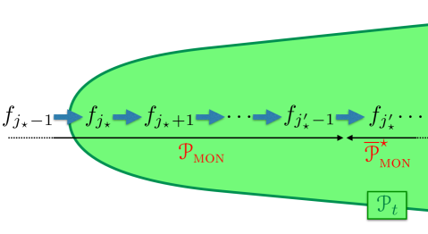
Figure 3: Proof of Theorem 14.1: we show that the sequence $\overline{{\mathcal{P}}}_{\mbox{\tiny{{mon}}}}^{\star}$ satisfies $\mathrm{Card}(\overline{{\mathcal{P}}}_{\mbox{\tiny{{mon}}}}^{\star}\cap{\mathcal{P}}_{t})\geq N$ (See text for details).

Let $f_{j_{\star}}\in{\mathcal{P}}_{t}$ be the first organism in the sequence $f_{0},f_{1},...,f_{T}$ to hit ${\mathcal{P}}_{t}$. Because of Theorem 4.2 and Lemma 4.4, with high probability, all organisms before $f_{j_{\star}}$ belong to ${\mathcal{P}}_{\mbox{\tiny{{mon}}}}$. We have two cases, either $f_{j_{\star}}\in{\mathcal{P}}_{\mbox{\tiny{{mon}}}}$ or $f_{j_{\star}}\in\overline{{\mathcal{P}}}_{\mbox{\tiny{{mon}}}}$. We know already that with high probability, as long as the mutated organism $f_{j}$ stays in ${\mathcal{P}}_{\mbox{\tiny{{mon}}}}$, its performance cannot decrease; therefore, if $f_{j_{\star}}\in{\mathcal{P}}_{\mbox{\tiny{{mon}}}}$, then all subsequent mutated organism in ${\mathcal{P}}_{\mbox{\tiny{{mon}}}}$ also belong to ${\mathcal{P}}_{t}$. What will be sufficient to show Theorem 14.1 will be to show that the sequence $\overline{{\mathcal{P}}}_{\mbox{\tiny{{mon}}}}$, clamped to its first element not before $f_{j_{\star}}$ (we call it $\overline{{\mathcal{P}}}_{\mbox{\tiny{{mon}}}}^{\star}$), satisfies

$$\mathrm{Card}(\overline{{\mathcal{P}}}_{\mbox{\tiny{{mon}}}}^{\star}\cap{\mathcal{P}}_{t}) \geq N\>\>.$$ (145)

Let $f_{j^{\prime}_{\star}}$ denote the first element of $\overline{{\mathcal{P}}}_{\mbox{\tiny{{mon}}}}^{\star}$, with therefore $j^{\prime}_{\star}\geq j_{\star}$ and $f_{j^{\prime}_{\star}-1}\in{\mathcal{P}}_{\mbox{\tiny{{mon}}}}$. Let us define $\delta\stackrel{{\scriptstyle\mathrm{.}}}{{=}}t-f_{j_{\star}}$, $\delta^{\prime\prime}\stackrel{{\scriptstyle\mathrm{.}}}{{=}}\sum_{k=1}^{N}\sigma_{k}\alpha b_{\beta(k)}$ and $\delta^{\prime}\stackrel{{\scriptstyle\mathrm{.}}}{{=}}\delta-\delta^{\prime\prime}$, $\sigma_{k}\in\{-1,1\}$ and $\beta:[N]\rightarrow[{d_{\mbox{\tiny{$\mathcal{B}$}}}}]$ gives the mutations chosen to evolve further $f_{j^{\prime}_{\star}}$ for $N$ steps. All coordinates for $\delta,\delta^{\prime},\delta^{\prime\prime},b_{\beta(k)}$ are expressed in basis $\mathcal{B}^{*}$. Using eq. (17) in Lemma 11.2 and the expression of $\mbox{{\normalsize{m}}}\succ 0$ in (16), and Lemma 11.2, we get, for any $N^{\prime}\in[N]$,

$$\mathbb{E}_{x\sim{\mathcal{D}}}\left[D_{\varphi}\left(\left(\left.f_{j^{\prime}_{\star}}+\sum_{k\in[N^{\prime}]}\sigma_{k}\alpha b_{\beta(k)}\right)(x)\right\|t(x)\right)\right] = \frac{1}{2}\cdot\langle\mbox{{\normalsize{b}}}^{*}\delta^{\prime},\mbox{{\normalsize{m}}}\mbox{{\normalsize{b}}}^{*}\delta^{\prime}\rangle$$ (146)

$$\leq \frac{\gamma^{\prime}}{2}\cdot\langle\mbox{{\normalsize{b}}}^{*}\delta^{\prime},\Psi\mbox{{\normalsize{b}}}^{*}\delta^{\prime}\rangle\>\>.$$

We then observe

$$\frac{\gamma^{\prime}}{2}\cdot\langle\mbox{{\normalsize{b}}}^{*}\delta^{\prime},\Psi\mbox{{\normalsize{b}}}^{*}\delta^{\prime}\rangle \leq \gamma^{\prime}\cdot\langle\mbox{{\normalsize{b}}}^{*}\delta,\Psi\mbox{{\normalsize{b}}}^{*}\delta\rangle+\alpha\gamma^{\prime}\cdot\langle\mbox{{\normalsize{b}}}^{*}\delta^{\prime\prime},\Psi\mbox{{\normalsize{b}}}^{*}\delta^{\prime\prime}\rangle$$ (147)

$$\leq \gamma^{\prime}\cdot\langle\mbox{{\normalsize{b}}}^{*}\delta,\Psi\mbox{{\normalsize{b}}}^{*}\delta\rangle+N^{\prime}\alpha\gamma^{\prime}\cdot\sum_{k\in[N^{\prime}]}\langle\mbox{{\normalsize{b}}}^{*}b_{\beta(k)},\Psi\mbox{{\normalsize{b}}}^{*}b_{\beta(k)}\rangle$$

$$=\gamma^{\prime}\cdot\langle\mbox{{\normalsize{b}}}^{*}\delta,\Psi\mbox{{\normalsize{b}}}^{*}\delta\rangle+N^{\prime}\alpha\gamma^{\prime}\cdot\sum_{k\in[N^{\prime}]}\mathbb{E}_{x\sim{\mathcal{D}}}[\|b_{\beta(k)}(x)\|_{2}^{2}]$$

$$\leq \frac{2\gamma^{\prime}}{\gamma}\cdot\mathbb{E}_{x\sim{\mathcal{D}}}[D_{\varphi}(f_{j^{\prime}_{\star}}(x)\|t(x))]+N^{\prime}\alpha\gamma^{\prime}\cdot\sum_{k\in[N^{\prime}]}\mathbb{E}_{x\sim{\mathcal{D}}}[\|b_{\beta(k)}(x)\|_{2}^{2}]$$ (149)

$$\leq \frac{2\gamma^{\prime}}{\gamma}\cdot\mathbb{E}_{x\sim{\mathcal{D}}}[D_{\varphi}(f_{j^{\prime}_{\star}}(x)\|t(x))]+N^{\prime}\alpha\cdot\max\{1,V\}$$ (151)

$$=\frac{2\gamma^{\prime}}{\gamma}\cdot\mathbb{E}_{x\sim{\mathcal{D}}}[D_{\varphi}(f_{j^{\prime}_{\star}}(x)\|t(x))]+\frac{N^{\prime}z_{\alpha}}{U}\epsilon$$

$$\leq \frac{2\gamma^{\prime}}{\gamma}\cdot\left(z_{\tau}+z_{\alpha}+\frac{z_{\textsc{T}}}{z_{\alpha}}\right)\cdot\epsilon+\frac{N^{\prime}z_{\alpha}}{U}\epsilon$$

$$=\left(\frac{2\gamma^{\prime}}{\gamma}\cdot\left(z_{\tau}+z_{\alpha}+\frac{z_{\textsc{T}}}{z_{\alpha}}\right)+\frac{N^{\prime}z_{\alpha}}{U}\right)\cdot\epsilon$$

$$\leq \left(\frac{2\gamma^{\prime}}{\gamma}\cdot\left(z_{\tau}+z_{\alpha}+\frac{z_{\textsc{T}}}{z_{\alpha}}\right)+\frac{Nz_{\alpha}}{U}\right)\cdot\epsilon$$ (153)

$$\leq \epsilon\>\>.$$ (154)

Ineqs (147) and (14) hold because for any inner product $\langle.,.\rangle$ and set $\{u_{1},u_{2},...,u_{M}\}$,

$$\left\langle\sum_{k\in[M]}u_{k},\sum_{k\in[M]}u_{k}\right\rangle \leq M\cdot\sum_{k\in[M]}\langle u_{k},u_{k}\rangle\>\>,$$ (155)

since right hand side minus left hand side is $\sum_{k\neq k^{\prime}}\langle u_{k}-u_{k^{\prime}},u_{k}-u_{k^{\prime}}\rangle\geq 0$. Ineq. (149) comes from Lemma 11.2. Ineq. (151) holds because of the definition of $V$ in eq. (22). Eq. (151) holds because of the definition of $\alpha$ in eq. (24). Finally, ineq. (14) holds because we know from ineq. (102) that since $f_{j^{\prime}_{\star}}\not\in{\mathcal{P}}_{\mbox{\tiny{{mon}}}}$, then $f_{j^{\prime}_{\star}}\not\in{{\mathcal{P}}}_{t,{\mathcal{D}}}$, and so

$$\mathbb{E}_{x\sim{\mathcal{D}}}[D_{\varphi}(f_{j^{\prime}_{\star}}(x)\|t(x))] \leq \left(z_{\tau}+z_{\alpha}+\frac{z_{\textsc{T}}}{z_{\alpha}}\right)\cdot\epsilon\>\>,$$ (156)

and ineq. (154) holds because $(z_{\tau},z_{\alpha},z_{\textsc{T}})\in\mathfrak{R}_{N}$ (Definition 14.1). Indeed, constraint (iii) yields equivalently

$$\frac{2\gamma^{\prime}}{\gamma}\cdot\left(z_{\alpha}^{2}+z_{\alpha}z_{\tau}+z_{\textsc{T}}\right)+\frac{Nz^{2}_{\alpha}}{U} \leq z_{\alpha}\>\>,$$

which, after dividing by $z_{\alpha}>0$ yields that the factor in front of $\epsilon$ in eq. (153) is $\leq 1$.

Hence, the moment the sequence $f_{0},f_{1},...$ hits ${\mathcal{P}}_{t}$, it shall stay inside ${\mathcal{P}}_{t}$ with high probability for at least $N$ further evolution steps. This ends the proof of Theorem 14.1.       

15 Evolution on the efficient frontier

The fact that beneficial mutations involve a mean-divergence decomposition of the expression asks for the nature of the efficient frontier, that is, the set of mutations that would minimize $\mathbb{E}_{\mathcal{D}}[\Pi_{f,i}(x)]$ subject to a fixed $\mathbb{E}_{\mathcal{D}}[\mathrm{R}_{f,i}(x)]$. This would give “nature’s best bet” against our, perhaps, modest and small ${\mathcal{B}}$. To answer this question, we consider the restricted case of Mahalanobis divergence. Let us alleviate the constraint that $b$ involves only elements from ${\mathcal{B}}$, and, for notational convenience, define $b(x)\stackrel{{\scriptstyle\mathrm{.}}}{{=}}\sum_{i=1}^{{d_{\mbox{\tiny{${\mathcal{P}}$}}}}}b^{i}g_{i}(x)$. In this case, finding the efficient frontier is solving, similarly to that of the efficient portfolio (Merton, 1972),

$$\arg\min_{b\in{\mathbb{R}}^{{d_{\mbox{\tiny{${\mathcal{P}}$}}}}}}\Pi(b) \stackrel{{\scriptstyle\mathrm{.}}}{{=}} \frac{\alpha}{2}\cdot\mathbb{E}_{\mathcal{D}}\left[\langle b(x),\mbox{{\normalsize{m}}}b(x)\rangle\right]$$ (157)

s.c. $$\left\{\begin{array}[]{rcl}\mathbb{E}_{\mathcal{D}}\left[\langle b(x),\mbox{{\normalsize{m}}}(t-f)(x)\rangle\right]&=&r\\ \langle 1_{{d_{\mbox{\tiny{${\mathcal{P}}$}}}}},b\rangle&=&n\end{array}\>\>.\right.$$ (160)

We let the “efficient frontier” denote the equation that gives $r$ as a function of $\Pi(.)$, and for that purpose generalize $\Psi$ to $\Psi_{\mbox{\tiny{$\textsc{m}$}}}\stackrel{{\scriptstyle\mathrm{.}}}{{=}}\mathbb{E}_{x\sim{\mathcal{D}}}[\mbox{{\normalsize{g}}}^{\top}_{x}\mbox{{\normalsize{m}}}\mbox{{\normalsize{g}}}_{x}]$, for any $\mbox{{\normalsize{m}}}\in{\mathbb{R}}^{d\times d}$.

Theorem 15.1

Under setting (SF), the equation of the efficient frontier is

$$r = \left\{\begin{array}[]{lcl}\frac{n\cdot\langle 1_{{d_{\mbox{\tiny{${\mathcal{P}}$}}}}},t-f\rangle}{\langle 1_{{d_{\mbox{\tiny{${\mathcal{P}}$}}}}},\Psi_{\mbox{\tiny{$\textsc{m}$}}}^{-1}1_{{d_{\mbox{\tiny{${\mathcal{P}}$}}}}}\rangle}\cdot\left(1\pm\sqrt{(\xi(t-f)-1)(\xi(b)-1)}\right)&\mbox{ if }&\langle 1_{{d_{\mbox{\tiny{${\mathcal{P}}$}}}}},t-f\rangle\neq 0\\ \pm n\cdot\sqrt{\langle 1_{{d_{\mbox{\tiny{${\mathcal{P}}$}}}}},\Psi_{\mbox{\tiny{$\textsc{m}$}}}^{-1}1_{{d_{\mbox{\tiny{${\mathcal{P}}$}}}}}\rangle\cdot\langle t-f,\Psi_{\mbox{\tiny{$\textsc{m}$}}}(t-f)\rangle\cdot\left(\xi(b)-1\right)}&\mbox{ if }&\langle 1_{{d_{\mbox{\tiny{${\mathcal{P}}$}}}}},t-f\rangle=0\end{array}\right.$$ (163)

where $\xi(u)\stackrel{{\scriptstyle\mathrm{.}}}{{=}}\langle 1_{{d_{\mbox{\tiny{${\mathcal{P}}$}}}}},\Psi_{\mbox{\tiny{$\textsc{m}$}}}^{-1}1_{{d_{\mbox{\tiny{${\mathcal{P}}$}}}}}\rangle\cdot\langle u,\Psi_{\mbox{\tiny{$\textsc{m}$}}}u\rangle/(\langle 1_{{d_{\mbox{\tiny{${\mathcal{P}}$}}}}},u\rangle)^{2}\geq 1$ (defined for $\langle 1_{{d_{\mbox{\tiny{${\mathcal{P}}$}}}}},u\rangle\neq 0$).

Proof: Let $\delta\stackrel{{\scriptstyle\mathrm{.}}}{{=}}t-f$ for short. We solve

$$\min\Pi(b) \stackrel{{\scriptstyle\mathrm{.}}}{{=}} \frac{\alpha}{2}\cdot\langle b,\Psi_{\mbox{\tiny{$\textsc{m}$}}}b\rangle$$

s.c. $$\left\{\begin{array}[]{rcl}\langle b,\Psi_{\mbox{\tiny{$\textsc{m}$}}}\delta\rangle&=&r\\ \langle 1_{{d_{\mbox{\tiny{${\mathcal{P}}$}}}}},b\rangle&=&n\end{array}\>\>,\right.$$ (166)

Letting $\lambda_{r}$ and $\lambda_{n}$ the two Lagrange multipliers for the two constraints, we obtain the first order condition $\alpha\Psi_{\mbox{\tiny{$\textsc{m}$}}}b-\lambda_{r}\Psi_{\mbox{\tiny{$\textsc{m}$}}}\delta-\alpha\lambda_{n}1=0$, i.e.,

$$b = \frac{\lambda_{r}}{\alpha}\cdot\delta+\frac{\lambda_{n}}{\alpha}\cdot\Psi_{\mbox{\tiny{$\textsc{m}$}}}^{-1}1_{{d_{\mbox{\tiny{${\mathcal{P}}$}}}}}\>\>,$$ (167)

from which we obtain, using the constraints, the following system:

$$\left\{\begin{array}[]{rcl}\alpha r&=&\lambda_{r}\cdot\langle\delta,\Psi_{\mbox{\tiny{$\textsc{m}$}}}\delta\rangle+\lambda_{n}\cdot\langle 1_{{d_{\mbox{\tiny{${\mathcal{P}}$}}}}},\delta\rangle\\ \alpha n&=&\lambda_{r}\cdot\langle 1_{{d_{\mbox{\tiny{${\mathcal{P}}$}}}}},\delta\rangle+\lambda_{n}\cdot\langle 1_{{d_{\mbox{\tiny{${\mathcal{P}}$}}}}},\Psi_{\mbox{\tiny{$\textsc{m}$}}}^{-1}1_{{d_{\mbox{\tiny{${\mathcal{P}}$}}}}}\rangle\end{array}\right.\>\>.$$ (170)

Lemma 15.1

For any symmetric positive definite m, $\Psi_{\mbox{\tiny{$\textsc{m}$}}}\succ 0$.

The lemma is a direct consequence of assumption (iii) in (SF). Lemma 15.1 yields that $\Psi_{\mbox{\tiny{$\textsc{m}$}}}$ is invertible. To simplify this system, let us denote for short:

$$P_{b} \stackrel{{\scriptstyle\mathrm{.}}}{{=}} \frac{\alpha}{2}\cdot\langle b,\Psi_{\mbox{\tiny{$\textsc{m}$}}}b\rangle\>\>,$$

$$P_{\delta} \stackrel{{\scriptstyle\mathrm{.}}}{{=}} \frac{\alpha}{2}\cdot\langle\delta,\Psi_{\mbox{\tiny{$\textsc{m}$}}}\delta\rangle\>\>,$$

$$S \stackrel{{\scriptstyle\mathrm{.}}}{{=}} \langle 1_{{d_{\mbox{\tiny{${\mathcal{P}}$}}}}},\Psi_{\mbox{\tiny{$\textsc{m}$}}}^{-1}1_{{d_{\mbox{\tiny{${\mathcal{P}}$}}}}}\rangle\>\>,$$

$$\Delta \stackrel{{\scriptstyle\mathrm{.}}}{{=}} \langle 1_{{d_{\mbox{\tiny{${\mathcal{P}}$}}}}},\delta\rangle\>\>.$$

We obtain the simplified system:

$$\left\{\begin{array}[]{rcl}\alpha r&=&\frac{2P_{\delta}}{\alpha}\cdot\lambda_{r}+\Delta\cdot\lambda_{n}\\ \alpha n&=&\Delta\cdot\lambda_{r}+S\cdot\lambda_{n}\end{array}\right.\>\>,$$ (173)

admitting the solution

$$\lambda_{r} = \frac{\alpha^{2}Sr-\alpha^{2}\Delta n}{2SP_{\delta}-\alpha\Delta^{2}}\>\>,$$ (174)

$$\lambda_{n} = \frac{2\alpha P_{\delta}n-\alpha^{2}\Delta r}{2SP_{\delta}-\alpha\Delta^{2}}\>\>.$$ (175)

We note that $2SP_{\delta}-\alpha\Delta^{2}=\alpha(\langle\delta,\Psi_{\mbox{\tiny{$\textsc{m}$}}}\delta\rangle\langle 1_{{d_{\mbox{\tiny{${\mathcal{P}}$}}}}},\Psi_{\mbox{\tiny{$\textsc{m}$}}}^{-1}1_{{d_{\mbox{\tiny{${\mathcal{P}}$}}}}}\rangle-(\langle 1_{{d_{\mbox{\tiny{${\mathcal{P}}$}}}}},\delta\rangle)^{2})\geq 0$ from Cauchy-Schwartz inequality. Suppose that $2SP_{\delta}-\alpha\Delta^{2}>0$. Multiplying eq. (167) by $\alpha\Psi_{\mbox{\tiny{$\textsc{m}$}}}b$ yields

$$2P_{b} = \lambda_{r}r+\lambda_{n}n$$

$$= \frac{\alpha^{2}Sr^{2}-\alpha^{2}\Delta nr}{2SP_{\delta}-\alpha\Delta^{2}}+\frac{2\alpha P_{\delta}n^{2}-\alpha^{2}\Delta nr}{2SP_{\delta}-\alpha\Delta^{2}}$$

$$= \frac{\alpha^{2}Sr^{2}-2\alpha^{2}\Delta nr+2\alpha P_{\delta}n^{2}}{2SP_{\delta}-\alpha\Delta^{2}}\>\>,$$

that is, $r$ is solution of

$$\alpha^{2}Sr^{2}-2\alpha^{2}\Delta nr+2(\alpha P_{\delta}n^{2}-2SP_{b}P_{\delta}+\alpha P_{b}\Delta^{2}) = 0\>\>,$$

from which

$$r = \frac{\Delta n}{S}\pm\frac{1}{\alpha S}\sqrt{\alpha^{2}\Delta^{2}n^{2}-2S(\alpha P_{\delta}n^{2}-2SP_{b}P_{\delta}+\alpha P_{b}\Delta^{2})}$$ (176)

$$= \frac{\Delta n}{S}\pm\sqrt{\left(\frac{\Delta n}{S}\right)^{2}-\frac{2}{\alpha^{2}S}(\alpha P_{\delta}n^{2}-2SP_{b}P_{\delta}+\alpha P_{b}\Delta^{2})}$$

$$= \frac{\Delta n}{S}\pm\sqrt{\left(\frac{\Delta n}{S}\right)^{2}-\left(\frac{\Delta n}{S}\right)^{2}\left(\frac{2S}{\alpha\Delta^{2}}\cdot P_{\delta}-\frac{4S^{2}}{\alpha^{2}\Delta^{2}n^{2}}\cdot P_{b}P_{\delta}+\frac{2S}{\alpha n^{2}}\cdot P_{b}\right)}$$

$$= \frac{\Delta n}{S}\cdot\left(1\pm\sqrt{1-(\xi(\delta)+\xi(b)-\xi(\delta)\cdot\xi(b))}\right)$$

$$= \frac{\Delta n}{S}\cdot\left(1\pm\sqrt{(\xi(\delta)-1)(\xi(b)-1)}\right)\>\>,$$

with, whenever $\langle 1_{{d_{\mbox{\tiny{${\mathcal{P}}$}}}}},u\rangle\neq 0$,

$$\xi(u) \stackrel{{\scriptstyle\mathrm{.}}}{{=}} \frac{\langle 1_{{d_{\mbox{\tiny{${\mathcal{P}}$}}}}},\Psi_{\mbox{\tiny{$\textsc{m}$}}}^{-1}1_{{d_{\mbox{\tiny{${\mathcal{P}}$}}}}}\rangle\langle u,\Psi_{\mbox{\tiny{$\textsc{m}$}}}u\rangle}{(\langle 1_{{d_{\mbox{\tiny{${\mathcal{P}}$}}}}},u\rangle)^{2}}$$

$$\geq 1\>\>,$$

from Cauchy-Schwartz inequality. This ends the proof of Theorem 15.1 when $\Delta\neq 0$ and $\langle\delta,\Psi_{\mbox{\tiny{$\textsc{m}$}}}\delta\rangle\langle 1_{{d_{\mbox{\tiny{${\mathcal{P}}$}}}}},\Psi_{\mbox{\tiny{$\textsc{m}$}}}^{-1}1_{{d_{\mbox{\tiny{${\mathcal{P}}$}}}}}\rangle-(\langle 1_{{d_{\mbox{\tiny{${\mathcal{P}}$}}}}},\delta\rangle)^{2}>0$.

Now, if $\Delta=0$, $r$ is solution of

$$\alpha^{2}Sr^{2}-2P_{\delta}(2SP_{b}-\alpha n^{2}) = 0\>\>.$$ (177)

Remark that $2SP_{b}-\alpha n^{2}=\alpha(\langle 1_{{d_{\mbox{\tiny{${\mathcal{P}}$}}}}},\Psi_{\mbox{\tiny{$\textsc{m}$}}}^{-1}1_{{d_{\mbox{\tiny{${\mathcal{P}}$}}}}}\rangle\langle b,\Psi_{\mbox{\tiny{$\textsc{m}$}}}b\rangle-(\langle 1_{{d_{\mbox{\tiny{${\mathcal{P}}$}}}}},b\rangle)^{2})\geq 0$ (Cauchy-Schwartz inequality and $\alpha\geq 0$), so eq. (177) always has a solution,

$$r = \pm\left(\frac{n}{S}\right)\cdot\sqrt{\frac{2SP_{\delta}}{\alpha}\cdot\left(\xi(b)-1\right)}\>\>.$$

To finish up, when $2SP_{\delta}-\alpha\Delta^{2}=0$, system (173) simplifies to

$$\left\{\begin{array}[]{rcl}\alpha Sr&=&\Delta\cdot(\Delta\cdot\lambda_{r}+S\cdot\lambda_{n})\\ \alpha n&=&\Delta\cdot\lambda_{r}+S\cdot\lambda_{n}\end{array}\right.\>\>,$$ (180)

and so $r=\Delta n/S$. We check that $2SP_{\delta}-\alpha\Delta^{2}=0$ is equivalent to stating $\xi(\delta)=1$, in which case we also check that eq. (176) becomes $r=\Delta n/S$. This ends the proof of Theorem 15.1.        The equation depends on $\Pi(b)$ since $\xi(b)=(2\langle 1_{{d_{\mbox{\tiny{${\mathcal{P}}$}}}}},\Psi_{\mbox{\tiny{$\textsc{m}$}}}^{-1}1_{{d_{\mbox{\tiny{${\mathcal{P}}$}}}}}\rangle/(\alpha n^{2}))\cdot\Pi(b)\propto\Pi(b)$. The question is now how large can $r$ be independently of the mutation process, under the constraint that the mutator picks $b\propto\alpha b^{\prime}$ with $\alpha=O(\epsilon)$ and $\langle 1_{{d_{\mbox{\tiny{${\mathcal{P}}$}}}}},b^{\prime}\rangle$ constant (call it setting “D”). This prevents this mutator to “artificially” beat ours just because of the magnitude of mutations. Let us define vectors $\ell_{l}\stackrel{{\scriptstyle\mathrm{.}}}{{=}}[\langle 1_{{d_{\mbox{\tiny{${\mathcal{P}}$}}}}},\Psi_{\mbox{\tiny{$\textsc{m}$}}}^{-1}1_{{d_{\mbox{\tiny{${\mathcal{P}}$}}}}}\rangle\>\>\langle 1_{{d_{\mbox{\tiny{${\mathcal{P}}$}}}}},t-f\rangle]^{\top}$, $\ell_{r}\stackrel{{\scriptstyle\mathrm{.}}}{{=}}[\langle 1_{{d_{\mbox{\tiny{${\mathcal{P}}$}}}}},t-f\rangle\>\>\langle t-f,\Psi_{\mbox{\tiny{$\textsc{m}$}}}(t-f)\rangle]^{\top}$ and $\ell_{*}\stackrel{{\scriptstyle\mathrm{.}}}{{=}}[n\>\>r]^{\top}$. We also put in (D) the constraint $\xi(t-f)>1$ (implying $\det[\ell_{l}|\ell_{r}]\neq 0$), and the fact that the decomposition $\ell_{*}\stackrel{{\scriptstyle\mathrm{.}}}{{=}}v_{l}\ell_{l}+v_{r}\ell_{r}$ satisfies $|v_{l}|+|v_{r}|=O(\mathrm{tr}{[\ell_{l}|\ell_{r}]})$. This implies in particular that $n,r$ cannot be significantly larger than $\|t-f_{0}\|^{2}_{{d_{\mbox{\tiny{${\mathcal{P}}$}}}}}$, and so nature cannot have the organism “jump” from far ($f_{0}$) to close to target ($t$) in just one or few mutations.

Lemma 15.2

Under settings (SF + D), returns on the efficient frontier satisfy $r=\tilde{O}(\epsilon)$.

Proof: (We prove an explicit bound without the tilde notation) We shall prove the more explicit bound that $r=O(\uprho(t-f_{0})\cdot\epsilon)$, with (here, $x\vee y\stackrel{{\scriptstyle\mathrm{.}}}{{=}}\max\{x,y\}$)

$$\uprho(u) \stackrel{{\scriptstyle\mathrm{.}}}{{=}} |\langle 1_{{d_{\mbox{\tiny{${\mathcal{P}}$}}}}},u\rangle|{d_{\mbox{\tiny{${\mathcal{P}}$}}}}\cdot\left(\frac{\gamma^{\prime}\mu^{\prime}}{\gamma\mu}\right)^{\frac{5}{2}}\cdot\left(1\vee\left(\frac{1}{\gamma^{\prime}\mu^{\prime}}\right)+\frac{\gamma\mu\|u\|_{{d_{\mbox{\tiny{${\mathcal{P}}$}}}}}}{\sqrt{{d_{\mbox{\tiny{${\mathcal{P}}$}}}}}}\cdot 1\vee\left(\frac{\|u\|_{{d_{\mbox{\tiny{${\mathcal{P}}$}}}}}}{\sqrt{{d_{\mbox{\tiny{${\mathcal{P}}$}}}}}}\right)\right)^{2}\>\>.$$

Let us define for short $0<\psi_{\min}\leq\psi_{\max}$ the minimal and maximal eigenvalues of $\Psi_{\mbox{\tiny{$\textsc{m}$}}}$. Let $\delta\stackrel{{\scriptstyle\mathrm{.}}}{{=}}t-f$ for short and column vectors

$$\ell_{l}=\left[\begin{array}[]{c}\langle 1_{{d_{\mbox{\tiny{${\mathcal{P}}$}}}}},\Psi_{\mbox{\tiny{$\textsc{m}$}}}^{-1}1_{{d_{\mbox{\tiny{${\mathcal{P}}$}}}}}\rangle\\ \langle 1_{{d_{\mbox{\tiny{${\mathcal{P}}$}}}}},\delta\rangle\end{array}\right]\>\>,\ell_{r}=\left[\begin{array}[]{c}\langle 1_{{d_{\mbox{\tiny{${\mathcal{P}}$}}}}},\delta\rangle\\ \langle\delta,\Psi_{\mbox{\tiny{$\textsc{m}$}}}\delta\rangle\\ \end{array}\right]\>\>,\ell_{*}=\left[\begin{array}[]{c}n\\ r\end{array}\right]\>\>.$$ (187)

Since $\langle 1_{{d_{\mbox{\tiny{${\mathcal{P}}$}}}}},\Psi_{\mbox{\tiny{$\textsc{m}$}}}^{-1}1_{{d_{\mbox{\tiny{${\mathcal{P}}$}}}}}\rangle\leq{d_{\mbox{\tiny{${\mathcal{P}}$}}}}/\psi_{\min}$ and $\langle b,\Psi_{\mbox{\tiny{$\textsc{m}$}}}b\rangle\leq\psi_{\max}\|b\|^{2}_{{d_{\mbox{\tiny{${\mathcal{P}}$}}}}}$, we have

$$\xi(b) = \frac{\langle 1_{{d_{\mbox{\tiny{${\mathcal{P}}$}}}}},\Psi_{\mbox{\tiny{$\textsc{m}$}}}^{-1}1_{{d_{\mbox{\tiny{${\mathcal{P}}$}}}}}\rangle\langle b,\Psi_{\mbox{\tiny{$\textsc{m}$}}}b\rangle}{n^{2}}$$

$$\leq \frac{{d_{\mbox{\tiny{${\mathcal{P}}$}}}}\psi_{\max}}{n^{2}\psi_{\min}}\cdot\|b\|^{2}_{{d_{\mbox{\tiny{${\mathcal{P}}$}}}}}\>\>.$$

We have also from eq. (167),

$$\|b\|^{2}_{{d_{\mbox{\tiny{${\mathcal{P}}$}}}}} = \frac{\lambda^{2}_{r}}{\alpha^{2}}\cdot\|\delta\|^{2}_{{d_{\mbox{\tiny{${\mathcal{P}}$}}}}}+\frac{2\lambda_{r}\lambda_{n}}{\alpha^{2}}\cdot\langle\delta,\Psi_{\mbox{\tiny{$\textsc{m}$}}}^{-1}1_{{d_{\mbox{\tiny{${\mathcal{P}}$}}}}}\rangle+\frac{\lambda^{2}_{n}}{\alpha^{2}}\cdot\langle 1_{{d_{\mbox{\tiny{${\mathcal{P}}$}}}}},\Psi_{\mbox{\tiny{$\textsc{m}$}}}^{-2}1_{{d_{\mbox{\tiny{${\mathcal{P}}$}}}}}\rangle\>\>.$$ (188)

It comes from eqs (174, 175),

$$\frac{\lambda^{2}_{r}}{\alpha^{2}} = \frac{\alpha^{2}(\langle 1_{{d_{\mbox{\tiny{${\mathcal{P}}$}}}}},\Psi_{\mbox{\tiny{$\textsc{m}$}}}^{-1}1_{{d_{\mbox{\tiny{${\mathcal{P}}$}}}}}\rangle\cdot r-\langle 1_{{d_{\mbox{\tiny{${\mathcal{P}}$}}}}},\delta\rangle\cdot n)^{2}}{(\langle 1_{{d_{\mbox{\tiny{${\mathcal{P}}$}}}}},\Psi_{\mbox{\tiny{$\textsc{m}$}}}^{-1}1_{{d_{\mbox{\tiny{${\mathcal{P}}$}}}}}\rangle\langle\delta,\Psi_{\mbox{\tiny{$\textsc{m}$}}}\delta\rangle-(\langle 1_{{d_{\mbox{\tiny{${\mathcal{P}}$}}}}},\delta\rangle)^{2})^{2}}\>\>,$$

$$= \frac{\alpha^{2}\det^{2}[\ell_{l}|\ell_{*}]}{\det^{2}[\ell_{l}|\ell_{r}]}\>\>,$$

$$\frac{\lambda_{r}\lambda_{n}}{\alpha^{2}} = \frac{\alpha^{2}\det[\ell_{l}|\ell_{*}]\det[\ell_{*}|\ell_{r}]}{\det^{2}[\ell_{l}|\ell_{r}]}\>\>,$$

$$\frac{\lambda^{2}_{n}}{\alpha^{2}} = \frac{\alpha^{2}\det^{2}[\ell_{*}|\ell_{r}]}{\det^{2}[\ell_{l}|\ell_{r}]}\>\>.$$

Using the fact that $\langle\delta,\Psi_{\mbox{\tiny{$\textsc{m}$}}}^{-1}1_{{d_{\mbox{\tiny{${\mathcal{P}}$}}}}}\rangle\leq\sqrt{{d_{\mbox{\tiny{${\mathcal{P}}$}}}}}\|\delta\|_{{d_{\mbox{\tiny{${\mathcal{P}}$}}}}}/\psi_{\min}$ and $\langle 1_{{d_{\mbox{\tiny{${\mathcal{P}}$}}}}},\Psi_{\mbox{\tiny{$\textsc{m}$}}}^{-2}1_{{d_{\mbox{\tiny{${\mathcal{P}}$}}}}}\rangle\leq{d_{\mbox{\tiny{${\mathcal{P}}$}}}}/\psi_{\min}^{2}$, we obtain from eq. (188)

$$\xi(b) \leq \frac{{d_{\mbox{\tiny{${\mathcal{P}}$}}}}\psi_{\max}}{\psi_{\min}}\cdot\left(\frac{\alpha}{n}\right)^{2}\cdot\left(\frac{\psi_{\min}\|\delta\|_{{d_{\mbox{\tiny{${\mathcal{P}}$}}}}}\cdot\det[\ell_{l}|\ell_{*}]+\sqrt{{d_{\mbox{\tiny{${\mathcal{P}}$}}}}}\cdot\det[\ell_{*}|\ell_{r}]}{\psi_{\min}\cdot\det[\ell_{l}|\ell_{r}]}\right)^{2}\>\>.$$ (189)

Let $v_{l},v_{r}$ be such that $\ell_{*}=v_{l}\cdot\ell_{l}+v_{r}\cdot\ell_{r}$. Such reals are guaranteed to exist since $\det[\ell_{l}|\ell_{r}]=\langle 1_{{d_{\mbox{\tiny{${\mathcal{P}}$}}}}},\Psi_{\mbox{\tiny{$\textsc{m}$}}}^{-1}1_{{d_{\mbox{\tiny{${\mathcal{P}}$}}}}}\rangle\cdot\langle\delta,\Psi_{\mbox{\tiny{$\textsc{m}$}}}\delta\rangle-(\langle 1_{{d_{\mbox{\tiny{${\mathcal{P}}$}}}}},\delta\rangle)^{2}\neq 0$ by assumption. Then $\det[\ell_{*}|\ell_{r}]=v_{l}\cdot\det[\ell_{l}|\ell_{r}]$ and $\det[\ell_{l}|\ell_{*}]=v_{r}\cdot\det[\ell_{l}|\ell_{r}]$. We get

$$\xi(b) \leq \frac{{d_{\mbox{\tiny{${\mathcal{P}}$}}}}\psi_{\max}}{\psi_{\min}}\cdot\left(\frac{\alpha}{n}\right)^{2}\cdot\left(\frac{\sqrt{{d_{\mbox{\tiny{${\mathcal{P}}$}}}}}}{\psi_{\min}}+\|\delta\|_{{d_{\mbox{\tiny{${\mathcal{P}}$}}}}}\right)^{2}\cdot\left(\frac{|\det[\ell_{l}|\ell_{*}]|+|\det[\ell_{*}|\ell_{r}]|}{\det[\ell_{l}|\ell_{r}]}\right)^{2}$$ (190)

$$=\frac{{d_{\mbox{\tiny{${\mathcal{P}}$}}}}\psi_{\max}}{\psi_{\min}}\cdot\left(\frac{\alpha}{n}\right)^{2}\cdot\left(\frac{\sqrt{{d_{\mbox{\tiny{${\mathcal{P}}$}}}}}}{\psi_{\min}}+\|\delta\|_{{d_{\mbox{\tiny{${\mathcal{P}}$}}}}}\right)^{2}\cdot\left(|v_{l}|+|v_{r}|\right)^{2}$$

$$\leq \frac{{d_{\mbox{\tiny{${\mathcal{P}}$}}}}\psi_{\max}}{\psi_{\min}}\cdot\left(\frac{\alpha}{n}\right)^{2}\cdot\left(\frac{\sqrt{{d_{\mbox{\tiny{${\mathcal{P}}$}}}}}}{\psi_{\min}}+\|\delta\|_{{d_{\mbox{\tiny{${\mathcal{P}}$}}}}}\right)^{2}\cdot\left(\frac{{d_{\mbox{\tiny{${\mathcal{P}}$}}}}}{\psi_{\min}}+\psi_{\max}\|\delta\|^{2}_{{d_{\mbox{\tiny{${\mathcal{P}}$}}}}}\right)^{2}\>\>.$$

The last inequality comes from assumption (D), since

$$\mathrm{tr}{[\ell_{l}|\ell_{r}]} = \langle 1_{{d_{\mbox{\tiny{${\mathcal{P}}$}}}}},\Psi_{\mbox{\tiny{$\textsc{m}$}}}^{-1}1_{{d_{\mbox{\tiny{${\mathcal{P}}$}}}}}\rangle+\langle\delta,\Psi_{\mbox{\tiny{$\textsc{m}$}}}\delta\rangle$$

$$\leq \frac{{d_{\mbox{\tiny{${\mathcal{P}}$}}}}}{\psi_{\min}}+\psi_{\max}\|\delta\|^{2}_{{d_{\mbox{\tiny{${\mathcal{P}}$}}}}}\>\>.$$

If $n=\theta(\alpha)$, then the dependence in the magnitude of mutations disappear and, taking the square root in ineq. (190),

$$\sqrt{\xi(b)} = O\left(\sqrt{\frac{{d_{\mbox{\tiny{${\mathcal{P}}$}}}}\psi_{\max}}{\psi_{\min}}}\left(\frac{\sqrt{{d_{\mbox{\tiny{${\mathcal{P}}$}}}}}}{\psi_{\min}}+\|\delta\|_{{d_{\mbox{\tiny{${\mathcal{P}}$}}}}}\right)\cdot\left(\frac{{d_{\mbox{\tiny{${\mathcal{P}}$}}}}}{\psi_{\min}}+\psi_{\max}\|\delta\|^{2}_{{d_{\mbox{\tiny{${\mathcal{P}}$}}}}}\right)\right)\>\>,$$ (191)

out of which we get, assuming $\langle 1_{{d_{\mbox{\tiny{${\mathcal{P}}$}}}}},\delta\rangle\neq 0$, the following upperbound for returns on the efficient frontier:

$$r = O\left\{\frac{|\langle 1_{{d_{\mbox{\tiny{${\mathcal{P}}$}}}}},\delta\rangle|\psi_{\max}}{{d_{\mbox{\tiny{${\mathcal{P}}$}}}}}\cdot\left(1+\sqrt{\frac{{d_{\mbox{\tiny{${\mathcal{P}}$}}}}\psi_{\max}}{\psi_{\min}}}\left(\frac{\sqrt{{d_{\mbox{\tiny{${\mathcal{P}}$}}}}}}{\psi_{\min}}+\|\delta\|_{{d_{\mbox{\tiny{${\mathcal{P}}$}}}}}\right)\cdot\left(\frac{{d_{\mbox{\tiny{${\mathcal{P}}$}}}}}{\psi_{\min}}+\psi_{\max}\|\delta\|^{2}_{{d_{\mbox{\tiny{${\mathcal{P}}$}}}}}\right)\right)\cdot\epsilon\right\}$$

$$= O\left\{|\langle 1_{{d_{\mbox{\tiny{${\mathcal{P}}$}}}}},\delta\rangle|\cdot\left(\frac{\psi_{\max}}{\psi_{\min}}\right)^{\frac{3}{2}}\cdot\left(1+\frac{\psi_{\min}\|\delta\|_{{d_{\mbox{\tiny{${\mathcal{P}}$}}}}}}{\sqrt{{d_{\mbox{\tiny{${\mathcal{P}}$}}}}}}\right)\cdot\left(\frac{{d_{\mbox{\tiny{${\mathcal{P}}$}}}}}{\psi_{\min}}+\psi_{\max}\|\delta\|^{2}_{{d_{\mbox{\tiny{${\mathcal{P}}$}}}}}\right)\cdot\epsilon\right\}$$

$$= O\left\{|\langle 1_{{d_{\mbox{\tiny{${\mathcal{P}}$}}}}},\delta\rangle|{d_{\mbox{\tiny{${\mathcal{P}}$}}}}\cdot\left(\frac{\psi_{\max}}{\psi_{\min}}\right)^{\frac{5}{2}}\cdot\left(1+\frac{\psi_{\min}\|\delta\|_{{d_{\mbox{\tiny{${\mathcal{P}}$}}}}}}{\sqrt{{d_{\mbox{\tiny{${\mathcal{P}}$}}}}}}\right)\cdot\left(\frac{1}{\psi_{\max}}+\frac{\psi_{\min}\|\delta\|^{2}_{{d_{\mbox{\tiny{${\mathcal{P}}$}}}}}}{{d_{\mbox{\tiny{${\mathcal{P}}$}}}}}\right)\cdot\epsilon\right\}$$

$$= O\left\{|\langle 1_{{d_{\mbox{\tiny{${\mathcal{P}}$}}}}},\delta\rangle|{d_{\mbox{\tiny{${\mathcal{P}}$}}}}\cdot\left(\frac{\psi_{\max}}{\psi_{\min}}\right)^{\frac{5}{2}}\cdot\left(1\vee\left(\frac{1}{\psi_{\max}}\right)+\frac{\psi_{\min}\|\delta\|_{{d_{\mbox{\tiny{${\mathcal{P}}$}}}}}}{\sqrt{{d_{\mbox{\tiny{${\mathcal{P}}$}}}}}}\cdot 1\vee\left(\frac{\|\delta\|_{{d_{\mbox{\tiny{${\mathcal{P}}$}}}}}}{\sqrt{{d_{\mbox{\tiny{${\mathcal{P}}$}}}}}}\right)\right)^{2}\cdot\epsilon\right\}\>\>.$$

We then conclude, noting that we can fix $\psi_{\min}=\gamma\mu$ and $\psi_{\max}=\gamma^{\prime}\mu^{\prime}$.        Hence, in the (D) regime, the mutation mechanism on the efficient frontier enjoys a dependence on $\epsilon$ of the same order as that of superior beneficial mutations, that always exist in $\mathcal{B}$ under setting (SF) alone — if we modify our mutator so that it picks the best mutation at each iteration, like $\mathsf{Opt\mbox{-}Sel}$ in (Angelino and Kanade, 2014), then we are guaranteed to have mutations with a near-optimal dependence in $\epsilon$ throughout all ${\mathcal{P}}_{\mbox{\tiny{{mon}}}}$.

16 Toy experiments (full)

	Performance plots	Evolution in the ambient space
Unsupervised
Supervised

Table 3: Experiments on toy domains for unsupervised (top) and supervised learning (bottom). Left plots: performances, indicating the $-\epsilon$ evolvability threshold in green. In the case of supervised learning, the data (right: black = positive class, grey = negative class) are not linearly separable, so we compute the performance minus that of the optimal linear separator (eq. (12)). Right plots: data and organisms evolved. Organisms are displayed in cyan and dark blue. Dark blue means that the organism satisfies the condition of the evolvability model (eqs. (3) for top, (12) for bottom). A red dot (top) and red vector (down) display the target. Top right: green dots are estimates of the target used for evolution. Bottom right: the last vector evolved is displayed with a dark blue line; it is almost confounded with the target.

Algorithm 2 $\mathsf{Simple\mbox{-}Evol}$($\mathcal{S}$)

  Input: sample $\mathcal{S}$;

  Initialize $f\leftarrow f_{0}$;

  For $t=0,1,...,T-1$

  Step $t$.1: if $t\%1000=0$ then $\mathcal{B}\leftarrow\mathsf{Gen}(\mathcal{S})$;

  Step $t$.2: Compute $\textsc{Bene}(f_{t})$ and $\textsc{Neut}(f_{t})$ using $\textsc{n}_{\epsilon}(f_{t})$ as in (4)

  Step $t$.3: if $\textsc{Bene}(f_{t})\neq\emptyset$ then $f_{t+1}\sim_{\mathrm{unif.}}\textsc{Bene}(f_{t})$;

      else if $\textsc{Neut}(f_{t})\neq\emptyset$ then $f_{t+1}\sim_{\mathrm{unif.}}\textsc{Neut}(f_{t})$;

      else $f_{t+1}\sim_{\mathrm{unif.}}\textsc{n}_{\epsilon}(f_{t})$;

  Return $f_{T}$;

The high-level implementation of the algorithm, $\mathsf{Simple\mbox{-}Evol}$, is sketched in Algorithm 2 ($\mathsf{Gen}(\mathcal{S})$ returns a random set from $\mathcal{S}$ that generates ${\mathbb{R}}^{2}$). Details of the experiments are as follows.

$\hookrightarrow$ Supervised learning: we generate a mixture of 2D spherical Gaussians with random variance and a random number of vectors in each; vectors of each Gaussian are all labeled positive (black) or negative (grey, class picked uniformly at random). The data is not linearly separable, so the optimal linear separator does not have zero error, and we are in the agnostic setting of Theorem 5.1. The performance chosen is (minus) the square loss. To speed the mutator, we threshold the number $m$ of conditions sampled at each iteration to a maximum of $50000$.
$\hookrightarrow$ Unsupervised learning: to guarantee an optimum that can be measured and compared with, the problem is the estimation of a sample mean. The performance of an organism $f$ with respect to target $\hat{\mu}$ is $\texttt{Perf}_{\mu,\varphi}(f,{\mathcal{S}})\stackrel{{\scriptstyle\mathrm{.}}}{{=}}-\|f-\hat{\mu}_{\mathcal{S}}\|_{2}^{2}$. Notice that the target is the distribution’s expectation. To complicate this easy task, we restrict the computation of $\hat{\mu}_{\mathcal{S}}$ over 5 vectors chosen at random in the data. Hence, while the expectation of $\hat{\mu}_{\mathcal{S}}$ is still the sample’s expectation, the variance of $\hat{\mu}_{\mathcal{S}}$ is large. In Table 3 (top right), the small green dots display the $\hat{\mu}_{\mathcal{S}}$ picked. They spread on a large portion of the domain around the target.

In both supervised and unsupervised experiments, all data are normalized to fit in a disk of unit norm. we implement the mutator and all other parameters as they are given above, picking $\epsilon=\frac{1}{10}$ and $\mathcal{B}$ consisting of two randomly chosen vectors in the data that generate ${\mathbb{R}}^{2}$, flipped to get four mutations. Each 1000 evolvability steps, we renew the basis, still completely at random. Sometimes, in particular for the supervised experiment, both Bene and Neut are empty. In this case of “failure”, we just force evolution’s hand by taking one of the mutants, chosen uniformly at random in the neighborhood. Therefore, there is not other optimization process carried out in our implementation than the weak optimization achieved by the mutator.

References

- Amari and Nagaoka (2000) S.-I. Amari and H. Nagaoka. Methods of Information Geometry. Oxford University Press, 2000.
- Angelino and Kanade (2014) E. Angelino and V. Kanade. Attribute-efficient evolvability of linear functions. CoRR, abs/1309.4132v2, 2014.
- Banerjee et al. (2005a) A. Banerjee, X. Guo, and H. Wang. On the optimality of conditional expectation as a Bregman predictor. IEEE Trans. on Information Theory, 51:2664–2669, 2005a.
- Banerjee et al. (2005b) A. Banerjee, S. Merugu, I. Dhillon, and J. Ghosh. Clustering with Bregman divergences. Journal of Machine Learning Research, 6:1705–1749, 2005b.
- Blute (2016) M. Blute. Evolution and learning: A response to Watson and Szathmáry. Trends in Ecology and Evolution, 31:891–892, 2016.
- Boissonnat et al. (2010) J.-D. Boissonnat, F. Nielsen, and R. Nock. Bregman Voronoi diagrams. DCG, 44(2):281–307, 2010.
- Bregman (1967) L. M. Bregman. The relaxation method of finding the common point of convex sets and its application to the solution of problems in convex programming. USSR Comp. Math. and Math. Phys., 7:200–217, 1967.
- Conn et al. (2008) A.-R. Conn, K. Scheinberg, and L.-N. Vicente. Introduction to Derivative-Free Optimization. SIAM, 2008.
- Diochnos and Turán (2009) D.-I. Diochnos and G. Turán. On evolvability: The swapping algorithm, product distributions, and covariance. In 5th SAGA, pages 74–88, 2009.
- Feldman (2008) V. Feldman. Evolvability from learning algorithms. In Proc. of the 41 ACM Symposium on the Theory of Computing, pages 619–628, 2008.
- Feldman (2009) V. Feldman. Robustness of evolvability. In Proc. of the 22 COLT, 2009.
- Feldman (2011) V. Feldman. Distribution-independent evolvability of linear threshold functions. In Proc. of the 24 COLT, pages 253–272, 2011.
- Feldman (2012) V. Feldman. A complete characterization of statistical query learning with applications to evolvability. J. Comp. Syst. Sc., 78:1444–1459, 2012.
- Griewank (1981) A.-O. Griewank. Generalized decent for global optimization. Journal of Optimization Theory and Applications, 34:11–39, 1981.
- Hartwell et al. (1999) L.-H. Hartwell, J.-J. Hopfield, S. Leibler, and A. W. Murray. From molecular to modular cell biology. Nature, 402:47–52, 1999.
- Jordán (2016) F. Jordán. How can mature ecosystems become educated? a response to Watson and Szathmáry. Trends in Ecology and Evolution, 31:893–894, 2016.
- Kafri et al. (2009) R. Kafri, M. Springer, and Y. Pilpel. Genetic redundancy: New tricks for old genes. Cell, pages 389–392, 2009.
- Kanade et al. (2010) V. Kanade, L.-G. Valiant, and J. Wortman Vaughan. Evolution with drifting targets. In Proc. of the 23 COLT, pages 155–167, 2010.
- Kitano (2010) H. Kitano. Violations of robustness tradeoffs. Molecular Systems Biology, page 384, 2010.
- Livnat and Papadimitriou (2016) A. Livnat and C. Papadimitriou. Evolution and learning: Used together, fused together. Trends in Ecology and Evolution, 31:894–896, 2016.
- Markowitz (1952) H. Markowitz. Portfolio selection. Journal of Finance, 6:77–91, 1952.
- McDiarmid (1998) C. McDiarmid. Concentration. In M. Habib, C. McDiarmid, J. Ramirez-Alfonsin, and B. Reed, editors, Probabilistic Methods for Algorithmic Discrete Mathematics, pages 1–54. Springer Verlag, 1998.
- Merton (1972) R. Merton. An analytic derivation of the efficient portfolio frontier. J. of Financial and Quantitative Analysis, 7:1851–1872, 1972.
- Michael (2012) L. Michael. Evolvability via the Fourier transform. Theoretical Computer Science, 462:88–98, 2012.
- Nelder and Mead (1965) J.-A. Nelder and R. Mead. Simplex method for function minimization. Computer Journal, 7:308–313, 1965.
- Nesterov and Spokoiny (2017) Y. Nesterov and V. Spokoiny. Random gradient-free optimization of convex functions. Foundations of Computational Mathematics, 17:527–566, 2017.
- Nock and Nielsen (2008) R. Nock and F. Nielsen. On the efficient minimization of classification-calibrated surrogates. In NIPS*21, pages 1201–1208, 2008.
- Pekkonen et al. (2013) M. Pekkonen, T. Ketola, and J.-T. Laakso. Resource availability and competition shape the evolution of survival and growth ability in a bacterial community. PLoS ONE, 2013.
- Reid and Williamson (2010) M.-D. Reid and R.-C. Williamson. Composite binary losses. Journal of Machine Learning Research, 11, 2010.
- Schwenk and Wagner (2015) K. Schwenk and G.-P. Wagner. Function and the evolution of phenotypic stability: connecting pattern to process. Integrative and Comparative Biology, 563(3):552–563, 2015.
- Stearns (2010) F.-W. Stearns. One hundred years of pleiotropy: A retrospective. Genetics, pages 767–773, 2010.
- Valiant (2009) L. G. Valiant. Evolvability. Communications of the ACM, 51(1), 2009.
- Valiant (2014) P. Valiant. Evolvability of real functions. ACM Trans. on Computation Theory, 6:12:3–12:19, 2014.
- Watson and Szathmáry (2016a) R.-A. Watson and E. Szathmáry. How can evolution learn ? Trends in Ecology and Evolution, 31:147–157, 2016a.
- Watson and Szathmáry (2016b) R.-A. Watson and E. Szathmáry. How can evolution learn ? — a reply to responses. Trends in Ecology and Evolution, 31:896–897, 2016b.
- Žliobaitė and Stenseth (2016) I. Žliobaitė and N.-C. Stenseth. Improving adaptation through learning: a response to Watson and Szathmáry. Trends in Ecology and Evolution, 31:892–893, 2016.