Computing and Graphing Probability Values of Pearson Distributions: A SAS/IML Macro

Abstract

Any empirical data can be approximated to one of Pearson distributions using the first four moments of the data (Elderton and Johnson, 1969; Pearson, 1895; Solomon and Stephens, 1978). Thus, Pearson distributions made statistical analysis possible for data with unknown distributions. There are both extant old-fashioned in-print tables (Pearson and Hartley, 1972) and contemporary computer programs (Amos and Daniel, 1971; Bouver and Bargmann, 1974; Bowman and Shenton, 1979; Davis and Stephens, 1983; Pan, 2009) available for obtaining percentage points of Pearson distributions corresponding to certain pre-specified percentages (or probability values) (e.g., 1.0%, 2.5%, 5.0%, etc.), but they are little useful in statistical analysis because we have to rely on unwieldy second difference interpolation to calculate a probability value of a Pearson distribution corresponding to any given percentage point, such as an observed test statistic in hypothesis testing. Thus, the present study develops a SAS/IML macro program to compute and graph probability values of Pearson distributions for any given percentage point so as to facilitate researchers to conduct statistical analysis on data with unknown distributions.

Keywords: Pearson distributions, curve fitting; distribution-free statistics; hypothesis testing

1 Introduction

Most of statistical analysis relies on normal distributions, but this assumption is often difficult to meet in reality. Pearson distributions can be approximated for any data using the first four moments of the data (Elderton and Johnson, 1969; Pearson, 1895; Solomon and Stephens, 1978). Thus, Pearson distributions made statistical analysis possible for any data with unknown distributions. For instance, in hypothesis testing, a sampling distribution of an observed test statistic is usually unknown but the sampling distribution can be fitted into one of Pearson distributions. Then, we can compute and use a p-value (or probability value) of the approximated Pearson distribution to make a statistical decision for such distribution-free hypothesis testing.

There are both extant old-fashioned in-print tables (Pearson and Hartley, 1972) and contemporary computer programs (Amos and Daniel, 1971; Bouver and Bargmann, 1974; Bowman and Shenton, 1979; Davis and Stephens, 1983; Pan, 2009) that provided a means of obtaining percentage points of Pearson distributions corresponding to certain pre-specified percentages (or probability values) (e.g., 1.0%, 2.5%, 5.0%, etc.). Unfortunately, they are little useful in statistical analysis because we have to employ unwieldy second difference interpolation for both skewness $\surd\beta_{1}$ and kurtosis $\beta_{2}$ to calculate a probability value of a Pearson distribution corresponding to any given percentage point, such as an observed test statistic in hypothesis testing. Thus, a new program is needed for easily computing probability values of Pearson distributions for any given probability values; and therefore, researchers can utilize the program to conduct more applicable statistical analysis, such as distribution-free hypothesis testing, on data with unknown distributions.

2 Pearson distributions

Pearson distributions are a family of distributions which consist of seven different types of distributions plus normal distribution (Table 1). Let $X$ represent given data, once its first four moments are calculated by

$$\left\{\begin{array}[]{l}\mu_{1}^{\prime}=E(X);\\ \mu_{i}=E[X-E(X)]^{i}=E[X-\mu_{1}^{\prime}]^{i},i=2,3,4,\end{array}\right.$$ (1)

types of Pearson distributions to which $X$ will be approximated can be determined by a $\kappa$-criterion that is defined as follows (Elderton and Johnson, 1969):

$$\kappa=\frac{\beta_{1}(\beta_{2}+3)^{2}}{4(4\beta_{2}-3\beta_{1})(2\beta_{2}-3\beta_{1}-6)},$$ (2)

where the $\beta$-coefficients (i.e., skewness and kurtosis) are calculated as follows:

$$\left\{\begin{array}[]{l}\surd\beta_{1}=\frac{\mu_{3}}{\mu_{2}^{3/2}}\mbox{ (also }\beta_{1}=(\surd\beta_{1})^{2}=\frac{\mu_{3}^{2}}{\mu_{2}^{3}});\\ \beta_{2}=\frac{\mu_{4}}{\mu_{2}^{2}}.\end{array}\right.$$ (3)

Type	$\kappa$-Criterion	Density Function	Domain
Main Type
I	$\kappa<0$	$f(x)=y_{0}(1+\frac{x}{a_{1}})^{m_{1}}(1-\frac{x}{a_{2}})^{m_{2}}$	$-a_{1}\leq x\leq a_{2}$
IV	$0<\kappa<1$	$f(x)=y_{0}(1+\frac{x^{2}}{a^{2}})^{-m}e^{-\nu\arctan(x/a)}$	$-\infty<x<\infty$
VI	$\kappa>1$	$f(x)=y_{0}(x-a)^{q_{2}}x^{-q_{1}}$	$a\leq x<\infty$
Transition Type
Normal	$\kappa=0\mbox{ }(\beta_{2}=3)$	$f(x)=y_{0}e^{-x^{2}/(2\mu_{2})}$	$-\infty<x<\infty$
II	$\kappa=0\mbox{ }(\beta_{2}<3)$	$f(x)=y_{0}(1-\frac{x^{2}}{a^{2}})^{m}$	$-a\leq x\leq a$
III	$\kappa=\pm\infty$	$f(x)=y_{0}(1+\frac{x}{a})^{\gamma{a}}e^{-\gamma{x}}$	$-a\leq x<\infty$
V	$\kappa=1$	$f(x)=y_{0}x^{-p}e^{-\gamma/x}$	$0<x<\infty$
VII	$\kappa=0\mbox{ }(\beta_{2}>3)$	$f(x)=y_{0}(1+\frac{x^{2}}{a^{2}})^{-m}$	$-\infty<x<\infty$

Table 1: Types of Pearson distributions.

The determination of types of Pearson distributions by the $\kappa$-criterion (Equation 2) is illustrated in Table 1. From Table 1, we can also see that for each type of Pearson distributions, its density function has a closed form with a clearly defined domain of $X$. The closed form of density functions made numerical integration possible for obtaining probability values of approximated Pearson distributions. Following the calculation formulas introduced in Elderton and Johnson (1969), the parameters (e.g., $y_{0}$, $m_{1}$, $m_{2}$, $a_{1}$, $a_{2}$, etc.) of the density functions will be automatically computed in a SAS/IML (SAS Institute Inc., 2011) macro program described in the next section. Then, probability values of Pearson distributions can be obtained through numerical integration with the SAS subroutine QUAD.

3 A SAS/IML macro program

The main SAS/IML macro program to compute and graph probability values of Pearson distributions is as follows:

%PearsonProb(mu2 = , mu3 = , mu4 = , x0 = , plot = )

where

• mu2 = the second moment $\mu_{2}$;

• mu3 = the third moment $\mu_{3}$;

• mu4 = the fourth moment $\mu_{4}$;

• x0 = the percentage point $x_{0}$;

• plot = 1 for graph, 0 for no graph.

It is worth noting that the first moment $\mu_{1}^{\prime}$ is not an input value for this macro and that only the second, the third, and the fourth moments as well as a percentage point $x_{0}$ and 1 or 0 for plot are required. The reason is that the first moment $\mu_{1}^{\prime}$ has been already included in the calculation for the higher-oder moments (see Equation 1).

This SAS/IML macro program starts with computing $\beta$-coefficients defined in Equation 3 using the inputed values of $\mu_{2}$, $\mu_{3}$, $\mu_{4}$, and $x_{0}$. Then, plug them into Equation 2 to calculate $\kappa$. Based on the value of the $\kappa$, a specific type of Pearson distribution is determined by the $\kappa$-criterion displayed in Table 1, followed by calculations of the parameters (e.g., $y_{0}$, $m_{1}$, $m_{2}$, $a_{1}$, $a_{2}$, etc.) for the density function of the specific type of Pearson distribution listed in Table 1. To compute the probability value of the specific Pearson distribution corresponding to the inputed percentage point $x_{0}$, the SAS subroutine QUAD is called for numerical integration. If the inputed $x_{0}$ is beyond the defined domain, a waring message will be printed as “WARNING: x0 is out of the domain of type VI Pearson distribution,” for example. Finally, the computed probability value along with the parameters are printed.

To graph the probability value on the approximated density fucntion of the Pearson distribution, a small SAS/IML macro %plotprob was written for use within the main SAS/IML macro %PearsonProb(mu2 = , mu3 = , mu4 = , x0 = , plot = ). If 1 is inputed for plot, the SAS subroutines GDRAW, GPLOY, etc. are called in the small graphing macro for plotting the density function and indicating probability value (Figure 1). Otherwise (i.e., plot = 0), no graph is produced.

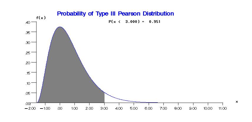
Figure 1: A type III Pearson distribution with a probability value indicated.

4 Evaluation of the program

To evaluate the accuracy of the SAS/IML macro program for computing and graphing probability values of Pearson distributions, the calculated parameters of the approximated Pearson distributions from this SAS/IML macro were first compared with the corresponding ones in Elderton and Johnson (1969). As can be seen in Table 2, the absolute differences between the calculated parameters from the SAS/IML macro and those from Elderton and Johnson (1969)’s tables are all very small with almost all of them less than .001 and a few less than .019. The same story applies to the relative differences with an unsurprising exception (4.46%) of $\kappa$ for type IV whose original magnitude is very small.

		Value from	Value from Elderton	Absolute	Relative
Typea	Parameter	SAS/IML Macro	and Johnson (1969)	Differenceb	Differencec
I	$\beta_{1}$	.507296	.507296	$<.0001$	$<.01$%
	$\beta_{2}$	2.935111	2.935110	$<.0001$	$<.01$%
	$\kappa$	-.264690	-.264500	.0002	.07%
	$r$	5.186821	5.186811	$<.0001$	$<.01$%
	$\alpha_{1}$	1.977543	1.996380	.0188	.94%
	$\alpha_{2}$	13.508428	13.527280	.0189	.14%
	$m_{1}$	.406954	.409833	.0029	.70%
	$m_{1}$	2.779867	2.776878	.0030	.12%
IV	$\beta_{1}$	.005366	.005366	$<.0001$	$<.01$%
	$\beta_{2}$	3.172912	3.172912	$<.0001$	$<.01$%
	$\kappa$	.012230	.012800	.0006	4.46%
	$r$	39.442562	39.442540	$<.0001$	$<.01$%
	$v$	4.388796	4.388794	$<.0001$	$<.01$%
	$\alpha$	13.111988	13.111980	$<.0001$	$<.01$%
	$m$	20.721280	20.721270	$<.0001$	$<.01$%
VI	$\beta_{1}$	.995360	.995361	$<.0001$	$<.01$%
	$\beta_{2}$	4.739349	4.739349	$<.0001$	$<.01$%
	$\kappa$	1.894437	1.895000	.0006	.03%
	$r$	-33.421430	-33.421290	.0001	$<.01$%
	$q_{1}$	42.030520	42.030800	.0003	$<.01$%
	$q_{2}$	6.609095	6.609500	.0004	$<.01$%
	$\alpha$	10.379832	10.379470	.0004	$<.01$%
aElderton and Johnson (1969) does not have the other types of Pearson distributions.
bAbsolute Difference = $\lvert$Value from Elderton and Johnson (1969) $-$ Value from SAS/IML Macro$\rvert$.
cRelative Difference = $\lvert$(Value from Elderton and Johnson (1969) $-$ Value from SAS/IML Macro)
		/Value from Elderton and Johnson (1969)$\rvert\times$100%.

Table 2: Computed parameters and their accuracy.

Then, the computed probability values from the SAS/IML macro were evaluated using the percentage points in Pearson and Hartley (1972)’s Table 32 (p. 276) corresponding to probability values of 2.5% and 97.5%. From Table 3, we can see that the probability values computed from the SAS/IML macro are very close to .025 (or 2.5%) and .975 (or 97.5%), respectively, with a high degree of precision (less than .0001).

			Percentage Point
			from Pearson and			Probability Value			Absolute
			Hartley (1972)			from SAS/IML Macro			Differenceb
Typea	$\surd{\beta_{1}}$	$\beta_{2}$	For 2.5%	For 97.5%		2.5%	97.5%		For 2.5%	For 97.5%
Normal	.0	3.0	-1.9600	1.9600		.0249970	.9750020		$<.00001$	$<.00001$
I	.6	3.2	-1.5998	2.2320		.0249965	.9749989		$<.00001$	$<.00001$
II	.0	2.6	-1.9196	1.9196		.0250030	.9749970		$<.00001$	$<.00001$
IV	1.4	8.6	-1.5068	2.3801		.0249838	.9749471		.00002	.00005
VI	2.0	11.2	-1.1915	2.5545		.0250054	.9750021		.00001	$<.00001$
VII	.0	8.4	-1.9925	1.9925		.0249999	.9750001		$<.00001$	$<.00001$
aPearson and Hartley (1972) does not have examples of types III and V.
bAbsolute Difference = $\lvert$.025 $-$ Probability value from SAS/IML macro$\rvert$, and = $\lvert$.975 $-$ Probability value
from SAS/IML macro$\rvert$, respectively.

Table 3: Computed probability values and their accuracy.

5 Concluding remarks

The new SAS/IML macro program provides an efficient and accurate means to compute probability values of Pearson distributions for which any data can be approximated based on the first four moments of the data. Thus, researchers can utilize this SAS/IML macro program in conducting distribution-free statistical analysis for any data with unknown distributions. The SAS/IML macro program also provides a nice feature of graphing the probability values of Pearson distributions to visualize the probability values on the Pearson distribution curves. For future study, it would be desirable to develop the similar program in other commonly used statistical language such as R or Stata.

Supplementary Material

The SAS/IML macro program for computing and graphing probability values of Pearson distributions is available as an ancillary file, PearsonDistributionProb.txt.

References

- Amos and Daniel (1971) Amos, D. E. and S. L. Daniel (1971). Tables of percentage points of standardized pearson distributions. Research Report SC-RR-71 0348, Sanida Laboratories, Albuquerque, NM.
- Bouver and Bargmann (1974) Bouver, H. and R. E. Bargmann (1974). Tables of the standardized percentage points of the pearson system of curves in terms of and . Technical Report No. 107, Department of Statistics and Computer Science, University of Georgia, Georgia, GA.
- Bowman and Shenton (1979) Bowman, K. O. and L. R. Shenton (1979). Approximate percentage points for pearson distributions. Biometrika 66(1), 147–151.
- Davis and Stephens (1983) Davis, C. S. and M. A. Stephens (1983). Approximate percentage points using pearson curves. Applied Statistics 32(3), 322–327.
- Elderton and Johnson (1969) Elderton, W. P. and N. L. Johnson (1969). Systems of Frequency Curves. Cambridge University Press, London.
- Pan (2009) Pan, W. (2009). A SAS/IML macro for computing percentage points of pearson distributions. Journal of Statistical Software 31(Code Snippet 2), 1–6.
- Pearson and Hartley (1972) Pearson, E. S. and H. O. Hartley (1972). Biometrika Tables for Statisticians, Volume II. Cambridge University Press, New York.
- Pearson (1895) Pearson, K. (1895). Contributions to the mathematical theory of evolution. ii. skew variations in homogeneous material. Philosophical Transactions of the Royal Society of London, Series A 186, 343–414.
- SAS Institute Inc. (2011) SAS Institute Inc. (2011). SAS/IML 9.3 User’s Guide. Cary, NC.
- Solomon and Stephens (1978) Solomon, H. and M. A. Stephens (1978). Approximations to density functions using pearson curves. Journal of the American Statistical Association 73(361), 153–160.