Localized analytical solutions and parameters analysis in the nonlinear dispersive Gross-Pitaevskii mean-field GP$(m,n)$ model with space-modulated nonlinearity and potential

Abstract

 

The novel nonlinear dispersive Gross-Pitaevskii (GP) mean-field model with the space-modulated nonlinearity and potential (called GP$(m,n)$ equation) is investigated in this paper. By using self-similar transformations and some powerful methods, we obtain some families of novel envelope compacton-like solutions spikon-like solutions to the GP$(n,n)\ (n>1)$ equation. These solutions possess abundant localized structures because of infinite choices of the self-similar function $X(x)$. In particular, we choose $X(x)$ as the Jacobi amplitude function ${\rm am}(x,k)$ and the combination of linear and trigonometric functions of space $x$ so that the novel localized structures of the GP$(2,2)$ equation are illustrated, which are much different from the usual compacton and spikon solutions reported. Moreover, it is shown that GP$(m,1)$ equation with linear dispersion also admits the compacton-like solutions for the case $0<m<1$ and spikon-like solutions for the case $m<0$.

 

1.  Introduction

Soliton plays a more and more important role and has many applications in the field of nonlinear science such as plasma physics, nonlinear optics, Bose-Einstein condensation, and finance, etc. The generation of soliton is due to the balance between (linear) dispersion and the nonlinear interaction soli . Since soliton was coined by Zabusky and Kruskal in 1965 Soliton , many new types of solitons have been reported such as optical solitons, breather solitons, dromion solutions, peakons, compactons, rogons, etc Op ; Op1 ; Op2 ; Op3 ; S2 ; yan10 ; R1 . It is still an interesting subject to investigate various of exact analytical solutions, in particular solitons, of nonlinear physical equations.

The compacton was first presented in the study of the KdV equation with nonlinear dispersion (called K$(m,n)$ equation) twenty years ago R1 ; R2 ; R22 , and it was shown that the K$(n,n)$ equation admitted a new kind of solitons, called compactons, which usually are described by powers of trigonometric functions in its one minimum period and exist in nonlinear wave equations with nonlinear dispersion. While compactons are the essence of the focusing branch, spikes, peaks and cusps are the hallmark of the defocusing branch which also supports the motion of kinks. The defocusing branch was found to give rise to solitary patterns having infinite slopes or cusps R1 -Yan62 . Up to now many different types of compactons were also presented, containing the discrete compactons D1 ; D2 ; D22 ; D3 ; D33 , breather compactons BC ; BC2 ; BC3 , elliptic compactons Yane , envelope compactons Yan6 ; Yan62 , etc. Moreover, it was found that nonlinear dispersion is not necessary condition to possess compactons and solitary patterns for nonlinear wave equation Yan ; Yan1 ; Yan6 ; Yan62 . Recently, we have presented the new nonlinear dispersive K$(m,n)$ model with variable coefficients and investigated its some solutinos Yank .

The one-dimensional Gross-Pitaevskii (GP) mean-field equation

$$i\hbar\frac{\partial}{\partial t}\psi=\left[-\frac{\hbar^{2}}{2M}\frac{\partial^{2}}{\partial x^{2}}+V_{\rm ext}(x)+g_{\rm 1D}|\psi|^{2}\right]\psi,$$ (1)

is a very important model to describe the static and dynamical properties of a Bose-Einstein condensation (BEC) BEC ; BEC2 ; BEC3 ; BEC4 , where $\psi\equiv\psi(x,t)$ is the condensate wavefunction, $M$ is the atmoic mass, $V_{\rm ext}(x)$ denotes the external potential and is usually chosen as the harmonic potential and optical lattice potential, $g_{\rm 1D}=2\hbar^{2}\omega_{\bot}a_{s}/M$ stands for the effective one-dimensional coupling strength with $\omega_{\bot}$ being the transverse confining frequency, and $a_{s}$ being the $s$-wave scattering length ($a_{s}>0\,(<0)$ corresponding to the repulsive (attractive) interaction), in which $a_{s}$ is a function of the magnetic field $B$ in the form fr1 ; fr2

$$a_{s}(B)=a_{0}\left(1-\frac{\Delta}{B-B_{0}}\right),$$

where $a_{0}$ denotes the background scattering length, which is the scattering length associated with the background potential, the parameter $B_{0}$ stands for the resonance position, and the parameter $\Delta$ is the resonance width.

Up to now, various types of the generalized GP equation with space- and time-modulated coefficients have been reported GP ; GP1 ; GP2 ; GP3 ; GP4 such as space- and time-modulated potential and nonlinearity, and the higher-degree nonlinearities. Recently, we introduced and studied the novel nonlinear Schrödinger equation with nonlinear dispersion $\partial_{x}^{2}(|\psi|^{n-1}\psi)$ and constant coefficients (called NLS$(m,n)$ equation) Yan6

$$i\frac{\partial\psi}{\partial t}=-\frac{\partial^{2}}{\partial x^{2}}(|\psi|^{n-1}\psi)+\gamma|\psi|^{m-1}\psi,\ \ (\gamma=\pm 1)$$ (2)

and two generalized higher-order nonlinear Schrödinger equations with nonlinear dispersion and constant coefficients (called GNLS$(m,n)$ equations) Yan62

$$i\frac{\partial\psi}{\partial t}+a\frac{\partial^{2}}{\partial x^{2}}(|\psi|^{n-1}\psi)+b|\psi|^{m-1}\psi+ic\frac{\partial^{3}}{\partial x^{3}}(|\psi|^{p-1}\psi)+id\frac{\partial}{\partial x}(|\psi|^{q-1}\psi)=0,$$ (3)

$$i\frac{\partial\psi}{\partial t}+a\frac{\partial^{2}}{\partial x^{2}}(|\psi|^{n-1}\psi)+b|\psi|^{m-1}\psi+ic\frac{\partial^{3}}{\partial x^{3}}(|\psi|^{p-1}\psi)+ih|\psi|^{q-1}\frac{\partial}{\partial x}\psi=0,$$ (4)

and obtained their some types of envelope compactons and spikons for some different parameters $m,\,n,\,p,\,q$  Yan6 ; Yan62 , where $m,\,n,\,p,\,q,\,a,\,b,\,c,\,d,\,$ and $h$ are real-valued constants. To our knowledge, compacton-like and spikon-like solutions of nonlinear complex dispersive wave equations with varying coefficients were not reported before.

In this paper, we extended the ideas Yank ; Yan6 ; Yan62 to the GP equation and introduce the nonlinear dispersive GP equation with space-modulated potential and nonlinearity (called GP$(m,n)$ equation) such that novel localized solutions are found. These solution profiles are very different from the usual compacton and spikon solutions. The rest of this paper is organized as follows. In Section 2, we introduce the nonlinear dispersive GP model with varying coefficients, which is called the GP$(n,n)$ equation. In Section 3, we obtained self-similar solutions including compacton-like and spikon-like solutions of GP$(n,n)$ and GP$(m,1)$ equations. We analyze the localized solutions for the chosen function $X(x)$ to be the Jacobi amplitude function ${\rm am}(x,k)$ and the combination of linear and trigonometric functions of $x$ in Section 4. Finally, some conclusions are given in last section.

2.  Nonlinear dispersive GP model with space-modulated potential

and nonlinearity: GP$(m,n)$ equation

To understand the role of nonlinear dispersion in the one-dimensional dimensionless GP mean-field model arising from Bose-Einstein condensates, we introduce and study the dimensionless nonlinear dispersion GP equation by replacing the linear dispersion $\partial_{x}^{2}\psi$ with nonlinear dispersion $\partial_{x}^{2}(|\psi|^{n-1}\psi)$ and changing the nonlinear term, described by

$$i\frac{\partial\psi}{\partial t}=-\frac{\partial^{2}}{\partial x^{2}}(|\psi|^{n-1}\psi)+v(x)\psi+g(x)|\psi|^{m-1}\psi,\qquad(n\geq 1)$$ (5)

which is simply referred to as the GP$(m,n)$ equation, where $\psi=\psi(x,t)$ is a complex field, $m$ and $n$ are real-valued parameters, $v(x)$ is a linear (trap) potential, and $g(x)$ describes the spatial modulation of the nonlinearity. GP$(m,n)$ equation (5) contains many types of nonlinear wave equations. If $v(x)\equiv 0$ and $g(x)$ is a constant, then Eq. (5) becomes the NLS$(m,n)$ equation (4). Though Eq. (5) is in fact the generalized GP equation with the linear dispersion for the case $n=1$, but we will investigate its new wave structures such as compacton and spikon solutions not solitary wave structures. In particular, i) for the case $n=1$ and $m=3$, the GP$(3,1)$ equation reduces to the usual GP equation with space-modulated coefficients

$$i\frac{\partial\psi}{\partial t}=-\frac{\partial^{2}\psi}{\partial x^{2}}+v(x)\psi+g(x)|\psi|^{2}\psi,$$ (6)

whose periodic wave solutions and solitary wave solutions were obtained for different potentials and nonlinrarities GP ; GP1 ; GP2 ; GP3 ; GP4 ; ii) for the case $n=1$ and $m>1$, the GP$(m,1)$ equation becomes the generalized GP model GPg

$$i\frac{\partial\psi}{\partial t}=-\frac{\partial^{2}\psi}{\partial x^{2}}+v(x)\psi+g(x)|\psi|^{m-1}\psi,$$ (7)

iii) for the case $n=m=1$, the GP$(1,1)$ equation becomes the linear GP (NLS) model with the potential $v(x)+g(x)$:

$$i\frac{\partial\psi}{\partial t}=-\frac{\partial^{2}\psi}{\partial x^{2}}+[v(x)+g(x)]\psi.$$ (8)

In what follows, we will focus on compacton-like solutions and spikon-like solutions of GP$(m,n)$ equation except for the above-mentioned three cases by using self-similar transformations and some ansatze.

3.  General theory and self-similar solutions

In general, Eq. (5) is not integrable for the case $n\not=1,\,m\not=2$. It is difficult to solve directly Eq. (5). We need reduce Eq. (5) to some equations solving easily. Eq. (5) may possess many types of similarity reductions by using the symmetry analysis (see, e.g., lie ; lie2 ). Our goal is to reduce the solutions of GP$(m,n)$ equation (5) to those of the stationary Gross-Pitaevskii equation with nonlinear dispersion (called SGP$(m,n)$ equation)

$$\mu\Phi(X)=-\frac{d^{2}\Phi^{n}(X)}{dX^{2}}+G\Phi^{m}(X),$$ (9)

where $\Phi(X)$ is the real-valued stationary field, $X\equiv X(x)$ is an unknown function of space $x$ to be determined, $\mu$ is the real eigenvalue of the nonlinear wave equation (9), and $G$ is a real coefficient of the nonlinearity. Eq. (9) is a complicated nonlinear ordinary differential equation. When $n=1,\,m=3$, Eq. (9) is the stationary nonlinear Schrödinger equation or stationary Gross-Pitaevskii equation without a potential $\mu\Phi(X)=-\frac{d^{2}\Phi(X)}{dX^{2}}+G\Phi^{3}(X)$, which admits the bright ($G<0$) and dark ($G>0$) solitary wave solutions GP3 . We explore the following self-similar transformation (the stationary solutions)

$$\psi(x,t)=\rho(x)e^{i\varphi(t)}\Phi[X(x)],$$ (10)

to the GP$(m,n)$ equation (5) such that we have the nonlinear differential equation:

$$\begin{array}[]{l}\varphi_{t}(t)\rho(x)\Phi(X)-n\rho^{n}(x)X_{x}^{2}\Phi^{n-1}(X)\Phi_{XX}(X)-n(n-1)\rho^{n}(x)X_{x}^{2}\Phi^{n-2}(X)\Phi_{X}^{2}(X)\vspace{0.15in}\cr\quad-n\rho^{n-1}(x)\rho_{xx}(x)\Phi^{n}(X)-2n^{2}\rho^{n-1}(x)\rho_{x}(x)X_{x}\Phi^{n-1}(X)\Phi_{X}(X)-n\rho^{n}(x)X_{xx}\Phi^{n-1}(X)\Phi_{X}(X)\vspace{0.15in}\cr\quad-n(n-1)\rho^{n-2}(x)\rho_{x}^{2}(x)\Phi^{n}(X)+v(x)\rho(x)\Phi(X)+g(x)\rho^{m}(x)\Phi^{m}(X)=0,\end{array}$$ (14)

where the subscripts denote the partial derivative with respect to the related variables, $\rho(x)$ denotes the amplitude of the wave function, and $\varphi(t)$ is the phase,

It follows from Eq. (14) that all other terms are functions of space $x$ except for the term $\varphi_{t}(t)\rho(x)\Phi(X)$. Thus we require that the function $\varphi_{t}(t)$ should be a non-zero constant (e.g, $\varphi_{t}=\omega={\rm const}$). Since we require that $\Phi(X)$ satisfies Eq. (9), thus we balance the coefficients of the related terms to obtain the following two possible systems in these unknown functions $\rho(x),\ g(x),\ v(x)$, and $\varphi(t)$ for different types of parameters $m$ and $n$:

System I :  for the case $n=m$.

$$\begin{array}[]{l}\varphi_{t}(t)=\omega,\vspace{0.1in}\cr[\rho^{2n}(x)X_{x}]_{x}=0,\vspace{0.1in}\cr v(x)=-\mu\rho^{n-1}(x)X_{x}^{2}-\omega,\vspace{0.1in}\cr g(x)=\displaystyle\frac{[\rho^{n}(x)]_{xx}}{\rho^{n}(x)}+GX_{x}^{2},\end{array}$$ (19)

System II :  for the case $n=1$.

$$\begin{array}[]{l}\varphi_{t}(t)=\omega,\vspace{0.1in}\cr[\rho^{2}(x)X_{x}]_{x}=0,\vspace{0.1in}\cr v(x)=\displaystyle\frac{\rho_{xx}(x)}{\rho(x)}-\mu X_{x}^{2}-\omega,\vspace{0.1in}\cr g(x)=G\rho^{1-m}(x)X_{x}^{2},\end{array}\qquad\ \$$ (24)

where $\omega$ is the chemical potential.

The compacton solutions and spikon solutions of the SGP$(m,n)$ equation (9) are listed in Table I for differential parameters $G,\ \mu,\ m$ and $n$ by using the direct cosine and sinh-cosh transformations R1 ; R2 ; Yan ; Yan1 ; Yan6 ; Yan62 , in which the first three solutions are compacton solutions and other ones are spikon solutions of SGP$(m,n)$ equation. For the first three compacton solutions in Table I, we require that $|\nu X|\leq\pi/2$, and $\Phi(X)$ vanishes elsewhere. We can determine, after some straightforward algebra, the corresponding functions, necessary for GP$(m,n)$ equation (5) to admit analytical envelope compacton-like solutions and spikon-like solutions in terms of the self-similar transformation (10).

If we choose $X=X(x)$ as a free function, then one can find that the nonlinearity $g(x)$ and external potential $v(x)$ depend only on $X(x)$ and two sets of exact solutions of system (I) and (II) are listed below:

Solution I :  for the case $n=m.$

$$\begin{array}[]{l}\varphi(t)=\omega t,\vspace{0.1in}\cr\rho(x)=\displaystyle\left(CX_{x}\right)^{-\frac{1}{2n}},\vspace{0.1in}\cr g(x)=\displaystyle\sqrt{CX_{x}}\left(\frac{1}{\sqrt{CX_{x}}}\right)_{xx}+GX_{x}^{2},\vspace{0.1in}\cr v(x)=\displaystyle-\mu X_{x}^{2}\left(CX_{x}\right)^{\frac{1-n}{2n}}-\omega,\end{array}$$ (29)

Solution II :  for the case $n=1.$

$$\begin{array}[]{l}\varphi(t)=\omega t,\vspace{0.1in}\cr\rho(x)=\displaystyle\left(CX_{x}\right)^{-\frac{1}{2}},\vspace{0.1in}\cr g(x)=\displaystyle GX_{x}^{2}\left(CX_{x}\right)^{\frac{m-1}{2}},\vspace{0.1in}\cr v(x)=\displaystyle\sqrt{CX_{x}}\left(\frac{1}{\sqrt{CX_{x}}}\right)_{xx}-\mu X_{x}^{2}-\omega,\end{array}$$ (34)

where $C\not=0$ is an integration constant, and $CX_{x}>0$.

Therefore, in terms of transformation (10), we obtain the following two families of novel analytical solutions with an arbitrary function $X(x)$ of the GP$(m,n)$ equation (5)

$$\psi_{1}(x,t)=\frac{e^{i\omega t}}{\sqrt[2n]{CX_{x}}}\Phi[X(x)],\ \ {\rm for}\ \ n=m>1,$$ (35)

$$\psi_{2}(x,t)=\frac{e^{i\omega t}}{\sqrt{CX_{x}}}\Phi[X(x)],\ \ {\rm for}\ \ n=1,\ m<1,$$ (36)

where the solutions $\Phi(X(x))$ of the SGP$(m,n)$ equation (9) with the different parameters are given in Table I, in which we require that $\mu>0$ for cases $2$ and $3$ and $\mu<0$ for cases $4,\,5,\,8,$ and $9$.

TABLE I.  Solutions of the SGP$(m,n)$ equation (9)
Case $G$
  $A$   $\nu$  $(n,\,m)$   $\Phi(X)$ 1 $-1$ $\ \ \displaystyle-\frac{2n\mu}{n+1}$ $\ \ \displaystyle\frac{n-1}{2n}$ $n=m>1$ $[A\cos^{2}(\nu X)]^{\frac{1}{n-1}}$ 2 $-1$ $\displaystyle-\frac{\mu(m+1)}{2}$ $\displaystyle\frac{\sqrt{\mu}\,(1-m)}{2}$ $n=1$ $[A\cos^{2}(\nu X)]^{\frac{1}{1-m}}$ 3 $\ \ 1$ $\ \ \displaystyle\frac{\mu(m+1)}{2}$ $\displaystyle\frac{\sqrt{\mu}\,(1-m)}{2}$ $n=1$ $[A\cos^{2}(\nu X)]^{\frac{1}{1-m}}$ 4 $-1$ $\ \ \displaystyle\frac{\mu(m+1)}{2}$ $\displaystyle\frac{\sqrt{-\mu}\,(1-m)}{2}$ $n=1,\,m<1$ $[A\sinh^{2}(\nu X)]^{\frac{1}{1-m}}$ 5 $-1$ $\displaystyle-\frac{\mu(m+1)}{2}$ $\displaystyle\frac{\sqrt{-\mu}\,(1-m)}{2}$ $n=1,\,m<1$ $[A\cosh^{2}(\nu X)]^{\frac{1}{1-m}}$ 6 $\ \ 1$ $\ \ \displaystyle-\frac{2n\mu}{n+1}$ $\ \ \displaystyle\frac{n-1}{2n}$ $n=m>1$ $[A\sinh^{2}(\nu X)]^{\frac{1}{n-1}}$ 7 $\ \ 1$ $\ \ \ \ \displaystyle\frac{2n\mu}{n+1}$ $\ \ \displaystyle\frac{n-1}{2n}$ $n=m>1$ $[A\cosh^{2}(\nu X)]^{\frac{1}{n-1}}$ 8 $\ \ 1$ $\displaystyle-\frac{\mu(m+1)}{2}$ $\displaystyle\frac{\sqrt{-\mu}\,(1-m)}{2}$ $n=1,\,m<1$ $[A\sinh^{2}(\nu X)]^{\frac{1}{1-m}}$ 9 $\ \ 1$ $\ \ \displaystyle\frac{\mu(m+1)}{2}$ $\displaystyle\frac{\sqrt{-\mu}\,(1-m)}{2}$ $n=1,\,m<1$ $[A\cosh^{2}(\nu X)]^{\frac{1}{1-m}}$

Without loss of generality, we choose the condition $CX_{x}>0$ in Eqs. (29)-(36) as

$$C=1,\qquad X_{x}>0.$$ (37)

The self-similar variable $X(x)$ admits an infinite choices such that the corresponding exact solutions of GP$(m,n)$ equation (5) will display the abundant structures. For the simple case $X(x)=ax+b$ ($a>0$ since $X_{x}>0$ is required), it follows from Eqs. (29)-(36) that all these functions $\rho(x),\ g(x)$ and $v(x)$ reduce to the constants and the obtained exact solutions (35) and (36) become the analytical travelling wave solutions which illustrate envelope compacton solutions and spikon solutions of GP$(m,n)$ equation (5) with constant coefficients Yan6 . Here we do not consider the travelling wave case, i.e, $X(x)=ax+b$ ($a>0$ since $X_{x}>0$ is required).

4.  Wave propagations of envelope solutions

4.1  Attractive nonlinearity $G<0$

In this case we take $G=-1$. In the following we will choose some functions for the variable $X(x)$ to study the wave propagations of the solutions (35) and (36) of Eq. (5).

Choice I of $X(x)$.  To consider the envelope compacton-like solutions of the GP$(2,2)$ equation (5) is given by Eq. (35) with $\Phi(X)$ defined by Case 1 in Table I. We here focus on $X=X(x)$ as the Jacobi amplitude function

$$X(x)=2\ {\rm am}(x,k),\ \ \ {\rm for\ \ all}\ \ x\in\mathbb{R}$$ (38)

which satisfies the required condition $X_{x}=2\,{\rm dn}(x,k)>0$, where ${\rm am}(x,k)$ is the elliptic integrals of the Jaocibi elliptic function ${\rm dn}(x,k)$ with the modulus $k\in(0,1)$ DN , i.e.

$${\rm am}(x,k)=\int^{x}_{x_{0}}{\rm dn}(s,k)ds,\qquad|{\rm am}(x,k)|\leq\pi.$$

Thus we have $|X(x)|\leq 2\pi$ in terms of Eq. (38), which just leads to the required region of the independent variable $|\nu X(x)|$ of $\Phi(X)$, i.e.,

$$|\nu X(x)|=\left|\frac{1}{4}X(x)\right|=\left|\frac{1}{2}\,{\rm am}(x,k)\right|\leq\frac{\pi}{2},\ \ {\rm for\ \ all}\ \ x\in\mathbb{R}$$ (39)

Moreover, for the $X(x)$ defined by Eq. (38), the nonlinearity $g(x)$ and external potential $v(x)$ of the GP$(n,n)$ equation are rewritten as

$$\begin{array}[]{l}v(x)=-\mu[2\ {\rm dn}(x,k)]^{7/4}-\omega,\vspace{0.1in}\cr g(x)=\displaystyle-\frac{1}{4}\Big{[}15\,{\rm dn}^{2}(x,k)+3(1-k^{2})\,{\rm nd}^{2}(x,k)+k^{2}-2\Big{]},\end{array}$$ (42)

where ${\rm nd}(x,k)=1/{\rm dn}(x,k)$.

We require that the compacton solution $\Phi(X)$ of the SGP$(n,n)$ equation (9) is non-zero ($[A\cos^{2}(\nu X)]^{\frac{1}{n-1}}\not=0$) only in its one period $(|\nu X|\leq\pi/2)$ nearby the origin and zero for all other region for $X$, but the intensity $|\psi_{1}(x,t)|^{2}$ related to the corresponding solution (35) of GP$(n,n)$ is only a function of $x$. It follow from Eqs. (38) and (39) that the compacton-like solution of the GP$(n,n)$ equation is nontrivial for all $x\in\mathbb{R}$, which is very different from properties of the usual compacton solutions R1 , because of the choice of $X(x)$, which is related to the potential $v(x)$ and nonlinearity $g(x)$ (see Eq. (29)).

To illustrate the effect of $X(x)$ in the compacton-like solution (35), The compacton solution of the SGP$(n,n)$ equation (9) given in Case 1 of Table I is displayed in Fig. 1(a) with respect to the variable $X$ not $x$. The corresponding envelope compacton solutions of GP$(n,n)$ equation (5) is a non-travelling wave solution for $x$

$$\psi(x,t)=\frac{1}{\sqrt[2n]{2\,{\rm dn}(x,k)}}\left\{-\frac{2n\mu}{n+1}\cos^{2}\left[\frac{n-1}{n}\,{\rm am}(x,k)\right]^{1/(n-1)}\right\}e^{i\omega t},$$ (43)

and the intensity $|\psi(x,t)|^{2}$ is illustrated in Fig. 1(b) with respect to $x$. It is easy to see that the top part of the profile has so much changes when the modulus $k$ closes to $1$, which is different from the usual compacton solution illustrated in Fig. 1(a), since $X(x)$ is the Jacobi amplitude function of $x$ given by Eq. (38).

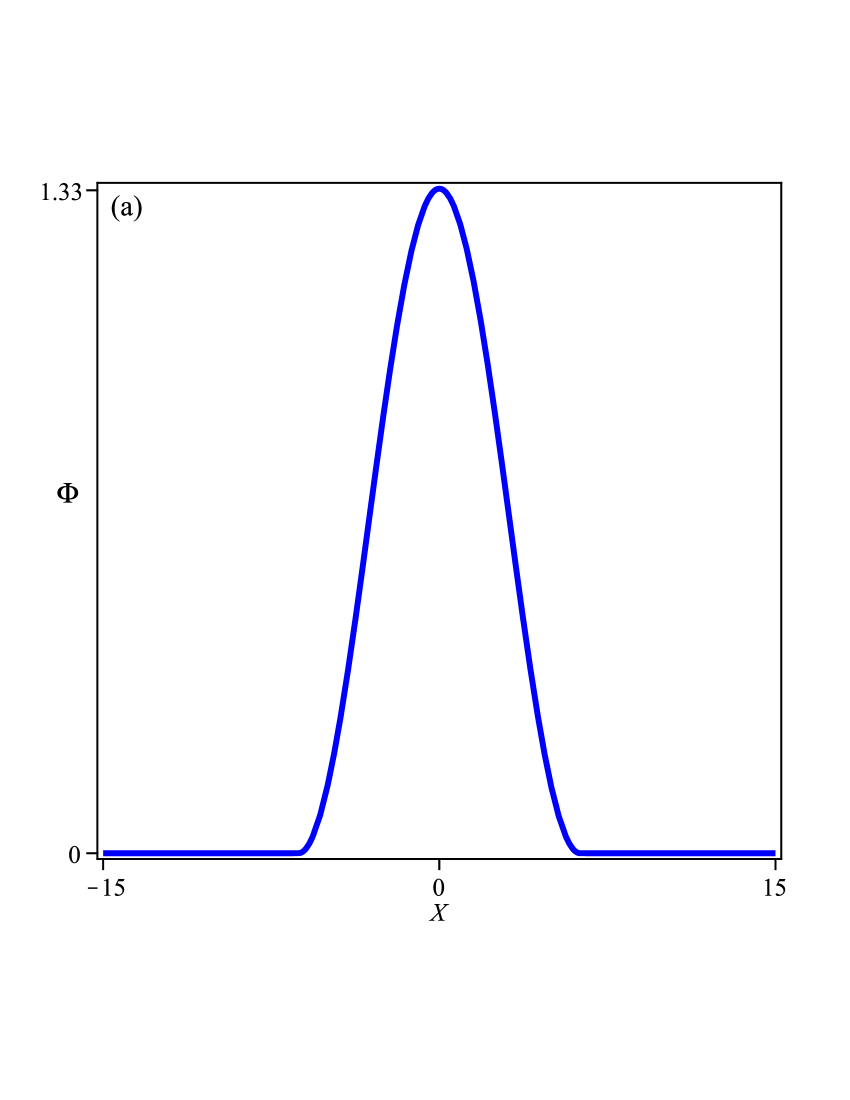
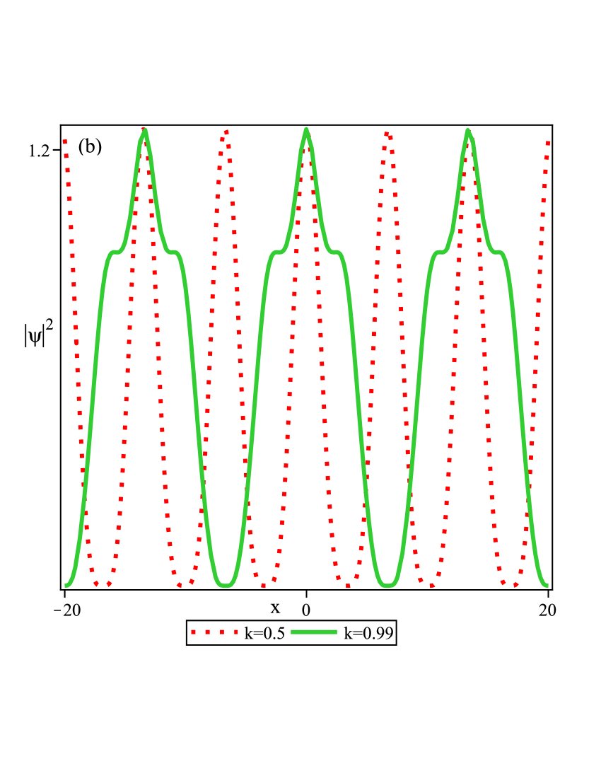
Figure 1: Plots of $\Phi(X)$ and $|\psi|^{2}$ with the parameters are $n=2,\ \mu=-1$. (a) $\Phi(X)$ given by Case 1 in Table I, (b) $|\psi(x,t)|^{2}$ given by Eq. (43) with $k=0.5$ and $k=0.99$.

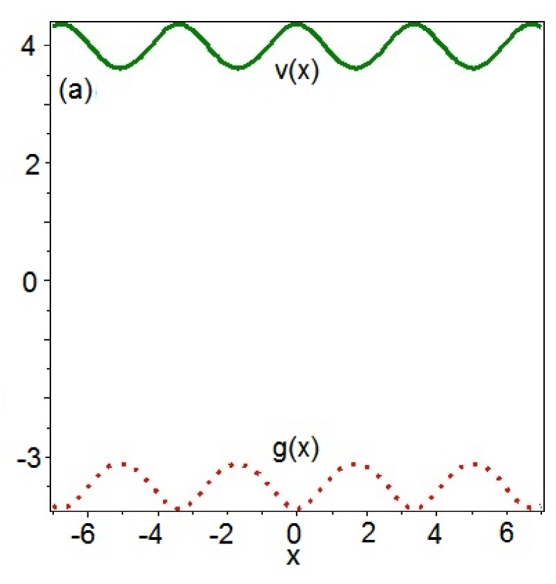
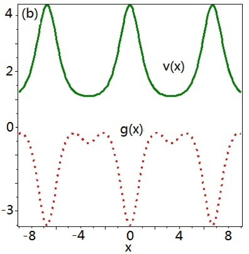
Figure 2: Plots of $g(x)$ and $v(x)$ given by Eq. (42) with $\omega=-1$ and othere parameters being the same as Figure 1. (a) $k=0.5$, (b) $k=0.99$.

In addition, the corresponding nonlinearity $g(x)$ and the external potential $v(x)$ given by Eq. (42) are also localized periodic waves and illustrated in Figs. 2(a,b). Of course we can also choose other functions about $X(x)$ to illustrate more types of solution structures.

For another case $n=1$ and $m<1$, in which GP$(m,1)$ becomes the linear dispersive GP equation. Without loss of generality, we choose $m=1/3,\ \mu=1$ and consider the exact solution (36) of $GP(1/3,1)$ equation with $\Phi(X)$ given by Case 2 in Table I. We still choose the similarity variable $X(x)$ as the Jacobi amplitude function in the form

$$X(x)=\frac{3}{2}\ {\rm am}(x,k),\ \ \ {\rm for\ \ all}\ \ x\in\mathbb{R}$$ (44)

which make sure that the following condition of the compacton solutions of SGP$(1/3,1)$ equation

$$|\nu X(x)|=\left|\frac{1}{3}X(x)\right|=\left|\frac{1}{2}\,{\rm am}(x,k)\right|\leq\frac{\pi}{2},\ \ {\rm for\ \ all}\ \ x\in\mathbb{R}$$ (45)

holds. Moreover, for the $X(x)$ defined by Eq. (38), the nonlinearity $g(x)$ and external potential $v(x)$ of the GP$(n,n)$ equation are rewritten as

$$\begin{array}[]{l}v(x)=\displaystyle\frac{1}{4}\Big{[}(1-9\mu)\,{\rm dn}^{2}(x,k)+3(k^{2}-1)\,{\rm nd}^{2}(x,k)-k^{2}+2\Big{]}-\omega,\vspace{0.1in}\cr g(x)=\displaystyle-\left[\frac{3}{2}\,{\rm dn}(x,k)\right]^{5/3},\end{array}$$ (48)

where ${\rm nd}(x,k)=1/{\rm dn}(x,k)$.

In Fig. 3(a), we display the plots of the intensity $|\psi(x,t)|^{2}$ of the solution given by Eq. (36) of GP$(m,1)$ equation in the form

$$\psi(x,t)=\frac{\sqrt{2/3}}{\sqrt{{\rm dn}(x,k)}}\left\{-\frac{\mu(m+1)}{2}\cos^{2}\left[\frac{3\sqrt{\mu}(1-m)}{4}\,{\rm am}(x,k)\right]^{3/2}\right\}e^{i\omega t},\,\,(m<1)$$ (49)

for different modulus $k=0.5$ and $k=0.99$. When $k$ closes to $1$ from $0.98$, the top part of the intensity profile appears the strong oscillation and there exist more branches. Thus it follows from the conclusions mentioned-above that the linear dispersive GP equation (GP$(m,1)$ equation) also admits the compacton-like solutions. Fig. 3(a) displays the profiles of the external potential and nonlinearity given by Eq. (48).

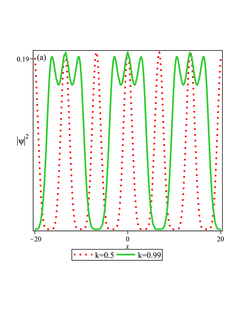
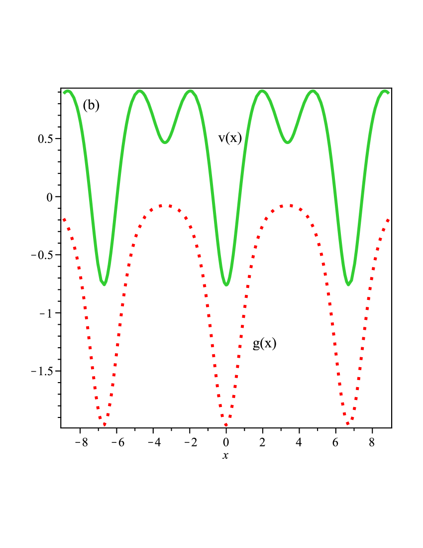
Figure 3: Solution (36) with $\Phi$ given in Case 2 of Table I with $X$ given by Eq. (44) for $m=1/3,\ \mu=1$. (a) Plot of $|\psi|^{2}$ given by Eq. (49) for $k=0.5,\ 0.99$, (b) Plots of $g(x)$ and $v(x)$ given by Eq. (48) with $k=0.99$.

Choice II of $X(x)$.  Here we consider another choice of $X(x)$ in the form of the combination of linear and trigonometric functions of $x$

$$X(x)=\alpha x+\sin(Kx),$$ (50)

where $\alpha>K>0$ leads to the condition $X_{x}=\alpha+K\cos(Kx)>0$. For the compacton-like solutions of the GP$(2,2)$ equation (5) is given by Eq. (35) with $\Phi(X)$ defined by Case 1 in Table I, we require that $x$ satisfies the condition ($n=m=2$)

$$|\nu X(x)|=\left|\frac{1}{4}X(x)\right|=\left|\frac{1}{4}[\alpha x+\sin(Kx)]\right|\leq\frac{\pi}{2},$$ (51)

For the given parameters $\alpha$ and $K$, one can find the region of $x$ which is a very small part of $(-\infty,\infty)$, distinguishing from the condition (39). The corresponding envelope compacton solutions of GP$(n,n)$ equation (5) is a non-travelling wave solution for $x$

$$\psi(x,t)=\frac{1}{\sqrt[2n]{\alpha+K\cos(Kx)}}\left\{-\frac{2n\mu}{n+1}\cos^{2}\left[\frac{n-1}{2n}\,(\alpha x+\sin(Kx))\right]^{1/(n-1)}\right\}e^{i\omega t},$$ (52)

In Fig. 4, we find that more strongly nonlinear wave oscillates, smaller the value $\beta=\alpha/K-1$ becomes. When $\beta=0.05$, the wave profile is divided into three parts being of three vertexes. Moveover, when $\beta$ closes to $0$, the middle vertex increases slowly, but the beside vertexes grow quickly. This is different from the usual compacton solutions (see Fig. 1(a)).

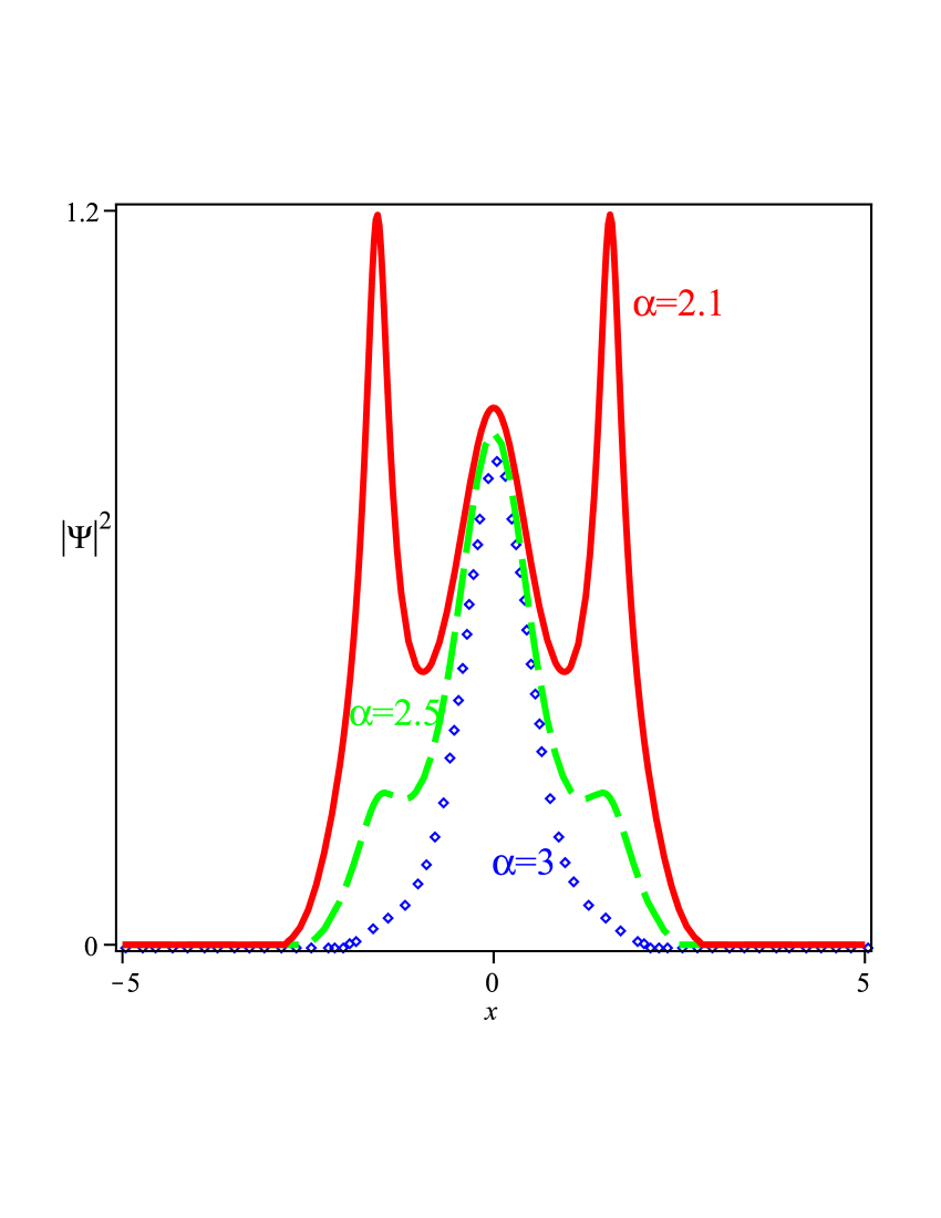
Figure 4: Plots of $|\psi(x,t)|^{2}$ given by Eq. (52) with the parameters $n=2,\ \mu=-1,\ K=2$ and $\alpha=3,\ 2.5,\ 2.1$.

In addition, based on Eqs. (29) and (50), we have the corresponding nonlinearity and potential in the form

$$\begin{array}[]{l}v(x)=-\mu[\alpha+K\cos(Kx)]^{7/4}-\omega,\vspace{0.1in}\cr g(x)=\displaystyle\frac{3K^{4}\sin^{2}(Kx)}{4\left[\alpha+K\cos\left(Kx\right)\right]^{2}}+\frac{K^{3}\cos\left(Kx\right)}{2\left[\alpha+K\cos(Kx)\right]}-[\alpha+K\cos(Kx)]^{2},\end{array}$$ (55)

which are illustrated in Figs. 5(a,b) for $\alpha=2.5,\,2.1$, and $K=2$.

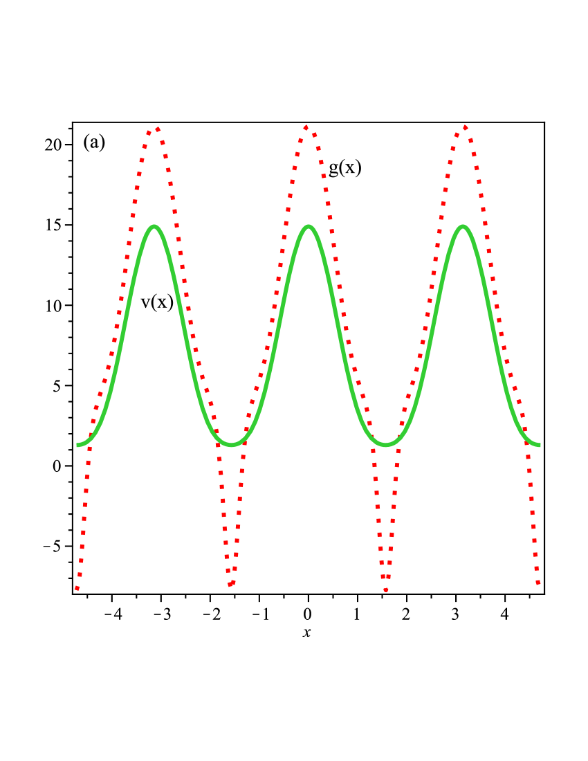
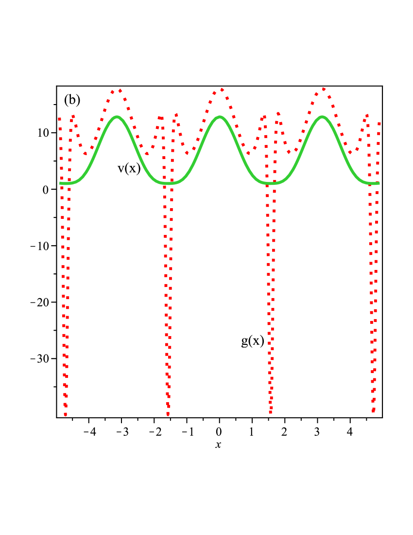
Figure 5: Plots of $g(x)$ and $v(x)$ given by Eq. (50) with $\omega=-1,\,\mu=-1,\,K=2$. (a) $\alpha=2.5$, (b) $\alpha=2.1$.

For the case $n=1,\ 0<m<1$, where we consider the analytical exact solution (36) of GP$(1/3,1)$ equation with $\Phi(X)$ given by Case 2 in Table I. We still choose the similarity variable $X(x)$ as (50) and we require that $x$ satisfies the condition

$$|\nu X(x)|=\left|\frac{1}{3}X(x)\right|=\left|\frac{1}{3}[\alpha x+\sin(Kx)]\right|\leq\frac{\pi}{2},$$ (56)

As a result, we have the envelope compacton-like solutions of GP$(m,1)$ equation in the form

$$\psi(x,t)=\frac{1}{\sqrt{\alpha+K\cos(Kx)}}\left\{-\frac{\mu(m+1)}{2}\cos^{2}\left[\frac{\sqrt{\mu}(1-m)}{2}\,[\alpha x+\sin(Kx)]\right]^{3/2}\right\}e^{i\omega t},\,\,(m<1)$$ (57)

In Fig. 6, we display the profile of the compacton-like solutions of GP$(m,1)$ equation and find that more strongly nonlinear wave oscillates, smaller the value $\beta=\alpha/K-1$ becomes. When $\beta=0.04$, the wave profile is divided into three parts being of three vertexes. Moveover, when $\beta$ closes to $0$, the middle vertex increases quickly, but the beside vertexes grow slowly. This is also different from the usual compacton solution.

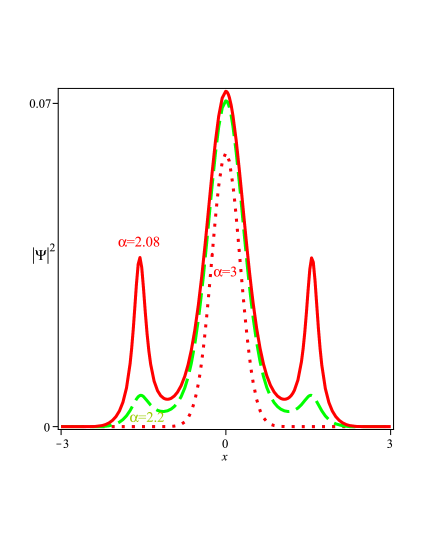
Figure 6: Plots of $|\psi(x,t)|^{2}$ given by Eq. (57), corresponding to $n=1,\ m=1/3,\ \mu=1,\ K=2$ and $\alpha=3,\ 2.2,\ 2.08$.

4.2  Repulsive nonlinearity $G>0$

In this case we take $G=1$, the envelope spikon-like solutions of the GP$(2,2)$ equation (5) is given by (35) with $\Phi(X)$ defined by Case 7 of Table I. We still choose $X$ as the form (38) even if we do not require the similar condition (39). Though the hyperbolic cosh function $\cosh(X)$ is infinite for $X$ approaches to infinity, we know that

$$|X(x)|\leq 2\pi\ \ {\rm and}\ \ X_{x}=2\ {\rm dn}(x,k)\in(0,\,2)\ \ {\rm for\ \ all}\ \ x\in\mathbb{R}.$$ (58)

Thus the novel spikon-like solution of GP$(n,n)$ equation is localized for all $x$ which is different from the usual spikon solutions R2 ; Yan ; Yan6 . Figure 7(a) denotes that the sipkon solution of SGP$(2,2)$ equation is not localized for the variable $X$, but the spikon-like solution of GP$(2,2)$ is localized because of the proper choice of $X(x)$ which is illustrated in Figure 7(b). Similarly, if we choose $\Phi(X)$ as the Case 6 in Table I, then the results are displayed in Figure 8.

For the case $n=1$ and $m<1$, without loss of generality, we choose $m=1/3,\ \mu=-1$ and consider the solution (36) of GP$(1/3,1)$ equation with $\Phi(X)$ given by Case 9 in Table I. We choose the new variable $X(x)$ as the Jacobi amplitude function (44). The profiles of intensity $|\psi(x,t)|^{2}$ are illustrated in Figures 9(a,b).

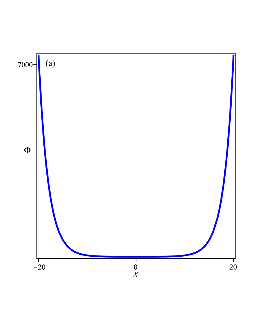
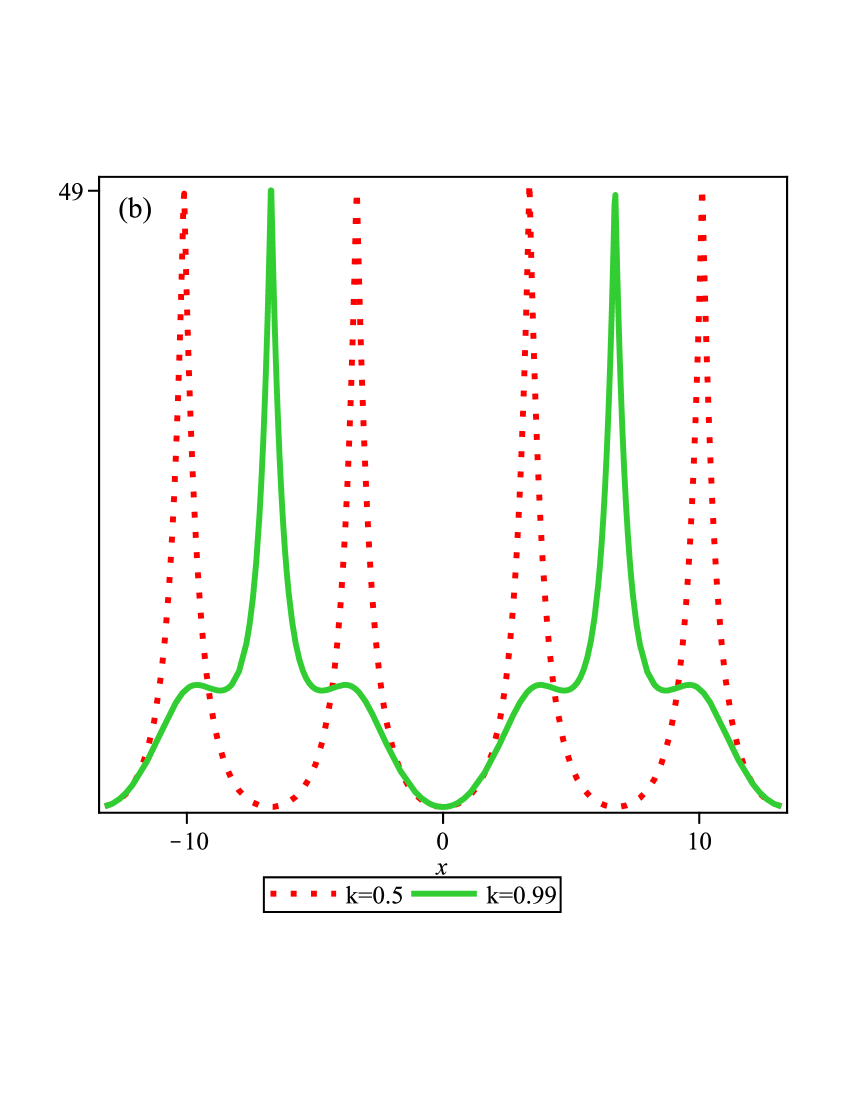
Figure 7: Solution given by Eq. (35) with $X(x)$ given by Eq. (38) and $\Phi(X)$ given by Case 7 in Table I, corresponding to (a) Plot of $\Phi(X)$ with $n=2,\ \mu=1$, (b) Plots of $|\psi|^{2}$ with $k=0.5$ and $k=0.99$.

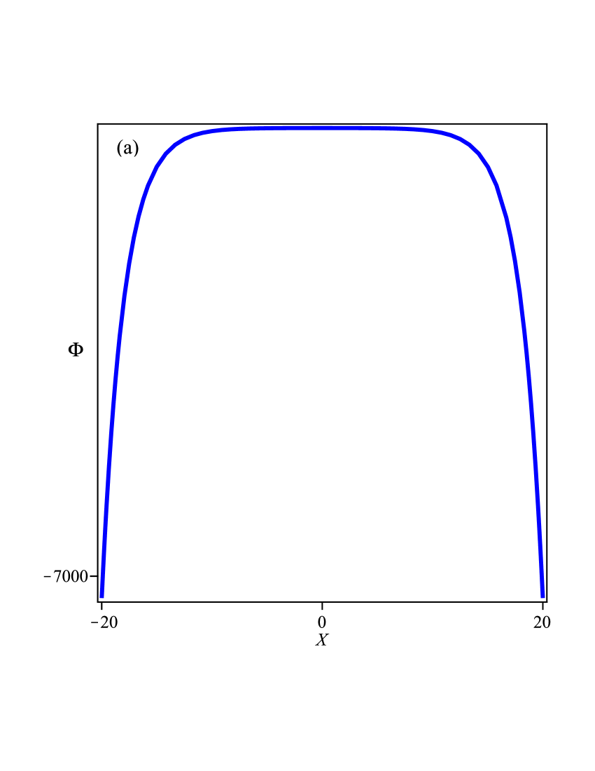
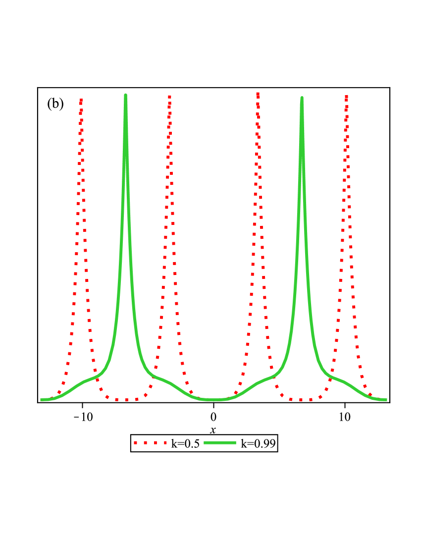
Figure 8: Solution given by Eq. (35) with $X(x)$ given by Eq. (38) and $\Phi(X)$ given by Case 6 in Table I, corresponding to (a) Plot of $\Phi(X)$ with $n=2,\ \mu=1$, (b) Plots of $|\psi|^{2}$ with $k=0.5$ and $k=0.99$.

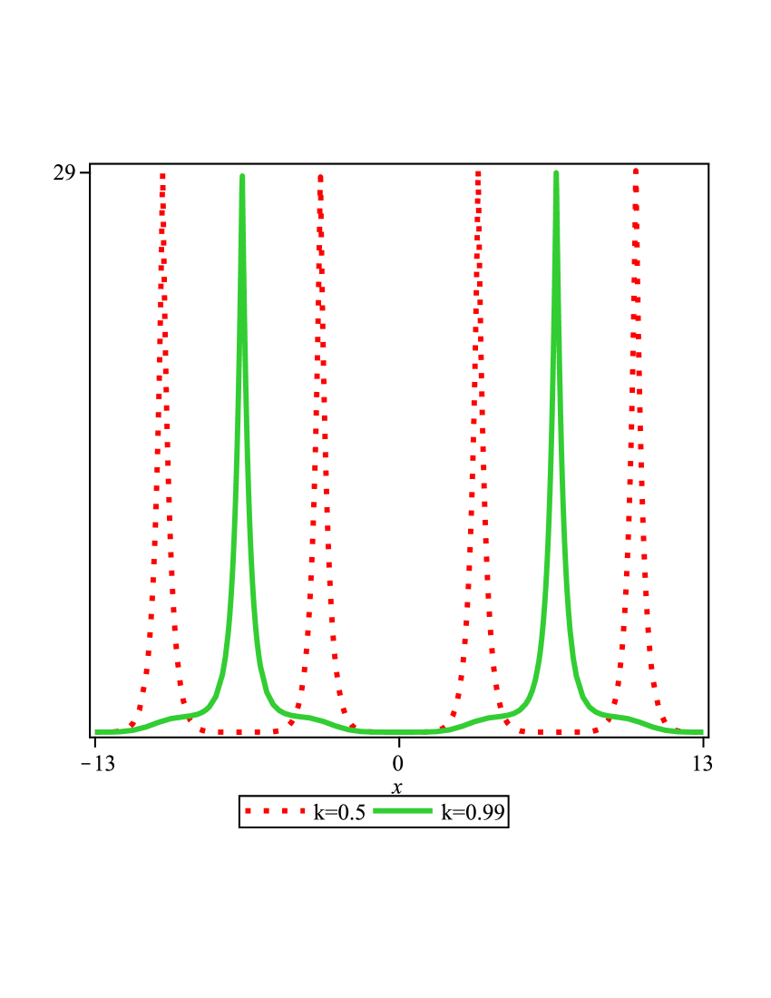
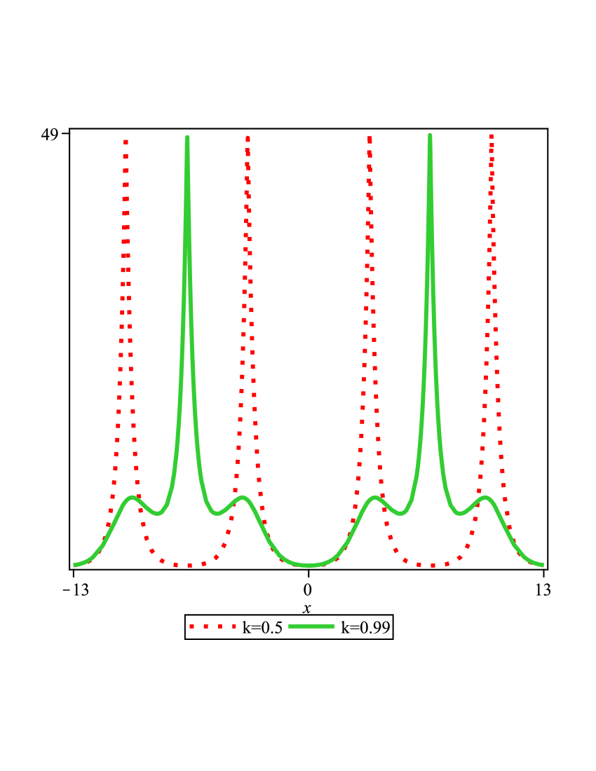
Figure 9: Solution given by (35) with $X(x)$ given by (38) and $\Phi(X)$ given by Case 6 in Table I, corresponding to (a) Plot of $\Phi(X)$ with $n=1,\,m=1/3,\,\mu=-1$, $k=0.5$ and $k=0.99$, (b) Plots of $|\psi|^{2}$ with $k=0.5$ and $k=0.99$.

In addition, it follows from Case 4 and 5 of Table I that the GP$(m,1)$ equation with $G<0$ also admits the spikon-like solutions which is similar to the case of GP$(n,n)$ equation with $G>0$. On the contrary according to Case 3 of Table I, we know that the GP$(m,1)$ equation with $G>0$ also admits the compacton-like solutions which is similar to the case of GP$(n,n)$ equation with $G<0$.

Based on the above-mentioned results, we have the following proposition:

Proposition. The nonlinear dispersive GP$(n,n)$ equation with $n>1$ possess the compacton-like solutions and spikon-like solutions. But nonlinear dispersion is not a necessary condition for the GP$(m,n)$ equation to possess these types of solutions. The linear dispersive GP$(m,1)$ equation also possess the compacton-like solutions and spikon-like solutions for $m<1$.

5.  Conclusions

In summary, we have introduced the nonlinear dispersive GP$(m,n)$ equation with the space-modulated nonlinearity and potential. By using some similarity transformations and some powerful methods, we present some families of new exact solutions with an arbitrary function $X(x)$ for different parameters $m$ and $n$. It is shown that for the nonlinear dispersion case $m=n>1$, we obtain some families of novel compacton-like solutions and spikon-like solutions of GP$(n,n)$ equation and that GP$(m,1)$ equation with linear dispersion also admits similar solutions. That is to say, nonlinear dispersion is not a necessary condition for nonlinear wave equation to allow the compacton and spikon solutions.

Although the function $X(x)$ admits the infinite kinds of choices, we focus on two special cases of Jacobi amplitude function $X(x)=c\ {\rm am}(x,k)$ and the combination of linear and trigonometric functions of $x$ to investigate the obtained solutions. In particular, for the case of Jacobi amplitude function, the corresponding compaton-like solutions can nontrivially exist on the $\mathbb{R}$ and the spikon-like solutions are shown to be localized. In addition, the nonlinearity $g(x)$ and potential $v(x)$ are both the localized period wave functions. These solutions may be useful to explain some physical phenomena.

Moreover the idea can be also extended to other nonlinear dispersive equations with varying coefficients such as the generalized GGP$(n,p,q)$ equation

$$i\frac{\partial\psi}{\partial t}=-\frac{\partial^{2}}{\partial x^{2}}(|\psi|^{n-1}\psi)+v(x)\psi+g_{p}(x)|\psi|^{p-1}\psi+g_{q}(x)|\psi|^{q-1}\psi,$$

and the three-dimensional GP$(m,n)$ equation

$$i\frac{\partial\psi}{\partial t}=-\nabla^{2}(|\psi|^{n-1}\psi)+v(x,y,z)\psi+g(x,y,z)|\psi|^{m-1}\psi,$$

where $\nabla^{2}=\partial_{x}^{2}+\partial_{y}^{2}+\partial_{z}^{2}$, which will be considered in the future.

Acknowledgements

This work was partially supported by the NSFC of China (Nos. 11071242, 61178091).

Academy of Mathematics and Systems Science, Chinese Academy of Sciences

References

- (1) M. J. Ablowitz and P. A. Clarkson, Solitons, Nonlinear Evolution Equations and Inverse Scattering (Cambridge, Cambridge University Press, 1991).
- (2) N. J. Zabusky and M. D. Kruskal, Interaction of “solitons” in a collisionless plasma and the recurrence of initial states, Phys. Rev. Lett. 15: 240-243 (1965).
- (3) G. P. Agrawal, Nonlinear fiber optics (Academic, New York, 2001).
- (4) Y. S. Kivshar and G. P. Agrawal, Optical solitons: from fibers to photonic crystals (Academic, San Diego, 2003).
- (5) A. Hasegawa and M. Matsumoto, Optical solitons in fibers (Springer, Berlin, 2003).
- (6) B. A. Malomed, Soliton management in periodic systems (Springer, New York, 2006).
- (7) A. Scott, Nonlinear science: emergence and dynamics of coherent structures, Oxford Appl. Eng. Math. Vol. 1 (Oxford, New York, 1999).
- (8) Z. Y. Yan, Nonautonomous rogons in the inhomogeneous nonlinear Schrödinger equation with variable coefficients, Phys. Lett. A 374: 672-679 (2010).
- (9) P. Rosenau and J. M. Hyman, Compactons: solitons with finite wavelength, Phys. Rev. Lett. 70: 564-567 (1993).
- (10) P. Rosenau, Nonlinear dispersion and compact structures, Phys. Rev. Lett. 73: 1737-1741 (1994)
- (11) P. Rosenau, Compact and noncompact dispersive patterns, Phys. Lett. A 275: 193-203 (1997).
- (12) F. Cooper, H. Shepard and P. Sodano, Soltary Waves and compactons in a class of generalized Korteweg-de Vries equations, Phys. Rev. E 48: 4027 (1993).
- (13) F. Cooper, J. M. Hyman and A. Khare, Compacton solutions in a class of generalized fifth-order Korteweg-de Vries equations, Phys. Rev. E 64: 026608 (2001).
- (14) B. Dey and A. Khare, Stability of compacton solutions, Phys. Rev. E 58: R2741 (1998).
- (15) B. Dey, Compacton solutions for a class of two parameter generalized odd-order KdV equations, Phys. Rev. E 57: 4733 (1998).
- (16) A. M. Wazwaz, Exact specific solutions with solitary patterns for the nonlinear dispersive K(m, n) equations, Chaos, Solitons and Fractals 13: 161-170 (2001).
- (17) Z. Y. Yan, New families of solitons with compact support for Boussinesq-like B(m,n) equations with fully nonlinear dispersion, Chaos, Solitons and Fractals 14: 1151-1158 (2002).
- (18) Z. Y. Yan and G. W. Bluman, New compacton soliton solutions and solitary patterns solutions of nonlinearly dispersive Boussinesq equations, Comput. Phys. Commun. 141: 11-18 (2002).
- (19) Y. S. Kivshar, Intrinsic localized modes as solitons with a compact support, Phys. Rev. E 48: R43-R45 (1993).
- (20) P. G. Kevrekidis and V. V. Konotop, Bright compact breathers, Phys. Rev. E 65: 066614 (2002).
- (21) P. G. Kevrekidis, V. V. Konotop, A. R. Bishop and S. Takeno, Discrete compactons: some exact results, J. Phys. A 35: L641-L642 (2002).
- (22) K. Ahnert and A. Pikovsky, Traveling waves and compactons in phase oscillator lattices, Chaos 18: 037118 (2008).
- (23) K. Ahnert and A. Pikovsky, Compactons and chaos in strongly nonlinear lattices, Phys. Rev. E 79: 026209 (2009).
- (24) P. T. Dinda and M. Remoissenet, Breather compactons in nonlinear Klein-Gordon systems, Phys. Rev. E 60: 6218-6221 (1999).
- (25) M. Eleftheriou, B. Dey, and G. P. Tsironis, Compactlike breathers: Bridging the continuous with the anticontinuous limit, Phys. Rev. E 62: 7540 (2000).
- (26) J. C. Comte, Exact discrete breather compactons in nonlinear Klein-Gordon lattices, Phys. Rev. E 65: 067601 (2002).
- (27) Z. Y. Yan, Modified nonlinearly dispersive mK(m,n,k) equations: I. New compacton solutions and solitary pattern solutions, Comput. Phys. Commun. 152: 25-33 (2003).
- (28) V. Goncharov and V. Pavlov, Model of compactons on jet streams and their collapse, Phys. Rev. E 76: 066314 (2007).
- (29) Z. Y. Yan, Envelope compactons and solitary patterns, Phys. Lett. A 355: 212-215 (2006).
- (30) Z. Y. Yan, Envelope compact and solitary pattern structures for the GNLS(m,n,p,q) equations, Phys. Lett. A 357: 196-203 (2006).
- (31) Z. Y. Yan, Exact solutions of nonlinear dispersive K(m,n) model with variable coefficients, Appl. Math. Comput. 217: 9474-9479 (2011).
- (32) A. Griffin, D. W. Snoke, and S. Stringari (Eds.) Bose-Einstein Condensations (Cambridge University Press, Cambridge, 1996).
- (33) A. S. Parkins and D. F. Walls, The physics of trapped dilute-gas Bose-Einstein condensates, Phys. Rep. 303: 1-80 (1998).
- (34) C. J. Pethick and H. Smith, Bose-Einstein Condensation in Dilute Gases (Cambridge University Press, Cambridge, 2002).
- (35) R. Carretero-González, D. J. Frantzeskakis, and P. G. Kevrekidis, Nonlinear waves in Bose-Einstein condensates: physical relevance and mathematical techniques, Nonlinearity, 21: R139 (2008).
- (36) A. J. Moerdijk, B. J. Verhaar, and A. Axelsson, Resonances in ultracold collisions of 6Li, 7Li, and 23Na, Phys. Rev. A 51: 4852-4861 (1995).
- (37) C. Chin and R. Grimm, Feshbach resonances in ultracold gases, Rev. Mod. Phys. 82: 1225-1286 (2010).
- (38) J. Belmonte-Beitia, V. M. Pérez-García, V. Vekslerchik, and P. J. Torres, Lie symmetries and solitons in nonlinear systems with spatially inhomogeneous nonlinearities, Phys. Rev. Lett. 98: 064102 (2007).
- (39) J. Belmonte-Beitia, V. M. Pérez-Garcia, V. Vekslerchik, and V. V. Konotop, Localized nonlinear waves in systems with time- and space-modulated nonlinearities, Phys. Rev. Lett. 100: 164102 (2008).
- (40) Z. Y. Yan and D. M. Jiang, Matter-wave solutions in Bose-Einstein condensates with harmonic and Gaussian potentials, Phys. Rev. E 85: 056608 (2012).
- (41) Z. Y. Yan and V. V. Konotop, Exact solutions to three-dimensional generalized nonlinear Schrödinger equations with varying potential and nonlinearities, Phys. Rev. E 80: 036607 (2009).
- (42) Z. Y. Yan, X. F. Zhang, and W. M. Liu, Nonautonomous matter waves in a waveguide, Phys. Rev. A 84: 023627 (2011).
- (43) V. M. Pérez-Garcia and R. Pardo, Localization phenomena in nonlinear Schrodinger equations with spatially inhomogeneous nonlinearities: Theory and applications to Bose-Einstein condensates, Physica D 238: 1352-1361 (2009).
- (44) D. F. Lawden, Elliptic Functions and Application (Spinger-Verlag, New York, 1989).
- (45) G. W. Bluman and S. Kumei, Symmetries and differential equations (Springer-Verlag, New York, 1989).
- (46) G. W. Bluman and Z. Y. Yan, Nonclassical potential solutions of partial differential equations, Eur. J. Appl. Math. 16: 239-261 (2005).