Exact solutions to three-dimensional generalized nonlinear Schrödinger equations with varying potential and nonlinearities

Abstract

It is shown that using the similarity transformations, a set of three-dimensional p-q nonlinear Schrödinger (NLS) equations with inhomogeneous coefficients can be reduced to one-dimensional stationary NLS equation with constant or varying coefficients, thus allowing for obtaining exact localized and periodic wave solutions. In the suggested reduction the original coordinates in the (1+3)-space are mapped into a set of one-parametric coordinate surfaces, whose parameter plays the role of the coordinate of the one-dimensional equation. We describe the algorithm of finding solutions and concentrate on power (linear and nonlinear) potentials presenting a number of case examples. Generalizations of the method are also discussed.

I Introduction

The nonlinear Schrödinger (NLS) equation is a key model describing wave processes in weakly dispersive and weakly nonlinear media Sulem . It has numerous physical applications and this universality stimulates a great deal of attention devoted to search of exact solutions of the generalized NLS models which include coefficients depending on spatial and temporal variables, i.e. describing wave dynamics in inhomogeneous media. The first exact results were obtained for the one-dimensional (1D) NLS equation using the inverse scattering technique BLR and later on generalized for the respective discrete models Discrete and to NLS with random coefficients Bisieris . Applications of the NLS equation in fiber optics have stimulated further studies of the integrable inhomogeneous models leading to the concepts of self-similar solitons and non-autonomous solitons put forward in Refs. Serkin .

Very recently the interest in exact solutions of the NLS equations with inhomogeneous coefficients was stimulated by its applications in the mean-field theory of Bose-Einstein condensate (BEC), where it is also known as Gross-Pitaevskii equation PitStrin . Except a few special cases general_inhom , the inhomogeneous NLS equation in the BEC applications appears to be nonintegrable, either due to due its two– or three–dimensional nature or in quasi-1D approximation due to the respective inhomogeneous terms (such as parabolic potentials and nonlinear inhomogeneities). Therefore new approaches, based on the self-similar transformations, have been developed. In particular, exact solutions in 1D NLS equations with stationary inhomogeneous coefficients were constructed in Refs. nontri ; BK ; Juan1 , solutions of the NLS model with coefficients depending on time and space variables were considered in Juan2 ; space-time . A $d$-dimensional NLS equation with varying coefficients was considered in PTK , where the lens transformations allowed for its reduction to the $d$-dimensional model with constant coefficients, whose dynamical properties are known. Nontrivial solutions of the cubic-quintic NLS equation with a periodic potential were also considered in 5nls . The solutions of the cubic-quintic NLS model with coefficients depending on time and space variables were addressed in Juan3 .

The present paper aims to report a possibility of generating exact solutions of a generalized three-dimensional (3D) NLS equation with inhomogeneous coefficients employing the self-similar reduction. Unlike in the previous studies we implement reduction of the spatial dimension of the system. More specifically we consider the mapping of the coordinate surfaces in the 3D space into a one-parametric family, where the quantity parameterizing the surface family serves as a variable of the 1D NLS equation with constant coefficients, thus allowing for immediate indication of a great number of exact solutions.

The solutions we will obtain have nontrivial phases, thus representing the hydrodynamic flows in specially created potentials. Bearing this in mind and taking into account that the explored potentials (parabolic and quartic) are typical for the BEC applications, we refer to such solutions also as to (exact) flows and employ the terminology widely accepted in the BEC theory.

The paper is organized as follows. In Sec. II, we describe the similarity transformation. In Sec. III, we focus on the amplitude and phase surfaces associated to the introduced transformations and present stationary solutions. Sec. IV is devoted to time-dependent cases. In Sec. V, we study the generalizations of the theory, including reduction to the 1D equations with inhomogeneous coefficients but allowing for exact solutions. The outcomes are summarized in the Conclusion.

II Similarity reductions and solutions

II.1 The similarity reduction

We concentrate on the 3D inhomogeneous p-q NLS equation with varying coefficients

$$i\frac{\partial\psi}{\partial t}=-\frac{1}{2}\nabla^{2}\psi \!\!\!+ \!\!\!v({\bf r},t)\psi$$ (1)

$$\!\!\!+ \!\!\!\left[g_{p}({\bf r},t)|\psi|^{p-1}+g_{q}({\bf r},t)|\psi|^{q-1}\right]\psi,\quad$$

where $\psi\equiv\psi({\bf r},t)$, ${\bf r}\in\mathbb{R}^{3}$, $\nabla\equiv(\partial_{x},\partial_{y},\partial_{z})$, $q>p\geq 3$ are integers, the linear potential $v({\bf r},t)$ and the nonlinear coefficients $g_{p,q}({\bf r},t)$ are all real-valued functions of time and spatial coordinates. This model contains many special types of nonlinear equations with varying coefficients such as the cubic NLS equation, the cubic-quintic NLS model, the generalized NLS model, etc.

Following the procedure suggested in Juan2 ; Yanps07 we search for a transformation connecting solutions of Eq. (1) with those of the stationary p-q NLS equation with constant coefficients

$$\mu\Phi=-\Phi_{\eta\eta}+G_{p}|\Phi|^{p-1}\Phi+G_{q}|\Phi|^{q-1}\Phi.$$ (2)

Here $\Phi\equiv\Phi(\eta)$ is a function of the only variable $\eta\equiv\eta({\bf r},t)$ whose relation to the original variables $({\bf r},t)$ is to be determined, $\mu$ is the eigenvalue of the nonlinear equation, and $G_{p,q}$ are constants. Since both $|G_{p}|$ and $|G_{q}|$ can be scaled out (by the proper renormalization of the amplitude, of $\mu$, and of the “coordinate” $\eta({\bf r},t)$) without loss of generality the consideration will be restricted to the cases where $G_{p}=0,\pm 1$ and $G_{q}=0,\pm 1$.

In order to control the boundary conditions at the infinity we impose the natural constraints

$$\eta\to 0\quad\mbox{at}\quad r\to 0\quad\mbox{and}\quad\eta\to\infty\quad\mbox{at}\quad r\to\infty.$$ (3)

Thus we consider the general similarity transformation

$$\psi({\bf r},t)=\rho({\bf r},t)e^{i\varphi({\bf r},t)}\Phi(\eta({\bf r},t)),$$ (4)

where $\varphi({\bf r},t)$ is a real-valued function and $\rho({\bf r},t)$ is a nonnegative function of the indicated variables, the both are to be determined. Requiring $\Phi(\eta)$ to be real (without loss of generality) and to satisfy Eq. (2), we substitute the ansatz (4) into Eq. (1) and after simple algebra obtain the set of equations

$$\nabla\cdot(\rho^{2}\nabla\eta)=0,$$ (5a)

$$(\rho^{2})_{t}+\nabla\cdot(\rho^{2}\nabla\varphi)=0,$$ (5b)

$$\eta_{t}+\nabla\varphi\cdot\nabla\eta=0,$$ (5c)

$$2g_{j}({\bf r},t)\rho^{j-1}-G_{j}|\nabla\eta|^{2}=0\ \ (j=p,\,q),$$ (5d)

$$2v({\bf r},t)+\mu|\nabla\eta|^{2}+|\nabla\varphi|^{2}-\rho^{-1}\nabla^{2}\rho+2\varphi_{t}=0.\qquad$$ (5e)

These equations lead to several immediate conclusions. First, it follows from (5d) that $g_{p,q}({\bf r},t)$ are sign definite, and $G_{j}={\rm sign}\{g_{j}({\bf r},t)\}$. Moreover, comparing the equations in (5d) for $j=p$ and $j=q$ we find that either $|g_{p}|=\rho^{q-p}|g_{q}|$, or one of the nonlinear coefficients is zero, i.e. either $|g_{p}|\equiv 0$ or $|g_{q}|\equiv 0$. Respectively, we define the function $g({\bf r},t)\equiv 2g_{j}\rho^{j-1}/G_{j}$, where $j=p,q$.

To solve the system (5) explicitly, we first consider the special case of $\rho({\bf r},t)$ depending only on time $t$, i.e. $\rho({\bf r},t)\equiv\rho(t)$. Then the system (5) is simplified:

$$\nabla^{2}\eta=0,$$ (6a)

$$2\rho_{t}+\rho\nabla^{2}\varphi=0,$$ (6b)

$$\eta_{t}+\nabla\varphi\cdot\nabla\eta=0,$$ (6c)

$$g({\bf r},t)-|\nabla\eta|^{2}=0,$$ (6d)

$$2v({\bf r},t)+\mu|\nabla\eta|^{2}+|\nabla\varphi|^{2}+2\varphi_{t}=0.$$ (6e)

As it is clear, the equations in the system (6) are not compatible with each other in the case of arbitrary linear and nonlinear potentials. One however can pose the problem to find functions $v({\bf r},t)$ and $g({\bf r},t)$, for which the mentioned system becomes solvable. This leads us to the procedure which can be outlined as follows.

• First, one solves Eqs. (6a)-(6c) [or Eqs. (5a)-(5c)] subject to the boundary conditions (3) what gives the functions $\eta({\bf r},t)$ and $\varphi({\bf r},t)$.

• Second, one considers Eqs. (6d) and (6e) [or Eqs. (5d) and (5e)] as definitions for the functions $v({\bf r},t)$ and $g({\bf r},t)$ through the already known $\eta({\bf r},t)$ and $\varphi({\bf r},t)$.

• Third, using one of the known solutions of the stationary p-q NLS equation (2) and the similarity transformation (4) one can construct the analytical solutions of Eq. (1).

The last step is trivially performed, taking into account that $\Phi$ is real, giving a solution in the implicit form

$$\eta=\int d\Phi\left[C-\mu\Phi^{2}+\frac{2G_{p}}{p+1}\Phi^{p+1}+\frac{2G_{q}}{q+1}\Phi^{q+1}\right]^{-\frac{1}{2}},$$ (7)

where $C$ is an integration constant.

In the next sections we implement the describe approach for a number of particular cases, relevant to the physical applications. Before that however we briefly address the issue of the integrals of motion.

II.2 One integral of motion

Integrals of motions generally appear to be the most important characteristics (either physical or mathematical) of the motion. The simplest conserved quantity for an $L^{2}$ integrable solution of the NLS equation – the number of particles, for the whole space is not defined in the case at hand, since the solutions we are dealing with do not decay at the infinity. Instead, however, as it is customary for the classical hydrodynamics dealing with flows we define a number of particles in a simply connected bounded volume $U\in\mathbb{R}^{3}$ which consists of the same ”particles” and thus moves with the ”fluid” described by the NLS equation (1), i.e. $U\equiv U(t)$:

$$N_{U}=\int_{U(t)}|\psi({\bf r},t)|^{2}d{\bf r}.$$ (8)

Under the term “particles” we understand an infinitesimal volume of the fluid moving with the velocity ${\bf v}\equiv\nabla\varphi$. Then, the solutions considered in the present paper possess the properties of the conservation of $N_{U}$:

$$\frac{dN_{U}}{dt}=0.$$ (9)

This formula represents nothing else than the well known transport formula of the conventional hydrodynamics hydro .

In order to prove (9) we first observe that it follows from Eqs. (1) and (4) that

$$\frac{\partial}{\partial t}|\psi|^{2}=-\nabla[(\rho\Phi)^{2}\nabla\varphi]\,.$$ (10)

This equation combined with the transport formula, results in the set of equalities

$$\displaystyle\frac{d}{dt}\int_{U(t)}|\psi|^{2}d{\bf r}=\displaystyle\int_{U(t)}\left[\frac{\partial}{\partial t}|\psi|^{2}+\nabla(|\psi|^{2}\cdot{\bf v})\right]d{\bf r}$$

$$=\displaystyle\int_{U(t)}\left[\frac{\partial}{\partial t}|\psi|^{2}+\nabla[(\rho\Phi)^{2}\nabla\varphi]\right]d{\bf r}=0.$$ (11)

In spite of the apparent complexity of the solutions (4), the obtained conservation of the number of particles in a material volume moving with the fluid, does not appear too surprising. Indeed, one can take into account that the symmetries of the system used to construct the solutions are based on reduction to the stationary model (2).

III Surfaces and stationary solutions

We start with the stationary solutions of Eq. (1), $\rho_{t}=\eta_{t}=\varphi_{t}=0$, imposing even more strong constrain on $\rho$ requiring it to be ${\bf r}$-independent constant. Then without loss of generality we set $\rho=1$. Also now the linear and nonlinear potentials do not depend on time $t$, i.e. $v({\bf r},t)\equiv v({\bf r})$ and $g({\bf r},t)\equiv g({\bf r})$ [recall that now it is mandatory to have $g({\bf r})>0$].

Introducing the notation $u({\bf r})\equiv-2v({\bf r})-\mu g({\bf r})$ we rewrite the system (6) in the stationary case as

$$\nabla^{2}\eta=0,\quad\nabla^{2}\varphi=0,\quad\nabla\eta\cdot\nabla\varphi=0,$$ (12a)

$$|\nabla\eta|^{2}=g({\bf r}),\quad|\nabla\varphi|^{2}=u({\bf r}).\quad\quad\quad$$ (12b)

It follows from the second of Eqs. (12b) that $u({\bf r})\geq 0$, and hence one must require $v({\bf r})\leq-\frac{1}{2}\mu g({\bf r})$.

III.1 Amplitude and phase surfaces. The potentials.

Now we consider surfaces of the constant amplitude and phase, i.e.

$$\eta({\bf r})=\eta_{0}=\mbox{const}\quad\mbox{and}\quad\varphi({\bf r})=\varphi_{0}=\mbox{const}.$$ (13)

First, we observe that the only singular points of the amplitude surfaces occur where the system becomes linear, i.e. where $g({\bf r})=0$ since otherwise $\nabla\eta({\bf r})\neq 0$. Next, having defined one of the surfaces (we will always start with the coordinate surface), the last equation in Eq.(12a) appears to be an important constraint of the definition of the other surface (in our case it will be the phase surface).

In fact, the first two equations in Eq. (12a) imply that the amplitude $\eta({\bf r})$ and phase $\varphi({\bf r})$ belong to the kernel $L=\{f({\bf r})|\nabla^{2}f({\bf r})=0\}$ of the Laplace operator $\nabla^{2}$, which are the harmonic functions and form a function space in $\mathbb{R}$. It follows from the last equation inn Eq. (12a) that the dot product of the gradients of amplitude $\eta({\bf r})$ and phase $\varphi({\bf r})$ is to zero. That is to say, $\eta({\bf r})$ and $\varphi({\bf r})$ are harmonic functions and their gradients are orthogonal.

In what follows we restrict our consideration to the finite power ($N$-order) surfaces, i.e. depending on terms like $x^{n_{1}}y^{n_{2}}z^{n_{3}}$ with $n_{j}$ being finite positive integers such that $\max\{n_{1}+n_{2}+n_{3}\}=N<\infty$. This allows us to list in the Table 1 all admissible coordinate and phase surfaces which appear to be not higher than the third-order, i.e. $N\leq 3$ (the second and third columns, respectively). The number of surfaces is limited by the irreducible cases, i.e. to the surfaces that cannot be transformed to each other by proper change of the coordinates leaving the Laplacian invariant. In all the cases the stationary phase is set zero. Notice that if the phase $\varphi({\bf r})$ is chosen as a constant, then Eq. (12a) is reduced to the single Laplace equation $\nabla^{2}\eta({\bf r})=0$ for the amplitude $\eta({\bf r})$ whose solutions are just the harmonic functions (in what follows we will not consider them).

Table 1: Admissible coordinate and phase surfaces and the respective linear and nonlinear potentials. To reduce the number of constants, those that can be scaled out by change of the coordinate units are set to one. All the constants left are real.

Case	Amplitude surface	Phase surface	Linear potential $v({\bf r})$	Nonlinear potential $g({\bf r})$
I	$\eta({\bf r})={\bf c}\cdot{\bf r}$	$\varphi({\bf r})={\bf a}\cdot{\bf r}$	$-(\mu|{\bf c}|^{2}+|{\bf a}|^{2})/2$	$|{\bf c}|^{2}$
	(plane, $|{\bf c}|\neq 0$)	(plane, $|{\bf a}|\not=0,\ {\bf c}\cdot{\bf a}=0$)	(constant)	(constant)
II	$\eta({\bf r})=x+c(y^{2}-z^{2})$	$\varphi({\bf r})=2ayz$	$-2(\mu c^{2}+a^{2})(y^{2}+z^{2})-\mu/2$	$4c^{2}(y^{2}+z^{2})+1$
	(hyperbolic paraboloid)	(hyperbolic cylinder)	(elliptic cylinder)	(elliptic cylinder)
III	$\eta({\bf r})=cx^{2}+(1-c)y^{2}-z^{2}$	$\varphi({\bf r})=2axyz$	$-2\mu[c^{2}x^{2}+(1-c)^{2}y^{2}+z^{2}]$	$4[c^{2}x^{2}+(1-c)^{2}y^{2}+z^{2}]$
	(hyperboloid of one ($c\in(0,1)$)	(third order surface)	$-2a^{2}(y^{2}z^{2}+x^{2}z^{2}+x^{2}y^{2})$	(real ellipsoid)
	or two ($c>1$) sheets and		(fourth order surface)
	hyperbolic cylinder ($c=1$))
IV	$\eta({\bf r})=xyz$	$\varphi({\bf r})=a_{1}x^{2}+a_{2}y^{2}-a_{3}z^{2}$	$-\mu(y^{2}z^{2}+x^{2}z^{2}+x^{2}y^{2})/2$	$y^{2}z^{2}+x^{2}z^{2}+x^{2}y^{2}$
	(third order surface)	(similar to $\eta({\bf r})$ in the	$-2(a_{1}^{2}x^{2}+a_{2}^{2}y^{2}+a_{3}^{2}z^{2})$	(fourth order surface)
		Case III, $a_{3}=a_{1}+a_{2}$)	(fourth order surface)

All solutions shown in Table 1 describe irrotational flows: $\nabla\times{\bf v}({\bf r})=0$ where as above ${\bf v}({\bf r})=\nabla\varphi({\bf r})$. Another feature to be emphasized is that the coordinate and phase surfaces, are defined by the linear part of the evolution equation (i.e. by the linear dispersion relation of the medium). They generate linear and nonlinear potentials. In practice however this picture is inverted: for a given linear and nonlinear potentials (created, say, experimentally) one has to introduce an appropriate coordinate surface. In this last sense the two last column in the Table 1 indicate the types of the linear and nonlinear potentials for which the mapping $(x,y,z)\to\eta$ is possible. Namely we observe that all the obtained solutions require specific quadratic and quartic linear and nonlinear potentials ($v({\bf r}),\ g({\bf r})$).

The Case I in Table 1 describes a flow with the constant velocity ${\bf v}({\bf r})=(a_{1},a_{2},a_{3})$ which is generated by the constant nonlinearity and linear potentials (the latter, obviously, can be removed). This is the trivial case of line-solutions, which by simple rotation of the coordinates are reduced to solutions depending only on one coordinate (say, $x$) and independent on other coordinates. In what follows will not consider them.

The Case II in Table 1 describes flows which are outgoing in the first and third quadrants in the $(y,z)$-plane, and incoming in the second and forth quadrants, with respect to the $x$-axis (see Fig. 1a). The velocity is given by ${\bf v}({\bf r})=(0,2az,2ay)$. Such flows is generated by the parabolic linear (either repulsive or attractive) and parabolic nonlinear potentials. Being symmetric they preserve the total number of particles.

The Case III in Table 1 is a 3D flow with the velocity ${\bf v}({\bf r})=(2ayz,2axz,2axy)$, which is generated by the quartic linear and quadratic nonlinear potentials (see Fig. 1b). In each coordinate plane, i.e. $(x,y)-$, $(x,z)-$, and $(y,z)-$plane, they all describe outgoing in the first and third quadrants, and incoming in the second and forth quadrants, flows.

The Case IV in Table 1 is a 3D flow with the velocity ${\bf v}({\bf r})=(2a_{1}x,2a_{2}y,-2(a_{1}+a_{2})z)$, which are generated by the quartic linear and quartic nonlinear potentials (see Fig. 1c).

Figure 1: (Color online) The velocity fields ${\bf v}=\nabla\varphi$ corresponding to the phases listed in Table 1 for $a=a_{1,2}=1$. (a) ($y,z$)-plane for Case II, (b) 3D-space for Case III , (c) 3D-space for Case IV.

In all the cases the types of the nonlinear interactions are determined by the constants $G_{p,q}$: they are attractive at $G_{p,q}>0$ and repulsive at $G_{p,q}<0$. Meantime the linear potential, which depends on the chemical potential is related to the type of the solution (as the different types of the solutions exist for different signs of $\mu$, see below). For $\mu<0$ the linear potentials can change the sign of their curvatures in different points of the space.

III.2 Solutions: cubic NLS equation

Following the algorithm described above, in order to construct the exact solutions of Eq. (1), as the last step we have to address solutions of Eq. (2) [i.e. the formula (7)]. They depend on the particular choice of the model. In the present work we consider two the most relevant physical cases. First we concentrate on the standard cubic NLS equation and after that we make comments on the cubic-quintic model. Thus starting with the case $p=3$, $g_{q}({\bf r})\equiv 0$ and hence $G_{q}=0$ we have to deal with the NLS equation $\mu\Phi=-\Phi_{\eta\eta}+G_{3}\Phi^{3}$. The respective periodic and localized solutions are very well known. Below we consider the simplest ones for attractive and repulsive nonlinearities $G_{3}$.

III.2.1 Attractive nonlinearity $G_{3}=-1$

Now the simplest stationary nontrivial solution is the NLS bright soliton, which gives $\psi_{bs}({\bf r})=\sqrt{-2\mu}\ {\rm sech}[\sqrt{-\mu}\,\eta({\bf r})]\exp[i\varphi]$, where $\mu<0$ and the amplitude $\eta({\bf r})$ and phase $\varphi({\bf r})$ are defined by Table 1. In Fig. 2, we display the cross-sections of the intensity $|\psi_{bs}(\eta({\bf r}))|^{2}$ of the bright soliton solution for different types of amplitude surfaces $\eta({\bf r})$ given in Table 1. We emphasize that while we use the solitonic terminology referring to the bright solitons, the respective solutions are not decaying in the 3D case we are interested in as this is illustrated by Fig. 2 (this comment on the usage of the 1D terminology is also relevant to all other solutions considered below).

We also observe that the described solutions allow for direct generalization to the p-NLS case of arbitrary even $p\geq 4$ and $G_{q}=0$ for which Eq. (2) becomes $\mu\Phi=-\Phi_{\eta\eta}+G_{p}\Phi^{p}$. The bright soliton solution of Eq. (1) obtained from (7) corresponds to $G_{p}=-1$ and $\mu=-4\omega^{2}(p-1)^{-2}$ and is given by $\psi_{pbs}({\bf r})=\left[\frac{\omega\sqrt{2(p+1)}}{p-1}\,{\rm sech}(\omega\eta({\bf r}))\right]^{2/(p-1)}e^{i\varphi({\bf r})}$, where $\omega$ is a constant.

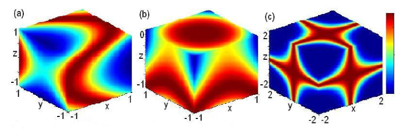
Figure 2: (Color online) Cross-sections of the density distribution of the “bright soliton” $|\psi_{bs}({\bf r})|^{2}$ with $\eta$ given in Table 1 for $\mu=-1$. (a) $c=1$ with $\eta$ for Case II, (b) $c=0.5$ with $\eta$ for Case III; here the cross-section at $z=0$ shows the peak intensity, (c) $\eta$ for Case IV.

Next we address the solutions of the 3D model (1) generated by the periodic cn-wave solution of the cubic NLS equation

$$\psi_{cn}({\bf r})=\sqrt{\frac{2\mu k^{2}}{1-2k^{2}}}\,{\rm cn}\left[\sqrt{\frac{2\mu}{1-2k^{2}}}\eta({\bf r}),k\right]e^{i\varphi({\bf r})},$$ (14)

where $k\in[0,\ 1]$ is the modulus of the Jacobi elliptic function and $\mu$ satisfies the condition $\mu(1-2k^{2})>0$, i.e. $\mu<0,\ 1/\sqrt{2}<k<1$ or $\mu>0,\ 0<k<1/\sqrt{2}$. As before the amplitude surface $\eta({\bf r})$ and phase surface $\varphi({\bf r})$ are defined by Table 1. Examples of the mentioned solutions are shown in Fig. 3.

Figure 3: (Color online) Cross-sections of the density distribution of the cn-wave solution $|\psi_{cn}({\bf r})|^{2}$ with $\eta$ given in Table 1 for $\mu=-1$. (a) $c=1$ with $\eta$ for Case II, (b) $c=0.5$ with $\eta$ for Case III, peak intensity at the center is shown by the cross-section at $z=0$, (c) $\eta$ for Case IV. In all the panels $k=0.8$.

There are two features of the solutions to be emphasized here. First, being periodic in $\eta$ the solutions are not periodic in the real 3D space. However as the “trace” of the periodicity, in Fig. 3 one observes repeated domains of maxima and minima of the density, unlike in Fig. 2, where in each cross-section one observes only one curve corresponding to the maximum of the density (which follows the projection of the amplitude surface on the plane of the chosen cross-section).

III.2.2 Repulsive nonlinearity $G_{3}=1$

This is the case where $\mu$ is positive. Now one has the dark soliton solution of Eq. (1): $\psi_{ds}({\bf r})=\sqrt{\mu}\tanh[\sqrt{\mu/2}\,\eta({\bf r})]\exp(i\varphi({\bf r}))$. The respective intensity profiles $|\psi_{ds}({\bf r})|^{2}$ are represented in Fig. 4 for different types of amplitude and phase surfaces from Table 1.

Now the linear potential is repulsive in the whole space and in center of coordinates the density becomes zero (see Fig. 4b.

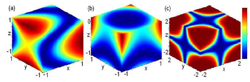
Figure 4: (Color online) Cross-sections of the density distribution of the “dark soliton” $|\psi_{ds}({\bf r})|^{2}$ with $\eta$ listed in Table 1 for $\mu=2$. (a) $c=1$ with $\eta$ for Case II, (b) $c=0.5$ with $\eta$ for Case III, the minimum intensity is shown in the cross-section with $z=0$, (c) $\eta$ for Case IV.

One can also construct “periodic” sn-wave solutions

$$\psi_{sn}({\bf r})=\sqrt{\frac{2\mu k^{2}}{1+k^{2}}}\ {\rm sn}\left[\sqrt{\frac{\mu}{1+k^{2}}}\,\eta({\bf r}),k\right]e^{i\varphi({\bf r})}$$ (15)

where we used the periodic sn-wave solution of the NLS equation with a positive chemical potential $\mu$. These solutions are depicted in Fig. 5,

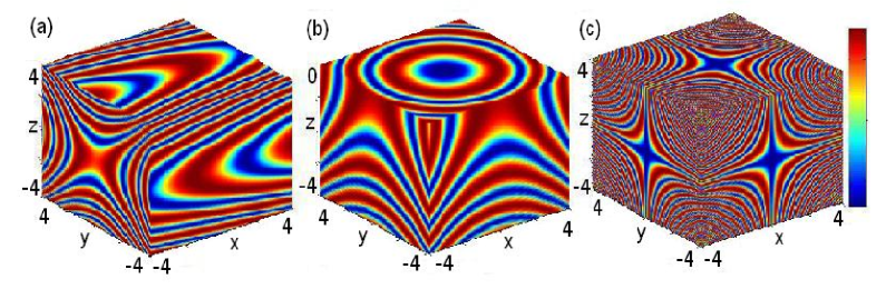
Figure 5: (Color online) Cross-sections of the density distribution of the sn-wave solution $|\psi_{sn}({\bf r})|^{2}$ with $\eta$ given in Table 1 for $\mu=2$. (a) $c=1$ with $\eta$ for Case II, (b) $c=0.5$ with $\eta$ for Case III, the minimum intensity is shown in the cross-section at $z=0$, (c) $\eta$ for Case IV. In all the panels $k=0.8$.

For other possible types of the exact flows generated by the of cubic NLS equations see e.g. Yanps .

III.3 Solutions: cubic-quintic NLS equation

Now we briefly discuss the cubic-quintic NLS equation, i.e. $p=3,\ q=5$ for which Eq. (2) becomes $\mu\Phi=-\Phi_{\eta\eta}+G_{3}\Phi^{3}+G_{5}\Phi^{5}.$ Its solutions for the condition $G_{3}G_{5}<0$ are also known (some nontrivial examples are listed in Table 3 given in Appendix A; for the methods of construction of the solutions see also Refs. Yanpla ; Yanps for more details). While the amplitude and the phase surfaces are now the same as in the case of the cubic NLS equation, the density distribution is described by different periodic and localized functions. We in particular emphasize possibility of the algebraic solutions, like the ones given by the cases 4 and 7 in Table 3.

IV Time dependent amplitudes and phase surfaces, and potentials

So far we have considered stationary solutions. Now we allow $\rho({\bf r},t)$, $\eta({\bf r},t)$ and $\varphi({\bf r},t)$ to depend on spatial and temporal variables. As before we focus on the finite power surfaces, i.e. depending on terms like $f_{n_{1}n_{2}n_{3}}(t)x^{n_{1}}y^{n_{2}}z^{n_{3}}$ with $n_{j}$ being finite positive integers such that $\max\{n_{1}+n_{2}+n_{3}\}=N<\infty$ and $f_{n_{1}n_{2}n_{3}}(t)$ being functions on time $t$. In what follows we consider all admissible coordinate and phase surfaces which appear to be not higher than the third-order, i.e. $N\leq 3$.

IV.1 Plane surface depending on time

The first nontrivial result is obtained for moving plane surfaces (which in the stationary case was reduced to the trivial 1D case). To this end, based on the Case I of the Table 1 and Eqs. (6a)-(6c) we consider $\eta$ parameterizing moving plains

$$\eta({\bf r},t)={\bf c}(t)\cdot{\bf r}$$ (16)

where ${\bf c}(t)=(c_{x}(t),c_{y}(t),c_{z}(t))$ is an arbitrary vector functions of time $t$ subject to the only constrain $c_{x}(t)c_{y}(t)c_{z}(t)>0$ for any positive time $t>0$ (this constrain, as well as similar conditions below are imposed only for the sake of simplicity). The nontrivial phase now reads

$$\varphi({\bf r},t) = {\bf r}\hat{\Omega}(t){\bf r}+{\bf a}(t)\cdot{\bf r}$$ (17)

where we have introduced the diagonal time-dependent 3$\times$3 matrix $\hat{\Omega}=$diag$(\Omega_{x},\Omega_{y},\Omega_{z})$ with $\Omega_{\sigma}=-\dot{c}_{\sigma}(t)/(2c_{\sigma}(t))$ (hereafter $\sigma=x,y,z$) and ${\bf a}(t)=(a_{x}(t),a_{y}(t),a_{z}(t))$ is a time dependent vector-function, such that the condition ${\bf c}(t)\cdot{\bf a}(t)=0$ is satisfied. Now, from Eqs. (6d) and (6e) we obtain $\rho(t)=\sqrt{c_{x}(t)c_{y}(t)c_{z}(t)},$

$$v({\bf r},t)={\bf r}\hat{A}(t){\bf r}+{\bf b}(t)\cdot{\bf r}-\frac{1}{2}(\mu|{\bf c}(t)|^{2}+|{\bf a}(t)|^{2}),$$

and $g({\bf r},t)=|{\bf c}(t)|^{2}$. Here we have defined the diagonal time-dependent 3$\times$3 matrix $\hat{A}=$diag$(A_{x},A_{y},A_{z})$ with the entries

$$A_{\sigma}=\frac{\ddot{c}_{\sigma}(t)}{2c_{\sigma}(t)}-\frac{\dot{c}_{\sigma}^{2}(t)}{c_{\sigma}^{2}(t)},$$ (18)

and the vector function ${\bf b}(t)=(b_{x},b_{y},b_{z})$ with

$$b_{\sigma}=\frac{\dot{c}_{\sigma}(t)a_{\sigma}(t)}{c_{\sigma}(t)}-\dot{a}_{\sigma}(t).$$ (19)

The described solution can be realized using the time-dependent linear potential. The nontrivial effect arising in such a geometry is that the phase surface becomes of the second order and thus the solution at hand is characterized by the inhomogeneous in space and dependent on time velocity field.

IV.2 Paraboloid depending on time

Next we consider the generalization of the parabolic Case II from the Table 1 for which the amplitude $\eta({\bf r},t)$ and the phase $\varphi({\bf r},t)$ are as follows

$$\eta({\bf r},t)=c_{x}(t)x+c_{y}(t)(y^{2}-z^{2}),$$ (20)

$$\varphi({\bf r},t)=\displaystyle{\bf r}\tilde{\Omega}(t){\bf r}+a(t)yz,$$ (21)

where as before $c_{x,y}(t)$ and $a(t)$ are functions of time such that $c_{x}(t)c_{y}(t)>0$, and we have introduced the diagonal time-dependent 3$\times$3 matrix $\tilde{\Omega}=$diag$(\Omega_{x},\Omega_{y}/2,\Omega_{z}/2)$. Now, we have $\rho(t)=\sqrt{c_{x}(t)c_{y}(t)}$, and the linear and nonlinear potentials given by

$$v({\bf r},t)={\bf r}\tilde{A}(t){\bf r}+b_{y}(t)yz-\frac{\mu}{2}c_{x}^{2}(t),$$

$$g({\bf r},t)=c_{x}^{2}(t)+4c_{y}^{2}(t)(y^{2}+z^{2}),$$

where $b_{y}(t)$ is given by Eq. (19), and we have introduced the diagonal time-dependent 3$\times$3 matrix $\tilde{A}=$diag$(A_{x},C_{y}-c_{x}^{2}/2,C_{y}-c_{x}^{2}/2)$ with $A_{x}$ and $C_{\sigma}$ being defined by Eq. (18) and

$$C_{\sigma}=\frac{2c_{\sigma}(t)\ddot{c}_{\sigma}(t)-3\dot{c}_{\sigma}^{2}(t)}{8c_{\sigma}^{2}(t)}-2\mu c_{\sigma}^{2}(t),$$ (22)

respectively.

Like in the previous case we observe that temporal evolution of the curves leads to change of the phase surface, whose position becomes $x$-dependent (c.f. the Case II in Table 1).

IV.3 Hyperboloid depending on time

Here we consider the generalization of the hyperbolic Case III from Table 1 for which the amplitude $\eta({\bf r},t)$ and phase $\varphi({\bf r},t)$ are of the forms

$$\eta({\bf r},t)={\bf r}\hat{c}(t){\bf r},$$ (23)

$$\varphi({\bf r},t)=\frac{1}{2}{\bf r}\hat{\Omega}(t){\bf r}+a(t)xyz,\ \$$ (24)

where as before $c_{\sigma}(t)$ and $a(t)$ are functions of time $t$ such that $c_{x}(t)c_{y}(t)c_{z}(t)>0$, and the condition

$$\mbox{Tr}\,\hat{c}(t)=0,$$ (25)

is required. Moreover we have introduced the diagonal time-dependent 3$\times$3 matrix $\hat{c}=$diag$(c_{x},c_{y},c_{z})$. Now we have $\rho(t)=[c_{x}(t)c_{y}(t)c_{z}(t)]^{1/4}$, and the nonlinearity $g({\bf r},t)$ and potential $v({\bf r},t)$ are given by

$$g({\bf r},t) = 4{\bf r}\hat{c}(t){\bf r},$$ (26)

$$v({\bf r},t) = {\bf r}\hat{C}(t){\bf r}-\left[a(t)\mbox{Tr}\,\hat{\Omega}(t)+\dot{a}(t)\right]xyz$$ (27)

$$\quad+\frac{1}{2}a^{2}(t)(y^{2}z^{2}+x^{2}z^{2}+x^{2}y^{2}).$$

IV.4 Third order surface depending on time

Finally we consider the time-dependent generalization of the third order surface in Case IV from the Table 1 for which the amplitude $\eta({\bf r},t)$ and phase $\varphi({\bf r},t)$ are as follows

$$\eta({\bf r},t)=c(t)xyz,$$ (28)

$$\varphi({\bf r},t)={\bf r}\hat{a}(t){\bf r},$$ (29)

where as before $c(t)$ and $a_{\sigma}(t)$ are functions of time $t$ such that $c_{x}(t)>0$ and the condition

$$\dot{c}(t)+2c(t)\mbox{Tr}\,\hat{a}(t)=0,$$ (30)

is required. Here we have introduced the diagonal time-dependent 3$\times$3 matrix $\hat{a}=$diag$(a_{x},a_{y},a_{z})$. Now $\rho(t)=\sqrt{c(t)}$, the nonlinearity $g({\bf r},t)$ and potential $v({\bf r},t)$ are as follows

$$g({\bf r},t)=c^{2}(t)(y^{2}z^{2}+x^{2}z^{2}+x^{2}y^{2}),$$ (32)

$$v({\bf r},t)={\bf r}\hat{D}(t){\bf r}-\frac{\mu}{2}c^{2}(t)(y^{2}z^{2}+x^{2}z^{2}+x^{2}y^{2}),\qquad$$

where $\hat{D}=$diag$(D_{x},D_{y},D_{z}))$ with $D_{\sigma}=-\dot{a}_{\sigma}(t)-2a_{\sigma}^{2}(t)$. Thus the introduced temporal dependence does not increase the orders of the potentials: both the linear and nonlinear potentials are quartic.

V Generalized similarity reductions and solutions

V.1 The extension of the reduction equation

The approach developed in the previous sections allows for further generalizations. Indeed, it was based on the reduction of 3D models to 1D NLS equations which admit exact solutions. The latter however need not necessarily be equations with constant coefficients. They can have either linear and/or nonlinear inhomogeneous coefficients, however still admitting exact solutions. Such situations are well known, for example for the case of periodic coefficients nontri ; BK , which can be constructed using the “inverse engineering” described in BK , and for localized and more sophisticated spatial dependencies Juan1 . Respectively, one can consider reductions of an 3D model to an inhomogeneous 1D equation with known solutions.

This leads us to the goal of this subsection: we intend to reduce Eq. (1) to the stationary p-q NLS equation with the $\eta$-modulated potentials $\mathcal{V}(\eta)$ and $\mathcal{G}_{p,q}(\eta)$

$$\mu\Phi=-\Phi_{\eta\eta}+\mathcal{V}(\eta)\Phi+\mathcal{G}_{p}(\eta)|\Phi|^{p-1}\Phi+\mathcal{G}_{q}(\eta)|\Phi|^{q-1}\Phi,$$ (33)

where $\Phi\equiv\Phi(\eta)$ is a function of the only variable $\eta\equiv\eta({\bf r},t)$ whose relation to the original variables $({\bf r},t)$ is to be determined, and $\mu$ is the eigenvalue of the nonlinear equation.

We still consider the general similarity transformation (4). Insertion of Eq. (4) into Eq. (1) and requirement that $\Phi(\eta)$ satisfies Eq. (33) yield a set of nonlinear partial differential equations, which for the amplitude and phase surfaces coincide with previously obtained ones (5a)-(5c), and for the linear and nonlinear potentials acquire the generalized form

$$\begin{array}[]{l}g_{j}({\bf r},t)=\displaystyle\frac{1}{2}\rho^{1-j}\mathcal{G}_{j}(\eta)|\nabla\eta|^{2}\quad(j=p,\,q),\vspace{0.08in}\cr v({\bf r},t)=\displaystyle\frac{1}{2}\Big{[}(V(\eta)-\mu)|\nabla\eta|^{2}-|\nabla\varphi|^{2}+\rho^{-1}\nabla^{2}\rho\Big{]}-\varphi_{t},\end{array}$$ (36)

Now we can obtain the new analytical solutions of Eq.(1) from those of Eq. (33) in terms of similarity transformation (4) and the corresponding $\eta({\bf r},t)$ and $\varphi({\bf r},t)$ given in Sec. III and IV.

Passing to examples we restrict the consideration to the cubic case $\mathcal{G}_{q}\equiv 0$ and $p=3$ and make two observations. First, being interested in flows, i.e. in solutions with varying phases and choosing a periodic linear potential $\mathcal{V}(\eta)$ in a form of the elliptic function $\mathcal{V}(\eta)=-\mathcal{V}_{0}\ {\rm sn}^{2}(\omega\eta,k),$ where $\mathcal{V}_{0}$ and $\omega$ are constants, and $k\in[0,\ 1]$ is the elliptic modulus, one can construct new 3D solutions using the respective 1D problems intensively studied in the literature (see e.g. nontri ; BK ).

Second, a new set of the solutions can be generated by the choice of the linear potential in the form

$$\mathcal{V}(\eta)=\omega^{4}\eta^{2}-\alpha^{2}\mathcal{G}_{3}(\eta)H_{n}^{2}(\omega\eta)e^{-\omega^{2}\eta^{2}},$$ (37)

where $\alpha,\omega$ are constants, $\mathcal{G}_{3}(\eta)$ is an arbitrary function of $\eta$, and $H_{n}(\omega\eta)$ is a Hermite polynomial Hermite , then one obtaines the Hermite-Gaussian solution of the nonlinear cubic Eq. (33)

$$\Phi(\eta)=\alpha H_{n}(\omega\eta)e^{-\omega^{2}\eta^{2}/2},\quad\mu=\omega^{2}(2n+1).$$ (38)

The described solution allows for direct generalization to the p-NLS case of arbitrary even $p\geq 4$ and $G_{q}=0$ for which Eq. (33) becomes

$$\mu\Phi=-\Phi_{\eta\eta}+\mathcal{V}(\eta)\Phi+\mathcal{G}_{p}(\eta)|\Phi|^{p-1}\Phi$$ (39)

whose Hermite-Gaussian solution is of the form (38) with $\mu=\omega^{2}(2n+1)$ and the chosen linear potential reads $\mathcal{V}(\eta)=\omega^{4}\eta^{2}-\alpha^{p-1}\mathcal{G}_{p}(\eta)H_{n}^{p-1}(\omega\eta)e^{(1-p)\omega^{2}\eta^{2}/2}$.

V.2 Generalized stationary reductions

The assumption that $\Phi$ is given by the expression (7), does not necessarily requires that $\rho({\bf r})$ is a constant (as this has been assumed in Sec. III). Including the coordinate dependence in the definition of $\rho$ represents another way of generalizing the results obtained above. The respective results are obtained directly from the equations (5a)-(5c), giving that now $\rho({\bf r})=\sqrt{1/f^{\prime}(\eta)}$ where $f(\eta)$ is an arbitrary function having positive derivative, $f^{\prime}\equiv df/d\eta>0$ and $\eta$ is given by one of the cases listed in the Table 1. Now $\Phi$ is obtained from the expression (7), where $\eta$ is substituted by $\tilde{\eta}=f(\eta)$. Moreover, the corresponding phase $\varphi$ is as in the stationary case (see the Table 1). This leads to the obvious modifications of the linear and nonlinear potentials directly following from Eqs. (5d) and (5e) (or Eq. (36)) .

Inversely, since the equations (5a)-(5c) for the amplitude and phase surfaces are symmetric for $\rho_{t}=\eta_{t}=\varphi_{t}=0$, for a given $\rho({\bf r})=\sqrt{1/f^{\prime}(\varphi)}$, one can hold the same amplitude surfaces, as in the stationary case (see the Table 1), with the phase being chosen as $\tilde{\varphi}=f(\varphi)$. Subsequently, this also leads to the obvious modifications of the linear and nonlinear potentials directly following from Eqs. (5d) and (5e) (or Eq. (36)).

V.3 Generalized time-dependent reductions

In addition, if we consider the general case $\rho({\bf r},t)$ in Eq. (4) depending on both time $t$ and space ${\bf r}$, then based on Eqs. (5a)-(5c) we can obtain the general amplitude $\eta({\bf r},t)$, the phase $\varphi({\bf r},t)$ and $\rho({\bf r},t)$ listed in Table 2, for which the corresponding general linear and nonlinear potentials, i.e. $g_{j}({\bf r},t)$ and $v({\bf r},t)$, can be obtained from Eq. (36). Notice that the obtained $\eta({\bf r},t),\rho({\bf r},t),\ v({\bf r},t)$ and $g_{j}({\bf r},t)$ all contain new arbitrary function $\Gamma(\zeta({\bf r},t))$, but the corresponding phases $\varphi({\bf r},t)$ have no change which are the same as ones in Sec. IV. Therefore the similarity transformation (4) containing the arbitrary function $\Gamma(\zeta({\bf r},t))$ and solutions of Eq. (33) will lead to the abundant new solution profiles of Eq. (1).

Table 2: Admissible $({\bf r},t)$-modulated amplitude and phase surfaces and $\rho({\bf r},t)$ ($\Gamma(\zeta)$ being an arbitrary differentiable function)

Case	Amplitude surface	Phase surface $\varphi({\bf r},t)$ is given by	Function $\rho({\bf r},t)$
i	$\eta({\bf r},t)=\Gamma(\zeta),\ \ \zeta={\bf c}(t)\cdot{\bf r}$	Eq.(17) with ${\bf c}(t)\cdot{\bf a}(t)=0$	$\sqrt{c_{x}(t)c_{y}(t)c_{z}(t)/\Gamma^{\prime}(\zeta)}$
ii	$\eta({\bf r},t)=\Gamma(\zeta),\ \ \zeta=c_{x}(t)x+c_{y}(t)(y^{2}-z^{2})$	Eq.(21)	$\sqrt{c_{x}(t)c_{y}(t)/\Gamma^{\prime}(\zeta)}$
iii	$\eta({\bf r},t)=\Gamma(\zeta),\ \ \zeta=c_{x}(t)x^{2}+c_{y}(t)y^{2}+c_{z}(t)z^{2}$	Eq.(24) with Eq.(25)	$\sqrt[4]{c_{x}(t)c_{y}(t)c_{z}(t)/\Gamma^{\prime 2}(\zeta)}$
iv	$\eta({\bf r},t)=\Gamma(\zeta),\ \ \zeta=c_{x}(t)xyz$	Eq.(29) with Eq.(30)	$\sqrt{c_{x}(t)/\Gamma^{\prime}(\zeta)}$

VI Conclusions

In the present work we have shown that a large diversity of 3D NLS equations with coefficients depending on time can be mapped by the proper similarity transformation into 1D models allowing for exact solution. In such reductions the original coordinates in the 1+3-space are reduced to the set of one-parametric coordinate surfaces, whose parameter plays the role of the coordinate of the new 1D equation. When the obtained equation allows for exact solutions, the respective solutions of the original 3D model can be constructed immediately using different types of the admissible coordinate surfaces.

We considered power surfaces, which give origin to parabolic and quartic linear and nonlinear potentials. Such potentials are typical for the physical applications in the nonlinear optics and in the mean-field theory of Bose-Einstein condensates, what determines the large range of the possible applications of the found solutions, as well as of the method itself.

We also point out that not only the exact solutions itself represent the major interest. As the 3D equation is reduce to the 1D model one can consider the existence of the solutions of the original model on the basis of the known existence of the reduced equation. So, for example, 1D NLS equations with periodic linear and nonlinear potentials  BluKon or with a parabolic linear AlZez potential allow for existence of various branches of the solutions (which however can be found only numerically). Each of the branches can be parameterized by the frequency (or energy, or chemical potential, depending on the applications), and this leads to a parametric set of the 3D NLS equations with inhomogeneous potentials allowing for either localized or periodic solutions. In addition, the reported method can be also extended to the 3D (or $d$-dimensional) p-q NLS equation (or coupled p-q NLS equations) with varying potentials, nonlinearities, dispersions and gain/loss terms PTK ; Mal ; RDP ; Bel .

We however, left open several relevant questions. Among them we mention the stability of the obtained solutions which hardly can be implemented with the framework of a general scheme, similar to one used to obtain the solutions. We also did not discuss the relation between the self-similar flows obtained in the present paper and collapsing solutions, for which the similarity transformation (usually referred to as lens transformation) appears to be a powerful tool Berge . The complexity of this last issue is determent by the presence of inhomogeneous end even time-dependent linear an nonlinear potentials, requiring further detail study.

Appendix A Appendix

For the sake of convenience here we present several exact solutions of the cubic-quintic NLS equation (2) with $p=3,\,q=5$, which are listed in Table 3.

Table 3: Solutions for the case cubic-quintic NLS equation ($k^{\prime 2}=1-k^{2}$)

Case	$G_{3}$	$G_{5}$	$\mu$	$\omega^{2}$	$\Phi(\eta)$
1	$\ \ 1$	$-1$	$3(4k^{2}+1)/(64k^{2})$	$3/(16k^{2})$	$3/8\big{[}1+{\rm cn}(\omega\eta,k)\big{]}^{1/2}$
2	$\ \ 1$	$-1$	$-2$	$3/2$	$\displaystyle\sqrt{7}\cos(\omega\eta)\big{[}9-7\cos^{2}(\omega\eta)\big{]}^{-1/2}$
3	$\ \ 1$	$-1$	$\omega^{2}(2k^{2}-1)/2-5/4$	$\big{[}2(1-2k^{2})+\sqrt{4(1-2k^{2})^{2}+45}\ \big{]}/6$	$\displaystyle\frac{\sqrt{10}k\ {\rm cn}(\omega\eta,k)}{\big{[}3(2\omega^{2}+6k^{2}-3)-10k^{2}\ {\rm cn}^{2}(\omega\eta,k)\big{]}^{1/2}}$
4	$\ \ 1$	$-1$	$0$	$1$	$\sqrt{6}\ \big{[}4+3\eta^{2}\big{]}^{-1/2}$
5	$-1$	$\ \ 1$	$3(k^{2}-5)/64$	$3/16$	$3/8\big{[}1+k\ {\rm sn}(\omega\eta,k)\big{]}^{1/2}$
6	$-1$	$\ \ 1$	$-\omega^{2}(k^{2}+1)/2+5/4$	$\big{[}-2(1+k^{2})+\sqrt{4(1+k^{2})^{2}+45k^{\prime 4}}\ \big{]}/(6k^{\prime 4})$	$\displaystyle\frac{\sqrt{10}k\ {\rm sn}(\omega\eta,k)}{\big{[}6\omega^{2}k^{\prime 4}+9(k^{2}+1)-10k^{2}{\rm sn}^{2}(\omega\eta,k)\big{]}^{1/2}}$
7	$-1$	$\ \ 1$	$1/4$	$1$	$\eta\big{[}24+2\eta^{2}\big{]}^{-1/2}$

References

- (1) C. Sulem and P. L. Sulem The Nonlinear Schrödinger Equation : Self-focusing and Wave Collapse (Springer-Verlag, New York, 1999).
- (2) H.-H. Chen and C.-S. Liu, Phys. Rev. Lett. 37, 693 (1976).
- (3) M. Bruschi, D. Levi, and O. Ragnisco, IL Nuovo Cimento A 53, 21 (1979); R. Scharf and A. R. Bishop, Phys. Rev. A 43, 6535 (1991); V. V. Konotop, O. A. Chubykalo, and L. Vázquez, Phys. Rev. E 48, 563 (1993); V. V. Konotop, Theor. Math. Phys. 99, 687 (1994).
- (4) I. M. Besieris, in Nonlinear Electromagnetics Ed. P.L.E. Uslenghi (Academic Press, New York, 1980); see also V. V. Konotop and L. Vázquez Nonlinear Random Waves (World Scientific Publishing, Singapore, 1994).
- (5) V. N. Serkin, and A. Hasegawa, Phys. Rev. Lett. 85, 4502 (2000); V. N. Serkin and A. Hasegawa, IEEE J. Select. Topics Quantum Electron 8, 418 (2002); S. Chen, and L. Yi, Phys. Rev. E 71 (2005) 016606; S. A. Ponomarenko and G. P. Agrawal, Phys. Rev. Lett. 97, 013901 (2006); V. N. Serkin, A. Hasegawa and T. L. Belyaeva, Phys. Rev. Lett. 98, 074102 (2007).
- (6) L. Pitaevskii and S Stringari, Bose-Einstein Condensation (Oxford University Press, Oxford, 2003).
- (7) Z. X. Liang, Z. D. Zhang, and W. M. Liu, Phys. Rev. Lett. 94, 050402 (2005).
- (8) J. C. Bronski, L. D. Carr, B. Deconinck, J. N. Kutz and K. Promislow, Phys. Rev. E 63, 036612 (2001); J. C. Bronski, L. D. Carr, R. Carretero-Gonzalez, B. Deconinck, J. N. Kutz and K. Promislow, Phys. Rev. E 64, 056615 (2001).
- (9) V. A. Brazhnyi and V. V. Konotop, Mod. Phys. Lett. B 18, 627 (2004).
- (10) J. Belmonte-Beitia, V. M. Pérez-Garcia, V. Vekslerchik, and P. J. Torres, Phys. Rev. Lett. 98, 064102 (2007).
- (11) J. Belmonte-Beitia, V. M. Pérez-García, V. Vekslerchik, and V. V. Konotop, Phys. Rev. Lett. 100, 164102 (2008).
- (12) D. Zhao, H.-G. Luo, and H.-Y. Chai, Phys. Lett. A 372, 5644 (2008); A. T. Avelar, D. Bazeia, and W. B. Cardoso, Phys. Rev. E 79, 025602(R) (2009).
- (13) V. M. Pérez-García, P. J. Torres, and V. V. Konotop, Physica D 221, 31 (2006).
- (14) E. Kengne, R. Vaillancourt, and B. A. Malomed, J. Phys. B 41, 205202 (2008).
- (15) J. Belmonte-Beitia, and J. Cuevas, J. Phys. A 42, 165201 (2009).
- (16) Z. Y. Yan, Phys. Scr. 75, 320 (2007).
- (17) see e.g. A. J. Majda and A. L. Bertozzi Vorticity and Incompressible Flow (Cambridge University Press, Cambridge, 2002)
- (18) Yu. V. Bludov and V. V. Konotop, Phys. Rev. A 74, 043616 (2006).
- (19) G. L. Alfimov and D. A. Zezyulin, Nonlinearity 20, 2075 (2007).
- (20) M. Abramowitz and I. A. Stegun, Handbook of Mathematical Functions (Dover Publications, Inc., New York, 1965)
- (21) Z. Y. Yan, Phys. Lett. A 331, 193 (2004); Z. Y. Yan, Constructive Theory and Applications of Complex Nonlinear Waves (Science Press, Beijing, 2007).
- (22) Z. Y. Yan, Phys. Scr. 78, 035001 (2008).
- (23) B. A. Malomed, D. Mihalache, F. Wise, and L. Torner, J. Opt. B: Quantum Semiclass. Opt. 7, R53 (2005).
- (24) R. Carretero-González, D. J. Frantzeskakis, and P. G. Kevrekidis, Nonlinearity 21, R139 (2008).
- (25) M. Belić, N. Petrović, W. P. Zhong, R. H. Xie, and G. Chen, Phys. Rev. Lett. 101, 123904 (2008).
- (26) L. Berge, Phys. Rep. 303, 259 (1998)