Noisy Tensor Completion for Tensors with a Sparse Canonical Polyadic Factor

Abstract

In this paper we study the problem of noisy tensor completion for tensors that admit a canonical polyadic or CANDECOMP/PARAFAC (CP) decomposition with one of the factors being sparse. We present general theoretical error bounds for an estimate obtained by using a complexity-regularized maximum likelihood principle and then instantiate these bounds for the case of additive white Gaussian noise. We also provide an ADMM-type algorithm for solving the complexity-regularized maximum likelihood problem and validate the theoretical finding via experiments on synthetic data set.

Tensor decomposition, noisy tensor completion, complexity-regularized maximum likelihood estimation, sparse CP decomposition, sparse factor models.

I Introduction

The last decade has seen enormous progress in both the theory and practical solutions to the problem of matrix completion, in which the goal is to estimate missing elements of a matrix given measurements at some subset of its locations. Originally viewed from a combinatorial perspective [1], it is now usually approached from a statistical perspective in which additional structural assumptions (e.g., low-rank, sparse factors etc) not only make the problem tractable but allow for provable error bounds from noisy measurements [2, 3, 4, 5, 6, 7, 8]. Tensors, which we will view as multi-way arrays, naturally arise in slew of practical applications in the areas of signal processing, computer vision, neuroscience, etc. [9, 10]. Often in practice tensor data is collected in a noisy environment and suffers from missing observations. Given the success of matrix completion methods, it is no surprise that recently there has been a lot of interest in extending the successes of matrix completion to tensor completion problem [11, 12, 13].

In this work we consider the general problem of tensor completion. Let $\underline{X}^{*}\in\mathbb{R}^{n_{1}\times n_{2}\times n_{3}}$ be the tensor we wish to estimate and suppose we collect the noisy measurements $Y_{i,j,k}$ at subset of its location $(i,j,k)\in\mathcal{S}\subset[n_{1}]\times[n_{2}]\times[n_{3}]$. The goal of tensor completion problem is to estimate the tensor $\underline{X}^{*}$ from noisy observations $\{\underline{Y}_{i,j,k}\}_{(i,j,k)\in\mathcal{S}}$. This problem is naturally ill-posed without any further assumption on the tensor we wish to estimate. We focus on structured tensors that admit “sparse CP decomposition” by which we mean that one of the canonical polyadic or CANDECOMP/PARAFAC (CP)-factors (defined in section I-D) is sparse. Tensors admitting such structure arise in many applications involving electroencephalography (EEG) data, neuroimaging using functional magnetic resonance imaging (MRI), and many others [14, 15, 13, 16, 17].

I-A Our Contributions

Our main contribution is encapsulated by Theorem 1 which provides general estimation error bounds for noisy tensor completion via complexity-regularized maximum likelihood estimation[18, 19] for tensors fitting our data model. This theorem can be instantiated for specific noise distributions of interest, which we do for the case when the observations are corrupted with additive white Gaussian noise. We also provide a general ADMM-type algorithm which solves an approximation to the problem of interest and then provide numerical evidence validating the statistical convergence rates predicted by Theorem 1.

I-B Relation with existing works

A common theme of recent tensor completion works is modifying the tools that have been effective in tackling the matrix completion problem to apply to tensors. For example, one could apply matrix completion results to tensors directly by matricizing the tensors along various modes and minimizing the sum or weighted sum of their nuclear norms as a convex proxy for tensor rank [20, 21, 22]. Since the nuclear norm is computationally intractable for large scale data, matrix completion via alternating minimization was extended to tensors in [23, 24].

In contrast to these works, in this paper we consider the noisy completion of tensors that admit a CP decomposition with one of the factors being sparse. Recently, the completion of tensors with this model was exploited in the context of time series prediction of incomplete EEG data [13]. Our work is focussed on providing recovery guarantees and a general algorithmic framework and draws inspiration from recent work on noisy matrix completion under a sparse factor model [8] and extends it to tensors with a sparse CP factor.

I-C Outline

After an overview of the notation used in this paper in section II we present the problem setup. In section III we present our main theorem and instantiate it for the case of Gaussian noise. In section IV we provide the algorithmic framework to solve the complexity regularized maximum likelihood estimation. Numerical experiments are provided in section VI, followed by a brief discussion and future research directions in section VII.

I-D Notation

Given two continuous random variables $X\sim p(x)$ and $Y\sim q(y)$ defined on the same probability space and with $p$ absolutely continuous with respect to $q$, we define the Kullback-Leibler divergence (KL-divergence) of $q$ from $p$ to be

$$D(p\|q)=\mathbb{E}_{p}\left[\log\frac{p}{q}\right].$$

If $p$ is not absolutely continuous with respect to $p$, then define $D(p\|q)=\infty$. The Hellinger affinity of two distributions is similarly defined by

$$A(p,q)=\mathbb{E}_{p}\left[\sqrt{\frac{q}{p}}\right]=\mathbb{E}_{q}\left[\sqrt{\frac{p}{q}}\right].$$

We will denote vectors with lower-case letters, matrices using upper-case letters and tensors as underlined upper-case letters (e.g., $v\in\mathbb{R}^{n},A\in\mathbb{R}^{m\times n},$ and $\underline{X}\in\mathbb{R}^{n_{1}\times n_{2}\times n_{3}}$, respectively). Furthermore, for any vector (or matrix) $v\in\mathbb{R}^{n}$ define $\left\|v\right\|_{0}=\left|\{i:v_{i}\neq 0\}\right|$ to be the number of non-zero elements of $v$ and $\|v\|_{\infty}:=\max_{i}\left\{\left|v_{i}\right|\right\}$ to denote maximum absolute of $v$. Note that $\left\|A\right\|_{\infty}:=\max_{i,j}\left\{\left|A_{i,j}\right|\right\}$ is not the induced norm of the matrix $A$. Entry $(i,j,k)$ of tensor $\underline{X}$ will be denoted by $X_{i,j,k}$. For a tensor $\underline{X}$ we define its Frobenius norm in analogy with the matrix case as $\left\|\underline{X}\right\|_{F}^{2}=\sum_{i,j,k}X_{i,j,k}^{2}$ the squared two norm of its vectorization and its maximum absolute entry as $\|\underline{X}\|_{\infty}=\max_{i,j,k}|\underline{X}_{i,j,k}|$. Finally, we define the canonical polyadic or CANDECOMP/PARAFAC (CP) decomposition of a tensor $\underline{X}\in\mathbb{R}^{n_{1}\times n_{2}\times n_{3}}$ to be a representation

$$\underline{X}=\sum_{f=1}^{F}a_{f}\circ b_{f}\circ c_{f}=:[A,B,C],$$ (1)

where $a_{f},b_{f},$ and $c_{f}$ are the $f^{th}$ columns of $A,B,$ and $C$, respectively, $a_{f}\circ b_{f}\circ c_{f}$ denotes the tensor outer product such that $(a_{f}\circ b_{f}\circ c_{f})_{i,j,k}=(i^{th}\textrm{ entry of }a_{f})\times(j^{th}\textrm{ entry of }b_{f})\times(k^{th}\textrm{ entry of }c_{f})$, and $[A,B,C]$ is the shorthand notation of $\underline{X}$ in terms of its CP factors. The parameter $F$ is an upper bound on the rank of $\underline{X}$ (we refer the reader to [10] for a comprehensive overview of tensor decompositions and their uses). For a given tensor $\underline{X}$ and CP decomposition $[A,B,C]$ define $n_{\max}=\max\{n_{1},n_{2},n_{3},F\}$ as the maximum dimension of its CP factors and number of latent factors.

II Problem Setup

II-A Data model

Let $\underline{X}^{*}\in\mathcal{X}\subset\mathbb{R}^{n_{1}\times n_{2}\times n_{3}}$ be the unknown tensor whose entries we wish to estimate. We assume that $X^{*}$ admits a CP decomposition such that the CP factors $A^{*}\in\mathbb{R}^{n_{1}\times F}$, $B^{*}\in\mathbb{R}^{n_{2}\times F}$, $C^{*}\in\mathbb{R}^{n_{3}\times F}$ are entry-wise bounded: $\|A^{*}\|_{\infty}\leq A_{\max}$, $\|B^{*}\|_{\infty}\leq B_{\max}$, $\|C^{*}\|_{\infty}\leq C_{\max}$. Furthermore, we will assume that $C^{*}$ is sparse $\|C^{*}\|_{0}\leq k$. Then $\underline{X}^{*}$ can be decomposed as follow

$$\underline{X}^{*}=[A^{*},B^{*},C^{*}]=\sum_{f=1}^{F}a_{f}^{*}\circ b_{f}^{*}\circ c_{f}^{*}.$$

$\underline{X}$ is also entry-wise bounded, say by $\|\underline{X}^{*}\|_{\infty}\leq\frac{X_{\max}}{2}$. Such tensors have a rank upper bounded by $F$.

II-B Observation setup

We assume that we measure a noisy version of $\underline{X}^{*}$ at some random subset of the entries $S\subset[n_{1}]\times[n_{2}]\times[n_{3}]$. We generate $S$ via an independent Bernoulli model with parameter $\gamma\in(0,1]$ as follows: first generate $n_{1}n_{2}n_{3}$ i.i.d.  Bernoulli random variables $b_{i,j,k}$ with $\textrm{Prob}(b_{i,j,k}=1)=\gamma,\forall i,j,k$ and then the set $S$ is obtained as $S=\{(i,j,k):b_{i,j,k}=1\}$. Conditioned on $S$, in the case of an additive noise model we obtain noisy observations at the locations of $S$ as follows

$$\underline{Y}_{i,j,k}=\underline{X}_{i,j,k}^{*}+n_{i,j,k},\quad\forall(i,j,k)\in S,$$ (2)

where $n_{i,j,k}$’s are the i.i.d noise entries.

II-C Estimation procedure

Our goal here is to obtain an estimate for full true tensor $\underline{X}^{*}$ using the noisy sub-sampled measurement $\underline{Y}_{i,j,k}$. We pursue the complexity-regularized maximum likelihood to achieve this goal. For this we first note that the observations $\underline{Y}_{i,j,k}$ have distribution parameterized by the entries of the true tensor $\underline{X}^{*}$ and the overall likelihood is given by

$$p_{\underline{X}^{*}_{S}}(\underline{Y}_{S}):=\prod_{(i,j,k)\in S}p_{\underline{X}_{i,j,k}^{*}}(\underline{Y}_{i,j,k}).$$ (3)

where $p_{\underline{X}_{i,j,k}^{*}}(\underline{Y}_{i,j,k})$ is the pdf of observation $Y_{i,j,k}$ which depends on the pdf of the noise and is parametrized by $X_{i,j,k}^{*}$. We use the shorthand notation $\underline{X}_{S}$ to denote the entries of the tensor $\underline{X}$ sampled at the indices in $S$.

Using prior information that $C$ is sparse, we regularize with respect to the sparsity of $C$ and obtain the complexity-regularized maximum likelihood estimate $\hat{\underline{X}}$ of $\underline{X}^{*}$ as given below

$$\hat{{\underline{X}}}=\operatorname*{\arg\,\min}_{\underline{X}=[A,B,C]\in\mathcal{X}}\left(-\log p_{\underline{X}_{S}}(Y_{S})+\lambda\left\|C\right\|_{0}\right),$$ (4)

where $\lambda>0$ is the regularization parameter and $\mathcal{X}$ is a class of candidate estimates. Specifically, we take $\mathcal{X}$ to be a finite class of estimates constructed as follows: first choose some $\beta\geq 1$, and set $L_{\rm lev}=2^{\lceil\log_{2}(n_{max})^{\beta}\rceil}$ and construct $\mathcal{A}$ to be the set of all matrices $A\in\mathbb{R}^{n_{1}\times F}$ whose elements are discretized to one of $L_{\rm lev}$ uniformly spaced between $[-A_{\max},A_{\max}]$, similarly construct $\mathcal{B}$ to be the set of all matrices $B\in\mathbb{R}^{n_{2}\times F}$ whose elements are discretized to one of $L_{\rm lev}$ uniformly spaced between $[-B_{\max},B_{\max}]$, finally $\mathcal{C}$ be the set of matrices $C\in\mathbb{R}^{n_{3}\times F}$ whose elements are either zero or are discretized to one of $L_{\rm lev}$ uniformly spaced between $[-C_{\max},C_{\max}]$. Then, we let

$$\mathcal{X}^{\prime}=\left\{[A,B,C]\bigg{|}A\in\mathcal{A},B\in\mathcal{B},C\in\mathcal{C},\|\underline{X}\|_{\infty}\leq X_{\max}\vphantom{\sum_{f=1}^{F}a_{f}\circ b_{f}\circ c_{f}}\right\}$$ (5)

and we let $\mathcal{X}$ be any subset of $\mathcal{X}^{\prime}$.

III Main result

In this section we present the main result in which we provide an upper bound on the quality of the estimate obtained by solving (4).

Theorem 1.

Let $S$ be sampled according to the independent Bernoulli model with parameter $\gamma=\frac{m}{n_{1}n_{2}n_{3}}$ and let $Y_{S}$ be given by (3). Let $Q_{D}$ be any upper bound on the maximum KL divergence between $p_{\underline{X}^{*}_{i,j,k}}$ and $p_{\underline{X}_{i,j,k}}$ for $\underline{X}\in\mathcal{X}$

$$Q_{D}\geq\max_{\underline{X}\in\mathcal{X}}\max_{i,j,k}D\left(p_{\underline{X}^{*}_{i,j,k}}\big{\|}p_{\underline{X}_{i,j,k}}\right)$$

where $\mathcal{X}$ is as defined in (4). Then for any $\lambda$ satisfying

$$\lambda\geq 4\left(\beta+2\right)\left(1+\frac{2Q}{3}\right)\log n_{max}$$ (6)

the regularized constrained maximum likelihood estimate $\underline{\hat{X}}$ obtained from (4) satisfies

$$\frac{\mathbb{E}_{S,Y_{S}}\left[-2\log(A(p_{\underline{\hat{X}}},p_{\underline{X}^{*}}))\right]}{n_{1}n_{2}n_{3}}$$

$$\leq 3\min_{\underline{X}\in\mathcal{X}}\left\{\frac{D(p_{\underline{X}^{*}}\|p_{\underline{X}})}{n_{1}n_{2}n_{3}}+\left(\lambda+\frac{8Q_{D}(\beta+2)\log n_{max}}{3}\right)\right.$$

$$\left.\qquad\qquad\quad\quad\quad\quad\frac{(n_{1}+n_{2})F+\|C\|_{0}}{m}\right\}+\frac{8Q_{D}\log m}{m}.$$

Proof.

The proof appears in the appendix section IX-A. ∎

The above theorem extends the main result of [8] to the tensor case. It states a general result relating the log affinity between the distributions parameterized by the estimated tensor and the ground truth tensor. Hellinger affinity is a measure of distance between two probability distributions which can be used to get bounds on the quality of the estimate. As in [8], the main utility of this theorem is that it can be instantiated for noise distributions of interest such as Gaussian, Laplace and Poisson. Note that since the estimation procedure depends only on the likelihood term, the above theorem can also be extended to non-linear observation models such as 1-bit quantized measurements [8]. We next demonstrate the utility of the above theorem to present error guarantees when the additive noise follows a Gaussian distribution.

III-A Gaussian Noise Case

We examine the implications of Theorem 1 in a setting where observations are corrupted by independent additive zero-mean Gaussian noise with known variance. In this case, the observations $Y_{S}$ are distributed according to a multivariate Gaussian density of dimension $|S|$ whose mean corresponds to the tensor entries at the sample locations and with covariance matrix $\sigma^{2}I_{|S|}$, where $I_{|S|}$ is the identity matrix of dimension $|S|$. That is,

$$p_{\underline{X}^{*}_{S}}(\underline{Y}_{S})=\frac{1}{(2\pi\sigma^{2})^{|S|/2}}\exp\left(-\frac{1}{2\sigma^{2}}\ \|\underline{Y}_{S}-\underline{X}^{*}_{S}\|_{F}^{2}\right),$$ (8)

In order to apply Theorem 1 we choose $\beta$ as:

$$\beta=\max\left\{1,1+\frac{\log\left(\frac{14FA_{\max}B_{\max}C_{\max}}{X_{\max}}+1\right)}{\log(n_{\max})}\right\}$$ (9)

Then, we fix $\mathcal{X}=\mathcal{X}^{\prime}$, and obtain an estimate according to (4) with the $\lambda$ value chosen as

$$\lambda=4\left(1+\frac{2Q_{D}}{3}\right)(\beta+2)\cdot\log(n_{\max})$$ (10)

In this setting we have the following result.

Corollary 1.

Let $\beta$ be as in (9), let $\lambda$ be as in (10) with $Q_{D}=2X_{\max}^{2}/\sigma^{2}$, and let $\mathcal{X}=\mathcal{X}^{\prime}$. The estimate $\widehat{\underline{X}}$ obtained via (4) satisfies

$$\begin{split}&\frac{\mathbb{E}_{S,Y_{S}}\left[\|\underline{X}^{*}-\widehat{\underline{X}}\|_{F}^{2}\right]}{n_{1}n_{2}n_{3}}=\\ &\quad\quad{\cal O}\left(\vphantom{\left(\frac{(n_{1}+n_{2})F+\|C^{*}\|_{0}}{m}\right)}\log(n_{\max})(\sigma^{2}+X_{\max}^{2})\right.\left.\left(\frac{(n_{1}+n_{2})F+\|C^{*}\|_{0}}{m}\right)\right).\end{split}$$ (11)

Proof.

The proof appears in appendix section IX-C. ∎

Remark 1.

The quantity $(n_{1}+n_{2})F+\left\|C^{*}\right\|_{0}$ can be viewed as the number of degrees of freedom of the model. In this context, we note that our estimation error is proportional to the number of degrees of freedom of the model divided by $m$ multiplied by the logarithmic factor $\log(n_{\max})$.

Remark 2.

If we were to ignore the multilinear structure and matricize the tensor as

$$X^{*}_{(3)}=(B^{*}\odot A^{*})(C^{*})^{T},$$

where $\odot$ is the Khatri-Rao product (for details of matricization refer [9]) and apply the results from [8] we would obtain the bound

$$\begin{split}&\frac{\mathbb{E}_{S,Y_{S}}\left[\|\underline{X}^{*}-\widehat{\underline{X}}\|_{F}^{2}\right]}{n_{1}n_{2}n_{3}}=\\ &\quad\quad{\cal O}\left(\log(n_{\max})(\sigma^{2}+X_{\max}^{2})\left(\frac{(n_{1}\cdot n_{2})F+\|C^{*}\|_{0}}{m}\right)\right),\end{split}$$

That is, the factor of $(n_{1}+n_{2})F$ in Theorem 1 has become a factor of ($n_{1}\cdot n_{2})F$ when matricizing, a potentially massive improvement.

IV The Algorithmic framework

In this section we propose an ADMM-type algorithm to solve the complexity regularized maximum likelihood estimate problem in (4). We note that the feasible set $\mathcal{X}$ problem in (4) is discrete which makes the algorithm design difficult. Similar to [8] we drop the discrete assumption in order to use continuous optimization techniques. This may be justified by choosing a very large value of $L_{\rm lev}$ and by noting that continuous optimization algorithms, when executed on a computer, use finite precision arithmetic, and thus a discrete set of points. Hence, we consider the design of an optimization algorithm for the following problem:

$$\min_{\underline{X},A,B,C}-\log p_{\underline{X}_{S}}(\underline{Y}_{S})+\lambda\left\|C\right\|_{0}$$ (12)

$$\text{subject to}\quad A\in\mathcal{A},B\in\mathcal{B},C\in\mathcal{C},$$

$$\qquad\qquad\left\|\underline{X}\right\|_{\infty}\leq X_{\max},\underline{X}=\sum_{f=1}^{F}a_{f}\circ b_{f}\circ c_{f},$$

$$\qquad\qquad\mathcal{A}=\left\{A\in\mathbb{R}^{n_{1}\times F}:\left\|A\right\|_{\infty}\leq A_{\max}\right\},$$

$$\qquad\qquad\mathcal{B}=\left\{B\in\mathbb{R}^{n_{2}\times F}:\left\|B\right\|_{\infty}\leq B_{\max}\right\},$$

$$\qquad\qquad\mathcal{C}=\left\{C\in\mathbb{R}^{n_{3}\times F}:\left\|C\right\|_{\infty}\leq C_{\max}\right\}.$$

We form the augmented Lagrangian for the above problem

$$\mathcal{L}(\underline{X},A,B,C,\lambda)=-\log p_{\underline{X}_{S}}(\underline{Y}_{S})+\lambda\left\|C\right\|_{0}+$$

$$\frac{\rho}{2}\left\|\underline{X}-\sum_{f=1}^{F}a_{f}\circ b_{f}\circ c_{f}\right\|_{F}^{2}+\lambda^{T}\cdot\operatorname{vec}\left(\underline{X}-[A,B,C]\right)$$

$$+I_{\mathcal{X}}(\underline{X})+I_{\mathcal{A}}(A)+I_{\mathcal{B}}(B)+I_{\mathcal{C}}(C),$$

where $\lambda$ is Lagrangian vector of size $n_{1}n_{2}n_{3}$ for the tensor equality constraint and $I_{\mathcal{X}}(\underline{X}),I_{\mathcal{A}}(A),I_{\mathcal{B}}(B),I_{\mathcal{C}}(C)$ are indicator functions of the sets $\|\underline{X}\|_{\infty}\leq X_{\max}$, $\mathcal{A}$, $\mathcal{B}$, $\mathcal{C}$ respectively. Starting from the augmented Lagrangian we extend the ADMM-type algorithm proposed in [8] to the tensor case as shown in Algorithm 1.

V The algorithm

Algorithm 1 ADMM-type algorithm for noisy tensor completion

Inputs: $\Delta_{1}^{\rm stop},\Delta_{2}^{\rm stop},\eta,\rho^{(0)}$
Initialize: $\underline{X}^{(0)}$, $A^{(0)}$,$B^{(0)}$,$C^{(0)}$, $\lambda^{(0)}$

while $\Delta_{1}>\Delta_{1}^{\rm stop},\Delta_{2}>\Delta_{2}^{\rm stop},t\leq t_{max}$ do

    S1: $\underline{X}^{(t+1)}=\operatorname*{\arg\,\min}_{\underline{X}}\mathcal{L}(\underline{X},A^{(t)},B^{(t)},C^{(t)},\lambda^{(t)})$

    S2: $A^{(t+1)}=\operatorname*{\arg\,\min}_{A}\mathcal{L}(\underline{X}^{(t+1)},A,B^{(t)},C^{(t)},\lambda^{(t)})$

    S3: $B^{(t+1)}=\operatorname*{\arg\,\min}_{B}\mathcal{L}(\underline{X}^{(t+1)},A^{(t+1)},B,C^{(t)},\lambda^{(t)})$

    S4: $C^{(t+1)}=\operatorname*{\arg\,\min}_{C}\mathcal{L}(\underline{X}^{(t+1)},A^{(t+1)},B^{(t+1)},C,\lambda^{(t)})$

    S5: $\lambda^{(t+1)}=\lambda^{(t)}+\rho^{(0)}\operatorname{vec}\left(\underline{X}^{(t+1)}-[A^{(t+1)},B^{(t+1)},C^{(t+1)}]\right)$

    Set $\Delta_{1}=\left\|\underline{X}^{(t+1)}-[A^{(t+1)},B^{(t+1)},C^{(t+1)}]\right\|_{F}$

    Set $\Delta_{2}=\rho^{(k)}\left\|[A^{(t)},B^{(t)},C^{(t)}]-[A^{(t+1)},B^{(t+1)},C^{(t+1)}]\right\|_{F}$

    $\rho^{(k+1)}=\begin{cases}\eta\rho^{(k)},\ \rm{if}\Delta_{1}\geq 10\Delta_{2}\\ \rho^{(k)}/\eta,\ \rm{if}\Delta_{2}\geq 10\Delta_{1}\\ \rho^{(k)},\ \rm{otherwise}\end{cases}$

end whileOutput: $A=A^{(t)},B=B^{(t)},C=C^{(t)}$

The $\underline{X}$ update in Algorithm 1 is separable across components and so it reduces to $n_{1}n_{2}n_{3}$ scalar problems. Furthermore, the scalar problem is closed-form for $(i,j,k)\notin S$ and is a proximal-type step for $(i,j,k)\in S$. This is a particularly attractive feature because many common noise densities (e.g., Gaussian, Laplace) have closed-form proximal updates [8]. The $A$ and $B$ updates can be converted to a constrained least squares problem and can be solved via projected gradient descent. We solve the $C$ update via iterative hard thresholding. Although the convergence of this algorithm to a stationary point remains an open question and a subject of future work, we have not encountered problems with this in our simulations.

VI Numerical Experiments

In this section we include simulations which corroborate our theorem. For each experiment we construct the true data tensor $\underline{X}^{∗}=[A^{*},B^{*},C^{*}]$ by individually constructing the CP factors $A^{*},B^{*},C^{*}$ (as described below), where the magnitudes of entries of the true factors $A^{*}$, $B^{*}$, and $C^{*}$ are bounded in magnitude by $A^{*}_{\max},B^{*}_{\max},$ and $C^{*}_{\max}$ respectively. For the purposes of these experiments we fix $n_{1}=30,n_{2}=30,n_{3}=50$ and $A_{\max}^{*}=1,B_{\max}^{*}=1,C_{\max}^{*}=10$.

For a given $F$ the true CP factors were generated as random matrices of dimensions $n_{1}\times F$, $n_{2}\times F$, $n_{3}\times F$ with standard Gaussian $\mathcal{N}(0,1)$ entries. We then projected the entries of the $A$ and $B$ matrices so that $\left\|A^{*}\right\|_{\infty}\leq A_{\max}^{*}$ and $\left\|B^{*}\right\|_{\infty}\leq B_{\max}^{*}$. For the $C^{*}$ matrix we first project $C^{*}$ entry-wise to the interval $[-C_{\max},C_{\max}]$ and then pick $k$ entries uniformly at random and zero out all other entries so that we get the desired sparsity $\left\|C^{*}\right\|_{0}=k$. From these tensors the tensor $\underline{X}^{*}$ was calculated as $\underline{X}^{*}=[A^{*},B^{*},C^{*}]$ as in (1).

We then take measurements at a subset of entries following a Bernoulli sampling model with sampling rate $\gamma\in(0,1]$ and corrupt our measurements with additive white Gaussian noise of variance $\sigma=0.25$ to obtain the final noisy measurements. The noisy measurements were then used to calculate the estimate by solving (an approximation to) the complexity regularized problem in (12) using algorithm 1. Note that for Gaussian noise the negative log-likelihood in problem (12) reduces to a squared error loss over the sampled entries. Since in practice the parameters $A_{\max}$, $B_{\max}$, $C_{\max},X_{\max}$ are not known a priori we will assume we have an upper bound for them and in our experiments set them as $A_{\max}=2A_{\max}^{*},B_{\max}=2B_{\max}^{*},C_{\max}=2C_{\max}^{*},X_{\max}=2\|\underline{X}^{*}\|_{\infty}$. Further, we also assume that $F$ is known a priori.

In figure 1 we show how the log per entry squared error $\log\left(\frac{\|\hat{\underline{X}}-\underline{X}^{*}\|_{F}^{2}}{n_{1}n_{2}n_{3}}\right)$ decays as a function of log sampling rate $\log\left(\gamma\right)$ for $F=5,15$ in the paper and a fixed sparsity level $\left\|C\right\|_{0}=0.2n_{3}F$. The plot is obtained after averaging over $10$ trials to average out random Bernoulli sampling at given sampling rate $\gamma$ and noise. Each plot corresponds to a single chosen value of $\lambda$, selected as the value that gives a representative error curve (e.g., one giving lowest overall curve, over the range of parameters we considered). Our theoretical results predict that the error decay should be inversely proportional to the sampling rate $\gamma=\frac{m}{n_{1}n_{2}n_{3}}$ when viewed on a log-log scale, this corresponds to the slope of $-1$. The curve of $F=5$ and $F=15$ are shown in blue solid line and red dotted line. For both the cases the slope of curves is similar and it is approximately $-1$. Therefore these experimental results validate both the theoretical error bound in corollary 1 and the performance of our proposed algorithm.

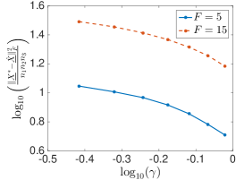
Figure 1: Plot for log per-entry approximation error $\log\left(\frac{\|\hat{\underline{X}}-\underline{X}^{*}\|_{F}^{2}}{n_{1}n_{2}n_{3}}\right)$ vs the log sampling rate: $\log\left(\gamma\right)$ for the two ranks $F=5,15$. The slope at the higher sampling rates is approximately $-1$ (the rate predicted by our theory) in both cases.

VII Conclusion and Future Directions

In this work we extend the statistical theory of complexity-penalized maximum likelihood estimation developed in [8, 18, 19] to noisy tensor completion for tensors admitting CP decomposition with a sparse factor. In particular, we provide theoretical guarantees on the performance of sparsity-regularized maximum likelihood estimation under a Bernoulli sampling assumption and general i.i.d. noise. We then instantiate the general result for the specific case of additive white Gaussian noise. We also provided an ADMM-based algorithmic framework to solve the complexity-penalized maximum likelihood estimation problem and provide numerical experiments to validate the theoretical bounds on synthetic data.

Obtaining error bounds for other noise distributions and non-linear observation setting such 1-bit quantized observations is an interesting possible research direction. Extending the main result to approximately sparse CP factor or to tensors with multiple sparse CP factor are also important directions for future research.

VIII Acknowledgements

We thank Professor Nicholas Sidiropoulos for his insightful guidance and discussions on tensors which helped in completion of this work. Swayambhoo Jain and Jarvis Haupt were supported by the DARPA Young Faculty Award, Grant N66001-14-1-4047. Alexander Gutierrez was supported by the NSF Graduate Research Fellowship Program under Grant No. 00039202.

IX Appendix

IX-A Proof of Main Theorem

The proof of our main result is an application of the following general lemma.

Lemma 1.

Let $\underline{X^{*}}\in\mathbb{R}^{n_{1}\times n_{2}\times n_{3}}$ and let $\mathcal{X}$ be a finite collection of candidate reconstructions with assigned weights $\operatorname{pen}(\underline{X})\geq 1$ satisfying the Kraft-McMillan inequality over $\mathcal{X}$.

$$\sum_{\underline{X}\in\mathcal{X}}2^{-\operatorname{pen}(\underline{X})}\leq 1.$$ (13)

Fix an integer $k\leq m\leq n_{1}n_{2}n_{3}$ and let $\gamma=\frac{m}{n_{1}n_{2}n_{3}}$ and generate $n_{1}n_{2}n_{3}$ i.i.d. Bernoulli$(\gamma)$ random variables $S_{i,j,k}$ so that entry $(i,j,k)\in S$ if $S_{i,j,k}=1$ and $(i,j,k)\notin S$ otherwise. Conditioned on $S$ we obtain independent measurements $Y_{S}\sim p_{X^{*}_{S}}=\prod_{(i,j,k)\in S}p_{X^{*}_{i,j,k}}$. Then if $Q_{D}$ is an upper bound for the maximum KL-divergence

$$Q_{D}\geq\max_{\underline{X}\in\mathcal{X}}\max_{(i,j,k)}D(p_{X^{*}_{i,j,k}}\|p_{X_{i,j,k}}),$$

it follows that for any

$$\xi\geq(1+\frac{2Q_{D}}{3})\cdot 2\log 2$$ (14)

the compexity-penalized maximum likelihood estimator

$$\hat{\underline{X}}^{\xi}(S,\underline{Y}_{S})=\operatorname*{\arg\,\min}_{\underline{X}\in\mathcal{X}}\left\{-\log p_{\underline{X}_{S}}(\underline{Y}_{S})+\xi\operatorname{pen}(\underline{X})\right\}$$

satisfies the error bound

$$\frac{\mathbb{E}_{S,\underline{Y}_{S}}\left[-2\log(A(p_{\hat{X}^{*}},p_{X^{*}}))\right]}{n_{1}n_{2}n_{3}}\leq\frac{8Q_{D}\log m}{m}+$$

$$3\min_{\underline{X}\in\mathcal{X}}\left\{\frac{D(p_{\underline{X}^{*}}\|p_{\underline{X}})}{n_{1}n_{2}n_{3}}+\left(\xi+\frac{4Q_{D}\log 2}{3}\right)\frac{\operatorname{pen}(\underline{X})}{m}\right\}.$$

Proof.

The proof appears in Appendix section IX-B. ∎

For using the result in Lemma 1 we need to define penalties $\operatorname{pen}(\underline{X})\geq 1$ on candidate reconstructions $\underline{X}$ of $\underline{X}^{*}$, so that for every subset $\mathcal{X}$ of the set $\mathcal{X}^{\prime}$ specified in the conditions of Theorem 1 the summability condition $\sum_{\underline{X}\in\mathcal{X}}2^{-\operatorname{pen}(\underline{X})}\leq 1$ holds. To this end, we will use the fact that for any $\mathcal{X}\subseteq\mathcal{X}^{\prime}$ we always have $\sum_{\underline{X}\in\mathcal{X}}2^{-\operatorname{pen}(\underline{X})}\leq\sum_{\underline{X}\in\mathcal{X}^{\prime}}2^{-\operatorname{pen}(\underline{X})}$; thus, it suffices for us to show that for the specific set $\mathcal{X}^{\prime}$ described in (5), the penalty satisfies the Kraft-McMillan inequality:

$$\sum_{\underline{X}\in\mathcal{X}^{\prime}}2^{-\operatorname{pen}(\underline{X})}\leq 1.$$ (15)

The Kraft-Mcmillan Inequality is automatically satisfied if we set the $\operatorname{pen}(\underline{X})$ to be the code length of some uniquely decodable binary code for the elements $\underline{X}\in\mathcal{X}^{\prime}$ [25].

We utilize a common encoding strategy for encoding the elements of $\mathcal{A}$ and $\mathcal{B}$. We encode each entry of the matrices using $\log_{2}(L_{\rm lev})$ bits in this manner the total number of bits needed to code any elements in $\mathcal{A}$ and $\mathcal{B}$ is $n_{1}F\log_{2}(L_{\rm lev})$ and $n_{2}F\log_{2}(L_{\rm lev})$ respectively. Since the elements of set $\mathcal{C}$ are sparse we follow a two step procedure: first we encode the location of the non-zero elements using $\log_{2}L_{\rm loc}$ bits where $L_{\rm loc}=2^{\lceil\log_{2}(n_{3}F)\rceil}$ and then we encode the entry using $\log_{2}(L_{\rm lev})$ bits. Now, we let $\mathcal{X}^{\prime\prime}$ be the set of all such $\underline{X}$ with CPD factors $A\in\mathcal{A}$,$B\in\mathcal{B}$, $C\in\mathcal{C}$, and let the code for each $\underline{X}$ be the concatenation of the (fixed-length) code for $A$ followed by (fixed-length) code for $B$ followed by the (variable-length) code for $C$. It follows that we may assign penalties $\operatorname{pen}(\underline{X})$ to all $\underline{X}\in\mathcal{X}^{\prime\prime}$ whose lengths satisfy

$$\operatorname{pen}(\underline{X})=(n_{1}+n_{2})F\log_{2}L_{\rm lev}+\|C\|_{0}\log_{2}(L_{\rm loc}L_{\rm lev}).$$

By construction such a code is uniquely decodable, since by the Kraft McMillan inequality we have $\sum_{X\in\mathcal{X}^{\prime\prime}}2^{-\operatorname{pen}(\underline{X})}\leq 1$. Further, since $\mathcal{X}^{\prime}\subset\mathcal{X}^{\prime\prime}$ this also satisfies the inequality $\sum_{\underline{X}\in\mathcal{X}}2^{-\operatorname{pen}(\underline{X})}\leq 1$ in (13) in Lemma 1 is satisfied for $\mathcal{X}^{\prime}$ sa defined in statement of the Theorem 1. Now for any set $\underline{X}\subseteq\mathcal{X}^{\prime}$ and using coding strategy described above, the condition (13) in Lemma (1) is satisfied. So for randomly subsampled and noisy observations $Y_{\mathcal{S}}$ our estimates take the form

$$\widehat{\underline{X}}^{\xi} =\underset{\underline{X}=[A,B,C]\in\mathcal{X}}{\textrm{arg min}}\left\{-\log p_{X_{\mathcal{S}}}(Y_{\mathcal{S}})+\xi\operatorname{pen}(\underline{X})\right\}$$

$$=\underset{\underline{X}=[A,B,C]\in\mathcal{X}}{\textrm{arg min}}\left\{-\log p_{X_{\mathcal{S}}}(Y_{\mathcal{S}})+\xi\log_{2}(L_{\rm loc}L_{\rm lev})\|C\|_{0}\right\}$$

Further, when $\xi$ satisfies (14), we have

$$\frac{\mathbb{E}_{S,\underline{Y}_{S}}\left[-2\log(A(p_{\hat{X}^{*}},p_{X^{*}}))\right]}{n_{1}n_{2}n_{3}}\leq\frac{8Q_{D}\log m}{m}+$$

$$3\min_{\underline{X}\in\mathcal{X}}\left\{\frac{D(p_{\underline{X^{*}}}\|p_{\underline{X}})}{n_{1}n_{2}n_{3}}+\left(\xi+\frac{4Q_{D}\log 2}{3}\right)\right.$$

$$\left.\cdot\frac{(n_{1}+n_{2})F\log_{2}L_{\rm lev}+\|C\|_{0}\log_{2}(L_{\rm loc}L_{\rm lev})}{m}\right\}$$

$$\leq\frac{8Q_{D}\log m}{m}+$$

$$3\min_{\underline{X}\in\mathcal{X}}\left\{\frac{D(p_{\underline{X^{*}}}\|p_{\underline{X}})}{n_{1}n_{2}n_{3}}+\left(\xi+\frac{4Q_{D}\log 2}{3}\right)\right.$$

$$\qquad\qquad\left.\cdot\log_{2}(L_{\rm loc}L_{\rm lev})\frac{(n_{1}+n_{2})F+\|C\|_{0}}{m}\right\}.$$

Finally, we let $\lambda=\xi\cdot\log_{2}(L_{\rm loc}L_{\rm lev})$ and using the relation that

$$\log_{2}L_{\rm loc}L_{\rm lev}\leq 2\cdot(\beta+2)\cdot\log(n_{\max})$$ (16)

which follows by our selection of $L_{\rm lev}$ and $L_{\rm loc}$ and the fact that $F,n_{3}\leq n_{\max}$ and $n_{\max}\geq 4$. Using the condition (16) and (14) in Lemma 1 it follows that for

$$\lambda\geq 4(\beta+2)\left(1+\frac{2Q_{D}}{3}\right)\log(n_{\max})$$

the estimate

$$\hat{{\underline{X}}}^{\lambda}=\operatorname*{\arg\,\min}_{\underline{X}=[A,B,C]\in\mathcal{X}}\left(-\log p_{\underline{X}_{S}}(Y_{S})+\lambda\left\|C\right\|_{0}\right),$$ (17)

satisfies the bound (1) in Thereom 1.

IX-B Proof of Lemma

The main requirement for the proof of this lemma is to show that our random Bernoulli measurement model is “good” in the sense that it will allow us to apply some known concentration results. Let $Q_{D}$ be an upper bound on the KL-divergence of $p_{X_{i,j}}$ from $p_{\underline{X}^{*}_{i,j}}$ over all elements $X\in\mathcal{X}$:

$$Q_{D}\geq\max_{\underline{X}\in\mathcal{X}}\max_{i,j}D(p_{\underline{X}^{*}_{i,j,k}}\|p_{\underline{X}_{i,j,k}}).$$

Similarly, let $Q_{A}$ be an upper bound on negative two times the log of the Hellinger affinities between the same:

$$Q_{A}\geq\max_{\underline{X}\in\mathcal{X}}\max_{i,j}-2\log\left(A(p_{\underline{X}^{*}_{i,j,k}}\|p_{\underline{X}_{i,j,k}})\right).$$

Let $m\leq n_{1}n_{2}n_{3}$ be the expected total number of measurements and $\gamma=m/(n_{1}n_{2}n_{3})$ to be the ratio of measured entries to total entries. Given any $\delta\in(0,1)$ define the “good” set $\mathcal{G}_{\gamma,\delta}$ as the subset of all possible sampling sets that satisfy a desired property:

$$\mathcal{G}_{\gamma,\delta}:=\Bigg{\{}S\subseteq[n_{1}]\times[n_{2}]\times[n_{3}]:\left(\bigcap_{\underline{X}\in\mathcal{X}}D(p_{\underline{X}^{*}_{S}}\|p_{\underline{X}_{S}})\leq\frac{3\gamma}{2}D(p_{\underline{X}^{*}}\|p_{\underline{X}})+(4/3)Q_{D}[\log(1/\delta)+\operatorname{pen}(\underline{X})\log 2]\right)$$

$$\cap\left(\bigcap_{\underline{X}\in\mathcal{X}}(-2\log A(p_{\underline{X}^{*}_{S}},p_{\underline{X}_{S}}))\geq\frac{\gamma}{2}(-2\log A(p_{\underline{X}^{*}},p_{\underline{X}}))-(4/3)Q_{A}[\log(1/\delta)+\operatorname{pen}(\underline{X})\log 2]\right)\Bigg{\}}$$

We show that an Erdós-Renyi model with parameter $\gamma$ will be “good” with high probability in the following lemma.

Lemma 2.

Let $\mathcal{X}$ be a finite collection of countable estimates $\underline{X}$ for $\underline{X^{*}}$ with penalties $\operatorname{pen}(\underline{X})$ satifying the Kraft inequality (13). Then for any fixed $\gamma,\delta\in(0,1)$ let $S$ be a random subset of $[n_{1}]\times[n_{2}]\times[n_{3}]$ be a random subset generated according the Erdós-Renyi model.Then $\mathbb{P}[S\notin\mathcal{G}_{\gamma,\delta})\leq 2\delta.$

Proof.

Note that $\mathcal{G}_{\gamma,\delta}$ is defined in terms of an intersection of two events, define them to be

$$\mathcal{E}_{D}:=\left\{\bigcap_{\underline{X}\in\mathcal{X}}D(p_{\underline{X^{*}}_{S}}\|p_{\underline{X}_{S}})\leq\frac{3\gamma}{2}D(p_{\underline{X^{*}}}\|p_{\underline{X}})+(4/3)Q_{D}[\log(1/\delta)+\operatorname{pen}(\underline{X})\log 2]\right\}$$

and

$$\mathcal{E}_{A}:=\left\{\bigcap_{\underline{X}\in\mathcal{X}}(-2\log A(p_{\underline{X^{*}}_{S}},p_{\underline{X}_{S}}))\geq\frac{\gamma}{2}(-2\log A(p_{\underline{X^{*}}},p_{\underline{X}}))-(4/3)Q_{A}[\log(1/\delta)+\operatorname{pen}(\underline{X})\log 2]\right\}.$$

We apply the union bound to find that

$$\mathbb{P}\left[S\notin\mathcal{G}_{\gamma,\delta}\right]\leq\mathbb{P}\left[\mathcal{E}_{u}^{C}\right]+\mathbb{P}\left[\mathcal{E}_{\ell}^{C}\right],$$

and will prove the theorem by showing that each of the two probabilities on the right-hand side are less than $\delta$, starting with $\mathbb{P}[\mathcal{E}_{u}^{C}]$.

Since the observations are conditionally independent given $S$, we know that for fixed $\underline{X}\in\mathcal{X}$,

$$D(p_{\underline{X}_{S}^{*}}\|p_{\underline{X}_{S}})=\sum_{(i,j,k)\in S}D(p_{X^{*}_{i,j,k}}\|p_{X_{i,j,k}})=\sum_{i,j,k}S_{i,j,k}D(p_{X^{*}_{i,j,k}}\|p_{X_{i,j,k}}),$$

where $S_{i,j,k}\stackrel{{\scriptstyle\text{i.i.d.}}}{{\sim}}$Bernoulli($\gamma$). We will show that random sums of this form are concentrated around its mean using the Craig-Bernstein inequality .

The version ofthe Craig-Bernstein inequality that we will use states: let $U_{i,j,k}$ be random variables such that we have the uniform bound $\left|U_{i,j,k}-\mathbb{E}[U_{i,j,k}]\right|\leq\beta$ for all $i,j,k$. Let $\tau>0$ and $\epsilon$ be such that $0<\epsilon\beta/3<1$. Then

$$\mathbb{P}\left[\sum_{i,j,k}(U_{i,j,k}-\mathbb{E}[U_{i,j,k}])\geq\frac{\tau}{\epsilon}+\epsilon\frac{\sum_{i,j,k}\operatorname{var}(U_{i,jk})}{2(1-\epsilon\beta/3)}\right]\leq e^{-\tau}.$$

To apply the Craig-Bernstein inequality to our problem we first fix $\underline{X}\in\mathcal{X}$ and define $U_{i,j,k}=S_{i,j,k}D(p_{\underline{X}^{*}_{i,j,k}}\|p_{X_{i,j,k}})$. Note that $U_{i,j,k}\leq Q_{D}\Rightarrow\left|U_{i,j,k}-\mathbb{E}[U_{i,j,k}]\right|\leq Q_{D}$. We also bound the variance via

$$\operatorname{var}(U_{i,j,k}) =\gamma(1-\gamma)\left(D(p_{X^{*}_{i,j,k}}\|p_{X_{i,j,k}})\right)^{2}$$

$$\leq\gamma\left(D(p_{X^{*}_{i,j,k}}\|p_{X_{i,j,k}})\right)^{2}.$$

Then let $\epsilon=\frac{3}{4Q_{D}}$ and $\beta=Q_{D}$ in (IX-B) to get that

$$\mathbb{P}\left[\sum_{i,j,k}(S_{i,j,k}-\gamma)D(p_{X^{*}_{i,j,k}}\|p_{X_{i,j,k}})\geq\frac{4Q_{D}\tau}{3}+\frac{\sum_{i,j,k}\gamma\cdot\left(D(p_{X^{*}_{i,j,k}}\|p_{X_{i,j,k}})\right)^{2}}{2Q_{D}}\right]\leq e^{-\tau}.$$

Now use the fact that $D(p_{X^{*}_{i,j,k}}\|p_{X_{i,j,k}})\leq Q_{D}$ by definition to cancel out the square term to get:

$$\mathbb{P}\left[\sum_{i,j,k}(S_{i,j,k}-\gamma)D(p_{X^{*}_{i,j,k}}\|p_{X_{i,j,k}})\geq\frac{4Q_{D}\tau}{3}+\frac{3\gamma}{2}\sum_{i,j,k}\cdot D(p_{X^{*}_{i,j,k}}\|p_{X_{i,j,k}})\right]\leq e^{-\tau}.$$

Finally, we define $\delta=e^{-\tau}$, and simplify to arrive at

$$\mathbb{P}\left[D(p_{\underline{X}^{*}_{S}}\|p_{\underline{X}_{S}})\geq\frac{4Q_{D}\log(1/\delta)}{3}+\frac{3\gamma}{2}D(p_{\underline{X}^{*}}\|p_{\underline{X}})\right]\leq\delta,$$ (18)

for any $\delta$.

To get a uniform bound over all $\underline{X}\in\mathcal{X}$ define $\delta_{\underline{X}}:=\delta 2^{-\operatorname{pen}(\underline{X})}$ and use the bound in (18) with $\delta_{\underline{X}}$ and apply the union bound over the class $\mathcal{X}$ to find that

$$\mathbb{P}\left[\bigcup_{\underline{X}\in\mathcal{X}}D(p_{\underline{X}_{S}^{*}}\|p_{\underline{X}_{S}})\geq\frac{3\gamma}{2}D(p_{\underline{X}^{*}}\|p_{\underline{X}})+\frac{4Q_{D}}{3}\left[\log(1/\delta)+\operatorname{pen}(\underline{X})\cdot\log 2\right]\right]\leq\delta.$$ (19)

An similar argument (applying Craig-Bernstein and a union bound) can be applied to $\mathcal{E}_{A}$ to obtain

$$\mathbb{P}\left[\bigcup_{\underline{X}\in\mathcal{X}}\left(-2\log A(p_{\underline{X}_{S}^{*}},p_{\underline{X}_{S}})\right)\leq\frac{\gamma}{2}(-2\log A(p_{\underline{X}^{*}},p_{\underline{X}}))-(4Q_{A}/3)[\log(1/\delta)+\operatorname{pen}(\underline{X})\cdot\log 2]\right]\leq\delta$$ (20)

This completes the proof of lemma 2. ∎

Given lemma 2, the rest of the proof of lemma 1 is a straightforward extension of the already-published proof of lemma A.1 in [8].

IX-C Proof of Corollary 1

We first establish a general error bound, which we then specialize to the case stated in the corollary. Note that for $\underline{X}^{*}$ as specified and any $\underline{X}\in\mathcal{X}$, using the model (8) we have

$$D(p_{X_{i,j,k}^{*}}\|p_{X_{i,j,k}})=\frac{(X_{i,j,k}^{*}-X_{i,j,k})^{2}}{2\sigma^{2}}$$

for any fixed $(i,j,k)\in S$. It follows that $D(p_{\underline{X}^{*}}\|p_{\underline{X}})=\|\underline{X}^{*}-\underline{X}\|_{F}^{2}/2\sigma^{2}$. Further. as the amplitudes of entries of $\underline{X}^{*}$ and all $\underline{X}\in\mathcal{X}$ upper bounded by $X_{\max}$, it is easy to see that we may choose $Q_{D}=2X_{\max}^{2}/\sigma^{2}$. Also, for any $\underline{X}\in\mathcal{X}$ and any fixed $(i,j,k)\in S$ it is easy to show that in this case

$$-2\log A(p_{X_{i,j,k}},p_{X_{i,j,k}^{*}})=\frac{(X_{i,j,k}^{*}-X_{i,j,k})^{2}}{4\sigma^{2}},$$

so that $-2\log A(p_{\underline{X}},p_{\underline{X}^{*}})=\|\underline{X}^{*}-\underline{X}\|_{F}^{2}/4\sigma^{2}$. It follows that

$$\mathbb{E}_{S,\underline{Y}_{S}}\left[-2\log A(p_{\hat{\underline{X}}},p_{\underline{X}^{*}})\right]=\frac{\mathbb{E}_{S,\underline{Y}_{S}}\left[\|\underline{X}^{*}-\widehat{\underline{X}}\|_{F}^{2}\right]}{4\sigma^{2}}.$$

Now for using Theorem 1, we first substitute the value of $Q_{D}=2X_{\max}^{2}/\sigma^{2}$ to obtain the following condition on $\lambda$

$$\lambda\geq 4\cdot\left(1+\frac{4X_{\max}^{2}}{3\sigma^{2}}\right)\cdot(\beta+2)\cdot\log(n_{\max}).$$

Above condition implies that the specific choice of $\lambda$ given (10) is a valid choice to use if we want to invoke Theorem 1. So fixing $\lambda$ as given (10) and using Theorem 1, the sparsity penalized ML estimate satisfies the per-element mean-square error bound

$$\frac{\mathbb{E}_{S,\underline{Y}_{S}}\left[\|\underline{X}^{*}-\widehat{\underline{X}}\|_{F}^{2}\right]}{n_{1}n_{2}n_{3}}\leq \frac{64X_{\max}^{2}\log m}{m}+$$

$$6\cdot\min_{\underline{X}\in\mathcal{X}}\left\{\frac{\|\underline{X}^{*}-\underline{X}\|_{F}^{2}}{n_{1}n_{2}n_{3}}+\left(2\sigma^{2}\lambda+\frac{24X_{\max}^{2}(\beta+2)\log(n_{\max})}{3}\right)\left(\frac{(n_{1}+n_{2})F+\|C\|_{0}}{m}\right)\right\}.$$

Notice that the above inequality is sort of an oracle type inequality because it implies that for any $\underline{X}\in\mathcal{X}$ we have

$$\frac{\mathbb{E}_{S,\underline{Y}_{S}}\left[\|\underline{X}^{*}-\widehat{\underline{X}}\|_{F}^{2}\right]}{n_{1}n_{2}n_{3}}\leq \frac{64X_{\max}^{2}\log m}{m}+$$

$$6\cdot\left\{\frac{\|\underline{X}^{*}-\underline{X}\|_{F}^{2}}{n_{1}n_{2}n_{3}}+\left(2\sigma^{2}\lambda+\frac{24X_{\max}^{2}(\beta+2)\log(n_{\max})}{3}\right)\left(\frac{(n_{1}+n_{2})F+\|C\|_{0}}{m}\right)\right\}.$$

We use this inequality for a specific candidate reconstruction of the form $\underline{X}^{*}_{Q}=[A^{*}_{Q},B^{*}_{Q},C^{*}_{Q}]$ where the entries of s $A^{*}_{Q}$ are the closest discretized surrogates of the entries of $A^{*}$, $B^{*}_{Q}$ are the closest discretized surrogates of the entries of $B^{*}$, and $C^{*}_{Q}$ are the closest discretized surrogates of the non-zeros entries of $C^{*}$ (and zero otherwise). For proceeding further we need to bound $\|\underline{X}_{Q}^{*}-\underline{X}^{*}\|_{\max}$. For this purpose we consider matricization of tensor across the third dimension as follows

$$\|\underline{X}_{Q}^{*}-\underline{X}^{*}\|_{\max} =\left\|\left(B_{Q}^{*}\odot A_{Q}^{*}\right)(C^{*}_{Q})^{T}-\left(B^{*}\odot A^{*}\right)(C^{*})^{T}\right\|_{\max}$$

Next we write $A_{Q}^{*}=A^{*}+\Delta_{A}$, $B_{Q}^{*}=B^{*}+\Delta_{B}$ and $C_{Q}^{*}=C^{*}+\Delta_{C}$ with straight forward matrix multiplication we can obtain that

$$\left(B_{Q}^{*}\odot A_{Q}^{*}\right)(C^{*}_{Q})^{T}= \left(B^{*}\odot A^{*}\right)(C^{*})^{T}+\left(\Delta_{A}\odot B^{*}+A^{*}\odot\Delta_{B}+\Delta_{A}\odot\Delta_{B}\right)(C^{*})^{T}$$

$$+\left(A^{*}\odot B^{*}+\Delta_{A}\odot B^{*}+A^{*}\odot\Delta_{B}+\Delta_{A}\odot\Delta_{B}\right)\Delta_{C}^{T}$$ (21)

Using this identity it follows

$$\|\underline{X}_{Q}^{*}-\underline{X}^{*}\|_{\max}=\left\|\left(\Delta_{A}\odot B^{*}+A^{*}\odot\Delta_{B}+\Delta_{A}\odot\Delta_{B}\right)(C^{*})^{T}+\left(A^{*}\odot B^{*}+\Delta_{A}\odot B^{*}+A^{*}\odot\Delta_{B}+\Delta_{A}\odot\Delta_{B}\right)\Delta_{C}^{T}\right\|_{\max}$$

Now using the facts that $\|A\odot B\|_{\max}=\|A\|_{\max}\|B\|_{\max}$, $\|AB\|_{\max}\leq F\|A\|\|B\|_{\max}$ and triangle inequality for the $\|\cdot\|_{\max}$ norm it is easy to show that

$$\|\underline{X}_{Q}^{*}-\underline{X}^{*}\|_{\max}\leq F\left[(\|\Delta_{A}\|_{\max}+\|A\|_{\max})(\|\Delta_{B}\|_{\max}+\|B\|_{\max})(\|\Delta_{C}\|_{\max}+\|C\|_{\max})-\|A\|_{\max}\|B\|_{\max}\|C\|_{\max}\right]$$

Further, using the fact that $\|\Delta_{A}\|_{\max}\leq\frac{A_{\max}}{L_{\rm lev}-1}$ , $\|\Delta_{B}\|_{\max}\leq\frac{B_{\max}}{L_{\rm lev}-1}$, and $\|\Delta_{C}\|_{\max}\leq\frac{C_{\max}}{L_{\rm lev}-1}$, we have

$$\|\underline{X}_{Q}^{*}-\underline{X}^{*}\|_{\max}$$

$$\leq F\left[\left(\frac{A_{\max}}{L_{\rm lev}-1}+A_{\max}\right)\left(\frac{B_{\max}}{L_{\rm lev}-1}+\|B\|_{\max}\right)\left(\frac{C_{\max}}{L_{\rm lev}-1}+C_{\max}\right)-A_{\max}B_{\max}C_{\max}\right]$$

$$\leq FA_{\max}B_{\max}C_{\max}\left[\left(1+\frac{1}{L_{\rm lev}-1}\right)^{3}-1\right]$$

$$\leq\frac{FA_{\max}B_{\max}C_{\max}}{L_{\rm lev}-1}\left[3+\frac{3}{L_{\rm lev}-1}+\frac{1}{(L_{\rm lev}-1)^{2}}\right]$$

$$\leq\frac{7FA_{\max}B_{\max}C_{\max}}{L_{\rm lev}-1},$$

where in the second last step we have used $L_{\rm lev}\geq 2$. Now, it is straight-forward to show that our choice of $\beta$ in (9) implies $L_{\rm lev}\geq 14FA_{\max}B_{\max}C_{\max}/X_{\max}+1$, so each entry of $\|\underline{X}_{Q}^{*}-\underline{X}^{*}\|_{\max}\leq X_{\max}/2$. This further implies that for the candidate estimate $\underline{X}_{Q}^{*}$ we have $\|\underline{X}_{Q}^{*}\|_{\max}\leq X_{\max}$, i.e., $\underline{X}_{Q}^{*}\in\mathcal{X}$. Moreover, we

$$\frac{\|\underline{X}^{*}-\underline{X}^{*}_{Q}\|_{F}^{2}}{n_{1}n_{2}n_{3}}\leq\left(\frac{7FA_{\max}B_{\max}C_{\max}}{L_{\rm lev}-1}\right)^{2}\leq\frac{X_{\max}^{2}}{m},$$ (22)

where the last inequality follows from the fact that our specific choice of $\beta$ in (9) also implies $L_{\rm lev}\geq 7F\sqrt{m}A_{\max}B_{\max}C_{\max}/X_{\max}$.

Finally, we evaluate the oracle inequality for (IX-C) for $\underline{X}_{Q}^{*}$ and using the fact that $\|C^{*}_{Q}\|_{0}=\|C^{*}\|_{0}$ and using the value of $\lambda$ specified in the corollary we have

$$\frac{\mathbb{E}_{S,\underline{Y}_{S}}\left[\|\underline{X}^{*}-\widehat{\underline{X}}\|_{F}^{2}\right]}{n_{1}n_{2}n_{3}}\leq\frac{70X_{\max}^{2}\log m}{m}+24(\sigma^{2}+2X_{\max}^{2})(\beta+2)\log(n_{\max})\left(\frac{(n_{1}+n_{2})F+\|C^{*}\|_{0}}{m}\right).$$

References

• [1] Leslie Hogben, “Graph theoretic methods for matrix completion problems,” Linear Algebra and Its Applications, vol. 328, no. 1-3, pp. 161–202, 2001.
• [2] Raghunandan Keshavan, Andrea Montanari, and Sewoong Oh, “Matrix completion from noisy entries,” in Advances in Neural Information Processing Systems, 2009, pp. 952–960.
• [3] Emmanuel J Candes and Yaniv Plan, “Matrix completion with noise,” Proceedings of the IEEE, vol. 98, no. 6, pp. 925–936, 2010.
• [4] Emmanuel J Candès and Terence Tao, “The power of convex relaxation: Near-optimal matrix completion,” IEEE Transactions on Information Theory, vol. 56, no. 5, pp. 2053–2080, 2010.
• [5] Benjamin Recht, “A simpler approach to matrix completion,” The Journal of Machine Learning Research, vol. 12, pp. 3413–3430, 2011.
• [6] Prateek Jain, Praneeth Netrapalli, and Sujay Sanghavi, “Low-rank matrix completion using alternating minimization,” in Proceedings of the forty-fifth annual ACM symposium on Theory of computing. ACM, 2013, pp. 665–674.
• [7] Akshay Soni, Swayambhoo Jain, Jarvis Haupt, and Stefano Gonella, “Error bounds for maximum likelihood matrix completion under sparse factor models,” in Signal and Information Processing (GlobalSIP), 2014 IEEE Global Conference on. IEEE, 2014, pp. 399–403.
• [8] Akshay Soni, Swayambhoo Jain, Jarvis Haupt, and Stefano Gonella, “Noisy matrix completion under sparse factor models,” IEEE Transactions on Information Theory, vol. 62, no. 6, pp. 3636–3661, June 2016.
• [9] Tamara G Kolda and Brett W Bader, “Tensor decompositions and applications,” SIAM review, vol. 51, no. 3, pp. 455–500, 2009.
• [10] Nicholas D Sidiropoulos, Lieven De Lathauwer, Xiao Fu, Kejun Huang, Evangelos E Papalexakis, and Christos Faloutsos, “Tensor decomposition for signal processing and machine learning,” arXiv preprint arXiv:1607.01668, 2016.
• [11] Liang Xiong, Xi Chen, Tzu-Kuo Huang, Jeff G Schneider, and Jaime G Carbonell, “Temporal collaborative filtering with Bayesian probabilistic tensor factorization.,” in SDM. SIAM, 2010, vol. 10, pp. 211–222.
• [12] Kejun Huang, Nicholas D Sidiropoulos, and Athanasios P Liavas, “A flexible and efficient algorithmic framework for constrained matrix and tensor factorization,” IEEE Transactions on Signal Processing, vol. 64, no. 19, pp. 5052–5065, 2016.
• [13] Weiwei Shi, Yongxin Zhu, S Yu Philip, Mengyun Liu, Guoxing Wang, Zhiliang Qian, and Yong Lian, “Incomplete electrocardiogram time series prediction,” in Biomedical Circuits and Systems Conference (BioCAS), 2016 IEEE. IEEE, 2016, pp. 200–203.
• [14] Genevera Allen, “Sparse higher-order principal components analysis.,” in AISTATS, 2012, vol. 15.
• [15] Roland Ruiters and Reinhard Klein, “BTF compression via sparse tensor decomposition,” in Computer Graphics Forum. Wiley Online Library, 2009, vol. 28, pp. 1181–1188.
• [16] Evangelos E Papalexakis, Nicholas D Sidiropoulos, and Rasmus Bro, “From k-means to higher-way co-clustering: Multilinear decomposition with sparse latent factors,” IEEE transactions on signal processing, vol. 61, no. 2, pp. 493–506, 2013.
• [17] Yanwei Pang, Zhao Ma, Jing Pan, and Yuan Yuan, “Robust sparse tensor decomposition by probabilistic latent semantic analysis,” in Image and Graphics (ICIG), 2011 Sixth International Conference on. IEEE, 2011, pp. 893–896.
• [18] Eric D Kolaczyk and Robert D Nowak, “Multiscale likelihood analysis and complexity penalized estimation,” Annals of statistics, pp. 500–527, 2004.
• [19] Jonathan Q Li and Andrew R Barron, “Mixture density estimation,” in Advances in Neural Information Processing Systems 12. Citeseer, 1999.
• [20] Ming Yuan and Cun-Hui Zhang, “On tensor completion via nuclear norm minimization,” Foundations of Computational Mathematics, vol. 16, no. 4, pp. 1031–1068, 2016.
• [21] Ji Liu, Przemyslaw Musialski, Peter Wonka, and Jieping Ye, “Tensor completion for estimating missing values in visual data,” IEEE Transactions on Pattern Analysis and Machine Intelligence, vol. 35, no. 1, pp. 208–220, 2013.
• [22] Bo Huang, Cun Mu, Donald Goldfarb, and John Wright, “Provable low-rank tensor recovery,” Optimization-Online, vol. 4252, pp. 2, 2014.
• [23] Yangyang Xu, Ruru Hao, Wotao Yin, and Zhixun Su, “Parallel matrix factorization for low-rank tensor completion,” arXiv preprint arXiv:1312.1254, 2013.
• [24] Prateek Jain and Sewoong Oh, “Provable tensor factorization with missing data,” in Advances in Neural Information Processing Systems, 2014, pp. 1431–1439.
• [25] Thomas M Cover and Joy A Thomas, Elements of information theory, John Wiley & Sons, 2012.