Kinetic approach to relativistic dissipation

Abstract

Despite a long record of intense efforts, the basic mechanisms by which dissipation emerges from the microscopic dynamics of a relativistic fluid still elude a complete understanding. In particular, several details must still be finalized in the pathway from kinetic theory to hydrodynamics mainly in the derivation of the values of the transport coefficients. In this Letter, we approach the problem by matching data from lattice kinetic simulations with analytical predictions. Our numerical results provide neat evidence in favour of the Chapman-Enskog procedure, as suggested by recently theoretical analyses, along with qualitative hints at the basic reasons why the Chapman-Enskog expansion might be better suited than Grad’s method to capture the emergence of dissipative effects in relativistic fluids.

The basic mechanisms by which dissipative effects emerge from the microscopic dynamics of relativistic fluids remains are still not fully understood in relativistic hydrodynamics. It has been long-recognized that the parabolic nature of the Laplace operator is inconsistent with relativistic invariance, as it implies superluminal propagation, hence non-causal and unstable behavior Hiscock and Lindblom (1983, 1985, 1987). This can be corrected by resorting to fully-hyperbolic formulations of relativistic hydrodynamics, whereby space and time come on the same first-order footing, but the exact form of the resulting equations is not uniquely fixed by macroscopic symmetry arguments and thus remains open to debate.

A more fundamental approach is to derive relativistic hydrodynamics from the underlying kinetic theory De Groot (1980), exploiting the advantages of the bottom-up approach: irreversibility is encoded within a local H-theorem Cercignani and Kremer (2002), while dissipation results as an emergent manifestation of weak departure from local equilibrium (low Knudsen-number assumption) and the consequent enslaving of the fast modes to the slow hydrodynamic ones, associated with microscopic conservation laws. At no point does this scenario involve second order derivatives in space, thus preserving relativistic invariance by construction.

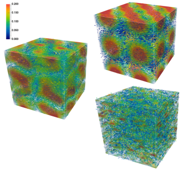
Figure 1: Three-dimensional Taylor-Green vortex configuration of a viscous relativistic fluid, with $\zeta=0$ and $\tau=0.51$ (symbols defined in the text). Top: initial configuration; Middle: later stage in which the vortex configuration becomes unstable; Bottom: final disordered state. Colours code vorticity and arrows represent the velocity field.

In non-relativistic regimes, Grad’s moments method Grad (1949) and the Chapman-Enskog (CE) Chapman and Cowling (1970) approach manage to connect kinetic theory and hydrodynamics in a consistent way, i.e. they provide the same transport coefficients. However, the relativistic regime presents a more controversial picture. The Israel and Stewards (IS) formulation Israel (1976); Israel and Stewart (1979), extending Grad’s method, derives causal and stable equations of motion, at least for hydrodynamics regimes Romatschke (2010). While many earlier works have relied on IS, recent developments have highlighted theoretical shortcomings Denicol et al. (2012) and poor agreement with numerical solutions of the Boltzmann equation Huovinen and Molnar (2009); Bouras et al. (2010).

Recently, several authors have developed new attempts to derive consistent relativistic dissipative hydrodynamics equations. Attempting to circumvent the drawbacks of the IS formulation, Denicol et al. Denicol et al. (2010, 2012); Molnár et al. (2014) have proposed an extension of the moments methods in which the resulting equations of motion are derived directly from the Boltzmann equation and truncated by a systematic power-counting scheme in Knudsen number.

This, in turn, offers the possibility to include a larger number of moments (with respect to the 14 used in the IS formulation), improving the expressions for the transport coefficients. Starting from similar considerations, Jaiswal et al. Jaiswal et al. (2013) have included entropic arguments within Grad’s method and derived relativistic dissipative hydrodynamics equations which take the same form as IS, although with different expressions for the transport coefficients. When compared to IS, these developments lead to solutions closer to the Boltzmann equation and, at least in the ultra-relativistic limit (defined by $\zeta\rightarrow 0$, where $\zeta=mc^{2}/K_{B}~{}T$ is the ratio of particle rest energy and temperature), they yield transport coefficients in good agreement with those calculated via the CE expansion. Interestingly, the CE method itself remains somewhat less explored Jaiswal (2013a, b), with relativistic extensions mostly restricted to the relaxation time approximation. More recently, a novel approach, introduced in a series of works by Tsumura et al. Tsumura and Kunihiro (2012); Tsumura et al. (2015); Kikuchi et al. (2015, 2016), applies renormalization group techniques to the Boltzmann equation. Once again, expressions for bulk (shear) viscosity and heat conductivity coincide with those provided by the CE method. Summing up, the present and somewhat not fully conclusive state of affairs, is that different theoretical approaches, based on different, if not conflicting assumptions, seem to converge towards the results provided by the CE approach. Conceptual shortcomings of the moments method, recently highlighted also in the non-relativistic framework Velasco et al. (2002); Struchtrup and Torrilhon (2003); Öttinger (2010); Torrilhon (2016), revolve around the use of second-order spatial derivatives in constitutive hydrodynamical equations Tsumura and Kunihiro (2012). On the other hand, objections to the relativistic Chapman-Enskog expansion point to its link to relativistic Navier-Stokes equations, which suffer of basic problems, such as broken causality and resulting instabilities Denicol et al. (2010, 2012). In a less than crystal-clear situation, one would like to validate theory towards experimental data, but a controlled experimental setup is not a viable option at this point in time. Given the circumstances, numerical simulation stands up as a very precious alternative to gain new insights into this problem.

Recent works Florkowski et al. (2013); Bhalerao et al. (2014) have presented 1D simulations of the (ultra)-relativistic Boltzmann equation in the relaxation time approximation, showing results asymptotically compatible with the CE approach. This letter follows a similar line and reports the results of lattice-kinetic simulations of a relativistic flow in a controlled setup for which an approximate analytical hydrodynamic solution can be derived. We match analytical and numerical results in order to study the dependence of hydrodynamic transport coefficients on parameters defined at the mesoscale. To this purpose, we study the time evolution of a Taylor-Green vortex configuration in two and three spatial dimensions (see Figure 1) and probe the functional dependence of the transport coefficients on $\zeta$, extending previous work confined to the $\zeta\to 0$ limit. Our main result is a neat indication that CE predictions accurately match numerical data, and they do so over a remarkably wide $\zeta$ range, starting from the ultra-relativistic regime and seamlessly going over to the well-known non relativistic case. Our simulations use a recently developed relativistic lattice Boltzmann model (RLBM) Gabbana et al. (2017), able to handle massive particles, providing, to the best of our knowledge, the first analysis of dissipative effects for relativistic, but not-necessarily ultra-relativistic, flows.

In relativistic fluid dynamics, ideal non-degenerate fluids are described by the particle four-flow and energy momentum tensors, which at equilibrium read:

$$N^{\alpha}_{E}= ~{}nU^{\alpha}\quad,$$ (1)

$$T^{\alpha\beta}_{E}= ~{}(P+\epsilon)U^{\alpha}U^{\beta}-Pg^{\alpha\beta}\quad,$$ (2)

where $U^{\alpha}=\gamma~{}(1,\bm{u})$ is the fluid four velocity, ( $\bm{u}$ is the fluid velocity, $\gamma=1/\sqrt{1-u^{2}}$; we use natural units such that $c=1,~{}K_{B}=1$), $P$ the hydrostatic pressure, and $\epsilon$ ($n$) energy (particle) density. We take into account dissipative effects with the Landau-Lifshitz decomposition Cercignani and Kremer (2002):

$$N^{\alpha} =N^{\alpha}_{E}-\frac{n}{P+\epsilon}q^{\alpha}\quad\quad,$$ (3)

$$T^{\alpha\beta} =T^{\alpha\beta}_{E}+P^{<\alpha\beta>}-\varpi\left(g^{\alpha\beta}-U^{\alpha}U^{\beta}\right)\quad,$$ (4)

with:

$$\begin{array}[]{rcrl}q^{\alpha}&=&\lambda&\left(\nabla^{\alpha}T-TU^{\alpha}\partial_{\beta}U^{\beta}\right)\quad,\\ P^{<\alpha\beta>}&=&\eta&\left(\Delta^{\alpha}_{\gamma}\Delta^{\beta}_{\delta}+\Delta^{\alpha}_{\delta}\Delta^{\beta}_{\gamma}-\frac{2}{3}\Delta^{\alpha\beta}\Delta_{\gamma\delta}\right)\nabla^{\gamma}U^{\delta}\quad,\\ \varpi&=&-\mu&\nabla_{\alpha}U^{\alpha}\quad;\end{array}$$

$q^{\alpha}$ is the heat flux, $P^{<\alpha\beta>}$ the pressure deviator, $\varpi$ dynamic pressure, $\lambda$ heat conductivity, and $\eta$ and $\mu$ shear and bulk viscosities, respectively. Further we have:

$$\begin{array}[]{lcl}\nabla^{\alpha}&=&\Delta^{\alpha\beta}\partial_{\beta}\quad,\\ \Delta^{\alpha\beta}&=&g^{\alpha\beta}-U^{\alpha}U^{\beta}\quad,\\ \Delta^{\alpha}_{\beta}&=&\Delta^{\alpha\gamma}\Delta_{\gamma\beta}\quad.\\ \end{array}$$

A kinetic formulation, on the other hand, describes the fluid as a system of interacting particles of rest mass $m$; the particle distribution function $f(x^{\alpha},p^{\beta})$ depends on space-time coordinates $x^{\alpha}=\left(t,\bm{x}\right)$ and momenta $p^{\alpha}=\left(p^{0},\bm{p}\right)=\left(\sqrt{\bm{p}^{2}+m^{2}},\bm{p}\right)$; $f(\bm{x},t,\bm{p})\mathop{}\!\mathrm{d}\bm{x}\mathop{}\!\mathrm{d}\bm{p}$ counts the number of particles in the corresponding volume element in phase space.

The system evolves according to the Boltzmann equation, which, in the absence of external forces, reads as follows:

$$p^{\alpha}\frac{\partial f}{\partial x^{\alpha}}=\Omega(f)\quad.$$ (5)

The collision term $\Omega(f)$ is often replaced by simplified models. For instance, the Anderson-Witting model Anderson and Witting (1974) (a relativistic extension of the well known Bhatnagar-Gross-Krook Bhatnagar et al. (1954) formulation), compatible with the Landau-Lifshitz decomposition, reads

$$\Omega=\frac{p^{\mu}U_{\mu}}{\tau}\left(f-f^{eq}\right)\quad.$$ (6)

The equilibrium distribution $f^{eq}$, following Boltzmann statistics, has been derived many decades ago by Jüttner Jüttner (1911),

$$f^{eq}\simeq e^{-p^{\mu}U_{\mu}/T}\quad.$$ (7)

The Anderson-Witting model has just one parameter, the equilibration (proper-)time $\tau$ and obeys the conservation equations:

$$\partial_{\alpha}N^{\alpha} =0\quad,$$ (8)

$$\partial_{\beta}T^{\alpha\beta} =0\quad.$$ (9)

As discussed in previous paragraphs, a predictive bridge between kinetic theory and hydrodynamics must provide the macroscopic transport coefficients $\lambda,\mu,\eta$, from the mesoscopic ones ($\tau$ in the Anderson-Witting model). Our attempt at contributing further understanding of the issue is based on the following analysis; we: i) consider a relativistic flow for which we are able to compute an approximate hydrodynamical solution depending on the transport coefficients; ii) study the same flow numerically with a lattice Boltzmann kinetic algorithm, obtaining a numerical calibration of the functional relation between the transport coefficients and $\tau$; iii) obtain clear-cut evidence that the CE method successfully matches the numerical results and, iv) double-check our approach using the calibrations obtained in ii) for a numerical study of a different relativistic flow, successfully comparing with other numerical data obtained by different methods.

We consider Taylor-Green vortices Taylor and Green (1937), a well known example of a non-relativistic decaying flow featuring an exact solution of the Navier-Stokes equations, and derive an approximate solution in the mildly relativistic regime. In the non-relativistic case, from the following initial conditions in a 2D periodic domain:

$$u_{x}(x,y,0) = v_{0}\cos{\left(x\right)}\sin{\left(y\right)}$$ , (10)

$$u_{y}(x,y,0) = -v_{0}\cos{\left(y\right)}\sin{\left(x\right)} ,\quad x,y\in[0,2\pi]$$

the solution is given by

$$u_{x}(x,y,t) = v_{0}\cos{\left(x\right)}\sin{\left(y\right)}F(t)$$ , (11)

$$u_{y}(x,y,t) = -v_{0}\cos{\left(y\right)}\sin{\left(x\right)}F(t) ,\quad x,y\in[0,2\pi]$$

with

$$F(t)=\exp{\left(-2\nu~{}t\right)}\quad,$$ (12)

where $\nu$ is the kinematic viscosity of the fluid.

In the relativistic case, we need to solve the conservation equations (Equation 8, Equation 9). We consider a system with a constant initial particle density, and assume that density remains constant. We will verify later this assumption against our numerical results showing that density fluctuations in time are very small. In this case Equation 8 is directly satisfied and the expression of the second order tensor slightly simplifies, since $\nabla_{\alpha}U^{\alpha}=0$. Consequently we drop the term depending on bulk viscosity and rewrite the second order tensor as:

$$T^{\alpha\beta}=-Pg^{\alpha\beta}+(\epsilon+P)U^{\alpha}U^{\beta}+P^{<\alpha\beta>}\quad.$$ (13)

We consider the same initial conditions as in Equation 10, and look for a a solution in the form of Equation 11, with an appropriate function $F_{R}(t)$ replacing $F(t)$. We plug Equation 11 in Equation 13 and derive bulky analytic expressions for the derivatives of the second order tensor. A linear expansion of these expressions in terms of $v_{0}$ yields a much simpler expression for $\partial_{\beta}T^{\alpha\beta}$, leading to the differential equation

$$2\eta F_{R}(t)+(P+\epsilon)F_{R}^{{}^{\prime}}(t)=0\quad.$$ (14)

Assuming $P+\epsilon$ constant, for a fixed value of $\zeta$, we derive an explicit solution:

$$F_{R}(t)=\exp{\left(-\frac{2\eta}{P+\epsilon}t\right)}F_{R}(0)\quad,$$ (15)

depending on just one transport coefficient, the shear viscosity $\eta$. Observe that while the quantity $P+\epsilon$ exhibits some time variation (as found in the simulations) due to the evolution of the local temperature, such fluctuations were found to be negligible.

Next, we compare this analytical solution with data obtained via our LB numerical simulation, aiming at linking $\eta$ to the relaxation time $\tau$. We perform several simulations with different values of the initial speed $v_{0}$ and the mesoscopic parameters, $\tau$ and $\zeta$. We consider small (yet, non negligible) values of $u$ and a very broad range of $\zeta$ values, smoothly bridging between ultra-relativistic to near non-relativistic regimes. To this end, it is expedient to introduce the observable $\bar{u}$:

$$\bar{u}^{2}=\int\int\left(u_{x}^{2}+u_{y}^{2}\right)\mathop{}\!\mathrm{d}x\mathop{}\!\mathrm{d}y\quad,$$ (16)

defined to be proportional to $F_{R}(t)$. Figure 2 gives an example of our numerical results, showing the time evolution of $\bar{u}$, clearly exhibiting an exponential decay.

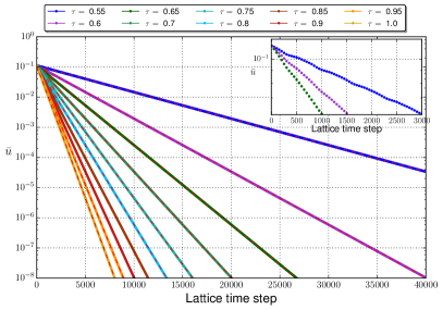
Figure 2: Simulated time evolution of $\bar{u}$ for selected $\tau$ values on a $L=400$ square lattice ($\zeta=0$, $v_{0}=0.2$, $n_{0}=1$, $T_{0}=1$). Lines are fits to the exponential decay predicted by Equation 15. The inset shows non-linear effects in the early phases of the flow.

For each set of mesoscopic values, we perform a linear fit of $\log(\bar{u})$ extracting a corresponding value for $\eta$ via Equation 15. We next assume a dependence of $\eta$ on the mesoscopic parameters, which, on dimensional grounds, reads as

$$\eta=k~{}f\left(\zeta\right)~{}P~{}(\tau-\frac{1}{2})\quad,$$ (17)

with $f(\zeta)$ normalized such that $f(0)=1$. The numerical value of $k$ and the functional form of $f(\zeta)$ contain the physical information on the relation between kinetic and hydrodynamics coefficients. For instance, CE predicts $k=4/5$ and an expression for $f(\zeta)$ to which we shall return shortly; for comparison, Grad’s method predicts $k=2/3$ and a different functional dependence on $\zeta$. We are now able to test that Equation 17 holds correctly, checking that all measurements of $\eta(\tau)$ at a fixed value of $\zeta$ yield a constant value for $k~{}f(\zeta)$.

	$k~{}f(\zeta)$
$\tau$	$\zeta$ = 0	$\zeta$ = 1.6	$\zeta$ = 2	$\zeta$ = 3	$\zeta$ = 4	$\zeta$ = 5	$\zeta$ = 10
0.600	0.8003	0.8319	0.8448	0.8587	0.8892	0.8994	0.9311
0.700	0.8002	0.8318	0.8447	0.8584	0.8888	0.8990	0.9302
0.800	0.8002	0.8318	0.8447	0.8583	0.8887	0.8989	0.9300
0.900	0.8002	0.8318	0.8447	0.8583	0.8887	0.8988	0.9299
1.000	0.8002	0.8317	0.8446	0.8582	0.8887	0.8988	0.9299

Table 1: Fitted values of $k~{}f(\zeta)$ for selected values of $\tau$ and $\zeta$. Statistical errors are smaller than $1$ in the last displayed digit.

One immediately sees from the second column of Table 1 that $k=4/5$ to very high accuracy, consistently with previous results Denicol et al. (2012); Tsumura and Kunihiro (2012); Florkowski et al. (2013); Chattopadhyay et al. (2015). More interesting is the assessment of the functional behavior of $f(\zeta)$. The CE expansion predicts Cercignani and Kremer (2002)

$$f(\zeta)=\frac{\zeta^{3}}{12}\left(\frac{3}{\zeta^{2}}\frac{K_{3}(\zeta)}{K_{2}(\zeta)}-\frac{1}{\zeta}+\frac{K_{1}(\zeta)}{K_{2}(\zeta)}-\frac{Ki_{1}}{K_{2}(\zeta)}\right)\quad,$$ (18)

with $Ki_{1}=\int_{0}^{\infty}e^{-\zeta\cosh(t)}/\cosh(t)\textit{dt}$.

Our numerical findings for $k~{}f(\zeta)$ are shown in Figure 3; For some $\zeta$ values we have used several different quadratures for our LB method (see Ref. Gabbana et al. (2017)), the corresponding results differing from each other by approximately $1\%$; we consider this an estimate of our systematic errors. Figure 3 also shows the CE prediction (Equation 18) that almost perfectly matches our results (we remark that no free parameters are involved in this comparison) and nicely goes over to the well-known non-relativistic limit for large values of $\zeta$. For a more quantitative appreciation of the significance of our result, we also plot the predictions of Grad’s method, which obey the following equation:

$$f(\zeta)=\frac{3}{2}\frac{K_{3}^{2}(\zeta)}{K_{2}(\zeta)~{}K_{4}(\zeta)}\quad.$$ (19)

Comparison of the two curves allows to conclude that our level of resolution is adequate to discriminate between the two options.

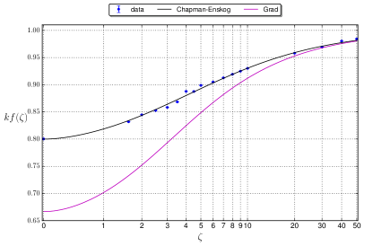
Figure 3: Measured value $k~{}f(\zeta)$ as a function of $\zeta$. The black (magenta) lines are analytic results of the Chapman Enskog (Grad’s) methods for the relativistic Boltzmann equation. To improve resolution at small $\zeta$ values, we map $\zeta\rightarrow\log{(\zeta+\sqrt{1+{\zeta}^{2}})}$ on the x-axis.

We performed the same procedure for fully three dimensional simulations, and the corresponding results hold similar degree of accuracy; details will be presented in an expanded version of this Letter.

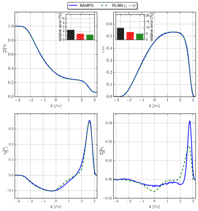
Figure 4: Comparison of BAMPS and our RLBM for the Riemann problem at $t=3.2~{}fm$ ($\zeta=0,\eta/s=0.1$). Top: left) pressure profile; right) velocity profile. Error bars are the L2-difference between BAMPS and RLBM using Grad L=1600 (black), Chapman Enskog L=1600 (red), Chapman Enskog L=12800 (green). Bottom: left) viscous pressure tensor; right) heat flux profile.

Finally, in order to provide a further test of the robustness of our calibration procedure, we consider a significantly different problem, we simulate a 1D shock tube problem in the ultra-relativistic regime ($\zeta=0$), comparing with BAMPS Xu and Greiner (2005), a Monte Carlo numerical solver for the full Boltzmann equation. This simulation uses a $1\times 1\times LZ$ lattice and keeps the ratio $\eta/s=0.1$ fixed ($s$ is the entropy density). The initial conditions for the temperature are $T_{A}=400MeV$ for $z<0$ and $T_{B}=200MeV$ for $z\geq 0$. Initial values for the pressure step are $P_{A}=~{}5.43GeV/fm^{3}$ and $P_{B}=~{}0.339GeV/fm^{3}$.

Figure 4 shows that our results are in excellent agreement with those of BAMPS. Error bars show the improvement obtained adopting CE for the transport coefficients (red bars) over previous results Mendoza et al. (2013) using Grad’s method of moments (black bars). In Figure 4 we also present the profile of the $\pi^{zz}$ component of the pressure viscous tensor and of the $q^{z}$ component of the heat flux, showing good agreement with results produced by BAMPS for the former quantity, while non-negligible differences arise for the latter. The reason is that since the Anderson Witting model only provide a free parameter $\tau$, a fine description of several transport coefficients would require extending it to a multi relaxation time collisional operator.

Summarising, we have investigated the kinetic pathway to dissipative relativistic hydrodynamics by comparing lattice kinetic simulations with analytical results based on the Chapman-Enskog method. We find very neat evidence supporting recent theoretical findings in favour of the Chapman-Enskog procedure, which we tentatively interpret as the failure of the Grad’s method to secure positive-definiteness of the Boltzmann’s distribution function. Since violations of positive-definiteness are most likely to occur in the high-energy tails of the distribution, it is natural to speculate that they should be of particular relevance to the relativistic hydrodynamic regime, in which tails are significantly more populated than in the non-relativistic case. These results are potentially relevant to the study of a wide host of dissipative relativistic hydrodynamic problems, such as electron flows in graphene and quark-gluon plasmas Sachdev (2010); Mendoza et al. (2011). A further intriguing question pertains to the relevance of this analysis to strongly-interacting holographic fluids obeying the AdS-CFT bound Maldacena (1999). Indeed, while such fluids are believed to lack a kinetic description altogether, since quasi-particles are too short-lived to carry any physical relevance, they are still amenable to a lattice kinetic description, reaching down to values of $\eta/s$ well below the AdS-CFT bound Mendoza and Succi (2015); Succi, S. (2015). Work to explore the significance of the AdS-CFT bounds in lattice fluids is currently underway.

AG has been supported by the European Union’s Horizon 2020 research and innovation programme under the Marie Sklodowska-Curie grant agreement No. 642069. MM and SS thank the European Research Council (ERC) Advanced Grant No. 319968-FlowCCS for financial support. The numerical work has been performed on the COKA computing cluster at Università di Ferrara.

References

- Hiscock and Lindblom (1983) W. A. Hiscock and L. Lindblom, Annals of Physics 151, 466 (1983).
- Hiscock and Lindblom (1985) W. A. Hiscock and L. Lindblom, Phys. Rev. D 31, 725 (1985).
- Hiscock and Lindblom (1987) W. A. Hiscock and L. Lindblom, Phys. Rev. D 35, 3723 (1987).
- De Groot (1980) S. R. De Groot, Relativistic Kinetic Theory. Principles and Applications, edited by W. A. Van Leeuwen and C. G. Van Weert (1980).
- Cercignani and Kremer (2002) C. Cercignani and G. M. Kremer, The Relativistic Boltzmann Equation: Theory and Applications (Birkhäuser Basel, 2002).
- Grad (1949) H. Grad, Communications on Pure and Applied Mathematics 2, 331 (1949).
- Chapman and Cowling (1970) S. Chapman and T. G. Cowling, The Mathematical Theory of Non-Uniform Gases, 3rd ed (Cambridge University Press, 1970).
- Israel (1976) W. Israel, Annals Phys. 100, 310 (1976).
- Israel and Stewart (1979) W. Israel and J. M. Stewart, Proceedings of the Royal Society of London A: Mathematical, Physical and Engineering Sciences 365, 43 (1979).
- Romatschke (2010) P. Romatschke, International Journal of Modern Physics E 19, 1 (2010).
- Denicol et al. (2012) G. S. Denicol, H. Niemi, E. Molnár, and D. H. Rischke, Phys. Rev. D 85, 114047 (2012).
- Huovinen and Molnar (2009) P. Huovinen and D. Molnar, Phys. Rev. C 79, 014906 (2009).
- Bouras et al. (2010) I. Bouras, E. Molnár, H. Niemi, Z. Xu, A. El, O. Fochler, C. Greiner, and D. H. Rischke, Phys. Rev. C 82, 024910 (2010).
- Denicol et al. (2010) G. S. Denicol, T. Koide, and D. H. Rischke, Phys. Rev. Lett. 105, 162501 (2010).
- Molnár et al. (2014) E. Molnár, H. Niemi, G. S. Denicol, and D. H. Rischke, Phys. Rev. D 89, 074010 (2014).
- Jaiswal et al. (2013) A. Jaiswal, R. S. Bhalerao, and S. Pal, Phys. Rev. C 87, 021901 (2013).
- Jaiswal (2013a) A. Jaiswal, Phys. Rev. C 87, 051901 (2013a).
- Jaiswal (2013b) A. Jaiswal, Phys. Rev. C 88, 021903 (2013b).
- Tsumura and Kunihiro (2012) K. Tsumura and T. Kunihiro, The European Physical Journal A 48, 162 (2012).
- Tsumura et al. (2015) K. Tsumura, Y. Kikuchi, and T. Kunihiro, Phys. Rev. D 92, 085048 (2015).
- Kikuchi et al. (2015) Y. Kikuchi, K. Tsumura, and T. Kunihiro, Phys. Rev. C 92, 064909 (2015).
- Kikuchi et al. (2016) Y. Kikuchi, K. Tsumura, and T. Kunihiro, Physics Letters A 380, 2075 (2016).
- Velasco et al. (2002) R. M. Velasco, F. J. Uribe, and L. S. García-Colín, Phys. Rev. E 66, 032103 (2002).
- Struchtrup and Torrilhon (2003) H. Struchtrup and M. Torrilhon, Physics of Fluids 15, 2668 (2003).
- Öttinger (2010) H. C. Öttinger, Phys. Rev. Lett. 104, 120601 (2010).
- Torrilhon (2016) M. Torrilhon, Annual review of fluid mechanics 48, 429 (2016), druck-Ausgabe: 2016. - Online-Ausgabe: 2015.
- Florkowski et al. (2013) W. Florkowski, R. Ryblewski, and M. Strickland, Phys. Rev. C 88, 024903 (2013).
- Bhalerao et al. (2014) R. S. Bhalerao, A. Jaiswal, S. Pal, and V. Sreekanth, Phys. Rev. C 89, 054903 (2014).
- Gabbana et al. (2017) A. Gabbana, M. Mendoza, S. Succi, and R. Tripiccione, Phys. Rev. E 95, 053304 (2017).
- Anderson and Witting (1974) J. Anderson and H. Witting, Physica 74, 466 (1974).
- Bhatnagar et al. (1954) P. L. Bhatnagar, E. P. Gross, and M. Krook, Phys. Rev. 94, 511 (1954).
- Jüttner (1911) F. Jüttner, Annalen der Physik 339, 856 (1911).
- Taylor and Green (1937) G. I. Taylor and A. E. Green, Proceedings of the Royal Society of London A: Mathematical, Physical and Engineering Sciences 158, 499 (1937).
- Chattopadhyay et al. (2015) C. Chattopadhyay, A. Jaiswal, S. Pal, and R. Ryblewski, Phys. Rev. C 91, 024917 (2015).
- Xu and Greiner (2005) Z. Xu and C. Greiner, Phys. Rev. C 71, 064901 (2005).
- Mendoza et al. (2013) M. Mendoza, I. Karlin, S. Succi, and H. J. Herrmann, Phys. Rev. D 87, 065027 (2013).
- Sachdev (2010) S. Sachdev, Phys. Rev. Lett. 105, 151602 (2010).
- Mendoza et al. (2011) M. Mendoza, H. J. Herrmann, and S. Succi, Phys. Rev. Lett. 106, 156601 (2011).
- Maldacena (1999) J. Maldacena, International Journal of Theoretical Physics 38, 1113 (1999).
- Mendoza and Succi (2015) M. Mendoza and S. Succi, Entropy 17, 6169 (2015).
- Succi, S. (2015) Succi, S., EPL 109, 50001 (2015).