Revealing the cosmic web dependent halo bias

Abstract

Halo bias is the one of the key ingredients of the halo models. It was shown at a given redshift to be only dependent, to the first order, on the halo mass. In this study, four types of cosmic web environments: clusters, filaments, sheets and voids are defined within a state of the art high resolution $N$-body simulation. Within those environments, we use both halo-dark matter cross-correlation and halo-halo auto correlation functions to probe the clustering properties of halos. The nature of the halo bias differs strongly among the four different cosmic web environments we describe. With respect to the overall population, halos in clusters have significantly lower biases in the $10^{11.0}\sim 10^{13.5}\>h^{-1}\rm M_{\odot}$ mass range. In other environments however, halos show extremely enhanced biases up to a factor 10 in voids for halos of mass $\sim 10^{12.0}\>h^{-1}\rm M_{\odot}$. Such a strong cosmic web environment dependence in the halo bias may play an important role in future cosmological and galaxy formation studies. Within this cosmic web framework, the age dependency of halo bias is found to be only significant in clusters and filaments for relatively small halos $\lesssim 10^{12.5}\>h^{-1}\rm M_{\odot}$.

1. Introduction

In the current paradigm of structure formation, the virialized dark matter halos are considered to be the building blocks of the mass distribution in the universe. The structure and number distribution of dark matter halos, as well as their formation histories and clustering (bias) properties, are the main ingredients of halo models. Among these properties, theoretical halo bias models have been derived either analytically using the (extended) Press-Schechter formalism (e.g. Press & Schechter, 1974; Bardeen et al., 1986; Mo & White, 1996; Sheth & Tormen, 1999; Sheth, Mo, & Tormen, 2001), or formulated empirically from numerical simulations (e.g. Jing, 1998; Seljak & Warren, 2004; Tinker et al., 2005; Pillepich et al., 2010; Tinker et al., 2010). So far, at a given redshift, the halo bias appears to have a first order dependance only on halo mass with more massive halos tending to be more strongly clustered. This mass dependence has played crucial roles both in cosmological probes using the clustering measurements of clusters or groups (e.g. Bahcall et al., 2003; Yang et al., 2005), and in galaxy formation studies such as understanding the correlation functions of dark matter and galaxies via so called halo models (e.g. Cooray & Sheth, 2002), halo occupation models (e.g. Jing et al., 1998; Berlind & Weinberg, 2002), and conditional luminosity functions (e.g. Yang et al., 2003; van den Bosch et al., 2003; Yang et al., 2012).

Apart from the mass dependence, many studies in recent years have tried to reveal additional dependences, among which the most notable is the halo assembly bias (e.g. Sheth & Tormen, 2004; Gao et al., 2005; Gao & White, 2007). The assembly bias was first observed among halos of similar masses in simulations where halos that formed earlier are more strongly clustered than those that formed later (Gao et al., 2005). Different studies shed light on additional second or third order dependencies on spin, shape, substructures and halo trajectory (e.g. Wechsler et al., 2006; Gao & White, 2007; Li et al., 2008; Dalal et al., 2008; Wang et al., 2011; More et al., 2016; Mao et al., 2017). In observations, Yang et al. (2006) was the first claiming detection of an age dependence in the halo bias from clustering measurements of galaxy groups in the 2dFGRS (Colless et al., 2001). Additional confirmed findings were made from various observations (e.g. Blanton & Berlind, 2007; Swanson et al., 2008; Wang et al., 2008, 2013; Deason et al., 2013; Lacerna et al., 2014; Miyatake et al., 2016). However, null detection was also reported (e.g. Lin et al., 2016; Zu et al., 2017). By means of galaxy bias models or halo occupation distribution and conditional luminosity function models, the clustering properties of galaxies have been extensively used in cosmological probes and galaxy formation constraints. The impact of the assembly bias is thus an important issue that one needs to take into account. For this reason the degree of assembly bias that is transferred to galaxies and its impact on cosmology and galaxy formation have been extensively discussed (e.g. Croton et al., 2007; Reed et al., 2007; Zu et al., 2008; Jung et al., 2014; Zentner et al., 2014; Hearin et al., 2015; Tonnesen & Cen, 2015; Hearin et al., 2016). So far, these studies have shown that the impact of assembly bias on galaxy clustering properties is quite trivial.

In addition to the halo structures, numerical simulations and large galaxy redshift surveys have also shown striking structures: clusters, filaments, sheets, and voids. These diversity of structures are best referred as the cosmic web. From a dynamical point of view, dark matter flows out of the voids, accretes onto the sheets, collapses into filaments and finally accumulates in clusters. In this picture, the assembly histories of halos as well as the galaxies formed in them are expected to be affected by the large scale environment. There are different approaches in literature to quantify the cosmic web environments, among which the most straightforward one is using Hessian matrix. Hahn et al. (2007a, b) have quantified the cosmic web environments using the Hessian matrix of the potential field where, according to the number of positive eigenvalues, a region was classified as belonging either to a cluster, a filament, a sheet, or a void environment. The only free parameter in this analysis is the smoothing length of the density field. Similar probes were carried out by Aragón-Calvo et al. (2007a, b), who computed the Hessian matrix based on the density field constructed with a Delaunay triangulation field estimator (see also Zhang et al., 2009, and references therein).

Over the past decade, numerical simulations have revealed that the properties of halos have dependences on the large scale environments in which they reside (Sheth & Tormen, 2004; Hahn et al., 2007b; Jung et al., 2014; Fisher & Faltenbacher, 2016; Borzyszkowski et al., 2017; Lee et al., 2017; Paranjape et al., 2017). Sheth & Tormen (2004) showed that halos in dense environment form slightly earlier than halos of the same mass in less dense environment. Hahn et al. (2007b) claimed that low mass halos in the four different environments have significantly different assembly histories. Particularly, low mass halos at fixed mass tend to be older in clusters and younger in voids. Using the Millennium simulation, Fisher & Faltenbacher (2016) show that at fixed halo mass, the clustering properties of halos dependent on the cosmic web environments significantly. Borzyszkowski et al. (2017) investigated the origin of halo assembly bias, using 7 zoom-in simulations of $\mathcal{O}\left(10^{11}\>h^{-1}\rm M_{\odot}\right)$ halos. They concluded that halo assembly bias originates from quenching halo growth by tidal interaction during the formation of nonlinear structures in the cosmic web.

Several observational studies also endeavored to investigate the dependence of either galaxy or halo properties within different large scale environments. Using galaxy groups that are associated with dark matter halos, Wang et al. (2009) proposed a sophisticated and robust way to reconstruct the density field of Universe. Based on the matter density field constructed from galaxy groups, Zhang et al. (2009) classified the groups/galaxies in the SDSS observation into different cosmic web environments and probed the alignment signals of galaxies. In addition to the cosmic web classification, Wang et al. (2012) used the galaxy groups in the SDSS observation to reconstruct the mass density, tidal and velocity fields in the local Universe. Thus obtained mass density field was used to perform the constrained simulation of the local universe in Wang et al. (2016), where they found that the red fraction of galaxies in four different cosmic web environments do show very different behaviors. Apart from the SDSS observation, using the GAMA survey (Driver et al., 2011), Eardley et al. (2015) computed the tidal tensor from a smoothed galaxy density field and classified galaxies into different cosmic web environments. They showed that there is no significant influence of the cosmic web on galaxy luminosity functions. Using the same sets of data, a recent study by Tojeiro et al. (2016) indicates that low mass halos in clusters are older than halos of similar mass in voids. However, the trend is reversed for high mass halos, with halos in clusters being younger than halos in voids. Their work provides the first direct observational evidence for halo assembly bias in connection with strong tidal interactions. Note however, since galaxies are biased tracers of dark matter, caution should be exercised when interpreting these observational results where the cosmic web environments are classified according to the smoothed galaxy density field.

In this study, with the help of a large N-body simulation, we set out to measure the halo clustering properties in different cosmic web environments. Here we mainly focus on the large scale behaviors of the clustering measures, i.e., the biases of the halos. The purpose of this work are two folded: (1) to see if the halo biases have significant cosmic web environmental dependence, which might be useful for cosmological probes (e.g. Hamaus et al., 2014; Dai, 2015; Hamaus et al., 2016), and (2) to see if the age dependent halo assembly bias can be explained in terms of the cosmic web environmental dependence (e.g. Borzyszkowski et al., 2017).

This paper is organized as follows. Section 2 gives a detailed description of the data and method we used in this study. In Section 3, we investigate the clustering properties of dark matter halos in different comic web environments. In Section 4, we explore the age dependence of the halo biases in those environments. We summarize our results in Section 5. Throughout the paper we adopt a $\Lambda$CDM cosmology with parameters that are consistent with the fifth-year data release of the WMAP mission (Dunkley et al., 2009, hereafter WMAP5 cosmology); $\Omega_{\rm m}=0.258$, $\Omega_{\Lambda}=0.742$,$\Omega_{\rm b}=0.044$, $h=H_{0}/(100\>{\rm km}\,{\rm s}^{-1}\,{\rm Mpc}^{-1})=0.719$, $n=0.963$ and $\sigma_{8}=0.796$.

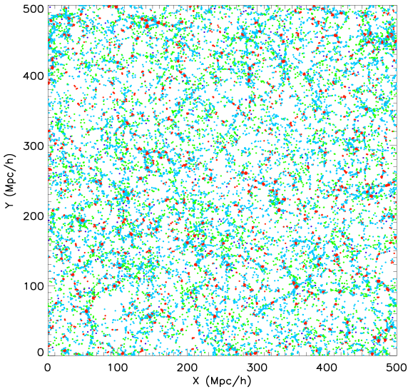
Figure 1.— Projected distribution of halos within a $2\>h^{-1}{\rm{Mpc}}$ thick slice. For clarity, only randomly selected 20% halos with masses larger than $10^{10}\>h^{-1}\rm M_{\odot}$ are shown and color coded in red, cyan, green and blue colors accordingly to their cosmic web environments: clusters, filaments, sheets and voids, respectively.

2. Data and method

2.1. Halos in the ELUCID simulation

In this study we use dark matter halos extracted from the ELUCID (Exploring the Local Universe with re-Constructed Initial Density field) simulation. This simulation which evolves the distribution of $3072^{3}$ dark matter particles in a periodic box of $500\>h^{-1}{\rm{Mpc}}$ on a side was carried out in the Center for High Performance Computing, Shanghai Jiao Tong University. The simulation was run with L-GADGET, a memory optimized version of GADGET2 (Springel, 2005). The cosmological parameters adopted by this simulation are consistent with WMAP5 results with a mass per particle of $3.0875\times 10^{8}\>h^{-1}\rm M_{\odot}$.

Even though this is not relevant to this particular study, the ELUCID simulation is a reconstruction of the mass density field extracted from the galaxy (e.g. Blanton et al., 2005) and group (e.g. Yang et al., 2007) distribution in the north galactic pole region of the SDSS Data Release 7 (Abazajian et al., 2009). This density field has been used to constrain the initial conditions using a Hamiltonian Markov Chain Monte Carlo method with particle mesh dynamics (ELUCID I: Wang et al., 2014). The genesis of the ELUCID simulation in particular and its basic properties such as the output power spectrum and halo mass functions are described in detail in Wang et al. (2016, ELUCID III).

Dark matter halos have been identified in the ELUCID simulation with the friends-of-friends algorithm. We have used a linking length of $0.2$ times the mean particle separation. Only halos containing at least $20$ particles are used for our study. The dark matter halo mass function of this simulation at redshift $z=0$ is in very good agreement with the theoretical predictions of Sheth, Mo, & Tormen (2001) and Tinker et al. (2008).

2.2. Separating halos into different cosmic web types

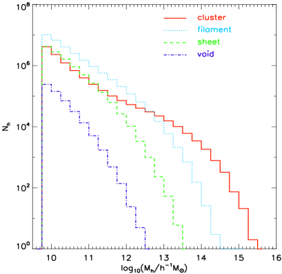
Figure 2.— Mass distribution of halos. Red, cyan, green and blue lines indicate the mass distributions for halos in cluster, filament, sheet and void environments, respectively.

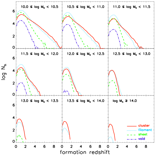
Figure 3.— Formation redshift of halos within different cosmic web environments. Each panel correspond to a specific halo mass bin. Red, cyan, green and blue lines indicate the formation redshift distributions for halos in cluster, filament, sheet and void environments, respectively.

In order to probe the clustering properties of halos within different cosmic web environments, we first classify the dark matter halos’ environment using the method by Zhang et al. (2009). This method is based on the Hessian matrix of the smoothed density field. This matrix is defined as

$$H_{i,j}=\frac{\partial^{2}\rho_{s}}{\partial x_{i}\partial x_{j}},$$ (1)

where the Hessian matrix indices $i$ and $j$ and the corresponding coordinates $x_{i}$ and $x_{j}$ can take values from the cartesian coordinates along the box axis $x$, $y$ and $z$. The smoothed density field $\rho_{s}$ is calculated using a Gaussian filter with a smoothing scale $R_{s}=2.1\>h^{-1}{\rm{Mpc}}$ (Hahn et al., 2007a; Zhang et al., 2009). The 3 eigenvalues $\lambda_{[1,2,3]}$ of the Hessian matrix $H_{i,j}$ are then calculated at the position of each halo. We adopt the convention where $\lambda_{1}\leq\lambda_{2}\leq\lambda_{3}$. The number of negative eigenvalues of $H_{i,j}$ can be used to classify the environment in which the halo resides as follows (see Zhang et al., 2009):

cluster

a point where all three eigenvalues are negative,
$\lambda_{1}\leq\lambda_{2}\leq\lambda_{3}<0$;

filament

a point with 2 negative eigenvalues,
$\lambda_{1}\leq\lambda_{2}<0<\lambda_{3}$;

sheet

a point with only 1 negative eigenvalue,
$\lambda_{1}<0<\lambda_{2}\leq\lambda_{3}$;

void

a point with no negative eigenvalues,
$0<\lambda_{1}\leq\lambda_{2}\leq\lambda_{3}$.

Of the $48,129,323$ halos at redshift $z=0$ in the ELUCID simulation, $9,529,790$ $(19.8\%)$ are located in clusters, $27,439,946$ $(57.0\%)$ are located in filaments, $10,649,415$ $(22.1\%)$ are located in sheets and $510,172$ $(1.1\%)$ are located in voids. Fig. 1 shows the projected distribution of dark matter halos in the ELUCID simulation in a $500\>h^{-1}{\rm{Mpc}}\times 500\>h^{-1}{\rm{Mpc}}$ slice of thickness $2\>h^{-1}{\rm{Mpc}}$. Halos in clusters, filaments, sheets, and voids are indicated with red, cyan, green and blue colors, respectively.

We show in Fig. 2 the mass distributions of halos in different cosmic web environments. Halos are the least numerous in the voids and are more numerous in the filaments than in the sheets. In the clusters, the number of halos obeys a different trend. At low mass ($M_{\rm h}<10^{11.5}\>h^{-1}\rm M_{\odot}$) end, this number lies between those obtained for voids and sheets and at intermediate mass range ($10^{11.5}<M_{\rm h}<10^{12.5}\>h^{-1}\rm M_{\odot}$) between those of sheet and filament numbers. As higher and higher masses are explored, halos in clusters increasingly dominate the whole population.

The formation of dark matter halos is a complex physical process which can be characterized through a timescale: the halo formation time. Among the various existing definition found in the literature, we use the most common one which corresponds to the time at which the halo’s main branch assembled half of its present (redshift $z=0$) mass $M_{\rm h}$. Fig. 3 shows the distribution of halos as a function of their formation redshift. The different cosmic web environments are distinguished and denoted by different colors. Each panel corresponds to a different halo mass range as indicated. The age distribution of halos are quite similar in the filaments, sheets and voids. The halos in clusters however, show broader age distributions, especially for low mass ones. Nevertheless, the peak formation redshifts of halos in all four cosmic web environments are similar, which gradually change from $z\sim 1$ in low mass halos to $z\sim 0.5$ in massive halos. In addition, we find that low mass halos ($M_{\rm h}<10^{11.0}\>h^{-1}\rm M_{\odot}$) in clusters (red) are slightly older than halos of the same mass that reside in voids (blue).

2.3. Cross correlation and auto correlation functions

With all the halos being classified as part of different cosmic web environments, we proceed to probe their clustering properties. The first quantity we measure is the cross correlation function (CCF) between halos and dark matter particles,

$$\xi_{\rm CCF}(r)=\frac{P_{\rm HD}(r)}{P_{\rm HR}(r)}-1\,,$$ (2)

where $P_{\rm HD}(r)$ and $P_{\rm HR}(r)$ are the number of halo-dark matter and halo-random pairs, respectively. For our investigations, the number of random points has been set to be the same as the number of dark matter particles within the simulation box. Those points follow a uniform distribution within the simulation volume.

In order to ensure self-consistency of the CCFs, we also measure the auto correlation function (ACF) of dark matter halos,

$$\xi_{\rm ACF}(r)=\frac{N_{\rm R}^{2}P_{\rm HH}(r)}{N_{\rm H}^{2}P_{\rm RR}(r)}-1\,,$$ (3)

where $P_{\rm HH}(r)$ and $P_{\rm RR}(r)$ are the number of halo-halo and random-random pairs, $N_{\rm H}$ and $N_{\rm R}$ are the number of halos and random points, respectively.

3. The clustering properties of halos in different cosmic web environments

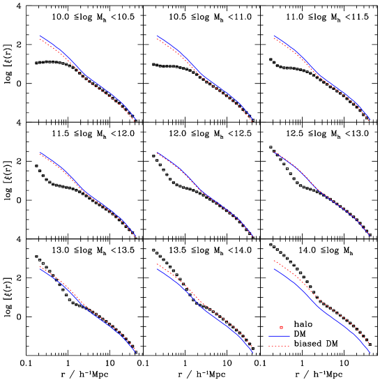
Figure 4.— Cross correlation functions between halos and dark matter particles. The different panels correspond to the same mass ranges as in Fig. 3. Results are shown with open squares and error bars. For reference, the solid lines indicate the dark matter auto correlation in the ELUCID simulation and the dotted lines the same auto correlation multiplied by the bias factor of the halos in consideration.

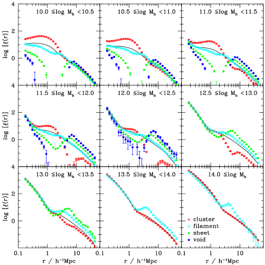
Figure 5.— Same as Fig. 4, but for halos in different cosmic web environments. In each panel, the open squares, open circles, stars and dots are results for halos in different cosmic web environments: clusters, filaments, sheets and voids, respectively. For comparison, results for the overall population are represented using a solid line.

3.1. Halo cross correlations

We first measure the CCFs between halos and dark matter particles in the ELUCID simulation. We use the subsamples introduced in Fig 3, namely 9 mass ranges ($\Delta\log M_{h}=0.5$): $10.0\leq\log M_{h}<10.5$, $10.5\leq\log M_{h}<11.0$, … $14.0\leq\log M_{h}$. The open squares shown in Fig. 4 are the CCFs measured from halos within these mass bins. The error bars are obtained from 200 bootstrap re-samplings of the dark matter halos. There are two features in these CCFs:

1. more massive halos have overall stronger CCFs;

2. the 1-halo and 2-halo terms in the CCFs can be clearly separated by a change in the slope.

For comparison, we also measured the auto correlation function (ACF) of dark matter particles in the ELUCID simulation. It is shown in each panel of Fig. 4 as a solid line. Quite interestingly, the CCF of halos with mass $\lesssim 10^{13.5}\>h^{-1}\rm M_{\odot}$ is much smaller than the ACF at the 1-halo and 2-halo transition scales. This is caused by the lack of 1-halo pairs in the CCF. On larger scales, $r\gtrsim 3\>h^{-1}{\rm{Mpc}}$, the shape of CCF is quite consistent with the ACF. Since massive halos are more strongly clustered (biased) than low mass ones, to take this bias into account in the ACF we use the theoretical predictions obtained by Tinker et al. (2010). The dotted line in each panel is the ACF of dark matter particles multiplied by the median bias factor for the halos in consideration. In general, we find that the biased ACFs on large scales are in nice agreement with the CCFs.

Once we measured the CCFs of halos in different mass bins, we proceed to measure the CCFs of subsamples of halos in different cosmic web environments. We show in Fig 5 the CCFs measured separately from the four halo subsamples corresponding to their large scale environments, namely: clusters (red open squares), filaments (cyan open circles), sheets (green filled pentagons) and voids (blue filled circles). The CCFs of these subsamples show quite different behaviors compared to the overall halo sample. This is a clear indication that a significant cosmic web environment dependence exists, both on intermediate and large scales. More precisely, this figure reveals the following features:

1. On very small scales, where the CCFs are dominated by the 1-halo term, the CCFs of halos in different cosmic web environments follows the expected asymptotic trends. This behavior may not appear clearly for halos $\lesssim 10^{11.0}\>h^{-1}\rm M_{\odot}$ as the scale is limited to values $\gtrsim 0.15\>h^{-1}{\rm{Mpc}}$. Still it is quite distinct in more massive halos.

2. At intermediate scales between the 1-halo term region and $\sim 3\>h^{-1}{\rm{Mpc}}$, some interesting variations are revealed especially for relatively low mass $\lesssim 10^{12.5}\>h^{-1}\rm M_{\odot}$ halos. Halos in cluster, filament, sheet and void environments sequentially show suppressed CCFs. This feature is again quite expected, as the cosmic web environments themselves are defined according to the density field on such scales.

3. On large scales at $\gtrsim 8\>h^{-1}{\rm{Mpc}}$, however, an interesting and unexpected feature is found in the CCFs. The halos in cluster, filament, sheet and void environments sequentially show enhanced CCFs. At any fixed mass, halos in the void region have the highest bias.

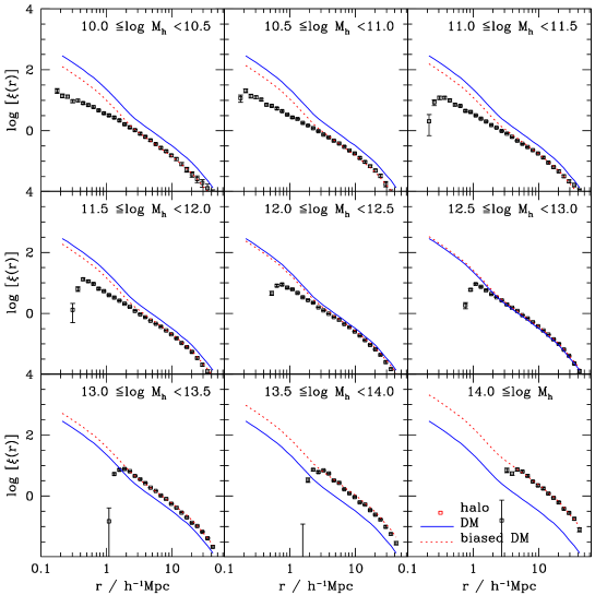
Figure 6.— Same as Fig, 4, but for the halo auto correlation functions.

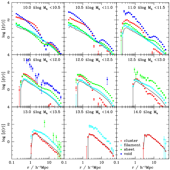
Figure 7.— Same as Fig, 5, but for the halo auto correlation functions.

Table 1The biases of halos in different cosmic web environments.

(1)	(2)	(3)	(4)	(5)	(6)	(7)
ID	$\log M_{h}$	All	Cluster	Filament	Sheet	Void
1	10.20	0.799 $\pm$ 0.063	0.897 $\pm$ 0.054	0.753 $\pm$ 0.127	0.829 $\pm$ 0.081	1.171 $\pm$ 0.041
2	10.70	0.822 $\pm$ 0.084	0.633 $\pm$ 0.049	0.691 $\pm$ 0.060	0.867 $\pm$ 0.046	1.456 $\pm$ 0.097
3	11.20	0.672 $\pm$ 0.049	0.438 $\pm$ 0.054	0.802 $\pm$ 0.123	1.194 $\pm$ 0.082	2.165 $\pm$ 0.057
4	11.70	0.785 $\pm$ 0.070	0.272 $\pm$ 0.090	0.836 $\pm$ 0.090	1.624 $\pm$ 0.058	3.116 $\pm$ 0.274
5	12.20	0.845 $\pm$ 0.036	0.159 $\pm$ 0.092	1.077 $\pm$ 0.098	2.387 $\pm$ 0.056	4.451 $\pm$ 0.801
6	12.70	1.112 $\pm$ 0.048	0.369 $\pm$ 0.043	1.663 $\pm$ 0.115	3.487 $\pm$ 0.171	–
7	13.20	1.248 $\pm$ 0.075	0.896 $\pm$ 0.066	2.459 $\pm$ 0.156	4.692 $\pm$ 0.703	–
8	13.70	1.695 $\pm$ 0.056	1.502 $\pm$ 0.051	3.645 $\pm$ 0.121	–	–
9	14.20	2.711 $\pm$ 0.098	2.716 $\pm$ 0.106	–	–	–
10	10.20	0.697 $\pm$ 0.050	0.902 $\pm$ 0.020	0.701 $\pm$ 0.032	0.751 $\pm$ 0.025	1.080 $\pm$ 0.054
11	10.70	0.703 $\pm$ 0.055	0.646 $\pm$ 0.039	0.727 $\pm$ 0.040	0.935 $\pm$ 0.031	1.515 $\pm$ 0.022
12	11.20	0.770 $\pm$ 0.069	0.432 $\pm$ 0.018	0.726 $\pm$ 0.043	1.144 $\pm$ 0.034	2.057 $\pm$ 0.209
13	11.70	0.765 $\pm$ 0.016	0.291 $\pm$ 0.052	0.875 $\pm$ 0.022	1.595 $\pm$ 0.084	3.514 $\pm$ 0.387
14	12.20	0.831 $\pm$ 0.045	0.324 $\pm$ 0.044	1.104 $\pm$ 0.038	2.316 $\pm$ 0.200	–
15	12.70	1.035 $\pm$ 0.039	0.522 $\pm$ 0.049	1.642 $\pm$ 0.076	3.416 $\pm$ 0.367	–
16	13.20	1.286 $\pm$ 0.052	0.953 $\pm$ 0.066	2.448 $\pm$ 0.080	–	–
17	13.70	1.621 $\pm$ 0.090	1.465 $\pm$ 0.087	3.647 $\pm$ 0.764	–	–
18	14.20	2.618 $\pm$ 0.126	2.633 $\pm$ 0.105	–	–	–

Note. — Column (1): ID. Results listed in rows 1-9 are obtained from CCFs, 10-18 are obtained from ACFs. Column (2): logarithm of the halo mass. Column (3): average biases of halos of overall population. Columns (4)-(7): average biases of halos in the cluster, filament, sheet and void environments, respectively.

3.2. Halo auto correlations

The clustering strengths of large scale CCFs in different cosmic web environments obviously contradict our naive expectation that halos in voids should be less clustered. To test the robustness of these findings, we proceed to calculate the halo ACFs.

Similar to the CCFs, we first measure the ACFs of halos that are separated into nine samples in different mass ranges: $10.0\leq\log M_{h}<10.5$, $10.5\leq\log M_{h}<11.0$, … $14.0\leq\log M_{h}$. The open squares shown in Fig. 6 are the ACFs we measured from these halos. The error bars are once again obtained from 200 bootstrap re-samplings of the dark matter halos. We also show, for comparison, the ACF of dark matter particles as solid line, and the biased ACF as dotted one. The later is obtained by multiplying the unbiased ACF by the square of the median bias factor of those halos in consideration. Similarly to the CCFs, we find that the ACFs of halos are quite consistent with the biased ACFs of dark matter particles on large scales. The small scale ACFs cut off is especially apparent for massive halos. These are caused by the halo-halo exclusion effect as modeled in Wang et al. (2004). Overall, the ACFs in different mass bins behave as expected.

Next, we proceed to measure the ACFs for halos in different cosmic web environments. Shown in each panel of Fig. 7 are the ACFs for halos in different cosmic web environments: clusters, filaments, sheets and voids. These ACFs show quite different behaviors compared to the overall sample. This further indicates that a significant cosmic web environment dependence exists. On small to intermediate scales, the clustering properties of ACFs are different from CCFs, especially for the halos in the voids where they show overall stronger clusterings. Nevertheless, the clustering behaviors on these scales are not the main focus of this probe. The most exciting feature is that, on scales $\gtrsim 15\>h^{-1}{\rm{Mpc}}$, the halos show the same cosmic web environment dependence as the CCFs, where strongest clustering strength is revealed in the ACFs of void halos.

The cosmic web dependence of the clustering strengths found here is opposite to that obtained by Fisher & Faltenbacher (2016), who claimed that halo bias monotonically increases with cosmic web environments from voids to clusters. Although it is unclear to us what is the main cause of such a discrepancy, one possibility is that they used the velocity shear tensor to classify halos into different cosmic web types. Nevertheless, in a very recent study using a Fourier analysis method, Paranjape et al. (2017) found the same trends of halo biases as ours: the halos in filaments have significantly larger biases than those in clusters. Coming back to the strongest clustering strength of void halos, one intuitive explanation is that the clustering of void halos might be composed of the void-void correlation weighted by the void occupation numbers.

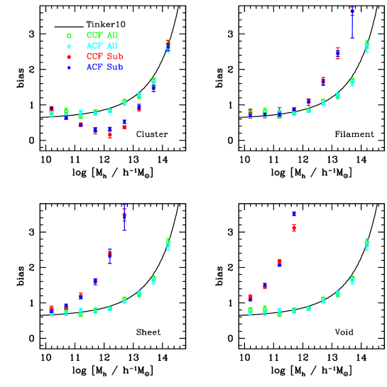
Figure 8.— Halo biases as a function of halo mass. Each panel refers to a different cosmic web environment. Halo biases calculated using the CCFs and ACFs of the overall population are shown with open circles and squares, respectively. The ones obtained from CCFs and ACFs of halo subsamples are displayed as solid circles and squares, respectively. For comparison, the model prediction of Tinker et al. (2010) is indicated by the solid line.

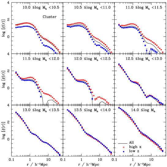
Figure 9.— Cross correlation functions between halos in the clusters and the dark matter particles. In each panel, the open squares and solid dots focuses on the 20% oldest and 20% youngest halos, respectively. For comparison, we also show using a solid line the results for overall population.

3.3. Cosmic web dependent halo bias

In order to quantify the overall clustering strengths of halos within different cosmic web environments, we measure the average biases of halos. These average biases are measured using the ratios between the halo CCFs and the dark matter particles’ ACFs within radii $15<r<45\>h^{-1}{\rm{Mpc}}$ as shown in Fig. 4. In all panels of Fig. 8 and displayed with open circles are the average biases thus measured for overall population as a function of halo mass. The error bars indicate the variances of the CCF ratios (biases) at different radii. Once again we use the halo ACFs to confirm those measurements, and display as open squares the average square root ratios between the ACFs of halos and dark matter particles within radii $15<r<45\>h^{-1}{\rm{Mpc}}$. This second measurements of the average biases obtained agree very well with those obtained from the CCFs. For completeness, we have added to the figure a solid line representing theoretical model prediction by Tinker et al. (2010). The average biases of halos measured from the ELUCID simulation show an overall very nice agreement with the model.

In addition to the generic features relevant to the overall population we have just mentioned, each panel is used to distinguish a specific cosmic web environment for which the halo bias measurements are repeated. Environmental bias measurement made using the CCF are shown as red filled circles. While the ones made using the ACF are shown as filled squares. The average biases of halos in the clusters (upper-left panel of Fig. 8) agree with the overall population on both massive and low mass end, but are significantly suppressed for intermediate mass halos. The average biases of halos with mass $\sim 10^{12.0}\>h^{-1}\rm M_{\odot}$ is almost by a factor of 3 lower than the overall population. Compared to those in clusters, halos in filaments (upper-right panel) show significantly enhanced biases, especially at the massive end with mass $\gtrsim 10^{12.5}\>h^{-1}\rm M_{\odot}$. Shown in the lower-left and lower-right panels of Fig. 8 are the average biases of halos in the sheets and the voids, respectively. Again we see a clear trend that halos in the sheets and voids are ever increasingly enhanced. Overall, the clustering strength of halos increases significantly from the clusters to the voids, with stronger impact in more massive halos. For instance, Milky Way sized halos (mass $\sim 10^{12.0}\>h^{-1}\rm M_{\odot}$) in the voids have bias $\gtrsim 3$, which is even larger than the overall clustering strength of cluster sized halos.

Finally, for reference, the related biases of halos in different cosmic web environments are listed in Table 1. Such a strong cosmic web dependent halo bias may play important roles in cosmological and galaxy formation probes. For instance, Hamaus et al. (2014) proposed a method of using galaxy-void cross correlation to constrain cosmologies, the very different clustering behaviors of void halos found here must be properly taken into account in such kind of studies. On the other hand, as pointed out in ELUCID III, the fractions of red galaxies as functions of the $r$-band absolute magnitude depend very strongly on the cosmic web environments. It would be very interesting to see if galaxies in different cosmic web environments have different galaxy-halo connections. For this purpose, the very different halo biases in different cosmic web environments have to be taken into account in establishing the galaxy-halo connections using the HOD or CLF models.

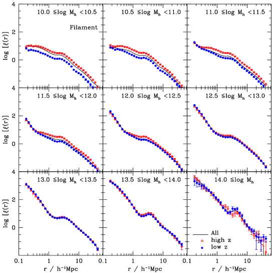
Figure 10.— Similar to Fig. 9, but for halos in the filaments.

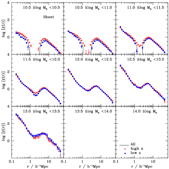
Figure 11.— Similar to Fig. 9, but for halos in the sheets.

Figure 12.— Similar to Fig. 9, but for halos in the voids.

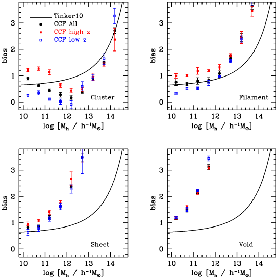
Figure 13.— Halo biases as a function of halo mass. Each panel represent a different cosmic web environment. Halo biases are computed using the CCF from all halos (filled black circle), the 20% oldest (filled red squares) and the 20% youngest (open blue squares) halos. For comparison, we also show the model prediction of Tinker et al. (2010) using a solid line.

Figure 14.— Similar to Fig. 13, but here for halos in the controlled samples. The results shown in the lower-right panel for void halos are the same as those in Fig. 13. Halo biases computed in other panels for the 20% oldest (filled red squares) and the 20% youngest (open blue squares) are obtained from the controlled samples.

4. Assembly bias of halos in different cosmic web environments

In recent years, great effort has been made to quantify the assembly bias of halos, among which the most notable one is the age dependence. Having quantified the cosmic web environment dependence of halo biases, we come to the second purpose of this work: to investigate whether or not the age dependent biases of halos can be explained using the cosmic web environment dependent halo biases. More precisely we try to confirm the presence or absent of prominent age dependent biases for halos in different cosmic web environments. To this end, we separate halos in the two tails of the formation redshift distribution, building 2 sets of halo sub-subsamples representing the 20% oldest and 20% youngest ones and measure separately their clustering properties.

We first measure the CCFs of halos in the clusters. The open squares and solid dots in Fig. 9 indicate the resulting CCFs for the oldest (high z) and youngest (low z) halos. For halos with mass $\lesssim 10^{12.5}\>h^{-1}\rm M_{\odot}$, the clustering strengths of the two sub-subsamples are quite different, the oldest sub-subsample having much stronger clustering strength than the youngest sub-subsample. However, for more massive halos, the two CCFs are quite consistent with one another indicating a lack of assembly bias. As the assembly bias features found in Gao et al. (2005) are prominent within mass range $\lesssim 10^{13.5}\>h^{-1}\rm M_{\odot}$, or $\lesssim 10^{13.0}\sim 10^{13.5}\>h^{-1}\rm M_{\odot}$ for different definitions of formation time (see, e.g. Li et al., 2008), the assembly bias feature found here is at least limited to a smaller mass range.

Next, we focus on the filaments, where the results are shown in Fig. 10 following the same legend as Fig. 9. Compared to halos in the clusters, the assembly bias features differ in two aspects: (1) the overall strength decreases and (2) the reduction is more significant in more massive halos.

Finally in Figs. 11 and 12, we show the halo CCFs respectively in the sheets and the voids. Compared to the clusters and the filaments, assembly bias features are further reduced in the sheets, especially in terms of amplitude. In the void environment, halo assembly bias features are no longer apparent, with the oldest and youngest halos overlapping with the overall void halo population.

In order to quantify the assembly biases for halos in different cosmic web environments, we use once again the ratios of the halo CCFs shown in Figs. 9 - 12 and the dark matter ACFs within radii $15<r<45\>h^{-1}{\rm{Mpc}}$. The average bias measurements are displayed as a function of mass in Fig. 13, with each panel corresponding to a specific environment. In each panel, the biases for overall population, oldest 20% and youngest 20% halos are shown using solid dots, solid squares and open squares, respectively. The error bars again are obtained using the variances of the CCF ratios (biases) at different radii. For the cluster environment in the upper-left panel, the assembly biases is clearly apparent with the oldest and youngest halos results being located respectively above and below the overall cluster population. The assembly bias of halos in clusters is found here to be of similar amplitude to the one measured by Gao et al. (2005). However it appears in our case in less massive halos with mass $\lesssim 10^{12.5}\>h^{-1}\rm M_{\odot}$. As we explore the filament environment (upper-right panel) we notice a reduction in the amplitude of the assembly biases. The reduction is even more pronounced in the sheets (lower-left panel) and the assembly bias entirely absents in the voids (lower right panel).

Note however, as the halos in different environments have different age distributions (see Fig. 3), we carry out an additional test to check if the reduction of assembly bias, especially that in voids, is really due to the fixed environment. Here we take the halos in the voids as the reference sample and select a set of controlled halo samples from other environments that match the same mass and formation time distributions. Following the same procedures we carried out for the reference sample in voids, we measure the biases of the oldest 20% and youngest 20% halos in the controlled samples in clusters, filaments, and sheets, respectively. Thus obtained results are shown in Fig. 14. Here only halos with mass $\leq 10^{12.5}\>h^{-1}\rm M_{\odot}$ are used for our investigation. Compare to the original halos shown in Fig. 13, the ones in the controlled samples show very similar, although somewhat less prominent, assembly bias features. These features indicate that the reduction of assembly bias from clusters, filaments to sheets and voids is real.

Although the results are not displayed in the paper, the measurements using the ACF alternatives (as in Fig. 8) were performed and found to give very similar results.

5. Summary

In this paper, we have probed the clustering properties of halos in different cosmic web environments using the ELUCID simulation. Halos were separated into four cosmic web environments defined through the Hessian matrix of the smoothed density field. Out of a total of $48,129,323$ halos in the ELUCID simulation, $19.8\%$ are located in cluster, $57.0\%$ in filaments, $22.1\%$ in sheets and $1.1\%$ in voids. In order to probe the related mass dependence of the clustering properties, we also separated the halos into nine halo mass bins, $10.0\leq\log M_{h}<10.5$, …, $13.5\leq\log M_{h}<14.0$ and $14.0\leq\log M_{h}$. Furthermore, so as to confirm existing age dependent assembly biases in different cosmic web environments, additional subsamples were made based on the formation redshift focussing on the 20% oldest and 20% youngest halos.

We have measured the cross correlation functions between halos and dark matter particles, as well as the related auto correlation functions of halos in these subsamples. The ratios between the halo CCFs (or ACFs) and the dark matter ACFs within radii $15<r<45\>h^{-1}{\rm{Mpc}}$ are used to estimate the average biases of halos. We find significantly different biases for halos of same masses but in different cosmic web environments. We summarize our main results as follows;

• The average biases of halos in clusters agree with the overall population on both high and low mass ends, but are significantly suppressed in intermediate mass scales. The average biases of halos with mass $\sim 10^{12.0}\>h^{-1}\rm M_{\odot}$ are almost by a factor of 3 lower than the overall population.

• The halos in filaments show significantly enhanced biases, especially at the massive end with mass $\gtrsim 10^{12.5}\>h^{-1}\rm M_{\odot}$ .

• Halos in sheets show stronger enhanced biases as a function of halo mass.

• Halos in voids show the strongest bias enhancements. The Milky Way sized halos with mass $\sim 10^{12.0}\>h^{-1}\rm M_{\odot}$ in void region have bias $\gtrsim 3$, which is even larger than the overall clustering strength of cluster sized halos.

• The strength of the assembly biases (age dependences) decreases from cluster, filament and sheet environments to finally disappears in void environment.

• In addition, the age dependent assembly biases of halos in different cosmic web environments exist in a smaller mass range $\lesssim 10^{12.5}\>h^{-1}\rm M_{\odot}$, compared to the overall population at $\lesssim 10^{13.0}\sim 10^{13.5}\>h^{-1}\rm M_{\odot}$.

As we have found very prominent – as strong as the mass dependence – cosmic web environment dependence of halo biases, a similar study focussed on galaxy clustering in different cosmic web environments would be relevant. It would indeed be interesting to obtain the galaxy-halo connections in different cosmic web environments, which can be used to better constrain galaxy formation models and better understand the void-galaxy clustering properties for cosmological studies, etc.

References

- Abazajian et al. (2009) Abazajian, K. N., Adelman-McCarthy, J. K., Agüeros, M. A., et al. 2009, ApJS, 182, 543
- Aragón-Calvo et al. (2007a) Aragón-Calvo, M. A., van de Weygaert, R., Jones, B. J. T., & van der Hulst, J. M. 2007, ApJ, 655, L5
- Aragón-Calvo et al. (2007b) Aragón-Calvo, M. A., Jones, B. J. T., van de Weygaert, R., & van der Hulst, J. M. 2007, A&A, 474, 315
- Bahcall et al. (2003) Bahcall, N. A., Dong, F., Hao, L., et al. 2003, ApJ, 599, 814
- Bardeen et al. (1986) Bardeen, J. M., Bond, J. R., Kaiser, N., & Szalay, A. S. 1986, ApJ, 304, 15
- Berlind & Weinberg (2002) Berlind, A. A., & Weinberg, D. H. 2002, ApJ, 575, 587
- Blanton et al. (2005) Blanton, M. R., Schlegel, D. J., Strauss, M. A., et al. 2005, AJ, 129, 2562
- Blanton & Berlind (2007) Blanton, M. R., & Berlind, A. A. 2007, ApJ, 664, 791
- Borzyszkowski et al. (2017) Borzyszkowski, M., Porciani, C., Romano-Díaz, E., & Garaldi, E. 2017, MNRAS, 469, 594
- Croton et al. (2007) Croton, D. J., Gao, L., & White, S. D. M. 2007, MNRAS, 374, 1303
- Colless et al. (2001) Colless, M., Dalton, G., Maddox, S., et al. 2001, MNRAS, 328, 1039
- Cooray & Sheth (2002) Cooray, A., & Sheth, R. 2002, Phys. Rep., 372, 1
- Dai (2015) Dai, D.-C. 2015, MNRAS, 454, 3590
- Dalal et al. (2008) Dalal, N., White, M., Bond, J. R., & Shirokov, A. 2008, ApJ, 687, 12-21
- Deason et al. (2013) Deason, A. J., Conroy, C., Wetzel, A. R., & Tinker, J. L. 2013, ApJ, 777, 154
- Driver et al. (2011) Driver, S. P., Hill, D. T., Kelvin, L. S., et al. 2011, MNRAS, 413, 971
- Dunkley et al. (2009) Dunkley J., et al., 2009, ApJS, 180, 306
- Eardley et al. (2015) Eardley, E., Peacock, J. A., McNaught-Roberts, T., et al. 2015, MNRAS, 448, 3665
- Fisher & Faltenbacher (2016) Fisher, J. D., & Faltenbacher, A. 2016, arXiv:1603.06955
- Gao et al. (2005) Gao, L., Springel, V., & White, S. D. M. 2005, MNRAS, 363, L66
- Gao & White (2007) Gao, L., & White, S. D. M. 2007, MNRAS, 377, L5
- Hamaus et al. (2014) Hamaus, N., Wandelt, B. D., Sutter, P. M., Lavaux, G., & Warren, M. S. 2014, Physical Review Letters, 112, 041304
- Hamaus et al. (2016) Hamaus, N., Pisani, A., Sutter, P. M., et al. 2016, Physical Review Letters, 117, 091302
- Hahn et al. (2007a) Hahn, O., Porciani, C., Carollo, C. M., & Dekel, A. 2007a, MNRAS, 375, 489
- Hahn et al. (2007b) Hahn, O., Carollo, C. M., Porciani, C., & Dekel, A. 2007b, MNRAS, 381, 41
- Hearin et al. (2015) Hearin, A. P., Watson, D. F., & van den Bosch, F. C. 2015, MNRAS, 452, 1958
- Hearin et al. (2016) Hearin, A. P., Zentner, A. R., van den Bosch, F. C., Campbell, D., & Tollerud, E. 2016, MNRAS, 460, 2552
- Jing (1998) Jing, Y. P. 1998, ApJ, 503, L9
- Jing et al. (1998) Jing, Y. P., Mo, H. J., & Börner, G. 1998, ApJ, 494, 1
- Jung et al. (2014) Jung, I., Lee, J., & Yi, S. K. 2014, ApJ, 794, 74
- Lacerna et al. (2014) Lacerna, I., Padilla, N., & Stasyszyn, F. 2014, MNRAS, 443, 3107
- Lee et al. (2017) Lee, C. T., Primack, J. R., Behroozi, P., et al. 2017, MNRAS, 466, 3834
- Li et al. (2008) Li, Y., Mo, H. J., & Gao, L. 2008, MNRAS, 389, 1419
- Lin et al. (2016) Lin, Y.-T., Mandelbaum, R., Huang, Y.-H., et al. 2016, ApJ, 819, 119
- Mao et al. (2017) Mao, Y.-Y., Zentner, A. R., & Wechsler, R. H. 2017, arXiv:1705.03888
- Miyatake et al. (2016) Miyatake, H., More, S., Takada, M., et al. 2016, Physical Review Letters, 116, 041301
- Mo & White (1996) Mo, H. J., & White, S. D. M. 1996, MNRAS, 282, 347
- More et al. (2016) More, S., Miyatake, H., Takada, M., et al. 2016, ApJ, 825, 39
- Paranjape et al. (2017) Paranjape, A., Hahn, O., & Sheth, R. K. 2017, arXiv:1706.09906
- Pillepich et al. (2010) Pillepich, A., Porciani, C., & Hahn, O. 2010, MNRAS, 402, 191
- Press & Schechter (1974) Press, W. H., & Schechter, P. 1974, ApJ, 187, 425
- Pujol et al. (2017) Pujol, A., Hoffmann, K., Jiménez, N., & Gaztañaga, E. 2017, A&A, 598, A103
- Reed et al. (2007) Reed, D. S., Governato, F., Quinn, T., Stadel, J., & Lake, G. 2007, MNRAS, 378, 777
- Seljak & Warren (2004) Seljak, U. & Warren, M. S. 2004, MNRAS, 355, 129
- Sheth & Tormen (1999) Sheth, R. K., & Tormen, G. 1999, MNRAS, 308, 119
- Sheth, Mo, & Tormen (2001) Sheth R. K., Mo H. J., Tormen G., 2001, MNRAS, 323, 1
- Sheth & Tormen (2004) Sheth, R. K., & Tormen, G. 2004, MNRAS, 350, 1385
- Springel (2005) Springel V., 2005, MNRAS, 364, 1105
- Swanson et al. (2008) Swanson, M. E. C., Tegmark, M., Blanton, M., & Zehavi, I. 2008, MNRAS, 385, 1635
- Tinker et al. (2005) Tinker, J. L., Weinberg, D. H., Zheng, Z., & Zehavi, I. 2005, ApJ, 631, 41
- Tinker et al. (2008) Tinker, J., Kravtsov, A. V., Klypin, A., et al. 2008, ApJ, 688, 709-728
- Tinker et al. (2010) Tinker, J. L., Robertson, B. E., Kravtsov, A. V., et al. 2010, ApJ, 724, 878
- Tojeiro et al. (2016) Tojeiro, R., Eardley, E., Peacock, J. A., et al. 2016, arXiv:1612.08595
- Tonnesen & Cen (2015) Tonnesen, S., & Cen, R. 2015, ApJ, 812, 104
- van den Bosch et al. (2003) van den Bosch, F. C., Yang, X., & Mo, H. J. 2003, MNRAS, 340, 771
- Wang et al. (2004) Wang Y., Yang X., Mo H.J., van den Bosch F.C., Chu Y., 2004, MNRAS, 353, 287
- Wang et al. (2009) Wang, H., Mo, H. J., Jing, Y. P., et al. 2009, MNRAS, 394, 398
- Wang et al. (2012) Wang, H., Mo, H. J., Yang, X., & van den Bosch, F. C. 2012, MNRAS, 420, 1809
- Wang et al. (2014) Wang, H., Mo, H. J., Yang, X., Jing, Y. P., & Lin, W. P. 2014, ApJ, 794, 94, ELUCID I
- Wang et al. (2016) Wang, H., Mo, H. J., Yang, X., et al. 2016, ApJ, 831, 164, ELUCID III
- Wang et al. (2011) Wang, H., Mo, H. J., Jing, Y. P., Yang, X., & Wang, Y. 2011, MNRAS, 413, 1973
- Wang et al. (2013) Wang, L., Weinmann, S. M., De Lucia, G., & Yang, X. 2013, MNRAS, 433, 515
- Wang et al. (2008) Wang, Y., Yang, X., Mo, H. J., et al. 2008, ApJ, 687, 919-935
- Wechsler et al. (2006) Wechsler, R. H., Zentner, A. R., Bullock, J. S., Kravtsov, A. V., & Allgood, B. 2006, ApJ, 652, 71
- Yang et al. (2003) Yang, X., Mo, H. J., & van den Bosch, F. C. 2003, MNRAS, 339, 1057
- Yang et al. (2005) Yang, X., Mo, H. J., van den Bosch, F. C., & Jing, Y. P. 2005, MNRAS, 357, 608
- Yang et al. (2006) Yang, X., Mo, H. J., & van den Bosch, F. C. 2006, ApJ, 638, L55
- Yang et al. (2007) Yang X., Mo H. J., van den Bosch F. C., Pasquali A., Li C., Barden M., 2007, ApJ, 671, 153
- Yang et al. (2012) Yang, X., Mo, H. J., van den Bosch, F. C., Zhang, Y., & Han, J. 2012, ApJ, 752, 41
- Zentner et al. (2014) Zentner, A. R., Hearin, A. P., & van den Bosch, F. C. 2014, MNRAS, 443, 3044
- Zhang et al. (2009) Zhang, Y., Yang, X., Faltenbacher, A., et al. 2009, ApJ, 706, 747
- Zu et al. (2008) Zu, Y., Zheng, Z., Zhu, G., & Jing, Y. P. 2008, ApJ, 686, 41-52
- Zu et al. (2017) Zu, Y., Mandelbaum, R., Simet, M., Rozo, E., & Rykoff, E. S. 2017, MNRAS, 470, 551