Dissipative Quantum Electromagnetics

Abstract

The dissipative quantum electromagnetics is introduced in a comprehensive manner as a field-matter-bath coupling problem. First, the matter is described by a cluster of Lorentz oscillators. Then the Maxwellian free field is coupled to the Lorentz oscillators to describe a frequency dispersive medium. The classical Hamiltonian is derived for such a coupled system, using Lorenz gauge and decoupled scalar and vector potential formulations. The classical equations of motion are derivable from the Hamiltonian using Hamilton equations. Then the Hamiltonian is quantized with all the pertinent variables with the introduction of commutators between the variables and their conjugate pairs. The quantum equations of motion can be derived using the quantum Hamilton equations. It can be shown that such a quantization scheme preserves the quantum commutators introduced. Then a noise bath consisting of simple harmonic oscillators is introduced and coupled to the matter consisting of Lorentz oscillators to induce quantum loss. Langevin source emerges naturally in such a procedure, and it can be shown that the results are consistent with the fluctuation dissipation theorem, and the quantization procedure of Welsch’s group. The advantage of the present procedure is that no diagonalization of the Hamiltonian is necessary to arrive at the quantum equations of motion. Finally, we apply the quantization scheme to model spontaneous emission of a two-level polarized atom placed above a dielectric cylinder that supports a bound state in the continuum.

I Introduction

Quantum dissipation is an interesting topic that has been studied by many researchers [2, 3]. In the field of quantum optics, it has been discussed in books [4, 5, 6, 7, 8, 9, 10, 11, 12, 13, 14, 15]. and reported in many papers [16, 17, 18, 19, 20, 21, 22, 23, 24, 25, 26, 27]. Its importance is underscored by recent papers in the field [28, 29]. Since the manipulation of single photon is occurring in microwave regime, it is appropriate to call this emerging field quantum electromagnetics [30, ref. therein].

Since the total energy of the universe is conserved or a constant, the Hamiltonian of the quantum system of the universe is a constant of motion, implying energy conservation. In the quantum representation, the Hamiltonian, which becomes an operator, is a Hermitian operator with real eigenvalues, implying that the eigenfunctions of the system cannot decay with time. However, when the universe is partitioned into sum of quantum systems, energy can be transferred between these partitioned systems, giving rise to energy decay in one system and energy gain in another system.

A popular way to consider loss or dissipation in a quantum system is to couple it to a heat/noise bath, or a bath of oscillators [3, 18], where [18] deals specially with electromagnetic system. In principle, the total quantum system is still Hermitian if no energy can escape from this coupled system. However, the heat bath has infinite degrees of freedom; therefore, when energy is transferred from the quantum system to the heat bath, the chance of reversibility of the energy transfer is highly unlikely. This is also the root cause for the increase of entropy in a thermodynamic system.

In the spirit of the fluctuation dissipation theorem [31, 32, 33, 34], which describes a system, classical or quantum mechanical, in thermal equilibrium with its environment or a heat bath, the energy lost to and fed back from the environment balances. This was discussed extensively in the seminal work of Agarwal [33, 34]. The feedback of energy from the environment to the system can be described by Langevin sources [35]. Hence, in the system coupled to a heat bath (or a noise bath since the Langevin sources are random as in random noise), energy does flow in the reverse direction as noise, namely, from the heat bath to the quantum system [31]. But this is different from time reversibility.

Similar idea applied to electromagnetics has also been fervently studied up to recent years [8, 19, 20, 21, 22, 23, 9, 24, 25, 26, 27]. In many of these models, the quantum system of interest is often subsumed by the noise bath, and becomes “one of them”. Huttner and Barnett [18] presented a canonical quantization scheme for the electromagnetic fields in lossy and dispersive media with Fano diagonalization [36]. This scheme is based on the Hopfield model of such media [2] where the atomic or molecular excitations are approximated by simple harmonic oscillators. The corresponding bilinear Hamiltonian is diagonalized by “Bogoliubov-like” transformation. In the first step, the polarization field and the heat bath together form dressed-matter operators. In the second step, the dressed-matter operators are combined with photon/field operators to obtain the diagonal Hamiltonian with polariton operators. Gruner and Welsch [20, 21] started with the postulated polariton Hamiltonian and verified the preservation of equal-time canonical commutation relations in the quantization procedure, by using the fluctuation dissipation theorem and by connecting the Langevin noise sources to the polariton operators.

Alternatively, based on the canonical quantization method proposed by Glauber [17], Milonni [19] extended the mode decomposition based quantization method to dispersive media by employing the formulation of energy density in linear and dispersive electromagnetic system [8] as the Hamiltonian density. Milonni assumed that absorption is negligible, which approximates the Kramers-Kronig relations [18, 37]. In the work of Philbin [27], more general electric and magnetic responses were incorporated by modeling the materials as a collection of harmonic oscillators with many frequencies. This work also offers an alternative view of the problem, in which the field-matter-bath system is reduced to a field-matter system. It is seen that as long as the matter system contains enough degrees of freedom its effect is the same as a bath, this is depicted in Figure 1.

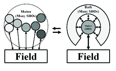
Figure 1: Equivalence of the matter-field model with many species of matter oscillators [27] and the matter-field-bath model employed here.

Consequently, a desired quantization approach for Maxwell’s equations in lossy and dispersive media requires: (1) an elegant Hamitonian with clear and significant physical meaning; (2) a rigorous quantization procedure satisfying canonical commutation relations; (3) an effective and numerically-implementable susceptibility model satisfying Kramers-Kronig relation.

Here, a lucid picture of quantum dissipation in electromagnetic system is presented to fulfill the above requirements. First, the field-matter system is quantized without mode decomposition or diagonalization of the system. Then the matter is coupled to a noise bath to induce the appearance of dissipation and Langevin sources. The choice to explicitly involve the bath is to maintain a strong connection with the classical system. To this end, we also use the quantization via the quantum Hamilton equations [40, 41]. In this work, the matter will be described by multi-species Lorentz oscillators, but only one species will be considered here. It will be evident that the multi-species generalization is straightforward.

The following emphasizes the novelty of the approach presented here:

• The work starts with a Hamiltonian from first principles. Some of the previous works started with Huttner and Barnett’s result of Fano diagonalization and polariton. But here, diagonalization of the system of equations or mode decomposition is not needed.

• This approach starts with the time-domain Hamiltonian. Frequency domain methods follow naturally from time-domain ones if the system is linear.

• Since a general heat-bath model is used, the heat-bath needs not necessary be in thermal equilibrium as in fluctuation dissipation theorem. Hence, it is possible to evolve this work along non-equilibrium calculation as in non-equilibrium Green’s function approach adopted in quantum electron transport [38, 39].

• The high-loss model is different from that of Welsch’s group. It is able to deal with high loss in quantum electromagnetics (QEM). The preservation of the commutation relations is rigorously proved which leads to the same commutation relation of current as in fluctuation dissipation theorem for both the low-loss and high-loss cases. As shall be shown, the classical Drude-Lorentz-Sommerfeld (DLS) model is not suitable for the high-loss case.

• Also, the commutation relation is shown to be satisfied in the ensemble averaging sense after introducing phenomenological loss. Furthermore, the Hamiltonian of the quantum system satisfies the energy conservation in the ensemble average sense.

Before proceeding, we would like to address a large body of recent literatures that model quantum dissipation through a cascade of two-level systems [44, ref. therein]. This approach is especially important for superconducting qubits, in which tunneling junction defects have been identified as the main cause of dissipation and decoherence. However, these defects still need to couple to phonon excitations of the junction material to cause dissipation. In such cases the oscillator model, though incomplete, is still important for gaining insights into the problem.

II Classical description of the field-matter system

The interaction of electrons or charged particles of mass $m$ with an electric field is often treated classically by the equation of motion as

$$m\overset{\bm{..}}{x}+m\gamma\overset{\bm{.}}{x}+\kappa x=qE.$$ (1)

On the left-hand-side, the first term is due to inertia since $\overset{\bm{..}}{x}$ is the acceleration of the charged particle. The second term is due to friction or collision since it is proportional to the velocity $\overset{\bm{.}}{x}$ and $\gamma$ is the collision frequency. And the third term is due to a restoring force similar to Hooke’s law with the spring constant $\kappa$. The right-hand side is the driving force due to the electric field $E$ while $q$ is the particle charge. For lack of a better name, this model will be called the DLS model since these researchers have contributed to it at various times. Sommerfeld has contributed to the quantum theory of such model.

Many models follow from this model. When the friction term dominates, the Drude model can be derived from it; when the inertia term and the spring term dominate, the above is often called a Lorentz oscillator; also, when the spring term and the friction term dominate, the Debye relaxation model follows. Furthermore, when the collision and the spring terms are absent, the effective permittivity for cold collisionless plasma can be derived. The above equation can be easily converted into a form

$$\overset{\bm{..}}{x}+\gamma\overset{\bm{.}}{x}+\omega_{0}^{2}x=qE/m.$$ (2)

where $\omega_{0}=\sqrt{\kappa/m}$ is the resonant frequency of the oscillator if loss is absent or $\gamma=0$. For the lossless case, the DLS oscillator becomes the Lorentz oscillator which is just a simple harmonic oscillator: it can be quantized.

II-A Coupling of Maxwellian Free Field to Lorentz Oscillators

The quantization of free electromagnetic fields in a lossless and dispersionless medium has recently been given using a different viewpoint without mode decompositions [40, 41]. In this work, the field-matter-bath model will be introduced. The “field” here refers to the free field or the photon field. The “matter” here will be modeled by a collection of Lorentz oscillators as in classical electromagnetics. The “bath” will be modeled by the coupling of the Lorentz oscillators to an infinite random assortment of simple harmonic oscillators which are also Lorentz oscillators. This is similar to the Hopfield model and also similar to the field-matter-bath model of Huttner and Barnett [18].

However, using a similar approach here compared to before [40, 41], the quantization of free electromagnetic fields coupled to lossless Lorentz dipoles is given without the need for mode decomposition and diagonalization of the system. As shall be shown, due to this coupling, the total field-matter system is dispersive, but lossless. Next, loss can be induced by coupling the field-matter system to a noise bath of harmonic oscillators, giving rise to a field-matter-bath system with quantum dissipation. Here, only one species of Lorentz dipoles is presented, but generalization to multiple species of Lorentz dipoles can be easily achieved so that arbitrary linear dispersive media can be modeled. In Philbin’s work [27], an integral over the frequencies for these Lorentz oscillator fields are used to connect to the electric permittivity and magnetic susceptibilities of the linear dispersive materials.

To understand the dispersion better, the Maxwellian free field can be thought of as a system where the dipoles are formed by the polarization of electron-positron (e-p) pairs lurking in vacuum [45, p. 361]. The electric flux due to these e-p pairs is given by ${{\bf D}}=\varepsilon_{0}{{\bf E}}$, and their resonant frequencies are so high that the $\varepsilon_{0}$ can be regarded as dispersionless for the free field or the photon field. In dispersive media consisting of field-matter coupling, the Maxwellian system for the free or vacuum field is coupled to Lorentz dipoles or oscillators representing the media. The Lorentz dipoles model the oscillation of charged atoms or molecules that are bulky and hence, have much larger inertial mass: They cannot be turned on (or off) instantaneously, giving rise to dispersion. Moreover, they have resonant frequencies much less than those of the e-p pairs in vacuum [46].

II-B The Classical Equations for the Coupled System

One starts with a single lossless Lorentz oscillator. A distribution of these Lorentz oscillators gives rise to polarization density, and thus, polarization current. A classical picture of this is given in many text books. For simplicity and without loss of generality, $\mu=\epsilon=1$ is assumed [47]. The polarization current can be easily derived from (2), and the pertinent equation can be written as

$$\overset{\bm{..}}{{{\bf P}}}({{\bf r}},t)+\gamma\overset{\bm{.}}{{{\bf P}}}({{\bf r}},t)+\omega_{0}^{2}{{\bf P}}({{\bf r}},t)=\omega_{p}^{2}{{\bf E}}({{\bf r}},t)$$ (3)

where ${{\bf P}}=nq{{\bf x}}$, the plasma frequency is $\omega_{p}^{2}=nq^{2}/(m\epsilon)$ where $n$ is the charge particle density and $m$ is the mass of the charged particle with the charge of $q$. Also, the normalized ${{\bf E}}$ and ${{\bf P}}$ have the same unit. Consequently, Maxwell’s equations can be augmented by coupling to the polarization current as follows.

$$\overset{\bm{.}}{{{\bf H}}}({{\bf r}},t) =-\nabla\times{{\bf E}}({{\bf r}},t)$$ (4)

$$\overset{\bm{.}}{{{\bf E}}}({{\bf r}},t) =\nabla\times{{\bf H}}({{\bf r}},t)-{{\bf V}}({{\bf r}},t)$$ (5)

where ${{\bf P}}({{\bf r}},t)$ is the polarization density, and ${{\bf V}}({{\bf r}},t)=\overset{\bm{.}}{{{\bf P}}}({{\bf r}},t)$ is the polarization current. Here, ${{\bf E}}$ and ${{\bf H}}$ are the free fields of the system. The flux ${{\bf D}}={{\bf E}}+{{\bf P}}$ in the present notation. In addition, the above implies that $\nabla\cdot{{\bf H}}({{\bf r}},t)=0$ and $\nabla\cdot{{\bf E}}({{\bf r}},t)=-\varrho_{\scriptscriptstyle P}({{\bf r}},t)$, where $\varrho_{\scriptscriptstyle P}({{\bf r}},t)=\nabla\cdot{{\bf P}}({{\bf r}},t)$, is the polarization charge. Therefore, (3) can be rewritten as two coupled first order equations in time [48]

$$\overset{\bm{.}}{{{\bf P}}}({{\bf r}},t) ={{\bf V}}({{\bf r}},t)$$ (6)

$$\overset{\bm{.}}{{{\bf V}}}({{\bf r}},t) =\omega_{p}^{2}{{\bf E}}({{\bf r}},t)-\gamma{{\bf V}}({{\bf r}},t)-\omega_{0}^{2}{{\bf P}}({{\bf r}},t)$$ (7)

Hence, the loss in the system is represented through $\gamma\neq 0$. In order to quantize the system of equations, $\gamma$ is set to zero first to model the lossless case. This gives rise to a lossless Hermitian system that can be quantized similar to before [40, 41], albeit with some complication since the medium is now dispersive. Eventually, the system will be coupled to a bath of harmonic oscillators, from which quantum dissipation follows.

II-C Lorenz Gauge and the Decoupled Potentials

As mentioned before, the lossless dispersive case will be considered first, as it is easily quantized due to the Hermitian nature of the system. To this end, one needs to derive the Hamiltonians that describe the above system. The Lorenz gauge will be used here [49], since it is commensurate with the special relativity where space and time are treated on the same footing. Therefore,

$${{\bf E}}=-\overset{\bm{.}}{{{\bf A}}}-\nabla\Phi,\qquad{{\bf H}}={{\bf B}}=\nabla\times{{\bf A}},\qquad\nabla\cdot{{\bf A}}=-\overset{\bm{.}}{\Phi}$$ (8)

Since $\mu=1$, for the free field here, ${{\bf B}}={{\bf H}}$. With these notations, one can show easily that the original equations of motion for the decoupled potential equations, derivable from the above are:

$$\nabla^{2}\Phi({{\bf r}},t) -\overset{\bm{..}}{\Phi}({{\bf r}},t)=\varrho_{\scriptscriptstyle P}({{\bf r}},t)$$ (9)

$$\nabla\times\nabla\times{{\bf A}}({{\bf r}},t)-\nabla \nabla\cdot{{\bf A}}({{\bf r}},t)+\overset{\bm{..}}{{{\bf A}}}({{\bf r}},t)={{\bf V}}({{\bf r}},t)$$ (10)

The equation of motion for the lossless Lorentz oscillator is then

$$\overset{\bm{.}}{{{\bf V}}}({{\bf r}},t)+\omega_{0}^{2}{{\bf P}}({{\bf r}},t)=\omega_{p}^{2}{{\bf E}}({{\bf r}},t)$$ (11)

In the above, one assumes that $\nabla\cdot{{\bf P}}=\varrho_{\scriptscriptstyle P}$, and hence, $\nabla\cdot{{\bf E}}=-\varrho_{\scriptscriptstyle P}$ which explains the positive sign of $\varrho_{\scriptscriptstyle P}$ on the right-hand side of (9).

II-D Derivation of the Classical Hamiltonian

In order to quantize the electromagnetic system, its classical Hamiltonian needs to be derived first. To derive the corresponding classical Hamiltonians for the different fields, conjugate momenta for ${{\bf A}}$, $\Phi$, and ${{\bf P}}$ are defined as

$$\mbox{\boldmath$\Pi$}_{A}({{\bf r}},t)=\overset{\bm{.}}{{{\bf A}}}({{\bf r}},t),\qquad\Pi_{\Phi}({{\bf r}},t)=\overset{\bm{.}}{\Phi}({{\bf r}},t),$$

$$\mbox{\boldmath$\Pi$}_{P}=\beta{{\bf V}}=\beta\overset{\bm{.}}{{{\bf P}}}({{\bf r}},t)$$ (12)

Then similar to the method outlined in [40, 41], the sources on the right-hand side of (9) to (11) can be treated as impressed sources first. Then one arrives at the Hamiltonian densities for the scalar potential, vector potential, and the polarization density. They are:

$$\mathscr{H}_{A} =\frac{1}{2}\left[\mbox{\boldmath$\Pi$}_{A}^{2}+\left(\nabla\times{{\bf A}}\right)^{2}+\left(\nabla\cdot{{\bf A}}\right)^{2}-2{{\bf A}}\cdot{{\bf V}}\right]$$ (13)

$$\mathscr{H}_{\Phi} =\frac{1}{2}\left[\Pi_{\Phi}^{2}+\left(\nabla\Phi\right)^{2}+2\Phi\varrho_{\scriptscriptstyle P}\right]$$ (14)

$$\mathscr{H}_{P} =\frac{1}{2}\left[\mbox{\boldmath$\Pi$}_{P}^{2}/\beta+f{{\bf P}}^{2}-2{{\bf P}}\cdot{{\bf E}}\right]$$ (15)

where $\beta=1/\omega_{p}^{2}$, $f=\omega_{0}^{2}/\omega_{p}^{2}$. The Hamiltonian is related to the Hamiltonian density via

$$H=\int\!dx^{4}(\mathscr{H}_{A}-\mathscr{H}_{\Phi}+\mathscr{H}_{P})$$ (16)

In the above, $dx^{4}=dtd{\bf r}$; integration over four space (space and time) is necessary since in a dispersive medium, the fields from different times affect each other. It is also implicitly implied that the above Hamiltonian densities are integrated over four space that allows the invocation of integration by parts.

It is to be noted that in (13) to (15), there exist coupling between the different Hamiltonians. The Hamiltonian for ${{\bf A}}$ has the polarization current ${{\bf V}}$ in it, while that for $\Phi$ has the polarization charge $\varrho_{\scriptscriptstyle P}$ in it, and that for ${{\bf P}}$ has ${{\bf E}}$ in it, where ${{\bf E}}$ is related to ${{\bf A}}$ and $\Phi$ via (8). But so far, the sources on the right-hand side of (9) to (11) are treated as “impressed sources” as expounded in [41]. This is incorrect as “impressed sources” cannot appear if we are writing down a Hamiltonian for the entire system, with no external influence.

To remedy this, the total Hamiltonian is the sum of the three Hamiltonians plus the interaction energy. As shall be seen, it is via the interaction energy that the coupling occurs. Hence, the corrected Hamiltonian becomes

$$H=\int\!dx^{4}(\mathscr{H}_{A}-\mathscr{H}_{\Phi}+\mathscr{H}_{P}+2{{\bf E}}\cdot{{\bf P}}-\Phi\varrho_{\scriptscriptstyle P})$$

$$=\int\!dx^{4}(\mathscr{H}_{A}-\mathscr{H}_{\Phi}+\mathscr{H}_{P}+2{{\bf A}}\cdot{{\bf V}}+\Phi\varrho_{\scriptscriptstyle P})$$ (17)

The above equality can be shown using integration by parts over space and time. It can be further shown, using integration by parts in space and time, that the ${{\bf A}}\cdot{{\bf V}}$ cancels a term in ${{\bf P}}\cdot{{\bf E}}$, leaving behind a ${{\bf P}}\cdot\nabla\Phi$ term in $\mathscr{H}_{P}$. The sum Hamiltonian then becomes

$$H= \int\!dx^{4}\,\frac{1}{2}\left[\mbox{\boldmath$\Pi$}_{A}^{2}+\left(\nabla\times{{\bf A}}\right)^{2}+\left(\nabla\cdot{{\bf A}}\right)^{2}\right.$$

$$-\left.\Pi_{\Phi}^{2}-\left(\nabla\Phi\right)^{2}+\mbox{\boldmath$\Pi$}_{P}^{2}/\beta+f{{\bf P}}^{2}+2{{\bf P}}\cdot\nabla\Phi\right]$$ (18)

It can now be shown that the above is in fact (see Appendix A)

$$H=\int\!dx^{4}\,\frac{1}{2}\left[{{\bf E}}^{2}+{{\bf H}}^{2}+\beta{{\bf V}}^{2}+f{{\bf P}}^{2}\right]$$ (19)

The above result is physically important because the first two terms correspond to energy stored in the electric and magnetic free fields, respectively; the third and the fourth terms are the kinetic and potential energies stored in the Lorentz oscillator, respectively. The above result is comforting since it implies that the Hamilton is equal to the total energy of the system: This has to be a constant of motion.

However, the equations of motion in (9) to (11) cannot be derived readily from (II-D). The reason is that as the free field is produced by the Lorentz oscillator, there is a back action of the free field onto the Lorentz oscillator. The Hamiltonians used in equations (13), (14), and (15) do not consider this back action. Therefore, when this back action is present, the conjugate momentum of ${{\bf A}}$ has to be redefined.

To this end, a new conjugate momentum for ${{\bf A}}$, namely $\mbox{\boldmath$\Pi$}_{AP}=\overset{\bm{.}}{{{\bf A}}}-{{\bf P}}$, is defined. Then (II-D) becomes [50]

$$H= \int\!d{{\bf r}}\,\frac{1}{2}\left[\left(\mbox{\boldmath$\Pi$}_{AP}+{{\bf P}}\right)^{2}+\left(\nabla\times{{\bf A}}\right)^{2}+\left(\nabla\cdot{{\bf A}}\right)^{2}\right.$$

$$-\left.\Pi_{\Phi}^{2}-\left(\nabla\Phi\right)^{2}+\mbox{\boldmath$\Pi$}_{P}^{2}/\beta+f{{\bf P}}^{2}+2{{\bf P}}\cdot\nabla\Phi\right]$$ (20)

In the above, the Hamiltonian involves now an integral over three-space since this Hamiltonian remains to be a constant of motion for an energy conserving system. Hamilton equations, similar to those given in [40, 41], can now be invoked to derive the equations of motion for the conjugate variables, namely,

$$\overset{\bm{.}}{{{\bf A}}}({{\bf r}},t) =\frac{\delta H}{\delta\mbox{\boldmath$\Pi$}_{AP}({{\bf r}},t)}, \overset{\bm{.}}{\mbox{\boldmath$\Pi$}}_{AP}({{\bf r}},t) =-\frac{\delta H}{\delta{{\bf A}}({{\bf r}},t)}$$ (21)

$$\overset{\bm{.}}{\Phi}({{\bf r}},t) =-\frac{\delta H}{\delta\Pi_{\Phi}({{\bf r}},t)}, \overset{\bm{.}}{\Pi}_{\Phi}({{\bf r}},t) =\frac{\delta H}{\delta\Phi({{\bf r}},t)}$$ (22)

$$\overset{\bm{.}}{{{\bf P}}}({{\bf r}},t) =\frac{\delta H}{\delta\mbox{\boldmath$\Pi$}_{P}({{\bf r}},t)}, \overset{\bm{.}}{\mbox{\boldmath$\Pi$}}_{P}({{\bf r}},t) =-\frac{\delta H}{\delta{{\bf P}}({{\bf r}},t)}$$ (23)

The minus sign found in the equations of motion for $\Phi$ and $\Pi_{\Phi}$ is because the total Hamiltonian is proportional to Hamiltonian for the vector potential minus the Hamiltonian for the scalar potential. This was further explained in [40, 41].

It can be shown easily that the equations of motion  (9), (10), (11), can be re-derived from the above. The above gives the classical Hamiltonian description of the system. Once the classical Hamiltonian description of the system is available, the quantum Hamiltonian description of the system can be arrived at. But since such exercise is infrequent, the procedure will be further elaborated next. The left column above corresponds to the equations of motion for ${{\bf A}}$, $\Phi$ and ${{\bf P}}$. They correspond to taking the variation of the Hamiltonian with respect to the conjugate momenta $\mbox{\boldmath$\Pi$}_{AP}$, $\Pi_{\Phi}$, and ${{\bf V}}$, and they can be easily done. Therefore, evaluating the right-hand sides of all the above equations by taking the proper functional derivatives of the Hamiltonian, one arrives at 6 equations

$$\overset{\bm{.}}{{{\bf A}}}({{\bf r}},t) =\mbox{\boldmath$\Pi$}_{AP}({{\bf r}},t)+{{\bf P}}({{\bf r}},t),$$

$$\overset{\bm{.}}{\mbox{\boldmath$\Pi$}}_{AP}({{\bf r}},t) =-\nabla\times\nabla\times{{\bf A}}({{\bf r}},t)+\nabla\nabla\cdot{{\bf A}}({{\bf r}},t)$$ (24)

$$\overset{\bm{.}}{\Phi}({{\bf r}},t) =\Pi_{\Phi}({{\bf r}},t)$$

$$\overset{\bm{.}}{\Pi}_{\Phi}({{\bf r}},t) =\nabla^{2}\Phi-\varrho_{\scriptscriptstyle P}$$ (25)

$$\overset{\bm{.}}{{{\bf P}}}({{\bf r}},t) =\mbox{\boldmath$\Pi$}_{P}({{\bf r}},t)/\beta={{\bf V}}({{\bf r}},t),$$

$$\beta\overset{\bm{.}}{{{\bf V}}}({{\bf r}},t) =-f{{\bf P}}({{\bf r}},t)-\mbox{\boldmath$\Pi$}_{AP}({{\bf r}},t)-\nabla\Phi({{\bf r}},t)-{{\bf P}}({{\bf r}},t)$$

$$=-f{{\bf P}}({{\bf r}},t)+{{\bf E}}({{\bf r}},t)$$ (26)

The equations above contain the equations of motion for the original variables, ${{\bf A}}$, $\Phi$, and ${{\bf P}}$, and the conjugate variables $\mbox{\boldmath$\Pi$}_{AP}$, $\Pi_{\Phi}$, and ${{\bf V}}$. They can be combined to yield the classical equations of motion in (9) to (11). It is to be reminded that when functional derivatives in (21) to (23) are taken, they yield Dirac delta functions with the sifting property similar to the rule expounded in [40]. Examples of which are

$$\frac{\delta{{\bf A}}({{\bf r}},t)}{\delta{{\bf A}}({{\bf r}}^{\prime},t)}=\frac{\delta\mbox{\boldmath$\Pi$}({{\bf r}},t)}{\delta\mbox{\boldmath$\Pi$}({{\bf r}}^{\prime},t)}={{\bf\overline{I}}}\delta({{\bf r}}-{{\bf r}}^{\prime}),$$ (27)

$$\frac{\delta{{\bf A}}({{\bf r}},t)}{\delta\mbox{\boldmath$\Pi$}({{\bf r}}^{\prime},t)}=\frac{\delta\mbox{\boldmath$\Pi$}({{\bf r}},t)}{\delta{{\bf A}}({{\bf r}}^{\prime},t)}=0$$ (28)

Their use greatly simplifies the integral of the Hamiltonian.

It is pleasing to note that the equations of motion of the total field-matter system: Maxwellian free fields coupled to the Lorentz oscillators can be expressed in terms of Hamilton equations of motion. This is definitely a more complicated system than that for the Maxwellian free fields alone. Although the Coulomb gauge which quantizes only the transverse fields is widely used in quantum optics, we would like to present a different quantization approach under the Lorenz gauge in this work. In view of gauge invariance and the numerical niceties of the Lorenz gauge, we feel that this scheme should be considered as an alternative which may present more choices when integrating the capabilities of computational electromagnetics with quantum optics [42].

III Quantum description of the field-matter system

To arrive at the quantum equations of motion, first, the quantum Hamiltonian corresponding to the above has to be derived. Hence, to arrive at the quantum equivalence of the above classical system, it is necessary to first elevate all the conjugate variables to become quantum operators. With this, the Hamiltonian becomes an operator as well, and is now governed by

$$\hat{H}= \int\!d{\bf r}\,\frac{1}{2}\left[\left(\hat{\mbox{\boldmath$\Pi$}}_{AP}+\hat{{{\bf P}}}\right)^{2}+\left(\nabla\times\hat{{{\bf A}}}\right)^{2}+\left(\nabla\cdot\hat{{{\bf A}}}\right)^{2}\right.$$

$$\left.-\hat{\Pi}_{\Phi}^{2}-\left(\nabla\hat{\Phi}\right)^{2}+\hat{\mbox{\boldmath$\Pi$}}_{P}^{2}/\beta+f\hat{{{\bf P}}}^{2}+2\hat{{{\bf P}}}\cdot\nabla\hat{\Phi}\right]$$ (29)

These quantum operators corresponding to the conjugate variables operate on a quantum state $|\psi\rangle$ and the time evolution of the entire quantum system described by $\hat{H}$ is now given by [51]

$$\hat{H}|\psi\rangle=i\hbar\partial_{t}|\psi\rangle$$ (30)

The time evolution of each operator in this quantum system is given by the Heisenberg equation of motion:

$$i\hbar\overset{\bm{.}}{\hat{O}}=\left[\hat{O},\hat{H}\right]$$ (31)

It turns out that the quantum Hamilton equations can be derived from the above [40, 41, 43]. To this end, it is necessary that one defines the commutation relations between operators that are conjugate to each other. They are important for energy conservation. Hence, the commutation relations that should be introduced here are: [52]

$${\left[\hat{{{\bf\Pi}}}_{AP}({{\bf r}},t),\hat{{{\bf A}}}({{\bf r}}^{\prime},t)\right]}=-i\hbar\delta({{\bf r}}-{{\bf r}}^{\prime})\hat{{{\bf\overline{I}}}}$$ (32)

$${\left[\hat{\Pi}_{\Phi}({{\bf r}},t),\hat{\Phi}({{\bf r}}^{\prime},t)\right]}=+i\hbar\delta({{\bf r}}-{{\bf r}}^{\prime})\hat{I}$$ (33)

$${\left[\hat{\mbox{\boldmath$\Pi$}}_{P}({{\bf r}},t),\hat{{{\bf P}}}({{\bf r}}^{\prime},t)\right]}=-i\hbar\delta({{\bf r}}-{{\bf r}}^{\prime})\hat{{{\bf\overline{I}}}}$$ (34)

Since the variables ${{\bf A}}$, $\Phi$, and ${{\bf P}}$ are independent variables so are their conjugate variables, when elevated to be quantum operators, they are also mutually commuting. The above commutators for the fields are similar and analogous in spirit to the position-momentum commutator

$${\left[\hat{q}_{i}(t),\hat{p}_{j}(t)\right]}=i\hbar\hat{I}\delta_{ij}$$ (35)

The above commutator in (35) induces the derivative operators that can be used to abbreviate the Heisenberg equation of motion as shown previously [40, 41, 43]. Namely, in the discrete case, they are

$${\left[\hat{p}_{i^{\prime}},\hat{q}_{i}^{n}\right]} =-in\delta_{ii^{\prime}}\hat{q}_{i}^{n-1}\hbar=-i\hbar\frac{\partial}{\partial\hat{q}_{i^{\prime}}}\hat{q}_{i}^{n}$$

$${\left[\hat{p}_{i^{\prime}},\hat{H}\right]} =-i\hbar\frac{\partial}{\partial\hat{q}_{i^{\prime}}}\hat{H}=i\hbar\overset{\bm{.}}{\hat{p}}_{i^{\prime}}(t)$$ (36)

$${\left[\hat{q}_{i^{\prime}},\hat{p}_{i}^{n}\right]} =in\delta_{ii^{\prime}}\hat{p}_{i}^{n-1}\hbar=i\hbar\frac{\partial}{\partial\hat{p}_{i^{\prime}}}\hat{p}_{i}^{n}$$

$${\left[\hat{q}_{i^{\prime}},\hat{H}\right]} =i\hbar\frac{\partial}{\partial\hat{p}_{i^{\prime}}}\hat{H}=i\hbar\overset{\bm{.}}{\hat{q}}_{i^{\prime}}(t)$$ (37)

For the continuum case, the above commutators, (32) to (34) induce functional derivative operations [40, 41]. Consequently, the quantum Hamilton equations of motion are

$${\left[\hat{\mbox{\boldmath$\Pi$}}_{AP}({{\bf r}},t),\hat{H}\right]} =-i\hbar\,\frac{\delta{\hat{H}}}{\delta\hat{{{\bf A}}}({{\bf r}},t)}=i\hbar\overset{\bm{.}}{\hat{\mbox{\boldmath$\Pi$}}}_{AP}({{\bf r}},t)$$ (38)

$${\left[\hat{{{\bf A}}}({{\bf r}},t),\hat{H}\right]} =i\hbar\,\frac{\delta\hat{H}}{\delta\hat{\mbox{\boldmath$\Pi$}}_{AP}({{\bf r}},t)}=i\hbar\,\overset{\bm{.}}{\hat{{{\bf A}}}}({{\bf r}},t)$$ (39)

$${\left[\hat{\Pi}_{\Phi}({{\bf r}},t),\hat{H}\right]} =i\hbar\,\frac{\delta\hat{H}}{\delta{\hat{\Phi}}({{\bf r}},t)}=i\hbar\,\overset{\bm{.}}{\hat{\Pi}}_{\Phi}({{\bf r}},t)$$ (40)

$${\left[\hat{\Phi}({{\bf r}},t),\hat{H}\right]} =-i\hbar\,\frac{\delta\hat{H}}{\delta\hat{\Pi}_{\Phi}({{\bf r}},t)}=i\hbar\overset{\bm{.}}{\hat{\Phi}}({{\bf r}},t)$$ (41)

$${\left[\hat{\mbox{\boldmath$\Pi$}}_{P}({{\bf r}},t),\hat{H}\right]} =-i{\hbar}\,\frac{\delta{\hat{H}}}{\delta\hat{{{\bf P}}}({{\bf r}},t)}=i\hbar\,\overset{\bm{.}}{\hat{{{\bf\Pi}}}}_{P}({{\bf r}},t)$$ (42)

$${\left[\hat{{{\bf P}}}({{\bf r}},t),\hat{H}\right]} =i{\hbar}\,\frac{\delta\hat{H}}{\delta\hat{\mbox{\boldmath$\Pi$}}_{P}({{\bf r}},t)}=i\hbar\,\overset{\bm{.}}{\hat{{{\bf P}}}}({{\bf r}},t)$$ (43)

The above quantum Hamilton equations are very similar to their classical counterparts in (21) to (23), and then in (II-D) to (II-D). Hence, the quantum analogues of (9)-(11) can be obtained as in previous work [40, 41]. From them, the equations of motion of the quantum operators that are the analog of (3) to (5) for the lossless case are

$$\overset{\bm{..}}{\hat{{{\bf P}}}}({{\bf r}},t) +\omega_{0}^{2}\hat{{{\bf P}}}({{\bf r}},t)=\omega_{p}^{2}\hat{{{\bf E}}}({{\bf r}},t)$$ (44)

$$\overset{\bm{.}}{\hat{{{\bf H}}}}({{\bf r}},t) =-\nabla\times\hat{{{\bf E}}}({{\bf r}},t)$$ (45)

$$\overset{\bm{.}}{\hat{{{\bf E}}}}({{\bf r}},t) =\nabla\times\hat{{{\bf H}}}({{\bf r}},t)-\hat{{{\bf V}}}({{\bf r}},t)$$ (46)

It is to be noted that the above equations of motion of these quantum operators have meaning only if they operate on a quantum state $|\psi\rangle$ of the system. Also, the above quantum equations are derived without the normal mode decomposition approach, but can be derived directly from the Hamiltonian using the quantum Hamilton equations. Hence, diagonalization of the system is not necessary. Normal mode decomposition is possible for all linear systems in theory, but for some practical systems, they have to be done numerically. This quantization approach here avoids having to find the normal modes of the system.

III-A Preservation of Commutators

It can be shown that the commutators in (32) to (34) are still preserved with the above quantization procedure. For instance, for the commutator

$$\hat{{{\bf C}}}_{A}=\left[{{\hat{\mbox{\boldmath$\Pi$}}_{AP}}},{\hat{{{\bf A}}}}\right]$$ (47)

then,

$$\frac{d}{dt}\hat{{{\bf C}}}_{A} =\left[{\overset{\bm{.}}{\hat{\mbox{\boldmath$\Pi$}}}_{AP}},\hat{{{\bf A}}}\right]+\left[{\hat{\mbox{\boldmath$\Pi$}}_{AP}},{\overset{\bm{.}}{\hat{{{\bf A}}}}}\right]$$

$$=\left[-\nabla\times\nabla\times\hat{{{\bf A}}}+\nabla\nabla\cdot\hat{{{\bf A}}},\hat{{{\bf A}}}\right]+\left[\overset{\bm{.}}{\hat{{{\bf A}}}}-\hat{{{\bf P}}},\overset{\bm{.}}{\hat{{{\bf A}}}}\right]$$

$$=0$$ (48)

The right-hand side is zero because it can be shown that by using the discrete version of a field as expounded in [40], the space derivative of a field operator commutes with the field operator itself. Also, $\hat{{{\bf P}}}$ and $\overset{\bm{.}}{\hat{{{\bf A}}}}$ commute because ${{\bf P}}$ and $\overset{\bm{.}}{{{\bf A}}}$ are independent variables. Similar method can be used to show that the rest of the commutators in (32) to (34) are preserved in this quantization scheme. The preservation of commutators is related to the conservation of energy.

IV Dissipation by Coupling to a Noise Bath

The topic of quantum dissipation in quantum optics has been reported in many books [4, 5, 6, 7, 8, 9, 10, 11, 12, 13, 14, 15]. In this section, the coupling of a single Lorentz harmonic oscillator to a noise bath will be demonstrated. Both classical and quantum dissipations can be induced by coupling the non-dissipative system to a noise bath of harmonic oscillators [3, 18]. In classical problems, the loss in the DLS oscillator is due to the collisions of electrons with the lattice or the ions. Hence, it is reasonable to assume that the loss introduced to the Lorentz oscillator comes from its coupling to other systems which can be modeled as a noise bath.

In general, there are many sources of noise in a system. To simplify, the noise bath will be assumed to consist only of a large collection of simple harmonic oscillators. This model has been assumed in the Huttner and Barnett model [18] as well as in other quantum systems [3, 25, 27]. There in [18], the free-field is coupled to matter, and then the matter is coupled to a noise bath. The matter there is equivalent to the Lorentz oscillator here. Because of the simplification of the noise bath model, the noise bath is only modeled phenomenologically.

Hence, in this work, it is assumed that the loss in the DLS oscillator is a consequence of coupling of a Lorentz oscillator to a noise bath which is modeled by a collection of harmonic oscillators.

IV-A Classical Case

First, the classical Hamiltonian due to the coupling of the field-matter to a noise bath will be illustrated. To this end, the total Hamiltonian density is given by

$$\mathscr{H}_{PB}=\mathscr{H}_{P}+\mathscr{H}_{B}+\mathscr{H}_{INT}$$ (49)

where on the right-hand side, the first Hamiltonian density, $\mathscr{H}_{P}$, is due to matter consisting of Lorentz oscillators which are used to describe the polarization current, the second Hamiltonian density, $\mathscr{H}_{B}$, is due to the noise bath, while the third Hamiltonian density is the interaction between the matter and the bath. The Hamiltonian density $\mathscr{H}_{P}$ is as before, and reproduced here as:

$$\mathscr{H}_{P}=\frac{1}{2}\left[\beta{{{\bf V}}}^{2}+f{{{\bf P}}}^{2}+2{{{\bf P}}}\cdot{{{\bf E}}}\right]$$ (50)

The bath Hamiltonian consisting of a large random assortment of simple harmonic oscillators can be written as [53]

$$\mathscr{H}_{B}=\sum_{j}\frac{1}{2}\left[\mbox{\boldmath$\Pi$}_{P,j}^{2}/\beta_{j}+f_{j}{{\bf P}}_{j}^{2}\right]$$ (51)

where $\mbox{\boldmath$\Pi$}_{P,j}=\beta_{j}{{\bf V}}_{j}$ is the conjugate variable to ${{\bf P}}_{j}$. The interaction Hamiltonian is

$$\mathscr{H}_{INT}=\sum_{j}\left[\alpha_{j}^{\Pi}\mbox{\boldmath$\Pi$}_{P,j}\cdot\mbox{\boldmath$\Pi$}_{P}+\alpha_{j}^{P}{{\bf P}}_{j}\cdot{{\bf P}}\right]$$ (52)

The above is motivated by the discrete case: If one has $N$ discrete oscillators, coupled by a stiffness matrix $K_{ij}$, the coupling term yielding the potential energy is proportional to $\sum_{i,j}q_{i}K_{ij}q_{j}$. Similar argument can be made for coupling via the mass matrix [40, 54].

The matter-bath Hamiltonian $H_{PB}$ can be obtained by integrating the Hamiltonian density in (49) over space. The equations of motion can then be derived such that

$$\overset{\bm{.}}{{{\bf P}}}({{\bf r}},t)=\frac{\delta H_{PB}}{\delta\mbox{\boldmath$\Pi$}_{P}({{\bf r}},t)}= {{\bf V}}({{\bf r}},t)+\sum_{j}\alpha_{j}^{\Pi}\mbox{\boldmath$\Pi$}_{P,j}({{\bf r}},t)$$ (53)

$$\overset{\bm{.}}{\mbox{\boldmath$\Pi$}}_{P}({{\bf r}},t)=-\frac{\delta H_{PB}}{\delta{{\bf P}}({{\bf r}},t)}= -f{{\bf P}}({{\bf r}},t)+{{\bf E}}({{\bf r}},t)$$

$$-\sum_{j}\alpha_{j}^{P}{{\bf P}}_{j}({{\bf r}},t)$$ (54)

$$\overset{\bm{.}}{{{\bf P}}}_{j}({{\bf r}},t)=\frac{\delta H_{PB}}{\delta\mbox{\boldmath$\Pi$}_{P,j}({{\bf r}},t)}= {{\bf V}}_{j}({{\bf r}},t)+\alpha_{j}^{\Pi}\mbox{\boldmath$\Pi$}_{P}({{\bf r}},t)$$ (55)

$$\overset{\bm{.}}{\mbox{\boldmath$\Pi$}}_{P,j}({{\bf r}},t)=-\frac{\delta H_{PB}}{\delta{{\bf P}}_{j}({{\bf r}},t)}= -f_{j}{{\bf P}}_{j}({{\bf r}},t)-\alpha_{j}^{P}{{\bf P}}({{\bf r}},t)$$ (56)

It is to be noted that in the last equation above, the equation of motion for the noise bath oscillator is only coupled to the polarization current ${{\bf P}}({{\bf r}},t)$. This is unlike (IV-A) above or (II-D), where the equation of motion for the polarization current is coupled to the driving field ${{\bf E}}({{\bf r}},t)$.

IV-B Quantum Case

The derivation of the equations of motion for the quantum case is quite routine: First, the conjugate variable pairs are elevated to be operators, and then commutators between them are defined. The new commutator needed here for the bath oscillators is

$${\left[\hat{\mbox{\boldmath$\Pi$}}_{P,j}({{\bf r}},t),\hat{{{\bf P}}}_{j^{\prime}}({{\bf r}}^{\prime},t)\right]}=-i\hbar\delta({{\bf r}}-{{\bf r}}^{\prime})\delta_{jj^{\prime}}\hat{{{\bf\overline{I}}}}$$ (57)

The relevant Hamiltonian is hence elevated to be an operator. Using the quantum Hamilton equations, the equations of motion can be derived for the matter-bath coupling to be

$$\overset{\bm{.}}{\hat{{{\bf P}}}}({{\bf r}},t)=\frac{\delta\hat{H}}{\delta\hat{\mbox{\boldmath$\Pi$}}_{P}({{\bf r}},t)}=\hat{{{\bf V}}}({{\bf r}},t)+\sum_{j}\alpha_{j}^{\Pi}\hat{\mbox{\boldmath$\Pi$}}_{P,j}({{\bf r}},t)$$ (58)

$$\overset{\bm{.}}{\hat{\mbox{\boldmath$\Pi$}}}_{P}({{\bf r}},t)=-\frac{\delta\hat{H}}{\delta\hat{{{\bf P}}}({{\bf r}},t)}= -f\hat{{{\bf P}}}({{\bf r}},t)+\hat{{{\bf E}}}({{\bf r}},t)$$

$$-\sum_{j}\alpha_{j}^{P}\hat{{{\bf P}}}_{j}({{\bf r}},t)$$ (59)

$$\overset{\bm{.}}{\hat{{{\bf P}}}}_{j}({{\bf r}},t)=\frac{\delta\hat{H}}{\delta\hat{\mbox{\boldmath$\Pi$}}_{P,j}({{\bf r}},t)}=\hat{{{\bf V}}}_{j}({{\bf r}},t)+\alpha_{j}^{\Pi}\hat{\mbox{\boldmath$\Pi$}}_{P}({{\bf r}},t)$$ (60)

$$\overset{\bm{.}}{\hat{\mbox{\boldmath$\Pi$}}}_{P,j}({{\bf r}},t)=-\frac{\delta\hat{H}}{\delta\hat{{{\bf P}}}_{j}({{\bf r}},t)}=-f_{j}\hat{{{\bf P}}}_{j}({{\bf r}},t)-\alpha_{j}^{P}\hat{{{\bf P}}}({{\bf r}},t)$$ (61)

Similar to before, it is easy to show that these commutators in (34) and (57) are preserved by the above equations of motion.

IV-C Asymptotic Solution–Coupling of the Lorentz Oscillator to a Noise Bath

The above coupled equations of motion has no closed form or analytic solution. But in the limit when the bath is assumed to be infinitely large, approximate analytic solution can be obtained. Before this is shown, it is necessary to simplify the above equations of motion. A closer look at the equations of motion shows that they are entirely local: Namely, the Lorentz oscillators are not mutually coupled to each others, unlike the e-p pair oscillators in Maxwell’s equations. Moreover, the ($x$, $y$, $z$) components of the oscillations are entirely independent of each other. Therefore, they can be fully described by scalar oscillators at a given location. This is also the spirit of the matter-bath model in works of other researchers [18, 25, 27].

Consequently, the matter-bath model can be understood by studying only one single oscillator’s coupling to a noise bath. (Only the driving field ${{\bf E}}({{\bf r}},t)$ is a function of position.) To this end, the above problem will be reduced to one involving a single harmonic oscillator coupled to a noise bath. Therefore, the following replacements are assumed next:

$$\hbar\omega_{0}\hat{\zeta}^{2}\leftrightarrow f\hat{{{\bf P}}}^{2},\qquad\hbar\omega_{0}\hat{\pi}^{2}\leftrightarrow\beta\hat{{{\bf V}}}^{2},$$

$$\hbar\omega_{j}\hat{\zeta}_{j}^{2}\leftrightarrow f_{j}\hat{{{\bf P}}}_{j}^{2},\qquad\hbar\omega_{j}\hat{\pi}_{j}^{2}\leftrightarrow\beta_{j}\hat{{{\bf V}}}_{j}^{2}$$ (62)

Then the Hamiltonian for a single Lorentz oscillator coupled to a noise bath becomes

$${\hat{H}}_{PB}= \frac{1}{2}\hbar\omega_{0}\left(\hat{\pi}^{2}+\hat{\zeta}^{2}\right)+\frac{1}{2}\hbar\sum_{j}\omega_{j}\left(\hat{\pi_{j}}^{2}+\hat{\zeta_{j}}^{2}\right)$$

$$+\sum_{j}\hbar\left(\alpha_{j}^{\zeta}\hat{\zeta}\hat{\zeta}_{j}+\alpha_{j}^{\pi}\hat{\pi}\hat{\pi}_{j}\right)+2C\hat{\zeta}\hat{E}$$ (63)

The first term represents the Hamiltonian for the single Lorentz oscillator yielding the polarization current inside the medium, while the second term represents the Hamiltonian of the harmonic oscillators in the bath. The third term is the interaction of the single Lorentz oscillator with the bath oscillators. The last term can be ignored for the following analyses. Because the matter is coupled to the noise bath only and $E$ can be regarded as the external driving field. In this model, the Lorentz oscillator and the noise oscillators at different locations are completely independent of each other, hence, $\omega_{0}$, $\omega_{j}$, $\alpha_{j}^{\zeta}$, $\alpha_{j}^{\pi}$, $C$, and $\hat{E}$ can be functions of positions. In (IV-C), these equations are similar to those of the mode decomposition picture [41], but they represent modes at different locations.

Without the last term, the above Hamiltonian is that of a collection of $N$ coupled simple harmonic oscillators. They will have $N$ natural modes or resonant frequencies. The number of modes will become infinitely large as $N\rightarrow\infty$. Moreover, since this is a lossless Hermitian system, all the resonant frequencies are real. But when the system is separated into a single Lorentz oscillator coupled to a bath of harmonic oscillators, one can discern energy flow from the Lorentz oscillator to the bath as shall be shown by the following analysis. One can show that the natural mode of the “lossy” Lorentz (DLS) oscillator becomes complex implying that the natural mode decays with time. To find the natural modes of the coupled harmonic oscillators, the driving term or the last term in the Hamiltonian in (IV-C) can be ignored.

To this end, one can then transform the above into normal variables [4] by letting

$$\hat{\zeta}=\frac{1}{\sqrt{2}}\left(\hat{a}+\hat{a}^{\dagger}\right),\quad\hat{\pi}=\frac{1}{i\sqrt{2}}\left(\hat{a}-\hat{a}^{\dagger}\right),$$

$$\hat{\zeta}_{j}=\frac{1}{\sqrt{2}}\left(\hat{b}_{j}+\hat{b}_{j}^{\dagger}\right),\quad\hat{\pi}_{j}=\frac{1}{i\sqrt{2}}\left(\hat{b}_{j}-\hat{b}_{j}^{\dagger}\right)$$ (64)

where $\hat{a}$ and $\hat{b}_{j}$ represent the modes of the single Lorentz oscillator and the $j$-th bath oscillator, respectively. Consequently, the Hamiltonian becomes

$${\hat{H}}_{PB}= \frac{1}{2}\hbar\omega_{0}\left(\hat{a}\hat{a}^{\dagger}+\hat{a}^{\dagger}\hat{a}\right)+\sum_{j}\frac{1}{2}\hbar\omega_{j}\left(\hat{b}_{j}\hat{b}_{j}^{\dagger}+\hat{b}_{j}^{\dagger}\hat{b}_{j}\right)$$

$$+\sum_{j}\hbar\frac{\alpha_{j}^{\zeta}+\alpha_{j}^{\pi}}{\sqrt{2}}\left(\hat{a}\hat{b}_{j}^{\dagger}+\hat{a}^{\dagger}\hat{b}_{j}\right)$$

$$+\sum_{j}\hbar\frac{\alpha_{j}^{\zeta}-\alpha_{j}^{\pi}}{\sqrt{2}}\left(\hat{a}\hat{b}_{j}+\hat{a}^{\dagger}\hat{b}_{j}^{\dagger}\right)$$ (65)

If $\alpha^{\zeta}_{j}=\alpha^{\pi}_{j}$, then the last term above vanishes; or one can make the rotating wave approximation that the last term is rapidly varying, and hence, its contribution to the total Hamiltonian is small. Therefore, the final Hamiltonian becomes

$${\hat{H}}_{PB}= \frac{1}{2}\hbar\omega_{0}\left(\hat{a}\hat{a}^{\dagger}+\hat{a}^{\dagger}\hat{a}\right)+\sum_{j}\frac{1}{2}\hbar\omega_{j}\left(\hat{b}_{j}\hat{b}_{j}^{\dagger}+\hat{b}_{j}^{\dagger}\hat{b}_{j}\right)$$

$$+\sum_{j}\tilde{\gamma}_{j}\hbar\left(\hat{a}\hat{b}_{j}^{\dagger}+\hat{a}^{\dagger}\hat{b}_{j}\right)$$ (66)

where $\tilde{\gamma}_{j}=\frac{\alpha_{j}^{\zeta}+\alpha_{j}^{\pi}}{\sqrt{2}}$. The equations of motion for $\hat{a}$ and $\hat{b}_{j}$ can be easily derived using the Heisenberg equation of motion  or

$$\overset{\bm{.}}{\hat{a}}=\frac{1}{i\hbar}\left[\hat{a},\hat{H}\right],\qquad\overset{\bm{.}}{\hat{b}_{j}}=\frac{1}{i\hbar}\left[\hat{b}_{j},\hat{H}\right]$$ (67)

They become [47]

$$\overset{\bm{.}}{\hat{a}} =-i\left(\omega_{0}\hat{a}+\sum_{j}\tilde{\gamma}_{j}\hat{b}_{j}\right)$$ (68)

$$\overset{\bm{.}}{\hat{b}}_{j} =-i\left(\omega_{j}\hat{b}_{j}+\tilde{\gamma}_{j}\hat{a}\right)$$ (69)

The above is a Hermitian system with no loss. The corresponding eigenmodes of the system correspond to lossless time-harmonic oscillators of a Hermitian system. If there are $N$ oscillators coupled together, there would be $N$ degrees of freedom and this system of equations yields $N$ modes. These equations account for the coupling of the single Lorentz oscillator to the noise bath oscillators, but not the coupling between the oscillators within the noise bath.

However, if the initial condition is such that the starting states of the harmonic oscillators in the bath are completely random, it has been shown in [7, eq. (6.89)], [10] and [55] that the leakage of energy from the single oscillator to the bath gives rise to the decay of the amplitude of the harmonic oscillator.

Following [10] by defining $\hat{b}_{j}=\hat{\tilde{b}}_{j}e^{-i\omega_{j}t}$, the second equation can be simplified as

$$\overset{\bm{.}}{\hat{\tilde{b}}}_{j}=-i\tilde{\gamma}_{j}\hat{a}e^{i\omega_{j}t}$$ (70)

The above equation can be integrated to yield

$$\hat{\tilde{b}}_{j}(t)=-i\int_{0}^{t}\tilde{\gamma}_{j}\hat{a}(\tau)e^{i\omega_{j}\tau}d\tau+\hat{\tilde{b}}_{j}(0)$$ (71)

Upon substituting the above into equation (68), and exchanging the order of integration and summation, one arrives at

$$\overset{\bm{.}}{\hat{a}}= -i\omega_{0}\hat{a}-\int_{0}^{t}\sum_{j}\tilde{\gamma}_{j}^{2}\hat{a}(\tau)e^{-i\omega_{j}(t-\tau)}d\tau$$

$$-i\sum_{j}\tilde{\gamma}_{j}\hat{\tilde{b}}_{j}(0)e^{-i\omega_{j}t}$$ (72)

The above can be thought of as a model for detailed balance, but it has no closed-form expression for the terms. So to obtain approximate analytic expressions for the terms, one can study the summation terms inside the second term on the right-hand side in greater detail. The summation above is given by

$$\sum_{j}\tilde{\gamma}_{j}^{2}e^{-i\omega_{j}(t-\tau)}$$ (73)

It clearly peaks when $t=\tau$. Moreover, if one assumes that $\gamma_{j}$ is weakly dependent on $j$ so that it can be approximated by $\tilde{\gamma}_{j}^{2}\approx\frac{\eta}{2\pi}\Delta\omega$ then

$$\sum_{j}\tilde{\gamma}_{j}^{2}e^{-i\omega_{j}(t-\tau)}\approx\frac{\eta}{2\pi}\int_{-\infty}^{\infty}e^{-i\omega(t-\tau)}d\omega=\eta\delta(t-\tau)$$ (74)

The above equation now becomes

$$\overset{\bm{.}}{\hat{a}}=-i\omega_{0}\hat{a}-\eta\hat{a}-i\sum_{j}\tilde{\gamma}_{j}\hat{\tilde{b}}_{j}(0)e^{-i\omega_{j}t}$$ (75)

which is the same as that derived by the Laplace transform method in the Appendix as $\hat{\tilde{b}}_{j}(0)=\hat{b}_{j}(0)$. It is interesting to note that the coupling to the bath introduces a dissipation term given by $-\eta\hat{a}$, but it is also augmented by a source term given by the last term above. The augmented source term can be regarded as the Langevin source. In Figure 2, the coupled system is sketched.

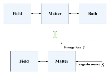
Figure 2: The field-matter-bath coupled system. The effect of the bath is the introduction of loss and Langevin sources into the matter system, which further influences the field.

V Physical Interpretation

One can explain the physical meaning of the above further. Equations (68) and (69), represent a Hermitian lossless system of coupled oscillating modes. All the resonant modes of the Hermitian system can be proved to be real. However, the second term on the right-hand side of (68) implies that $\hat{a}$ is being driven by $\hat{b}_{j}$. But $\hat{b}_{j}$ is being also bring driven by $\hat{a}$: this point is being expressed by (71). The first term on the right-hand side represents the back action by $\hat{a}$ on $\hat{b}_{j}$, while the second term implies that $\hat{b}_{j}$ will remain unchanged if $\hat{a}$ and $\hat{b}_{j}$ are not coupled together.

In (IV-C), the second term on the right-hand side can be written as a convolutional integral:

$$\hat{a}(t)\circledast B(t)$$ (76)

where $B(t)=\sum_{j}\tilde{\gamma}_{j}^{2}e^{-i\omega_{j}t}$. It is seen that $B(t)$ is the sum of many oscillators with different frequencies. This term eventually leads to the loss term in (75), but the loss is caused by the destructive interference or non-time-reversibility of the oscillators in the bath. That it becomes a loss term that “siphons” energy from the oscillator to the bath is only valid in the ensemble average sense. The last term in (75), on the other hand, “pumps” energy back into the $\hat{a}$ oscillator. But it is seen that the last term is again a sum of incoherent oscillators with initial values $\hat{b}_{j}(0)$ which is random.

The initial value $\hat{b}_{j}(0)$ is very much related to the temperature of the noise bath: The higher the temperature, the larger the initial values. Also, this term is “white” (as in white noise) compared to the term that siphons energy off the $\hat{a}$ oscillator. By energy conservation, at thermal equilibrium, these two energies, siphoned energy and pumped energy, should be equal to each other, but they are equal only in the ensemble average sense.

Because of this physical interpretation, the last term in (75) can be expressed as the Langevin noise source, namely,

$$\overset{\bm{.}}{\hat{a}}=-i\omega_{0}\hat{a}-\eta\hat{a}+\hat{F}(t)$$ (77)

where

$$\hat{F}(t)=-i\sum_{j}\tilde{\gamma}_{j}\hat{b}_{j}(0)e^{-i\omega_{j}t}$$ (78)

By the same token, the creation operator equivalence of the above is

$$\overset{\bm{.}}{\hat{a}}^{\dagger}=i\omega_{0}\hat{a}^{\dagger}-\eta\hat{a}^{\dagger}+\hat{F}^{\dagger}(t)$$ (79)

The above system cannot be proven to be Hermitian, but it has descended from a Hermitian system with asymptotic approximations. So it should be quasi-Hermitian, or Hermitian in the average sense. Or one can envision that the Langevin sources produce a response that compensates the loss due to coupling of the system to the noise bath. This is similar in spirit to the fluctuation dissipation theorem [56, 57, 31] where the loss of energy from the system to the noise bath in thermal equilibrium is compensated by the back-coupling of energy back from the noise bath to the system.

Furthermore, it can be shown that the Langevin sources are highly uncorrelated in time such that [7, 10]

$$\langle[\hat{F}(t),\hat{F}^{\dagger}(t^{\prime})]\rangle =\sum_{j}|\gamma_{j}|^{2}e^{i\omega_{j}(t^{\prime}-t)}\langle[\hat{b}_{j}(0),\hat{b}_{j}^{\dagger}(0)]\rangle$$

$$=2\eta\delta(t-t^{\prime})$$ (80)

where the angular bracket implies ensemble average. And more importantly, the commutator between the $\hat{a}$ and $\hat{a}^{\dagger}$ is preserved, as it was in the original Hermitian system. The real and imaginary parts of operators $\hat{a}$ and $\hat{a}^{\dagger}$ are related to the quantum observables $\hat{p}$ and $\hat{q}$. The commutator of $\hat{p}$ and $\hat{q}$ is related to the commutator of $\hat{a}$ and $\hat{a}^{\dagger}$. As has been seen before, these commutators are important for inducing the quantum Hamilton equations of motion. The loss of these commutators would have meant that the quantum equations of motion are not preserved. It also means that energy is not conserved. This would have been bizzare, as it means that physical laws are not preserved.

One can define a Langevin noise operator such that

$$\hat{F}(t)=\sqrt{2\eta}\hat{f}(t)$$ (81)

then

$$\left[\hat{f}(t),\hat{f}^{\dagger}(t^{\prime})\right]=\delta(t-t^{\prime})$$ (82)

implying that the Langevin source is “white”.

Some further remarks are in order here. We have elected to follow the field-matter-bath model of Huttner and Barnett [18], in which a specific species of Lorentz oscillator field is chosen to represent the most prominent physical resonance of the material. Loss in the material to other degrees of freedom are then introduced through the bath oscillators, which correspond to other vibrations or excitations of the material not strongly coupled to the driving field. This description, as we have seen, holds in the classical as well as quantum mechanical cases. In the classical case it can model the loss term in Equation (3), in the quantum case it leads to the quantum loss and Langevin sources.

There is an alternative viewpoint in which no explicit mention of a bath is invoked. The matter is treated in effect as a bath and the fields are coupled to not a single species, but many, many species of Lorentz oscillators everywhere in space. Such is the approach taken in the work of Philbin [27], for example. We venture to say that the two viewpoints are the same. Whether one introduces a huge variety of Lorentz oscillators with differing frequencies at the outset, or later through coupling, it is a bath of many oscillators that produces the quantum loss and Langevin sources. In fact, using the technique of Fano diagonalization [18, 36] we can easily turn the coupled oscillators in Equation (IV-C) into independent oscillators of differing frequencies, all of which are coupled to the field explicitly.

The usefulness of the two viewpoints depends on the application. We wish to emphasize the quantum analogy of classical loss here, hence the field-matter-bath model. This model tailors toward a specific type of dispersion relation, as will be seen in the discussions to follow.

VI Connecting Back with $\hat{\zeta}$, $\hat{\pi}$, and macroscopic quantities $\hat{{{\bf P}}}$ and $\hat{\mbox{\boldmath$\Pi$}}$

In order to connect this quantum loss back with the macroscopic Maxwell’s equations, one needs to first connect back with the $\zeta$ and $\pi$ variables model in (IV-C). Therefore, one arrives at the following equation pair:

$$\overset{\bm{.}}{\hat{\zeta}}=\omega_{0}\hat{\pi}-\eta\hat{\zeta}+2\sqrt{\eta}\hat{f}_{R}$$ (83)

$$\overset{\bm{.}}{\hat{\pi}}=-\omega_{0}\hat{\zeta}-\eta\hat{\pi}+2\sqrt{\eta}\hat{f}_{I}$$ (84)

where from (81), it follows that $\hat{f}(t)=\hat{f}_{R}(t)+i\hat{f}_{I}(t)$ where $\hat{f}_{R}(t)$ and $\hat{f}_{I}(t)$ are Hermitian operators, or respectively, the “real” and “imaginary” parts of the $\hat{f}(t)$ operator. It can be shown that

$$\langle[\hat{f}_{R}(t),\hat{f}_{I}(t^{\prime})]\rangle=i\frac{1}{2}\delta(t-t^{\prime})$$ (85)

The above is the result of the single Lorentz oscillator. It needs to be connected to the macroscopic Lorentz oscillator in a material medium which is due to a cluster of Lorentz oscillators. Also, the above is written in terms of dimensionless coordinate $\zeta$ and $\pi$. Here, the polarization density is normalized, and the collection of Lorentz oscillators is still a simple harmonic oscillators. Hence, the macroscopic harmonic oscillator can be connected to the single harmonic oscillator, as in (IV-C) by equating

$$\hbar\omega_{0}\hat{\zeta}^{2}=f\hat{{{\bf P}}}^{2}$$ (86)

Initially, $\hat{\zeta}$ was a dimensionless quantity. By forcing this equality, $\hat{\zeta}$ now is a dimensioned quantity to be commensurate with the above equality. Hence, the macroscopic quantity, $\hat{{{\bf P}}}$ can be related to the microscopic quantity $\hat{\zeta}$ by a multiplicative constant, so are the other microscopic quantities such as $\pi$ and the Langevin source terms $\hat{f}_{R}$ and $\hat{f}_{I}$. From the above, one connects $\hat{\zeta}$, the $i$-th component of the polarization density of a medium is given by

$$\hat{P}_{i}=q\sqrt{\frac{n\hbar}{m\omega_{0}\epsilon}}\hat{\zeta}_{i}$$ (87)

where the subscript $i$ here implies $x,y,z$ components, $n$ is the electron density per unit volume, and $q$ is assumed positive. The polarization density is normalized such that $P_{i}^{2}$ is energy density. Similarly,

$$\hat{\Pi}_{i}=q\sqrt{\frac{n\hbar}{m\omega_{0}\epsilon}}\hat{\pi}_{i}$$ (88)

Multiplying (83) and (84) by the constant $q\sqrt{\frac{n\hbar}{m\omega_{0}\epsilon}}$ yields

$$\overset{\bm{.}}{\hat{P}}_{i}=\omega_{0}\hat{\Pi}_{i}-\eta\hat{P}_{i}+\hat{F}_{R,i}$$ (89)

$$\overset{\bm{.}}{\hat{\Pi}}_{i}=-\omega_{0}\hat{P}_{i}-\eta\hat{\Pi}_{i}+\hat{F}_{I,i}$$ (90)

where

$$\hat{F}_{X,i}=q\sqrt{\frac{n\hbar}{m\omega_{0}\epsilon}}2\sqrt{\eta}\left({\hat{f}}_{X,i}\right)$$ (91)

where $X$ is either $R$ or $I$. Putting the $x$, $y$, $z$ components of the above together to make a vector field, the above equations become

$$\overset{\bm{.}}{\hat{{{\bf P}}}}=\omega_{0}\hat{\mbox{\boldmath$\Pi$}}-\eta\hat{{{\bf P}}}+\hat{{{\bf F}}}_{R}$$ (92)

$$\overset{\bm{.}}{\hat{\mbox{\boldmath$\Pi$}}}=-\omega_{0}\hat{{{\bf P}}}-\eta\hat{\mbox{\boldmath$\Pi$}}+\hat{{{\bf F}}}_{I}$$ (93)

The above represents the damped oscillating mode of the lossy Lorentz oscillator when it is coupled to noise bath. The effect of the noise bath is to induce dissipation as well as introducing Langevin sources to compensate for the loss. This makes the system quasi-Hermitian in the ensemble average sense. A new correlation between the Langevin source terms can be easily established as follows:

$$\left\langle\left[\hat{{{\bf F}}}_{R},\hat{{{\bf F}}}_{I}\right]\right\rangle=i2\eta\frac{\omega_{p}^{2}\hbar}{\omega_{0}}\delta(t-t^{\prime})\hat{{{\bf\overline{I}}}}$$ (94)

When the driving field ${{\bf E}}$ is turned back on, the second equation above has to be modified accordingly to yield

$$\overset{\bm{.}}{\hat{\mbox{\boldmath$\Pi$}}}=-\omega_{0}\hat{{{\bf P}}}-\eta\hat{\mbox{\boldmath$\Pi$}}+\hat{{{\bf F}}}_{I}+\frac{\omega_{p}^{2}}{\omega_{0}}\hat{{{\bf E}}}$$ (95)

The above equation, together with (92), and the quantum Maxwell’s equations, can be solved in tandem to yield the equations of motion for a dissipative quantum electromagnetic system.

The above quantum operator equations for the lossy Lorentz oscillator can be solved in tandem with the rest of the quantum electromagnetic equations.

$$\overset{\bm{.}}{\hat{{{\bf H}}}}({{\bf r}},t) =-\nabla\times\hat{{{\bf E}}}({{\bf r}},t)$$ (96)

$$\overset{\bm{.}}{\hat{{{\bf E}}}}({{\bf r}},t) =\nabla\times\hat{{{\bf H}}}({{\bf r}},t)-\overset{\bm{.}}{\hat{{{\bf P}}}}({{\bf r}},t)$$ (97)

They constitute the quantum electromagnetic equations for a lossy system coupled to a noise bath. The coupling to the noise bath gives rise to Langevin sources that are needed to retain their Hermitian or lossless nature in the average sense.

Even though the above equations have been derived by coupling the Lorentz oscillator to a noise bath of harmonic oscillators, they could also have been derived axiomatically. For instance, one can postulate the noise bath to have the statistical property of a white noise as indicated by (82). Then as shown in the Appendix, the commutator is preserved in the ensemble average sense.

VII Connection to FDT and the Work of Welsch’s Group

In this section, the connection of the Langevin sources derived here will be connected to the Langevin sources in Welsch’s group. In his group, the commutator for the Langevin noise current has been motivated by the fluctuation dissipation theorem (FDT). The connection of this work to FDT and hence, the work of Welsch’s group will be shown. First, the low-loss case will be considered followed by the high-loss case.

VII-A Low Loss Case

From the above equations (92) to (95), one can derive that

$$\overset{\bm{..}}{\hat{{{\bf P}}}}({{\bf r}},t) =-\omega_{0}^{2}\hat{{{\bf P}}}({{\bf r}},t)-\eta\omega_{0}\hat{\mbox{\boldmath$\Pi$}}({{\bf r}},t)-\eta\overset{\bm{.}}{\hat{{{\bf P}}}}({{\bf r}},t)$$

$$\qquad+\omega_{0}\hat{{{\bf F}}}_{I}({{\bf r}},t)+\overset{\bm{.}}{\hat{{{\bf F}}}}_{R}({{\bf r}},t)+\omega_{p}^{2}\hat{{{\bf E}}}({{\bf r}},t)$$ (98)

In the above, $\omega_{0}\hat{\mbox{\boldmath$\Pi$}}\approx\overset{\bm{.}}{\hat{{{\bf P}}}}$ when the loss is low. Then it can be reduced to

$$\overset{\bm{..}}{\hat{{{\bf P}}}}({{\bf r}},t)+\gamma\overset{\bm{.}}{\hat{{{\bf P}}}}({{\bf r}},t)+\omega_{0}^{2}\hat{{{\bf P}}}({{\bf r}},t)\doteq\omega_{p}^{2}\hat{{{\bf E}}}({{\bf r}},t)+\hat{{{\bf N}}}({{\bf r}},t)$$ (99)

where $\gamma=2\eta$, and $\hat{{{\bf N}}}=\omega_{0}\hat{{{\bf F}}}_{I}+\overset{\bm{.}}{\hat{{{\bf F}}}}_{R}$ is the Langevin source. The $i$-th component of the Langevin source only contributes to the $i$-th component of the above equation.

The above illustrates the interesting notion that the lossy Lorentz oscillator is being driven by the field ${{\bf E}}$ as well as the Langevin source ${{\bf N}}$. It also illustrates the notion that loss in Maxwell’s equations come from coupling to a noise bath that is formed by other harmonic oscillators. When there is no material, there is no loss. That explains why a photon due to the free field in vacuum can travel through the vast galaxy without being absorbed.

From (96), (97), and (99) and with Fourier transform, one gets the quantized vector wave equation of electric field in the frequency domain, i.e.

$$\nabla\times\nabla\times\hat{\mathbf{E}}(\mathbf{r},\omega)-\omega^{2}\epsilon(\mathbf{r},\omega)\hat{\mathbf{E}}(\mathbf{r},\omega)=i\omega\hat{\mathbf{j}}_{n}(\mathbf{r},\omega)$$ (100)

where

$$\epsilon(\mathbf{r},\omega)=1+\frac{\omega_{p}^{2}}{\omega_{0}^{2}-\omega^{2}-i\omega\gamma}$$ (101)

is the permittivity for the lossy and dispersive media satisfying the classical DLS model. Here, $\omega_{p}$, $\omega_{0}$, and $\gamma$ can be functions of ${{\bf r}}$. Moreover, the noise current $\hat{\mathbf{j}}_{n}$ can be expressed as

$$\hat{\mathbf{j}}_{n}(\mathbf{r},\omega)=-i\omega\frac{\hat{\mathbf{N}}(\mathbf{r},\omega)}{\omega_{0}^{2}-\omega^{2}-i\omega\gamma}$$ (102)

From (94), the correlation between the Langevin source terms in frequency domain can be written as

$$\langle[\hat{\mathbf{F}}_{R}(\omega),\hat{\mathbf{F}}_{I}^{{\dagger}}(\omega^{\prime})]\rangle =\frac{1}{(2\pi)^{2}}\iint\langle[\hat{\mathbf{F}}_{R}(t),\hat{\mathbf{F}}_{I}(t^{\prime})]\rangle e^{i\omega t-i\omega^{\prime}t^{\prime}}dtdt^{\prime}$$

$$=\frac{1}{(2\pi)^{2}}\int i\gamma\frac{\omega_{p}^{2}\hbar}{\omega_{0}}e^{i(\omega-\omega^{\prime})t}dt$$

$$=\frac{i\gamma}{2\pi}\frac{\omega_{p}^{2}\hbar}{\omega_{0}}\delta(\omega-\omega^{\prime})$$ (103)

Then, the commutation relation of the Langevin noise source $\hat{\mathbf{N}}$ can be obtained (85)

$$\langle[\hat{\mathbf{N}}(\mathbf{r},\omega),\hat{\mathbf{N}}^{{\dagger}}(\mathbf{r},\omega^{\prime})]\rangle=\frac{\omega_{p}^{2}\hbar\gamma(\mathbf{r})\omega}{\pi}\delta(\omega-\omega^{\prime})$$ (104)

By using (102) and (104), the commutation relation of the noise current is of the form

$$\langle[\hat{\mathbf{j}}_{n}(\mathbf{r},\omega),\hat{\mathbf{j}}_{n}^{{\dagger}}(\mathbf{r},\omega^{\prime})]\rangle =\omega^{2}\frac{[\hat{\mathbf{N}}(\mathbf{r},\omega),\hat{\mathbf{N}}^{{\dagger}}(\mathbf{r},\omega^{\prime})]}{(\omega_{0}^{2}-\omega^{2})^{2}+\omega^{2}\gamma(\mathbf{r})^{2}}$$

$$=\frac{\hbar\omega^{2}}{\pi}\frac{\omega_{p}^{2}\omega\gamma(\mathbf{r})}{(\omega_{0}^{2}-\omega^{2})^{2}+\omega^{2}\gamma(\mathbf{r})^{2}}\delta(\omega-\omega^{\prime})$$ (105)

The conductivity of the lossy and dispersive media is given by

$$\sigma(\mathbf{r},\omega)=\omega\Im m\left\{{\epsilon(\mathbf{r},\omega)}\right\}=\omega\frac{\omega_{p}^{2}\omega\gamma(\mathbf{r})}{(\omega_{0}^{2}-\omega^{2})^{2}+\omega^{2}\gamma(\mathbf{r})^{2}}$$ (106)

Hence, the commutation relation Eq. (VII-A) can be simplified as

$$\langle[\hat{\mathbf{j}}_{n}(\mathbf{r},\omega),\hat{\mathbf{j}}_{n}^{{\dagger}}(\mathbf{r},\omega^{\prime})]\rangle=\frac{\hbar\omega}{\pi}\sigma(\mathbf{r},\omega)\delta(\omega-\omega^{\prime})$$ (107)

The above agrees with Eq. (18) in the paper from Welsch’s group [21], Eq. (3.54) in Scheel and Buhmann [24], and the fluctuation dissipation theorem.

VII-B High Loss Case

From (92) and (95), the polarization density $\mathbf{P}$ in the frequency domain is given by

$$\mathbf{\hat{P}}(\mathbf{r},\omega)=\frac{\omega_{p}^{2}\mathbf{\hat{E}(\mathbf{r},\omega)}+\omega_{0}\mathbf{\hat{F}}_{I}(\mathbf{r})+\left[\eta(\mathbf{r})-i\omega\right]\mathbf{\hat{F}}_{R}(\mathbf{r})}{\left[\eta(\mathbf{r})-i\omega\right]^{2}+\omega_{0}^{2}}$$ (108)

where it is reminded that $\eta=\gamma/2$. Then, following the same procedure, one gets the same quantized vector wave equation (100) with the permittivity

$$\epsilon(\mathbf{r},\omega) =1+\frac{\omega_{p}^{2}}{\left[\eta(\mathbf{r})-i\omega\right]^{2}+\omega_{0}^{2}}$$

$$=1+\frac{\omega_{p}^{2}}{\omega_{0}^{2}-\omega^{2}-i\omega\gamma+\gamma^{2}/4}$$ (109)

and the noise current

$$\mathbf{\hat{j}}_{n}(\mathbf{r},\omega)=\frac{-i\omega\omega_{0}\mathbf{\hat{F}}_{I}(\mathbf{r})-i\omega\left[\eta(\mathbf{r})-i\omega\right]\mathbf{\hat{F}}_{R}(\mathbf{r})}{\left[\eta(\mathbf{r})-i\omega\right]^{2}+\omega_{0}^{2}}$$ (110)

Using (VII-A), the commutation relation of the noise current can be written as

$$\left\langle\left[\mathbf{\hat{j}}_{n}(\mathbf{r},\omega),\mathbf{\hat{j}}_{n}^{{\dagger}}(\mathbf{r},\omega^{\prime})\right]\right\rangle$$

$$=\frac{2\hbar\eta\omega^{3}\omega_{p}^{2}}{\pi}\frac{1}{(\omega_{0}^{2}+\eta^{2}-\omega^{2})^{2}+4\eta^{2}\omega^{2}}\delta(\omega-\omega^{\prime})$$ (111)

According to (VII-B), the imaginary part of permittivity is of form

$$\Im m\{\epsilon(\mathbf{r},\omega)\}=\frac{2\eta\omega\omega_{p}^{2}}{(\omega_{0}^{2}+\eta^{2}-\omega^{2})^{2}+4\eta^{2}\omega^{2}}$$ (112)

Finally, the commutation relation is simplified to

$$\left\langle\left[\mathbf{\hat{j}}_{n}(\mathbf{r},\omega),\mathbf{\hat{j}}_{n}^{{\dagger}}(\mathbf{r},\omega^{\prime})\right]\right\rangle =\frac{\hbar\omega}{\pi}\omega\Im m\{\epsilon(\mathbf{r},\omega)\}\delta(\omega-\omega^{\prime})$$

$$=\frac{\hbar\omega}{\pi}\sigma(\mathbf{r},\omega)\delta(\omega-\omega^{\prime})$$ (113)

Interestingly, the commutation relation still maintains the same form as the low loss case (107), although the classical DLS model breaks down as shown in (VII-B). Comparing the quantum equations of motion (92) and (95) to the corresponding classical counterparts (6) and (7), the Langevin noise is introduced to the two complementary quantum variables simultaneously.

VIII Application to two-level quantum system

We consider a two-level quantum system interacting with fluctuating electromagnetic fields in arbitrary lossy and dispersive media. The wave function in the interaction (Dirac) picture satisfies the following equation

$$i\hbar\frac{\partial\Psi_{I}(t)}{\partial t}=\hat{\mathbf{V}}_{I}(t)\Psi_{I}(t)$$ (114)

where $\hat{\mathbf{V}}_{I}(t)$ is the interaction Hamiltonian operator. Using dipole approximation, we have

$$\hat{\mathbf{V}}_{I}(t)=-\mathbf{\hat{\mu}}_{I}(t)\mathbf{\hat{E}}_{I}(t)$$ (115)

where $\mathbf{\hat{\mu}}_{I}$ and $\mathbf{\hat{E}}_{I}$ are, respectively, the dipole moment and electric field operators in the interaction picture. $\mathbf{\hat{E}}_{I}(t)$ is a short notation of $\mathbf{\hat{E}}_{I}(\mathbf{r}_{0},t)$, where $\mathbf{r}_{0}$ is the spatial location of the artificial atom modeled as the two-level quantum system.

The solution to (114) is of form

$$\Psi_{I}(t)=\exp\left(\frac{1}{i\hbar}\int_{0}^{t}\hat{\mathbf{V}}_{I}(t)dt\right)|\Psi_{S}(0)\rangle$$ (116)

where $|\Psi_{S}(0)\rangle$ is the initial wave function in the Schrödinger picture. Also, it is easy to show

$$\mathbf{\hat{\mu}}_{I}(t) =\exp(i\mathbf{\hat{H}}_{0}t/\hbar)\mathbf{\hat{\mu}}_{S}\exp(-i\mathbf{\hat{H}}_{0}t/\hbar)$$

$$=\exp(i\omega_{eg}t)\mathbf{\mu}_{eg}|e\rangle\langle g|+\exp(-i\omega_{eg}t)\mathbf{\mu}_{ge}|g\rangle\langle e|$$

$$=\exp(i\omega_{eg}t)\mathbf{\hat{\mu}}_{eg}+\exp(-i\omega_{eg}t)\mathbf{\hat{\mu}}_{ge}$$ (117)

where $\mathbf{\hat{H}}_{0}$ is the superposition of the atomic Hamiltonian and the field-matter-bath Hamiltonian. Moreover, $|g\rangle$ and $|e\rangle$ represent the ground and excited states of the two-level system, respectively. $\omega_{eg}=\omega_{e}-\omega_{g}$ and $\mathbf{\mu}_{eg}$ are the corresponding transition frequency and dipole moment, respectively.

Substituting (VIII) and (115) into (116), we arrive at

$$\Psi_{I}(t) =\exp\left(\frac{\mathbf{\hat{\mu}}_{ge}}{i\hbar}\int_{-\infty}^{\infty}\int_{0}^{t}\exp(-i(\omega_{eg}+\omega)t)\mathbf{\hat{E}}_{I}(\omega)dtd\omega\right.$$

$$+\left.\frac{\mathbf{\hat{\mu}}_{eg}}{i\hbar}\int_{-\infty}^{\infty}\int_{0}^{t}\exp(i(\omega_{eg}-\omega)t)\mathbf{\hat{E}}_{I}(\omega)dtd\omega\right)|\Psi_{S}(0)\rangle$$

$$=\exp\left(\frac{\mathbf{\hat{\mu}}_{ge}}{i\hbar}\int_{-\infty}^{\infty}\frac{1-\exp(-i(\omega_{eg}+\omega)t)}{i(\omega_{eg}+\omega)}\mathbf{\hat{E}}_{I}(\omega)d\omega\right.$$

$$+\left.\frac{\mathbf{\hat{\mu}}_{eg}}{i\hbar}\int_{-\infty}^{\infty}\frac{\exp(i(\omega_{eg}-\omega)t)-1}{i(\omega_{eg}-\omega)}\mathbf{\hat{E}}_{I}(\omega)d\omega\right)|\Psi_{S}(0)\rangle$$ (118)

With the help of the wave function (VIII), the expectation value of an arbitrary operator can be obtained. For example, the average population of the excited state is given by

$$\left\langle|e\rangle\langle e|\right\rangle=\left\langle\hat{\sigma}_{e}\right\rangle=\langle\Psi_{I}(t)|\hat{\sigma}_{e}|\Psi_{I}(t)\rangle$$ (119)

We will study how to rigorously calculate (119) by a fast and efficient numerical algorithm in near future.

In the following, spontaneous emission of the two-level system will be solved by a linear approximation of (VIII). The initial wave function ($t=0$) in the Schrödinger picture is assumed to

$$|\Psi_{S}(0)\rangle=|g\rangle|0\rangle$$ (120)

where $|0\rangle$ means the zero-photon state. From (VIII) and (119), the wave function and the average population can be approximated respectively as

$$\Psi_{I}(t)\approx |g\rangle|0\rangle+\frac{\mathbf{\mu}_{eg}|e\rangle}{i\hbar}\int_{-\infty}^{\infty}\mathbf{\hat{E}}_{I}(\omega)|0\rangle$$

$$\frac{\exp(i(\omega_{eg}-\omega)t)-1}{i(\omega_{eg}-\omega)}d\omega$$ (121)

and

$$\left\langle\hat{\sigma}_{e}\right\rangle\approx \frac{|\mathbf{\mu}_{eg}|^{2}}{\hbar^{2}}\int_{-\infty}^{\infty}\int_{-\infty}^{\infty}\frac{\exp(-i(\omega_{eg}-\omega^{\prime})t)-1}{-i(\omega_{eg}-\omega^{\prime})}$$

$$\frac{\exp(i(\omega_{eg}-\omega)t)-1}{i(\omega_{eg}-\omega)}\langle 0|\mathbf{\hat{E}}^{{\dagger}}_{I}(\omega^{\prime})\mathbf{\hat{E}}_{I}(\omega)|0\rangle d\omega^{\prime}d\omega$$

$$= \frac{|\mathbf{\mu}_{eg}|^{2}}{\hbar^{2}}\int_{-\infty}^{\infty}\left|\frac{\exp(i(\omega_{eg}-\omega)t)-1}{i(\omega_{eg}-\omega)}\right|^{2}$$

$$\langle 0|\mathbf{\hat{E}}^{{\dagger}}_{I}(\omega)\mathbf{\hat{E}}_{I}(\omega)|0\rangle d\omega$$

$$= \frac{|\mathbf{\mu}_{eg}|^{2}}{\hbar^{2}}\int_{-\infty}^{\infty}\left|\frac{\exp(i(\omega_{eg}-\omega)t)-1}{i(\omega_{eg}-\omega)}\right|^{2}$$

$$\langle 0|\mathbf{\hat{E}}^{{\dagger}}_{S}(\omega)\mathbf{\hat{E}}_{S}(\omega)|0\rangle d\omega$$ (122)

where the field operators are uncorrelated at different frequencies.

If the interaction time between the field-matter-bath system and atomic system is long enough, then we have

$$\left|\frac{\exp(i(\omega_{eg}-\omega)t)-1}{i(\omega_{eg}-\omega)}\right|^{2}_{t\rightarrow\infty}=2\pi t\delta(\omega-\omega_{eg})$$ (123)

Finally, the average population of the excited state is approximately simplified to

$$\left\langle\hat{\sigma}_{e}\right\rangle\approx\frac{2\pi t|\mathbf{\mu}_{eg}|^{2}}{\hbar^{2}}\langle 0|\mathbf{\hat{E}}^{{\dagger}}_{S}(\omega_{eg})\mathbf{\hat{E}}_{S}(\omega_{eg})|0\rangle$$ (124)

The spontaneous emission rate is given by

$$\gamma =\frac{d\left\langle\hat{\sigma}_{e}\right\rangle}{dt}=\frac{2\pi|\mathbf{\mu}_{eg}|^{2}}{\hbar^{2}}\langle 0|\mathbf{\hat{E}}^{{\dagger}}_{S}(\omega_{eg})\mathbf{\hat{E}}_{S}(\omega_{eg})|0\rangle$$

$$=\frac{2\pi|\mathbf{\mu}_{eg}|^{2}}{\hbar^{2}}\langle 0|\mathbf{\hat{E}}_{S}^{+}(\omega_{eg})\mathbf{\hat{E}}_{S}^{-}(\omega_{eg})|0\rangle$$ (125)

where $\mathbf{\hat{E}}_{S}^{+}$ and $\mathbf{\hat{E}}_{S}^{-}$ are the E-field operators with the positive and negative frequencies, respectively. The antinormal ordering operator $\mathbf{\hat{E}}_{S}^{+}\mathbf{\hat{E}}_{S}^{-}$ represents the probability for photon emission [58].

According to fluctuation-dissipation theorem and quantum statistics [24], the (thermal) expectation value of the electromagnetic fields is of form

$$\langle 0|\mathbf{\hat{E}}_{S}^{+}(\omega_{eg}) \mathbf{\hat{E}}_{S}^{-}(\omega_{eg})|0\rangle=\langle 0|\mathbf{\hat{E}}_{S}^{+}(\mathbf{r}_{0},\omega_{eg})\mathbf{\hat{E}}_{S}^{-}(\mathbf{r}_{0},\omega_{eg})|0\rangle$$

$$=\frac{\hbar\omega_{eg}^{2}}{\pi c^{2}\epsilon_{0}}[\bar{n}(\omega_{eg},T)+1]\Im\overline{\mathbf{G}}(\mathbf{r}_{0},\mathbf{r}_{0},\omega_{eg})$$ (126)

where $\bar{n}(\omega_{eg},T)$ is the average thermal photon number. Particularly, the dyadic Green’s function $\overline{\mathbf{G}}$ in the inhomogeneous, dispersive, and lossy media can be numerically calculated by classical computational electromagnetics methods [59, 60].

Here, we calculate the spontaneous emission from a polarized atom/molecule placed above a dielectric cylinder with the radius of 0.701 wavelength, height of 1 wavelength, and relative permittivity of 80. The cylinder supports a supercavity mode or bound states in the continuum, which is the interference of the Mie resonance (along the azimuthal direction) and Fabry-Perot resonance (along the vertical direction) [61]. The atom is placed asymmetrically with respect to the cylinder axis for avoiding the nodal line of the supercavity mode. The spontaneous emission of the atom can be greatly enhanced with a Purcell factor close to $1000$, as shown in Fig. 3.

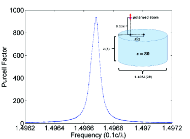
Figure 3: Spontaneous emission enhancement of a polarized atom/molecule placed above a dielectric cylinder that supports a supercavity mode.

IX Conclusion

We have presented a model for lossy, dispersive electromagnetic medium that is valid in the quantum regime. The medium is dispersive because of the coupling of the Maxwellian free fields to a set of Lorentz oscillators. This can be regarded as field-matter coupling in the parlance of previous work [18]. Furthermore, loss is induced in the quantum system by coupling to a collection of simple harmonic oscillators to model noise in a phenomenological manner.

The dispersion comes about because these Lorentz oscillators are sluggish, and their dipole moments cannot be turned on (or off) instantaneously. The coupled system of the Lorentz oscillators to the Maxwellian free field is quantized rigorously here, corresponding to the quantization of a dispersive electromagnetic system. Such quantization is achieved without the need for mode decomposition or diagonalization of the system. Also, such quantization of the coupled system between free fields and matter has not been seen before using this approach. This is advantageous in some systems where finding the normal modes could be a numerically intensive endeavor.

In this work, the coupling of field to matter consists of only one species of Lorentz oscillators. The generalization to the multi-species oscillators case is straightforward and will be shown in our future work.

Also, the loss of the quantum system is obtained by coupling the single oscillator to a bath; the bath induces loss in the single Lorentz oscillator, making its resonance frequency complex. The effect of the noise bath is to shift the resonant frequency of the Lorentz oscillator from being real to a complex number. Meanwhile, the presence of loss requires the appearance of Langevin sources causing the whole system to be energy conserving or quasi-Hermitian in the ensemble average sense. Hence, the loss model is considerably simpler allowing for analytic solution to elucidate the physics behind the loss mechanism. One can also observe the one-way flow of energy from the host quantum system consisting of the Lorentz oscillator to the noise bath. Moreover, the equations of motion are considerably simpler and closer to the classical model. The proximity of the model to classical model allows the ease to incorporate computational electromagnetics methods [62] to solve future quantum problems. The appearance of Langevin sources is commensurate with the physics of the fluctuation dissipation theorem [56, 57, 31, 64, 65]: at thermal equilibrium with a noise bath, energy is lost from the quantum system to the bath, but energy is also returned to the quantum system from the noise bath. A more complicated noise model as expounded in [12] can be assumed. There, more complicated physical processes such as coupling to phonons and electron collisions can give rise to dissipation but this is beyond the scope of this work.

In the previous work involving the coupling between the free-field, matter, and noise bath, the mode decomposition of the entire coupled system is achieved with Fano diagonalization, giving rise to modes which are called polaritons [18]. But here, no diagonalization is necessary, and the resulting quantum equations of motion resemble the classical equations of motion involving Lorentz oscillators. It is hoped that this will enable a simpler model for dissipative quantum electromagnetic systems as well as future quantum technologies.

The ability to model quantum dissipation is important to determine the coherence time of a quantum system. This is especially important in the design of quantum computers where the coherence between qubits (quantum bits) or artificial atoms has to be maintained. This model also points out that in a pure vacuum, there could be no quantum dissipation unless material media are present. As aforementioned, this explains why photons can traverse gigantic distances in our universe.

X Acknowledgement

We are grateful to Dr. Liping YANG of Purdue U for pointing out Louisell’s book to us.

Appendix A Energy Stored in the Field

Neglecting the $1/2$ factor, the Hamiltonian for the vector potential is

$$\mathscr{H}_{A,0}={{\bf\Pi}}_{A}^{2}+\left(\nabla\times{{\bf A}}\right)^{2}+\left(\nabla\cdot{{\bf A}}\right)^{2}={{\bf\Pi}}_{A}^{2}+{{\bf B}}^{2}+\Pi_{\Phi}^{2}$$ (127)

where ${{\bf\Pi}}_{A}=\overset{\bm{.}}{{{\bf A}}}$, $\nabla\cdot{{\bf A}}=-\overset{\bm{.}}{\Phi}$, and ${{\bf B}}=\nabla\times{{\bf A}}$.

$$\mathscr{H}_{\Phi,0}=\Pi_{\Phi}^{2}+\left(\nabla\Phi\right)^{2}$$ (128)

The subscript “0” is used to indicate that these Hamiltonians are the stand-alone Hamiltonians where coupling with the polarization current is not accounted for. Therefore,

$$\mathscr{H}_{A,0}-\mathscr{H}_{\Phi,0}={{\bf\Pi}}_{A}^{2}+{{\bf B}}^{2}-\left(\nabla\Phi\right)^{2}$$ (129)

But

$$\mathscr{H}_{F,0} ={{\bf E}}^{2}+{{\bf B}}^{2}=\left({{\bf\Pi}}_{A}+\nabla\Phi\right)^{2}+{{\bf B}}^{2}$$

$$={{\bf\Pi}}_{A}^{2}+\left(\nabla\Phi\right)^{2}+2\nabla\Phi\cdot{{\bf\Pi}}_{A}+{{\bf B}}^{2}$$ (130)

and

$$2\nabla\Phi\cdot{{\bf\Pi}}_{A} =-2\Phi\nabla\cdot{{\bf\Pi}}_{A}=2\Phi\overset{\bm{..}}{\Phi}=2\Phi(\nabla^{2}\Phi+\varrho)$$

$$=-2\left(\nabla\Phi\right)^{2}+2\varrho\Phi$$ (131)

where integration by parts has been used liberally, since these are integrands embedded in an outer integral, namely, the actual Hamiltonian is related to the Hamiltonian density by an integral. Using the above, then

$$\mathscr{H}_{F,0}={{\bf E}}^{2}+{{\bf B}}^{2}=\mathscr{H}_{A,0}-\mathscr{H}_{\Phi,0}+2\varrho\Phi$$ (132)

The above is important for the derivation of (19).

Appendix B Laplace Transform Approach for Quantum Dissipation

Defining the Laplace transform of $a(t)$ as $A(s)$, one deduce from (68) and (69) that

$$\hat{A}(s)\left(s+i\omega_{0}+\sum_{j}\frac{\gamma_{j}^{2}}{s+i\omega_{j}}\right)=\hat{a}(0)$$ (133)

Assuming that there are infinitely many harmonic oscillators in the bath, then the above summation can be replaced by an integral when the number of modes is infinitely large, and the spacing between their frequencies becomes infinitesimally small. Namely,

$$I(s)=\sum_{j}\frac{\gamma_{j}^{2}}{s+i\omega_{j}} \Rightarrow\frac{1}{2\pi}\int_{-\infty}^{\infty}d\omega\frac{\eta(\omega)}{s+i\omega}$$

$$=\frac{1}{i2\pi}\int_{-\infty}^{\infty}d\omega\frac{\eta(\omega)}{\omega-is}$$ (134)

where $\gamma_{j}^{2}\approx\frac{1}{2\pi}\eta(\omega)\Delta\omega$ and $\omega=\omega_{j}=j\Delta\omega$. A pole is located at $\omega=is$. But the radius of convergence (ROC) on the complex $s$ plane is for $\Re e(s)>0$. Therefore, for $s$ in the ROC, the pole in the complex $\omega$ is above the real $\omega$ axis.

By assuming that $\eta(\omega)\rightarrow 0,\quad|\omega|\rightarrow\infty$ and that $\eta(\omega)$ is analytic, then by invoking Cauchy’s theorem and Jordan’s lemma [63], the above integral can be evaluated in closed form yielding

$$I(s)=\eta(is)$$ (135)

Since $\eta(\omega)$ is real when $\omega$ is real, $\eta(is)$ is approximately real when $is$ is close to the real axis. But, $\eta(s)$ is weakly dependent on $s$, and can be assumed to be independent of frequency $\omega$. Then the pole of the system described by (133) is given by

$$s=-i\omega_{0}-\eta$$ (136)

The above pole corresponds to a dissipative mode representing quantum loss.

If the noise bath oscillators are not set to zero at $t=0$, then the pertinent equation for the initial value problem becomes

$$\hat{A}(s)\left(s+i\omega_{0}+\sum_{j}\frac{\gamma^{2}}{s+i\omega_{j}}\right)=\hat{a}(0)-i\sum_{j}\frac{\gamma_{j}\hat{b}_{j}(0)}{s+i\omega_{j}}$$ (137)

The summation on the left-hand side can again be approximated as before to arrive at

$$\hat{A}(s)\left(s+i\omega_{0}+\eta\right)=\hat{a}(0)-i\sum_{j}\frac{\gamma_{j}\hat{b}_{j}(0)}{s+i\omega_{j}}$$ (138)

It is not possible to find a simple approximation to the summation on the right-hand side since $\hat{b}_{j}(0)$ is a random variable in the noise bath. So it is left unchanged. The above equation can be transformed back to the time domain to yield

$$\overset{\bm{.}}{\hat{a}}=-i\omega_{0}\hat{a}-\eta\hat{a}-i\sum_{j}\gamma_{j}\hat{b}_{j}(0)e^{-i\omega_{j}t}$$ (139)

The above is similar to (75).

Appendix C Proof of Preservation of Commutator

The proof of the preservation of the quantum commutator has been lucidly presented by Tan in [10]. But since it is in Chinese, it is reproduced here. By using the product rule for differentiation, one gets

$$\frac{d}{dt}\left[\hat{a},\hat{a}^{\dagger}\right]=\left[\hat{a},\frac{d}{dt}\hat{a}^{\dagger}\right]+\left[\frac{d}{dt}\hat{a},\hat{a}^{\dagger}\right]$$ (140)

From (77) and (79), one gets

$$\frac{d}{dt}\hat{a}^{\dagger}(t) =i\omega\hat{a}^{\dagger}(t)-\eta\hat{a}^{\dagger}(t)+\hat{F}^{\dagger}(t),$$

$$\frac{d}{dt}\hat{a}(t) =-i\omega\hat{a}(t)-\eta\hat{a}(t)+\hat{F}(t)$$ (141)

From (140)

$$\frac{d}{dt}\left[\hat{a},\hat{a}^{\dagger}\right]=i\omega_{0}\left[\hat{a},\hat{a}^{\dagger}\right]-\eta\left[\hat{a},\hat{a}^{\dagger}\right]+\left[\hat{a},\hat{F}^{\dagger}\right]$$

$$-i\omega_{0}\left[\hat{a},\hat{a}^{\dagger}\right]-\eta\left[\hat{a},\hat{a}^{\dagger}\right]+\left[\hat{F},\hat{a}^{\dagger}\right]$$

$$=-2\eta\left[\hat{a},\hat{a}^{\dagger}\right]+\left[\hat{a},\hat{F}^{\dagger}\right]+\left[\hat{F},\hat{a}^{\dagger}\right]$$ (142)

Integrating the above yields

$$\hat{a}^{\dagger}(t)=\hat{a}^{\dagger}(0)e^{i\omega_{0}t-\eta t}+\int_{0}^{t}d\tau e^{(i\omega_{0}-\eta)(t-\tau)}\hat{F}^{\dagger}(\tau)$$ (143)

$$\hat{a}(t)=\hat{a}(0)e^{-i\omega_{0}t-\eta t}+\int_{0}^{t}d\tau e^{(-i\omega_{0}-\eta)(t-\tau)}\hat{F}(\tau)$$ (144)

The commutators on the right-hand side need to be evaluated, yielding

$$\left[\hat{F}(t),\hat{a}^{\dagger}(t)\right] =\left[\hat{F}(t),\hat{a}^{\dagger}(0)e^{i\omega_{0}t-\eta t}\right]$$

$$+\left[\hat{F}(t),\int_{0}^{t}d\tau\,e^{(i\omega_{0}-\eta)(t-\tau)}\hat{F}^{\dagger}(\tau)\right]$$ (145)

$$\left[\hat{a}(t),\hat{F}^{\dagger}(t)\right] =\left[\hat{a}(0)e^{-i\omega_{0}t-\eta t},\hat{F}^{\dagger}(t)\right]$$

$$+\left[\int_{0}^{t}d\tau e^{(-i\omega_{0}-\eta)(t-\tau)}\hat{F}(\tau),\hat{F}^{\dagger}(t)\right]$$ (146)

Using the definition for the commutator as given in (78), the first term on the right-hand side of the above can be shown to be zero. Then it can be shown that the above becomes

$$\left[\hat{F}(t),\hat{a}^{\dagger}(t)\right]=\int_{0}^{t}d\tau e^{(i\omega_{0}-\eta)(t-\tau)}\left[\hat{F}(t),\hat{F}^{\dagger}(\tau)\right]$$ (147)

It is more prudent to take the ensemble average of the above, as the noise bath can consist of time-varying dipoles, e.g., in Brownian motion. Then

$$\left\langle\left[\hat{F}(t),\hat{a}^{\dagger}(t)\right]\right\rangle=\int_{0}^{t}d\tau e^{(i\omega_{0}-\eta)(t-\tau)}\left\langle\left[\hat{F}(t),\hat{F}^{\dagger}(\tau)\right]\right\rangle$$ (148)

From (V) that

$$\left\langle\left[\hat{F}(t),\hat{F}^{\dagger}(t^{\prime})\right]\right\rangle=\eta\delta(t-t^{\prime})$$ (149)

then

$$\left\langle\left[\hat{F}(t),\hat{a}^{\dagger}(t)\right]\right\rangle=\left\langle\left[\hat{a}(t),\hat{F}^{\dagger}(t)\right]\right\rangle=\eta$$ (150)

Finally, from (C), after taking ensemble average.

$$\frac{d}{dt}\left\langle\left[\hat{a}(t),\hat{a}^{\dagger}(t)\right]\right\rangle=2\eta\left(1-\left\langle\left[\hat{a}(t),\hat{a}^{\dagger}(t)\right]\right\rangle\right)$$ (151)

The above implies that

$$\left\langle\left[\hat{a}(t),\hat{a}^{\dagger}(t)\right]\right\rangle=1$$ (152)

or that the commutator is preserved in the ensemble average sense..

References

- [1]
- [2] J. J. Hopfield, “Theory of the contribution of excitons to the complex dielectric constant of crystals,” Phys. Rev. vol. 112, no. 5, pp. 1555, 1958.
- [3] A. Caldeira and A. J. Leggett, “Influence of dissipation on quantum tunneling in macroscopic systems,” Phys. Rev. Lett., vol. 46, p. 211, 1981.
- [4] C. Cohen-Tannoudji, J. Dupont-Roc, and G. Grynberg, Atom-Photon Interactions: Basic Processes and Applications. John Wiley & Sons, New York, NY, 1992.
- [5] L. Mandel, and E. Wolf, Optical Coherence and Quantum Optics. Cambridge University Press, Cambridge, UK, 1995.
- [6] M. O. Scully, and M. S. Zubairy, Quantum Optics. Cambridge University Press, Cambridge, UK, 1997.
- [7] H. A. Haus, Electromagnetic Noise and Quantum Optical Measurements. Springer-Verlag, Berlin, Heidelberg, 2000.
- [8] R. Loudon, The Quantum Theory of Light. Oxford University Press, Oxford, UK, 2000.
- [9] W. Vogel and D-G. Welsch, Quantum Optics. Wiley-VCH, Berlin, Heidelbreg, 2006.
- [10] W. H. Tan, Introduction to Quantum Optics. Science Press, China, 2008 (in Chinese).
- [11] J. Garrison, and J. Chiao, Quantum Optics. Oxford University Press, Oxford, UK, 2014.
- [12] M. Kira and S. W. Koch, Semiconductor Quantum Optics. Cambridge University Press, Cambridge, UK, 2011.
- [13] C. Gerry, and P. Knight, Introductory Quantum Optics. Cambridge University Press, Cambridge, UK, 2005.
- [14] M. Fox, Quantum Optics: An Introduction. Oxford University Press, Oxford, UK, 2006.
- [15] D. F. Walls and G. J. Milburn, Quantum Optics. Springer Science & Business Media, Berlin, Heidelberg, 2007.
- [16] R. Loudon. “The propagation of electromagnetic energy through an absorbing dielectric,” J. Phys. A, vol. 3, no. 3, pp. 233, 1970.
- [17] R. J. Glauber and M. Lewenstein, “Quantum optics of dielectric media,” Phys. Rev. A, vol. 43, pp. 467, 1991.
- [18] B. Huttner and S. M. Barnett. “Quantization of the electromagnetic field in dielectrics,” Phys. Rev. A, vol. 46, no. 7, pp. 4306, 1992.
- [19] P. W. Milonni, “Field quantization and radiative processes in dispersive dielectric media,” J. Mod. Opt., vol. 42, no. 10, pp. 1991-2004, 1995.
- [20] T. Grunner and D.-G. Welsch. “Green-function approach to the radiation-field quantization for homogeneous and inhomogeneous Kramers-Kronig dielectrics,” Phys. Rev. A, vol. 53, no. 3, pp. 1818, 1996.
- [21] H. T. Dung, L. Knoll, D.-G. Welsch. “Three-dimensional quantization of the electromagnetic field in dispersive and absorbing inhomogeneous dielectrics,” Phys. Rev. A, vol. 57, no. 5, pp. 3931, 1998.
- [22] R. Ruppin, “Electromagnetic energy density in a dispersive and absorptive material,” Phys. Lett. A, vol. 299, no. 2, pp. 309-312, 2002.
- [23] H. T. Dung, S. Y. Buhmann, L. Knöll, D.-G. Welsch, S. Scheel, and J. Kästel, “Electromagnetic-field quantization and spontaneous decay in left-handed media,” Phys. Rev. A, vol. 68, no. 4, pp. 043816, 2003.
- [24] S. Scheel and S. Y. Buhmann, “Macroscopic quantum electrodynamics-concepts and applications,” Acta Physica Slovaca, vol. 58, no. 5, pp. 675, 2008.
- [25] L. G. Suttorp and M. Wubs, “Field quantization in inhomogeneous absorptive dielectrics,” Phys. Rev. A, vol. 70, no. 1, pp. 013816, 2004.
- [26] L. G. Suttorp, “Field quantization in inhomogeneous anisotropic dielectrics with spatio-temporal dispersion,” J. Phys. A: Math. Theo., vol. 40, no. 13, pp. 3697, 2007.
- [27] T. G. Philbin, “Canonical quantization of macroscopic electromagnetism,” New J. Phys., vol. 12, pp. 123008, 2010.
- [28] R.-C. Ge, J.F. Young, and S. Hughes, “Quasi-normal mode approach to the local-field problem in quantum optics,” Optica, vol. 2, no. 3, pp. 246-249, 2015.
- [29] M. K. Dezfouli and S. Hughes, “Quantum optics model of surface enhanced raman spectroscopy for arbitrarily shaped plasmonic resonators,” ACS Photonics, vol. 4, no. 5, pp. 1245-1256, 2017.
- [30] Z. H. Peng, S. E. de Graaf, J. S. Tsai and O. V. Astafiev, “Tuneable on-demand single-photon source in the microwave range,” Nat. Comm., vol. 7, pp. 12588, 2016.
- [31] H. B. Callen and T. A. Welton, “Irreversibility and generalized noise,” Phys. Rev., vol. 83, pp. 34-40, 1951.
- [32] R. Kubo, “The fluctuation-dissipation theorem,” Rep. Prog. Phys., vol. 29, pp. 255, 1966.
- [33] G. S. Agarwal, “Quantum electrodynamics in the presence of dielectrics and conductors. I. Electromagnetic-field response functions and black body fluctuation in finite geometries,” Phys. Rev. A, vol. 11, no. 1, pp. 230-242, 1975.
- [34] G. S. Agarwal, “Quantum electrodynamics in the presence of dielectrics and conductors. III. Relations among one-photon transition probabilities in stationary and nonstationary fields, density of states, the field-correlation functions, and surface-dependent response functions,” Phys. Rev. A, vol. 11, no. 1, pp. 253-264, 1975.
- [35] P. Langevin, “Sur la théorie du mouvement brownien [On the Theory of Brownian Motion],” C. R. Acad. Sci. (Paris), vol. 146, pp. 530-533, 1908.
- [36] U. Fano, “Effects of configuration interaction on intensities and phase shifts,” Phys. Rev., vol. 124, no. 6, pp. 1866-1878, 1961.
- [37] R. Kronig and H. A. Kramers, ”Absorption and dispersion in x-ray spectra,” Z. Phys, vol. 48, no. 174, 1928.
- [38] L. V. Keldysh, “Diagram technique for nonequilibrium processes,” Sov. Phys. JETP, vol. 20, no. 4, pp. 1018-1026, 1965.
- [39] S. Datta, Quantum Transport: Atom to Transistor. Cambridge University Press, 2005.
- [40] W. C. Chew, A. Y. Liu, C. Salazar-Lazaro, and W. E. I. Sha, “Quantum Electromagnetics: A New Look, Part I,” IEEE J. Multiscale and Multiphysics Comp. Tech., vol. 1, pp. 73-84, 2016.
- [41] W. C. Chew, A. Y. Liu, C. Salazar-Lazaro, and W. E. I. Sha, “Quantum Electromagnetics: A New Look, Part II,” IEEE J. Multiscale and Multiphysics Comp. Tech., vol. 1, pp. 85-97, 2016.
- [42] In order to present in this paper a formulation of dissipative quantum electromagnetic systems with the least amount of concepts foreign to the classical electromagneticist, we have elected not to adopt the standard Coulomb gauge treatment and avoid using the Lagrangian formulation. In the Coulomb gauge, all redundancies in the electromagnetic system is removed. Hence, quantization can be done without any special treatment of the absent longitudinal vector potential and scalar potential (non-Coulomb potential part). Admittedly, in the Lorenz gauge used in this paper, one has to employ some post processing to correctly interpret the quantized and . However, the transverse and longitudinal dynamics in the field-matter system considered here completely decouples. It can be shown that and evolves independent of the other dynamical variables. This is true for this system both classically and quantum mechanically. As such, the difference between using the Coulomb and Lorenz gauge is only formal. We will demonstrate the details of the decoupling as well as the necessary post processing in a future publication. The standard treatment can be found in classical texts such as [4, 6, 11, 20], and have been applied to the dissipative electromagnetic system in the literature [18, 27].
- [43] W. H. Louisell, Quantum Statistical Properties of Radiation. John Wiley & Sons, Hoboken, NJ, 1973.
- [44] W. D. Oliver and P. B. Welander, “Materials in superconducting quantum bits,” MRS Bulletin, vol. 38, pp. 816-825, 2013.
- [45] T. Lancaster and S. J. Blundell, Quantum Field Theory for the Gifted Amateur. Oxford University Press, Oxford, UK, 2014.
- [46] It is to be noted that the coupling to the Drude-Lorentz-Sommerfeld oscillator to obtain a classical dispersion model for the medium has also been used in [48].
- [47] In this unit, the velocity of light is one, and it can be achieved by either redefining the unit for time or length such that the velocity of light is one unit length per unit time. Also, the units for , , and can be redefined such that energy density is proportional to , , and . Here, the unit for length is redefined so that one unit length is m for one second. Alternatively, one can take one unit length to be m for one nano-second.
- [48] A. Raman and S. Fan, “Photonic band structure of dispersive metamaterials formulated as a Hermitian eigenvalue problem,” Phys. Rev. Lett., vol. 104, no. 8, pp. 087401, 2010.
- [49] W. C. Chew, “Vector potential electromagnetics with generalized gauge for inhomogeneous media: formulation,” PIER, vol. 149, pp. 69-84, 2014.
- [50] The raison d’etre for this will be given in our future work.
- [51] This equation is found in standard quantum theory text, and also explained in [40].
- [52] Notice the sign difference for the canonical commutator of the scalar potential. This sign reversal is needed due to the negative contribution of the scalar potential in the Hamiltonian.
- [53] The bath oscillators are mathematically similar to the Lorentz oscillator.
- [54] H. Goldstein, Classical Mechanics. Pearson Education, India, 1965.
- [55] M. Lax, “Quantum noise. IV. quantum theory of noise sources,” Phys. Rev., vol 145, pp. 110, 1966.
- [56] J. B. Johnson, “Thermal agitation of electricity in conductors,” Phys. Rev., vol. 32, pp. 97, 1928.
- [57] H. Nyquist, “Thermal agitation of electric charge in conductors,” Phys. Rev., vol. 32, pp. 110, 1928.
- [58] L. Novotny and B. Hecht, Principles of Nano-Optics. Cambridge University Press, New York, 2006.
- [59] P. F. Qiao, W. E. I. Sha, W. C. H. Choy, and W. C. Chew, “Systematic study of spontaneous emission in a two-dimensional arbitrary inhomogeneous environment,” Phys. Rev. A, vol. 83, no. 4, pp. 043824, Feb. 2011.
- [60] Y. P. Chen, W. E. I. Sha, W. C. H. Choy, L. J. Jiang, and W. C. Chew, “Study on spontaneous emission in complex multilayered plasmonic system via surface integral equation approach with layered medium Green’s function,” Opt. Express, vol. 20, no. 18, pp. 20210-20221, Aug. 2012.
- [61] M. V. Rybin, K. L. Koshelev, Z. F. Sadrieva, K. B. Samusev, A. A. Bogdanov, M. F. Limonov, and Y. S. Kivshar, “High-Q supercavity modes in subwavelength dielectric resonators,” Phys. Rev. Lett, vol. 119, pp. 243901, Dec. 2017.
- [62] W. C. Chew, J. M. Jin, E. Michielssen, and J. M. Song (editors.), Fast and Efficient Algorithms in Computational Electromagnetics. Artech House, Norwood, MA, 2001.
- [63] F. B. Hildebrand, Advanced Calculus for Applications. vol. 63, Prentice-Hall, Englewood Cliffs, NJ, 1962.
- [64] P. W. Milonni, The Quantum Vacuum: An Introduction to Quantum Electrodynamics. Academic Press, San Diego, CA, 1994.
- [65] S. Rytov, Y. Kravtsov, V. Tatarskii, Principles of Statistical Radiophysics. vol. 3, Springer-Verlag, Berlin, Heidelberg, 1989.