Approximation Algorithms for Barrier Sweep Coverage

Abstract

Time-varying coverage, namely sweep coverage is a recent development in the area of wireless sensor networks, where a small number of mobile sensors sweep or monitor comparatively large number of locations periodically. In this article we study barrier sweep coverage with mobile sensors where the barrier is considered as a finite length continuous curve on a plane. The coverage at every point on the curve is time-variant. We propose an optimal solution for sweep coverage of a finite length continuous curve. Usually energy source of a mobile sensor is battery with limited power, so energy restricted sweep coverage is a challenging problem for long running applications. We propose an energy restricted sweep coverage problem where every mobile sensors must visit an energy source frequently to recharge or replace its battery. We propose a $\frac{13}{3}$-approximation algorithm for this problem. The proposed algorithm for multiple curves achieves the best possible approximation factor 2 for a special case. We propose a 5-approximation algorithm for the general problem. As an application of the barrier sweep coverage problem for a set of line segments, we formulate a data gathering problem. In this problem a set of mobile sensors is arbitrarily monitoring the line segments one for each. A set of data mules periodically collects the monitoring data from the set of mobile sensors. We prove that finding the minimum number of data mules to collect data periodically from every mobile sensor is NP-hard and propose a 3-approximation algorithm to solve it.

Key words: Barrier coverage, Sweep Coverage, Approximation Algorithm, Eulerian Graph, TSP, Mobile Sensor, Data Mule, Data Gathering, Wireless Sensor Networks.

1 Introduction

Coverage is a widely studied research area and one of the most important problem in wireless sensor networks (WSNs) for monitoring, surveillance, etc. Based on the subject to be covered by a set of sensors, it is classified into three categories, such as point coverage, area coverage and barrier coverage. In point coverage [14, 21], a set of points are covered, whereas in area coverage [3, 24, 28], all points inside a bounded area are covered. But in barrier coverage, barriers of sensors are required for an appropriate model of coverage for applications like detecting intruders when they cross borders or detecting spread of pollutants, chemicals when sensors are deployed around critical regions. In most of barrier coverage literatures [5, 16, 20, 23, 30] static sensors are usually used for continuous monitoring the borders or boundaries. But there are applications [9], where time-variant coverage at every point on a boundary is sufficient instead of monitoring all along. For these kind of applications, deployment of static sensors at the boundary is not cost effective in terms of resource utilization for periodic monitoring every point on the boundary. The time-variant coverage can be solved efficiently by utilizing less number of resources i.e., mobile sensors with appropriate movement strategy. The cost involvement aspect of this solution is mobility and storage capacity of the mobile sensors. This type of coverage problems, where time-variant coverage is sufficient for periodic petrol inspections are termed as sweep coverage. In point sweep coverage problem [7, 9, 11, 19, 29], a given set of discrete points are monitored by a set of mobile sensors at least once within a given period of time. This time period is termed as sweep period. The primary motivation of these sweep coverage problems is to utilize minimum number of mobile sensors for achieving the goal. But finding minimum number of mobile sensors for the sweep coverage of a given set of discrete points on a plane is NP-hard [19]. The area sweep coverage problem is introduced in the article [11], where it is proved that the problem is NP-complete. In this article, we formulate different variation of barrier sweep coverage problems for covering finite length curves on a plane.

1.1 Contribution

In this paper, our contributions on sweep coverage problems are as follows:

• We introduce barrier sweep coverage problems for covering finite length curves on a plane. We solve the problem optimally with minimum number of mobile sensors for a finite length curve.

• We define an energy restricted barrier sweep coverage problem and propose a $\frac{13}{3}$-approximation algorithm for a finite length curve.

• A $2$-approximation algorithm is proposed for solving the sweep coverage problem for multiple curves for a special case where each mobile sensor visits all points of each curve. For the general version of the problem, a 5-approximation algorithm is proposed.

• We formulate a data gathering problem by a set of data mules and a $3$-approximation algorithm is proposed to solve the NP-hard problem.

• Performance of the proposed algorithms are investigated through simulation for multiple finite length curves.

1.2 Related Work

The concept of sweep coverage initially came from the context of robotics [2]. In [2], the authors considered a dynamic sensor coverage problem using mobile robots in absence of global localization information. The sensors are mobilized by mounting them on the mobile robots. The robots explore an unexplored area by deploying small communication beacons. The robots decide direction of movements during the exploration using local markers with the beacons. Recently, several works [7, 9, 19, 26, 27, 29, 31] on sweep coverage are proposed in WSNs. Most of the works focused on designing suitable heuristics. In [29], the authors considered a network consisting static and mobile sensors. Two different problems are considered in that paper. In the first problem, objective is to minimize number of mobile sensors that can guarantee data download from every static sensor in a given time period with high probability. In the second problem, objective is to guide mobile sensors for moving towards static sensors without any centralized control. In the first heuristic (MinExpand), mobile sensors move in the same path in every time period. In the second heuristic (OSweep), the mobile sensors move in different paths in different time periods. Hung et al. [7] considered a sweep coverage problem where nonuniform deployment of a set of PoIs is made over an area of interest. The area is divided into smaller sub-areas. Then mobile sensors are deployed over the sub-areas, one for each, to guarantee sweep coverage of all the PoIs in the respective sub-areas. Due to unequal number of PoIs in different sub-areas, sweep periods (patrolling times) of the mobile sensors may not be same. Objective of the proposed heuristic is to make the patrolling time approximately same for all mobile sensors. In [26], the authors considered a problem where sweep periods of the PoIs are different. A scheme is proposed based on periodic vehicle routing problem to minimize number of unnecessary visits of a PoI by a mobile sensor. To extend lifetime of sweep coverage, Yang et al. [31] utilized base station as a power source for periodical refueling or replacing battery of the mobile sensors. The authors proposed two heuristics with one base station and multiple base stations, respectively. Hardnass of the sweep coverage problem is studied by Li et al. [19] theoretically. The authors proved that finding minimum number of mobile sensors to sweep cover a set of PoIs is NP-hard. It is proved that the problem cannot be approximated less than a factor of 2, unless P=NP. A $(2+\epsilon)$-approximation and a 3-approximation algorithms are proposed to solve the problem. The authors remarked on impossibility of design distributed local algorithm to guarantee sweep coverage of all PoIs, i.e., a mobile sensor cannot locally determine whether all PoIs are sweep covered without global information. But there is a flaw in the approximation algorithms. We, in [12], remarked on the flaw of the 3-approximation algorithm [19] and proposed corrected algorithm keeping same approximation factor to guarantee sweep coverage for the given set of PoIs. If the sweep periods of the PoIs are different, a $O(\log\rho)$-approximation algorithm we proposed where $\rho$ is the ratio of the maximum and minimum sweep periods. An inapproximability result is also established when the speed of the mobile sensors are not necessarily same. In [11], a 2-approximation algorithm for a special case of point sweep coverage problem we proposed, which is the best possible approximation factor according to the result in [19]. A distributed 2-approximation algorithm we proposed for the point sweep coverage problem, where static sensors are deployed at the PoIs and those are considered as PoIs. The static sensors communicate among them self through message to find initial deployment locations of the mobile sensors. The area sweep coverage problem is formulated and proved that the problem is NP-complete. A $2\sqrt{2}$ approximation algorithm is proposed to solve the problem for a square region. The area sweep coverage problem for arbitrary bounded region is also investigated in that paper. An energy efficient sweep coverage problem is proposed in [13], where a set of static and mobile sensors are used for sweep coverage of a set of discrete points. The objective is to minimize the total energy consumption per unit time by the set of sensors guaranteeing the required sweep coverage. An 8-approximation algorithm is proposed to solve the problem.

There are similar patrolling problems [8, 10, 15] like sweep coverage with different objectives. Objective of the problems is to minimize time between two consecutive visits of any point while monitoring a given road network or boundary of a region by a set of mobile agents having different speeds. In [8], the authors proposed two strategies; partition based strategy and cycle based strategy to obtain movement schedules of the mobile agents. The authors proved that the strategy obtains optimal solution when number of agents is less than or equal to 2 for partition strategy and number of agents is less than or equal to 4 for cycle strategy. Kawamura et al. [15] proved that the partition strategy proposed in the paper [8] achieves optimal solution for number of agents less than or equal to 3.

The rest of the paper is organized as follows. The problem definitions are given in section 2. Barrier sweep coverage for single curve and multiple curves are discussed in section 3 and section 4 respectively. A data gathering problem by data mules is formulated and discussed in section 5. Finally, conclude and future works are given in section 7.

2 Problem Definitions

Let ${\mathcal{C}}$ be a finite length curve on a 2D plane. ${\mathcal{C}}$ is said to be covered by a set of sensors if and only if each point on ${\mathcal{C}}$ is covered by at least one sensor. Based on the above coverage metric, the definitions of barrier sweep coverage problems are given below.

Definition 1

($t-$barrier sweep coverage) Let ${\mathcal{C}}$ be any finite length curve on a 2D plane and ${\mathcal{S}}=\{s_{1},s_{2},\cdots,s_{m}\}$ be a set of mobile sensors. ${\mathcal{C}}$ is said to be $t$-barrier sweep covered if and only if each point of ${\mathcal{C}}$ is visited by at least one mobile sensor in every time period $t$.

Definition 2

(Barrier sweep coverage problem for single finite length curve) Let ${\mathcal{C}}$ be a finite length curve and ${\mathcal{S}}=\{s_{1},s_{2},\cdots,s_{m}\}$ be a set of mobile sensors. For given $t>0$ and $v>0$, find the minimum number of mobile sensors with uniform speed $v$ such that all points of ${\mathcal{C}}$ are visited by all mobile sensors and ${\mathcal{C}}$ is $t$-barrier sweep covered.

Definition 3

(Barrier sweep coverage problem for multiple finite length curves (BSCMC)) Let ${\mathcal{X}}=\{{\mathcal{C}}_{1},{\mathcal{C}}_{2},\cdots,{\mathcal{C}}_{n}\}$ be a set of $n$ finite length curves and ${\mathcal{S}}=\{s_{1},s_{2},\cdots,s_{m}\}$ be a set of mobile sensors. For given $t>0$ and $v>0$, find the minimum number of mobile sensors with uniform speed $v$ such that each ${\mathcal{C}}_{i}$ for $i=1,2,\cdots,n$ is $t$-barrier sweep covered.

In general sensors are equipped with limited battery power. In order to continue sweep coverage for long time, each mobile sensor must visits an energy source to recharge or replace its battery. Let $T$ be the maximum travel time for a mobile sensor starting with full powered battery maintaining uniform speed $v$ till battery power goes off. Let $e$ be an energy source on the plane and every mobile sensor can recharge or replace its battery by visiting $e$. We define energy restricted barrier sweep coverage problem for a finite length curve ${\mathcal{C}}$ as given below.

Definition 4

(Energy restricted barrier sweep coverage problem) Given a finite length curve ${\mathcal{C}}$, an energy source $e$ and $v,t,T>0$, find the minimum number of mobile sensors with the uniform speed $v$ such that each point of ${\mathcal{C}}$ can be visited by at least one mobile sensor in every $t$ time period and each mobile sensor visits $e$ once in every $T$ time period.

3 Barrier sweep coverage for a finite length curve

In this section, first we propose a solution for finding the optimal number of mobile sensors to sweep cover a finite length curve. Later, we give an approximate solution for the energy restricted barrier sweep coverage problem for a finite length curve.

3.1 Optimal solution for a finite length curve

The barrier sweep coverage problem for a finite length curve can be optimally solved using the following strategy. Let $|{\mathcal{C}}|$ be the length of the curve ${\mathcal{C}}$. If ${\mathcal{C}}$ is a closed curve, then partition ${\mathcal{C}}$ into $\left\lceil\frac{|{\mathcal{C}}|}{vt}\right\rceil$ equal parts of length $vt$ and deploy total $\left\lceil\frac{|{\mathcal{C}}|}{vt}\right\rceil$ mobile sensors, one at each of the partitioning points. Then each mobile sensor starts moving at same time along ${\mathcal{C}}$ in the same direction to ensure $t$-sweep coverage of ${\mathcal{C}}$. If ${\mathcal{C}}$ is an open curve, then join the end points of ${\mathcal{C}}$ to make it close and apply the same strategy as above.

3.2 Energy restricted barrier sweep coverage for a finite length curve

In this section we propose an approximate solution for the energy restricted barrier sweep coverage problem. The approximation factor of the proposed algorithm is $\frac{13}{3}$ though it is not known whether the problem is NP-hard or not. Let $e$ be the energy source on the plane. To make the problem feasible, we assume that the distance of any point on ${\mathcal{C}}$ from $e$ is less than $\frac{vT}{2}$. We define a tour named as $e$-tour which is denoted as $\{e,p,q,e\}$, that starts from $e$, visits $arc(pq)$ of ${\mathcal{C}}$ continuously and then ends at $e$ such that total length of the tour is at most $vT$, where $p$ and $q$ are two points on ${\mathcal{C}}$. The objective of our technique is to find a tour through $e$ and ${\mathcal{C}}$, which is concatenation of multiple number of $e$-tours. Let $d(a,b)$ the Euclidean distance between two points $a$ and $b$ and $d_{c}(p,q)$ be the distance between two points $p$ and $q$ along ${\mathcal{C}}$ in the clockwise direction, where $p$ and $q$ are two points on ${\mathcal{C}}$. So, $d_{c}(p,q)$ is equal to the length of the $arc(pq)$.

\psfrag{x}{$i_{1}$}\psfrag{y}{$i_{2}$}\psfrag{z}{$i_{3}$}\psfrag{w}{$i_{4}$}\psfrag{e}{$e$}\includegraphics[width=173.44534pt]{e-tour.eps}

Figure 1: Showing selection of $e$-tours $\{e,i_{1},i_{2},e\}$, $\{e,i_{2},i_{3},e\}$, $\{e,i_{3},i_{4},e\},\cdots$

Let us chose any point $i_{1}$ on a finite length ‘closed’ curve ${\mathcal{C}}$. Find a point $i_{2}$ on ${\mathcal{C}}$ in the clockwise direction of ${\mathcal{C}}$ (Ref. Fig. 1) such that $d_{c}(i_{1},i_{2})=\frac{vT}{2}-d(e,i_{1})$. Here $T_{1}=\{e,i_{1},i_{2},e\}$ is a $e$-tour, since length of $T_{1}$ is equal to $d(e,i_{1})+d_{c}(i_{1},i_{2})+d(i_{2},e)\leq d(e,i_{1})+\frac{vT}{2}-d(e,i_{1})+\frac{vT}{2}$ = $vT$, as shown in Fig. 1. Next $e$-tour is selected as $\{e,i_{2},i_{3},e\}$, where $i_{3}$ is a point on ${\mathcal{C}}$ in the clockwise direction from $i_{2}$ such that $d_{c}(i_{1},i_{2})=\frac{vT}{2}-d(e,i_{2})$. Once the second tour is selected, we check whether the combination of the previous tour and current tour together, i.e., $\{e,i_{1},i_{3},e\}$ form an $e$-tour or not. If the combined tour $\{e,i_{1},i_{3},e\}$ is a valid $e$-tour, then the previous tour $\{e,i_{1},i_{2},e\}$ is updated into $\{e,i_{1},i_{3},e\}$ and proceed to select next $e$-tour. This updating of the previous $e$-tour with current one will continue until combined tour violates the length constraint of $e$-tour i.e., length of the combined tour is greater than $vT$. In general, after computing an $e$-tour $T_{j}=\{e,i_{j},i_{j+1},e\}$, we select next point $i_{j+2}$ on ${\mathcal{C}}$ such that $d_{c}(i_{j+1},i_{j+2})=\frac{vT}{2}-d(e,i_{j+1})$. Then if $\{e,i_{j},i_{j+2},e\}$ this is a valid $e$-tour, we update the tour $T_{j}$ as $T_{j}=\{e,i_{j},i_{j+2},e\}$. Otherwise the tour $T_{j+1}$ is selected as $T_{j+1}=\{e,i_{j+1},i_{j+2},e\}$. Continuing this way we decompose ${\mathcal{C}}$ into multiple number of $e$-tours such that every point on ${\mathcal{C}}$ is included in some $e$-tour. If ${\mathcal{C}}$ is an ‘open’ curve, we use the above technique to decompose ${\mathcal{C}}$ into multiple number of $e$-tours considering one end point of ${\mathcal{C}}$ as $i_{1}$ and continue till the other end point of it. Note that according to the above construction of the $e$-tour, length of the combined tour of two consecutive $e$-tours is always greater than $vT$.

Let $APPRX$ be the total tour after concatenation of the $e$-tours, $T_{1},T_{2},T_{3},\cdots$ one after another in order of obtained by the above technique. For example $T_{1}=\{e,i_{1},i_{2},e\}$, $T_{2}=\{e,i_{2},i_{3},e\}$, $T_{3}=\{e,i_{3},i_{4},e\},\cdots$ are $e$-tours as shown in Fig. 1, where concatenation of those tours is $T_{1}\cdot T_{2}\cdot T_{3}\cdot\cdots$ =$\{e,i_{1},i_{2},e\}\cdot\{e,i_{2},i_{3},e\}\cdot\{e,i_{3},i_{4},e\}\cdot\cdots$ = $\{e,i_{1},i_{2},e,i_{2},i_{3},e,i_{3},i_{4},e,\cdots\}$, where ‘$\cdot$’ is denoted as the concatenation operation of the $e$-tours. Let $|APPRX|$ be the length of $APPRX$. Divide $APPRX$ into equal parts of length $vt$ and deploy one mobile sensor at each of the partitioning points. The mobile sensors then start moving along $APPRX$ in the same direction to ensure sweep coverage of ${\mathcal{C}}$ for desirable long-time. The Algorithm 1(EnergyRestrictedBSC) given below for energy restricted barrier sweep coverage is applicable for closed curve. Though same Algorithm is also applicable for an open curve as explained in the previous paragraph.

Algorithm 1 EnergyRestrictedBSC

1:  Choose any point $i_{1}$ on ${\mathcal{C}}$.

2:  ${\mathcal{C}}^{\prime}={\mathcal{C}}$, $n^{\prime}=1$.

3:  while ${\mathcal{C}}^{\prime}\neq\phi$ do

4:     if $d(e,i_{n^{\prime}})+|{\mathcal{C}}^{\prime}|\leq\frac{vT}{2}$ then

5:        $h=i_{1}$

6:     else

7:        Select a point $h$ on ${\mathcal{C}}$ in a clockwise direction from $i_{n^{\prime}}$ such that $d(i_{n^{\prime}},h)=\frac{vT}{2}-d(e,i_{n^{\prime}})$

8:     end if

9:     if $n^{\prime}\neq 1$ and $d(e,i_{{n^{\prime}}-1})+d_{c}(i_{{n^{\prime}}-1},h)+d(e,h)\leq vT$ then

10:        ${\mathcal{C}}^{\prime}={\mathcal{C}}^{\prime}\setminus arc(i_{n^{\prime}}h)$

11:        $i_{n^{\prime}}=h$, $T_{{n^{\prime}}-1}=\{e,i_{{n^{\prime}}-1},i_{n^{\prime}},e\}$

12:     else

13:         $i_{{n^{\prime}}+1}=h$, $T_{n^{\prime}}$ = $\{e,i_{n^{\prime}},i_{{n^{\prime}}+1},e\}$

14:        ${\mathcal{C}}^{\prime}={\mathcal{C}}^{\prime}\setminus arc(i_{n^{\prime}}i_{{n^{\prime}}+1})$

15:        $n^{\prime}=n^{\prime}+1$

16:     end if

17:     ${\mathcal{C}}^{\prime}={\mathcal{C}}^{\prime}\setminus arc(i_{n^{\prime}}i_{{n^{\prime}}+1})$

18:  end while

19:  $APPRX=T_{1}\cdot T_{2}\cdot T_{2}\cdot\cdots\cdot T_{n^{\prime}}$, where ‘$\cdot$’ is denoted as concatenation operation.

20:  Divide $APPRX$ into equal parts of length $vt$ and deploy one mobile sensor at each of the partitioning points.

21:  All mobile sensor start moving along $APPRX$ at same time in same direction.

Theorem 3.1

According to the Algorithm 1, each mobile sensor visits $e$ in every $T$ time period and each point on ${\mathcal{C}}$ is visited by at least one mobile sensor in every $t$ time period.

Proof

According to our proposed Algorithm 1, the mobile sensors move along the tour $APPRX$. As the length of each $e$-tour is less than or equals to $vT$, the mobile sensors will visit $e$ after traveling at most $vT$ distance since its last visit of $e$. Therefore, each mobile sensor visits $e$ once in every $T$ time period. Again, the mobile sensors are deployed at every partitioning points of $APPRX$ and two consecutive partitioning points are $vt$ distance apart. The relative distance between any two consecutive mobile sensors is $vt$ at any time as they are moving in same speed $v$ along the same direction. Therefore, any point on ${\mathcal{C}}$, which is visited at time $t_{0}$ (say) by a mobile sensor visits again within time $t+t_{0}$ by the next mobile sensor following it. ∎

To analyze the approximation factor with respect to the optimal solution, we consider some special points on ${\mathcal{C}}$ as follows. Let $i_{p}^{1}$, $i_{p}^{2}$ be two special points on the $arc(i_{p}i_{p+1})$ of ${\mathcal{C}}$ such that the $arc(i_{p}i_{p+1})$ is partitioned into three equal parts, i.e., the length of $arc(i_{p}i_{p}^{1})$ equal to the length of $arc(i_{p}^{1}i_{p}^{2})$ equal to the length of $arc(i_{p}^{2}i_{p+1})$. We define a set of points, ${\mathcal{I}}=\{i_{j},i_{j}^{1},i_{j}^{2}|j=1~{}\text{to}~{}n^{\prime}\}$. Following two Lemmas give an upper bound of the length of the tour $APPRX$ and a lower bound of the length of the optimal tour respectively.

Lemma 1

$$|APPRX|\leq\frac{1}{3}\left(2\sum_{j}\left(d(e,i_{j})+d(e,i_{j}^{1})\\ +d(e,i_{j}^{2})\right)+5|{\mathcal{C}}|\right)$$

.

Proof

According to the Algorithm 1, total length of the tour $APPRX$ is

$$|APPRX| = d(e,i_{1})+d_{c}(i_{1},i_{2})+d(i_{2},e)+d(e,i_{2})$$ (1)

$$+d_{c}(i_{2},i_{3})+d(i_{3},e)+\cdots+d(e,i_{1})$$

$$= |{\mathcal{C}}|+2\sum_{j}d(e,i_{j}).$$

Now by triangle inequality,

$$d(e,i_{j}) \leq d(e,i_{j}^{1})+d_{c}(i_{j},i_{j}^{1})~{}{\rm and}$$

$$d(e,i_{j}) \leq d(e,i_{j}^{2})+d_{c}(i_{j},i_{j}^{2})$$

Therefore,

$$|APPRX| \leq |{\mathcal{C}}|+2\sum_{j}\left(d(e,i_{j}^{1})+d_{c}(i_{j},i_{j}^{1})\right)$$ (2)

$$|APPRX| \leq |{\mathcal{C}}|+2\sum_{j}\left(d(e,i_{j}^{2})+d_{c}(i_{j},i_{j}^{2})\right)$$ (3)

From above the equation 1, 2 and 3, we can write,

$$3|APPRX| \leq 3|{\mathcal{C}}|+2\sum_{j}d(e,i_{j})+2\sum_{j}\left(d(e,i_{j}^{1})+d_{c}(i_{j},i_{j}^{1})\right)$$ (4)

$$+2\sum_{j}\left(d(e,i_{j}^{2})+d_{c}(i_{j},i_{j}^{2})\right)$$

As the points $i_{j}^{1}$ and $i_{j}^{2}$ divide length of the $arc(i_{j}i_{j+1})$ into three equal parts, therefore,
$\displaystyle\sum_{j}d_{c}(i_{j},i_{j}^{1})=\frac{|{\mathcal{C}}|}{3}$ and $\displaystyle\sum_{j}d_{c}(i_{j},i_{j}^{2})=\frac{2|{\mathcal{C}}|}{3}$. Using these two results, equation 4 can be written as:

$$3|APPRX| \leq 3|{\mathcal{C}}|+2\sum_{j}\left(d(e,i_{j})+d(e,i_{j}^{1})+d(e,i_{j}^{2})\right)+2\frac{|{\mathcal{C}}|}{3}+2\frac{2|{\mathcal{C}}|}{3}$$

$$|APPRX| \leq \frac{1}{3}\left(2\sum_{j}\left(d(e,i_{j})+d(e,i_{j}^{1})+d(e,i_{j}^{2})\right)\right)+\frac{5}{3}|{\mathcal{C}}|.$$

∎

\psfrag{x}{$p$}\psfrag{y}{$i_{j}$}\psfrag{z}{$i_{j+1}$}\psfrag{w}{$i_{j-1}$}\psfrag{p}{$q$}\psfrag{q}{$i_{j+2}$}\psfrag{e}{\vspace{1cm}$e$}\includegraphics[width=173.44534pt]{opt_tour.eps}

Figure 2: Showing one $e$-tour $OPT_{l}=\{e,p,q,e\}$ of the optimal tour $OPT$

Lemma 2

Let $OPT$ be the optimal tour of the mobile sensors and $|OPT|$ be length of $OPT$, then

$$|OPT|\geq\max\left\{\frac{1}{4}\sum_{j}\left(d(e,i_{j})+d(e,i_{j}^{1})+d(e,i_{j}^{2})\right),|{\mathcal{C}}|\right\}$$

.

Proof

Let $OPT_{l}=\{e,p,q,e\}$ be an $e$-tour of the optimal tour $OPT$ (Ref. Fig. 2). We claim that at most one $arc(i_{j}i_{j+1})$, part of an $e$-tour computed using the Algorithm 1 for some $j$, can be completely contained in $arc(pq)$, where $arc(pq)$ is a part of $OPT_{l}$. To prove this, let us assume that there are two such arcs $arc(i_{j-1}i_{j})$ and $arc(i_{j}i_{j+1})$ are completely contained in $arc(p,q)$. As length of combined tour of two consecutive $e$-tours is always greater than $vT$ according to step 12 of the Algorithm 1, therefore,

$$\left(d(e,i_{j-1})+d_{c}(i_{j-1},i_{j+1})+d(e,i_{j+1})\right)>vT$$ (5)

Now,

$$|OPT_{l}| = d(e,p)+d_{c}(p,i_{j-1})+d_{c}(i_{j-1},i_{j})$$

$$+d_{c}(i_{j},i_{j+1})+d_{c}(i_{j+1},q)+d(e,q)$$

$$\geq d(e,i_{j-1})+d_{c}(i_{j-1},i_{j+1})+d(e,i_{j+1})$$

$$> vT~{}\rm{(from~{}equation~{}\ref{eq:vt})}$$

This contradicts the fact that $OPT_{l}$ is an $e$-tour. Therefore, at most one $arc(i_{j}i_{j+1})$ for some $j$, can be completely contained in $arc(pq)$. Hence, at most one complete $arc(i_{j}i_{j+1})$ and two $arc(i_{j-1}i_{j})$ and $arc(i_{j+1}i_{j+2})$ partially contained in $arc(pq)$ as shown in Fig. 2. Therefore, maximum eight points from the set ${\mathcal{I}}$ may belong to the $arc(pq)$, since there are four points $i_{j}$, $i_{j}^{1}$, $i_{j}^{2}$, $i_{j+1}$ for the $arc(i_{j}i_{j+1})$ and at most four special points, $i_{j-1}^{1}$, $i_{j-1}^{2}$ and $i_{j+1}^{1}$, $i_{j+1}^{2}$ for the $arc(i_{j-1}i_{j})$ and $arc(i_{j+1}i_{j+2})$ respectively.

Now, for any point $x$ on $arc(pq)$ of $OPT_{l}$ implies $|OPT_{l}|\geq 2d(e,x)$. As there are at most eight points of ${\mathcal{I}}$ in $arc(pq)$, which implies

$$\displaystyle|OPT_{l}| \geq \frac{2\sum_{x~{}\in~{}{\mathcal{I}}\cap arc(pq)}d(e,x)}{8}$$ (6)

Since all the points in ${\mathcal{I}}$ are on $arc(pq)$ for some $OPT_{l}$, where $OPT_{l}$ is a part of $OPT$, therefore,
$|OPT|\geq\sum_{l}|OPT_{l}|\geq\frac{2\sum_{j}\left(d(e,i_{j})+d(e,i_{j}^{1})+d(e,i_{j}^{2})\right)}{8}$. Also, $|OPT|\geq|{\mathcal{C}}|$. Therefore,
$|OPT|\geq\max\left\{\frac{1}{4}\sum_{j}\left(d(e,i_{j})+d(e,i_{j}^{1})\\ +d(e,i_{j}^{2})\right),|{\mathcal{C}}|\right\}$. ∎

Theorem 3.2

The approximation factor of the Algorithm 1 for energy restricted barrier sweep coverage problem is $\displaystyle\frac{13}{3}$.

Proof

Let $N$ be the number of mobile sensors needed in our solution and $N_{opt}$ be the number of mobile sensors in the optimal solution.
Then $\displaystyle N=\left\lceil\frac{|APPRX|}{vt}\right\rceil$ and $\displaystyle N_{opt}\geq\frac{|OPT|}{vt}$.
From Lemma 1 and Lemma 2, we have $\displaystyle\frac{N}{N_{opt}}\leq\frac{|APPRX|}{|OPT|}\leq\frac{8}{3}+\frac{5}{3}=\frac{13}{3}$.
Hence the approximation factor of our proposed Algorithm 1 is $\displaystyle\frac{13}{3}$. ∎

4 Barrier sweep coverage problem for multiple finite length curves

Finding minimum number of mobile sensors with uniform velocity to guarantee sweep coverage for a set of points in 2D plane is NP-hard and it cannot be approximated within a factor of 2 unless P=NP, as proved in the paper [19] by Li et al. The point sweep coverage problem as proposed in [19] is a special case of BSCMC when all curves are points. Therefore, BSCMC is NP-hard and cannot be approximated within a factor of 2 unless P=NP.

4.1 2-approximation Solution for a Special Case

In this section we propose a solution for BSCMC for a special case where each mobile sensor must visits all the points of each curve. We propose an algorithm where each curve is a line segment. The same idea works for finite length curves explained in the last paragraph of section 4.

\psfrag{a}{$a$}\psfrag{b}{$b$}\psfrag{l}{$l$}\includegraphics[width=173.44534pt]{fig_1.eps}

Figure 3: Set of line segments ${\mathcal{L}}$

Let ${\mathcal{L}}=\{l_{1},l_{2},\cdots,l_{n}\}$ be a set of line segments on a 2D plane. Let $S$ be the set of shortest distance line $s_{ij}$ between every pair of line segments ($l_{i},l_{j}$) for $i\neq j$. We define a complete weighted graph $G=(V,E)$, where $V=\{v_{1},v_{2},\cdots,v_{n}\}$ is the set of vertices. The vertex $v_{i}$ represents line segment $l_{i}$ for $i=1$ to $n$. $E=V\times V$ is the set of edges, where the edge $(v_{i},v_{j})$ represents $s_{ij}\in S$ and edge weight $w(v_{i},v_{j})=$ length of $s_{ij}$. Let $T$ be a minimum spanning tree (MST) of $G$. $T$ can be represented as $T_{\mathcal{L}}$, where $T_{\mathcal{L}}={\mathcal{L}}\cup\{s_{ij}:(v_{i},v_{j})\in T\}$. An illustration is shown from Fig. 3 to Fig. 6, where a set of line segments is shown in Fig. 3, corresponding complete graph $G$ is shown in Fig. 4, an MST $T$ of $G$ is shown in Fig. 5 and the representation $T_{\mathcal{L}}$ of $T$ is shown in Fig. 6.

We construct a graph $G_{\mathcal{L}}$ from $T_{\mathcal{L}}$ by introducing vertices at the end points of each line segment in $T_{\mathcal{L}}$, which may split $l_{i}$’s into several smaller line segments. According to Fig. 7, vertices of $G_{\mathcal{L}}$ are {$a_{1},p,b_{1}$, $a_{2},q,b_{2}$, $a_{3},b_{3}$, $a_{4},r,b_{4}$}. The vertex $p$ splits line segment ($a_{1},b_{1}$) into two smaller line segments ($a_{1},p$) and ($p,b_{1}$). Similarly, vertices $q$ and $r$ split ($a_{2},b_{2}$) and ($a_{4},b_{4}$) into ($a_{2},q$), ($q,b_{2}$) and ($a_{4},r$), ($r,b_{4}$) respectively, whereas the line segment ($a_{3},b_{3}$) remains same. Each of these line segments and the lines corresponding to the edges of $T$ together are the edges of the graph $G_{\mathcal{L}}$. According to Fig. 7, edges of $G_{\mathcal{L}}$ are {($a_{1},p$), ($p,b_{1}$), ($a_{2},q$), ($q,b_{2}$), ($a_{3},b_{3}$), ($a_{4},r$), ($r,b_{4}$), ($p,a_{3}$), ($a_{3},r$), ($b_{3},q$)}.

\psfrag{v}{$v$}\psfrag{1}{${}_{1}$}\psfrag{2}{${}_{2}$}\psfrag{3}{${}_{3}$}\psfrag{4}{${}_{4}$}\includegraphics[width=316.54074pt]{fig_2.eps}

Figure 4: Complete graph $G$

\psfrag{v}{$v$}\psfrag{1}{${}_{1}$}\psfrag{2}{${}_{2}$}\psfrag{3}{${}_{3}$}\psfrag{4}{${}_{4}$}\includegraphics[width=303.53267pt]{fig_3.eps}

Figure 5: MST $T$ of $G$

\psfrag{a}{$a$}\psfrag{b}{$b$}\psfrag{p}{$p$}\psfrag{q}{$q$}\psfrag{r}{$r$}\includegraphics[width=433.62pt]{fig_4.eps}

Figure 6: $T_{{\mathcal{L}}}$

\psfrag{a}{$a$}\psfrag{b}{$b$}\psfrag{p}{$p$}\psfrag{q}{$q$}\psfrag{r}{$r$}\includegraphics[width=433.62pt]{fig_5.eps}

Figure 7: $G_{{\mathcal{L}}}$

The graph $G_{{\mathcal{L}}}$ is a tree and the sum of the edge weights of the graph is $|G_{{\mathcal{L}}}|$ = $|T|+\sum_{i=1}^{n}{l_{i}}$, where $|T|$ is the sum of the edge weights of $T$. Following Algorithm 2 (BarrierSweepCoverage) computes a tour on $G_{\mathcal{L}}$ and finds number of mobile sensors and their movement paths.

Lemma 3

According to the Algorithm 2 each point on $l_{i}$ can be visited by at least one mobile sensor in every time period $t$ for $i=1,2,\cdots n$.

Proof

Since the mobile sensors are moving along the Eulerian tour ${\mathcal{E}}$, each edges of $G_{\mathcal{L}}$ are visited. Let us consider any point $p$ on a line segment $l_{i}$ and let $t^{\prime}$ be the time when a mobile sensor visited $p$ last time. Now we have to prove that the point $p$ must be visited by at least one mobile sensor in $t^{\prime}+t$ time. According the deployment strategy of mobile sensors any two consecutive mobile sensors are within the distance of $vt$ at any time. So, when a mobile sensor visited $p$ at $t^{\prime}$ another mobile sensor is on the way to $p$ and within the distance of $vt$ along ${\mathcal{E}}$. Hence $p$ will be again visited by another mobile sensor within next $t$ time. ∎

Algorithm 2 BarrierSweepCoverage

1:  Construct complete weighted graph $G$ from the given set of line segments ${\mathcal{L}}$.

2:  Find an MST $T$ of $G$.

3:  Construct $G_{{\mathcal{L}}}$.

4:  Find Eulerian graph after doubling each edge of $G_{\mathcal{L}}$.

5:  Find an Eulerian tour ${\mathcal{E}}$ on the Eulerian graph. Let $|{\mathcal{E}}|$ be the length of ${\mathcal{E}}$.

6:  Partition ${\mathcal{E}}$ into $\left\lceil\frac{|{\mathcal{E}}|}{vt}\right\rceil$ parts and deploy $\left\lceil{\frac{|{\mathcal{E}}|}{vt}}\right\rceil$ mobile sensors at all partition points, one for each.

7:  Each mobile sensor then starts moving at the same time along ${\mathcal{E}}$ in same direction.

Lemma 4

If $L_{opt}$ is the length of the optimal TSP tour for visiting all points of every line segment in ${\mathcal{L}}$, then $|T|+\sum_{i=1}^{n}{l_{i}}\leq L_{opt}$.

Proof

The optimal TSP tour $L_{opt}$ contains two types of movement paths; movement paths along the line segments of ${\mathcal{L}}$ and movement paths between the line segments. Let total length of the movement paths along the line segments be $L_{along}$. Since $L_{opt}$ is the optimal tour for visiting all points of each line segment $l_{i}\in{\mathcal{L}}$, therefore,

$$L_{along}\geq\sum_{i=1}^{n}{l_{i}}$$ (7)

Let $L_{G}$ be the optimal TSP tour on $G$. Then $|T|\leq L_{G}$. Let total length of the movement paths between the line segments be $L_{between}$. Since $L_{G}$ is the optimal TSP tour on $G$ and the weights of all edges of $G$ are taken to be the shortest distance between respective line segments, therefore,

$$L_{between}\geq L_{G}$$ (8)

Now, from equation 7 and 8, $L_{G}+\sum_{i=1}^{n}{l_{i}}\leq L_{opt}$. Hence $|T|+\sum_{i=1}^{n}{l_{i}}\leq L_{opt}$. ∎

Theorem 4.1

The approximation factor of the Algorithm 2 is 2.

Proof

The total edge weights of $G_{\mathcal{L}}$ is $|T|+\sum_{i=1}^{n}{l_{i}}$. Now, $|{\mathcal{E}}|=2(|T|+\sum_{i=1}^{n}{l_{i}})$, since Eulerian tour ${\mathcal{E}}$ found by the Algorithm 2 after doubling each edges of $G_{\mathcal{L}}$. By Lemma 4, $|{\mathcal{E}}|\leq 2L_{opt}$. Let $N_{opt}$ be the number of mobile sensors required for optimal solution. Then $N_{opt}\times vt\geq L_{opt}$, i.e., $N_{opt}\geq\left\lceil\frac{L_{opt}}{vt}\right\rceil$. The number of mobile sensors calculated by the Algorithm 2 is $\left\lceil\frac{|{\mathcal{E}}|}{vt}\right\rceil$ (=$N$, say). Therefore, the approximation factor of the Algorithm 2 is equal to $\frac{N}{N_{opt}}\leq\left\lceil\frac{2L_{opt}}{vt}\right\rceil\Big{/}\left\lceil\frac{L_{opt}}{vt}\right\rceil\leq 2$. ∎

4.2 Solution for BSCMC

In this section, we propose an algorithm for the BSCMC problem. The description of the algorithm is given below.

For $k=1$ to $n$ following calculations are performed. Compute a minimum spanning forest $F_{k}$ of $G$ with $k$ components. Let $C^{1}$, $C^{2}$, $\cdots$, $C^{k}$ be the connected components of $F_{k}$. Let $C^{i}_{{\mathcal{L}}}$ be the representation of $C^{i}$ on the set of line segments ${\mathcal{L}}$ for $i=1$ to $k$, where $C^{i}_{{\mathcal{L}}}=\{l_{j}|v_{j}\in C^{i}\}\cup\{s_{ij}|(v_{i},v_{j})\in C^{i}\}$.

Construct graph $G^{i}_{{\mathcal{L}}}$ from $C^{i}_{{\mathcal{L}}}$ in the same way the $G_{\mathcal{L}}$ is constructed from $T_{\mathcal{L}}$ in section 4.1. Clearly, $\sum_{i=1}^{k}{|G^{i}_{{\mathcal{L}}}|}=\sum_{j=1}^{n}l_{j}+|F_{k}|$.

Find Eulerian tours ${\mathcal{E}}^{1}_{{\mathcal{L}}}$, ${\mathcal{E}}^{2}_{{\mathcal{L}}}$, $\cdots$, ${\mathcal{E}}^{k}_{{\mathcal{L}}}$ after doubling the edges of $G^{1}_{{\mathcal{L}}}$, $G^{2}_{{\mathcal{L}}}$, $\cdots$, $G^{k}_{{\mathcal{L}}}$ respectively. Partition each ${\mathcal{E}}^{k}_{{\mathcal{L}}}$ into $\left\lceil\frac{|{\mathcal{E}}^{k}_{{\mathcal{L}}}|}{vt}\right\rceil$ parts of length $vt$. Let $N_{k}$ be the total number of partitioning points. Choose the minimum over all $N_{k}$’s as the number of mobile sensors. Deploy the number of mobile sensors, one at each of the partitioning points. Then all mobile sensors start their movement at the same time along their respective tours in the same direction.

Theorem 4.2

The approximation factor of the proposed solution for BSCMC is 5.

Proof

Let $opt$ be the number of mobile sensor required for the optimal solution of BSCMC. Let $opt^{\prime}$ be the minimum number of mobile sensor which can guarantee $t$-sweep coverage of all the vertices of $G$. Then $opt\geq opt^{\prime}$.

Since, all the points of each line segments are visited by the mobile sensors in any time period $t$ then $opt\geq\frac{\sum_{i=1}^{n}{l_{i}}}{vt}$. Let us consider the movement paths of $opt^{\prime}$ number of mobile sensors to sweep cover the vertices of $G$ in any time interval $[t_{0},t+t_{0}]$. Let $Min\_path$ be the total sum of the lengths of the paths. Then $Min\_path\leq vt\times opt^{\prime}$. Again these $opt^{\prime}$ movement paths form a spanning forest with $opt^{\prime}$ number of connected components of $G$. Therefore, we have $|F_{opt^{\prime}}|\leq Min\_path$ as $F_{opt^{\prime}}$ is the minimum spanning forest of $G$ with $opt^{\prime}$ components. Let us consider the iteration of our solution for $k=opt^{\prime}$. Total number of mobile sensors $N$ in this iteration is given below.
$N=\sum_{i=1}^{k}\left\lceil\frac{|{\mathcal{E}}^{i}_{{\mathcal{L}}}|}{vt}\right\rceil\leq\sum_{i=1}^{k}\frac{|{\mathcal{E}}^{i}_{{\mathcal{L}}}|}{vt}+k=2\sum_{i=1}^{k}\frac{|G^{i}_{{\mathcal{L}}}|}{vt}+k=2\frac{\sum_{i=1}^{n}l_{i}}{vt}+2\frac{|F_{k}|}{vt}+k\leq 2opt+2\frac{Min\_path}{vt}+k\leq 2opt+2opt^{\prime}+opt^{\prime}\leq 5opt$.

Therefore, the approximation factor of our proposed solution is 5. ∎

The two algorithms proposed in this section also works for a set of finite length curves as explained below. Let ${\mathcal{X}}$ be a set of finite length curves and $S$ be the set of shortest distance line between every pair of the curves. The complete weighted graph $G$ can be constructed considering each curve as a vertex and the distance between every pair of curves as an edge weight corresponding to the edge. For the MST or any subtree of $G$, Eulerian tour on the tree or the subtree can be form in the same way by introducing vertices vertices at the end points of each curve and the joining line segments and doubling the edges. The number of mobile sensors also can be deployed after partitioning the tours at each of the partitioning points. The mobile sensors follow same movement strategy as earlier to guarantee sweep coverage of the multiple finite length curves.

5 Data Gathering by Data Mules

In this section we consider a data gathering problem by a set of data mules [1, 4, 17, 18, 25], which we have formulated as a variation of barrier sweep coverage problem. A set of mobile sensors are moving along finite length straight lines on a plane for monitoring or sampling data around it. Movement of the mobile sensors are arbitrary along their respective paths i.e., a mobile sensor moves in any direction along the straight line with its arbitrary speed. A set of data mules are moving with uniform speed $v$ in the same plane for collecting data from the mobile sensors. A data mule can collect data from a mobile sensor whenever it meets the mobile sensor on its path. We assume data transfer can be done instantaneously whenever a data mule meets a mobile sensor. The definition of the problem is given below.

Definition 5

(Minimum number of data mule for data gathering (MDMDG)) A set of mobile sensors are moving arbitrarily on a plane along line segments. Find minimum number of data mules, which are moving with uniform speed $v$, such that data can be collected from each of the mobile sensors at least once in every $t$ time period.

The points sweep coverage problem [19] is a special instance of the MDMDG when two end points of every line segment are same, i.e. the mobile sensors are behaving like a static sensor. Therefore, MDMDG problem is NP-hard and cannot be approximated within a factor of 2 unless P=NP.

The following Lemma 5 shows that to visit the mobile sensors, each point of all paths must be visited by the data mules.

Lemma 5

To solve the MDMDG problem, each and every point of all line segments must be visited by the set of data mules.

Proof

We will prove the Lemma by the method of contradiction. Let $l$ be a line segment for which all points of $l$ are not visited by the data mules. Therefore, there exist one point $p$ on $l$ such that $p$ is not visited by any data mule. One mobile node can stop its movement for sometime and which can be allowed for the arbitrary nature of their movements. Now, if the mobile sensor on $l$ remains static at $p$ for more than $t$ time then the mobile sensor is not visited by any data mule and which contradict the condition of $t$ sweep coverage. Hence, each and every point of all line segments must be visited by the set of data mules. ∎

Now, we find the minimum path traveled by a single data mule to visit all the mobile sensors. According to the problem definition and by Lemma 5, within any time interval $[t_{0},t_{0}+t]$, all points of each line segment are visited by the data mules. Therefore, the total length of the tour traversed by all the data mules within the time interval is greater or equals to the optimal tour traversed by a single data mule in order to visit all mobile sensors. The following Lemma gives the nature of the optimal tour traversed by a single data mule for visiting all the mobile sensors.

Lemma 6

It may not be possible to visit a mobile sensor by a data mule unless it visits the whole line segment, which is movement path of the mobile sensor, from one end to the other end continuously.

Proof

If a line segment is not visited continuously then in the following scenario the data mule cannot visit a mobile sensor. Let $l^{\prime}$ and $l^{\prime\prime}$ be the two parts of a line segment $l$. The data mule continuously visits $l^{\prime}$ and during that time period the mobile sensor remains on $l^{\prime\prime}$. After sometime, when the mobile sensor remains on $l^{\prime}$, the data mule visits $l^{\prime\prime}$ continuously. So, in this scenario the data mule cannot visit mobile sensor. ∎

Let $L_{opt}$ be the optimal tour for visiting all mobile sensors by one data mule. Now, the optimal tour $L_{opt}$ contains two types of movement paths: the movement paths along the line segments and the paths between pair of line segments. According to Lemma 6, the paths between pair of line segments are the lines which connect end points of the pair of line segments.

We construct euclidian complete graph $G_{2n}$ with $2n$ vertices $a_{i},b_{i}$, $i=1,2,\cdots n$, where $a_{i}$ and $b_{i}$ are the two end points of the line $l_{i}$. The edge set $E(G_{2n})$ of $G_{2n}$ is given by $E(G_{2n})=\{l_{i}:i=1,2,\cdots,n\}\cup\{(a_{i},a_{j}):i\neq j\}\cup\{(b_{i},b_{j}):i\neq j\}\cup\{(a_{i},b_{j}):i\neq j\}\cup\{(b_{i},a_{j}):i\neq j\}$. The weight of each of the edges is equal to the euclidian distance between the two vertices.

Let $T_{2n}$ be a MST of $G_{2n}$ containing all edges $l_{i}\in E(T_{2n}),i=1,2,\cdots,n$. We compute $T_{2n}$ using Kruskal’s algorithm after including all edges $l_{i},i=1,2,\cdots,n$ in the initial edge set of $T_{2n}$. Until the spanning tree is formed we apply Kruskal’s algorithm on the remaining edges, $E(G_{2n})\backslash\{l_{i}:i=1,2,\cdots,n\}$ of $G_{2n}$. An Eulerian graph is formed from $T_{2n}$ as described in Christofides algorithm [6]. We compute an Eulerian tour ${\mathcal{E}}_{2n}$ from the above Eulerian graph.

We cannot directly apply the movement strategy of the mobile sensors, which is used in Algorithm 1 and Algorithm 2 to give the movement strategy of the data mules to solve the MDMDG problem. If there exist a line segment with length greater than $vt$ and the mobile sensor moves with a speed $v$ along the line in the same direction as the data mule moves then it may not be possible by the data mule to meet the mobile sensor within time $t$. Hence, we apply a new strategy as explained below in order solve the MDMDG problem.

Partition the tour ${\mathcal{E}}_{2n}$ into equal parts of length $vt$ and consider two sets of data mules $DM_{1}$ and $DM_{2}$, each of which contains $\lceil\frac{{\mathcal{E}}_{2n}}{vt}\rceil$ number of data mules. Deploy two data mules at each of the partitioning points one from each set. Then each data mule from the set $DM_{1}$ moves in a direction say, clockwise direction, whereas other set of data mules $DM_{2}$ move in the counter clockwise direction. All data mules, irrespective of the sets start their movement at same time. Based on the above discussions, we propose following Algorithm 3 (MDMDG).

Algorithm 3 MDMDG

1:  Use Kruskal algorithm to find an MST $T_{2n}$ of $G_{2n}$ with the initial set of edges containing all edges $l_{i}$ for $i=1,2,\cdots,n$.

2:  Construct an Eulerian graph from $T_{2n}$ using Christofides algorithm [6].

3:  Find an Eulerian tour ${\mathcal{E}}_{2n}$ from the Eulerian graph. Let $|{\mathcal{E}}_{2n}|$ be the length of ${\mathcal{E}}_{2n}$.

4:  Partition ${\mathcal{E}}_{2n}$ into $\left\lceil\frac{|{\mathcal{E}}_{2n}|}{vt}\right\rceil$ parts of length $vt$. Deploy two data mules, one from $DM_{1}$ and other from $DM_{2}$ at each of the partitioning points.

5:  All data mules start moving at the same time along ${\mathcal{E}}_{2n}$ such that the data mules from $DM_{1}$ move in clockwise direction and the data mules from $DM_{2}$ move in anticlockwise direction.

5.1 Analysis

Theorem 5.1 (Correctness)

According to the Algorithm 3, each mobile sensor is visited by a data mule at least once in every $t$ time period.

Proof

Let the position of a mobile sensor be $p$ when it last visited by a data mule at time $t_{0}$. According the deployment strategy of data mules, two data mules visit $p$ again within time $t_{0}+t$, from two different directions. The statement of the theorem follows if the mobile sensor remains static at $p$ till $t_{0}+t$. Now we consider the case when the mobile sensor moves clockwise direction from $p$ after time $t_{0}$. In this case there exist a data mule, which is moving in counter clockwise direction visits it within time $t_{0}+t$. Similarly, if the mobile sensor moves counter clockwise direction from $p$ after time $t_{0}$, then there exist a data mule, which is moving in clockwise direction visits it within time $t_{0}+t$. Hence, irrespective of the nature of movement, a mobile sensor is visited by a data mule at least once in every $t$ time period. ∎

Theorem 5.2

The approximation factor of the Algorithm 3 is 3.

Proof

According to the Christofides algorithm [6] we can write $|{\mathcal{E}}_{2n}|\leq\frac{3}{2}L_{opt}$. Let $N_{opt}$ be the number of data mules required for optimal solution.
Then $N_{opt}\times vt\geq L_{opt}$, i.e., $N_{opt}\geq\left\lceil\frac{L_{opt}}{vt}\right\rceil$. The number of data mule calculated by the Algorithm 3 is $\left\lceil\frac{2|{\mathcal{E}}_{2n}|}{vt}\right\rceil$ (=$N$, say). Therefore, the approximation factor for the Algorithm 3 is equal to $\frac{N}{N_{opt}}\leq\left\lceil\frac{2\times\frac{3}{2}L_{opt}}{vt}\right\rceil\Big{/}\left\lceil\frac{L_{opt}}{vt}\right\rceil\leq 3$. ∎

6 Simulation Results

To the best of our knowledge there is no related work on barrier sweep coverage problem in literature. We compare performance of our proposed Algorithm 2 and the Algorithm for BSCMC through simulation. We implement both of the algorithms in C++ language. A set of line segments are randomly generated inside a square region of side 200 meter. The length of each line segment is randomly chosen within 5 meter. The velocity of each mobile sensor is taken as 1 meter per second.

No. of line segments	Number of Mobile Sensors
	Algorithm for BSCMC	Algorithm 2
5	5	12
15	14	28
25	21	35
35	26	43
45	35	54
55	42	64
65	51	72
75	57	77
85	66	90
95	75	97
105	76	100
115	80	104
125	83	107
135	86	110

Table 1: Average number of mobile sensors to achieve sweep coverage varying with number of line segments for fixed sweep period

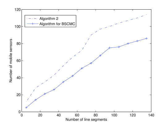
Figure 8: Comparison with respect to number of mobile sensors varying with number of line segments

Sweep period	Number of Mobile Sensors
	Algorithm for BSCMC	Algorithm 2
50	75	197
60	67	179
70	62	135
80	58	119
90	56	107
100	54	97
110	52	86
120	51	77
130	51	71
140	50	66
150	50	60

Table 2: Comparison of the number of mobile sensors to achieve sweep coverage varying sweep period for fixed number of line segments

Table 1 shows comparison of average number of mobile sensors to achieve sweep coverage for both of the algorithms varying with number of line segments. The average number of mobile sensor is calculated for 100 several executions of the algorithms with fixed sweep period 50 second. A graphical representation of the Table 1 is illustrated in Fig. 8. Table 1 and Fig. 8 show that with increasing number of line segments, the Algorithm BSCMC performs better than the Algorithm 2 with respect to average number of mobile sensors.

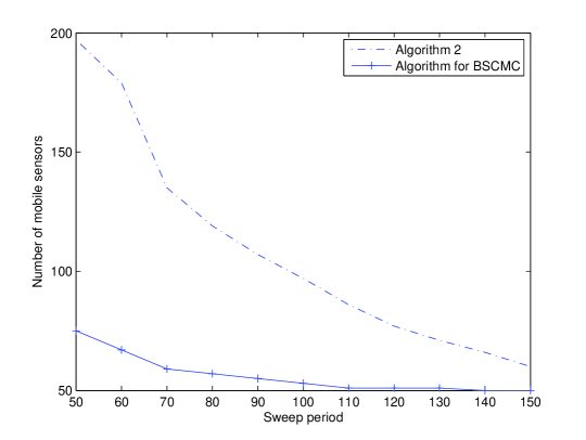
Figure 9: Comparison with respect to number of mobile sensors varying with sweep period (in second)

Table 2 shows comparison of average number of mobile sensors to achieve sweep coverage varying with the sweep periods. The average number of mobile sensor is calculated for 100 several executions of the algorithms with fixed number of line segments, which is equal to 50. A graphical representation of the Table 2 is illustrated in Fig. 9. Table 2 and Fig. 9 show that with increasing number of line segments, the difference between the average number of mobile sensors decreases. In general the Algorithm for BSCMC performs better than the Algorithm 2.

7 Conclusion

Unlike traditional coverage, in sweep coverage periodic monitoring is maintained by mobile sensors instead of continuous monitoring. There are many applications in industry, where periodic monitoring is required for identification of specific preventive maintenance. For example, periodic monitoring of electrical equipments like motors and generators is required to check their partial discharges [22].

In this paper we have introduced sweep coverage concept for barriers, where the objective is to cover finite length curves on a plane. In barrier sweep coverage, mobile sensors periodically visit all points of a set of finite length curves. For a single curve, we have solved the problem optimally. To resolve the issue of limited battery power of mobile sensors, we have proposed a solution by introducing an energy source on the plane and proposed a solution, which achieves a constant approximation factor $\frac{13}{3}$. We have proved that finding minimum number of mobile sensors to sweep cover a set of finite length curves is NP-hard and cannot be approximated within a factor of 2. For this problem we have proposed a 2-approximation algorithm for a special case, which is the best possible approximation factor. For the general problem, we propose a 5-approximation algorithm. As an application of barrier sweep coverage problems, we have defined a data gathering problem with data mules, where the concept of barrier sweep coverage is applied for gathering data by utilizing minimum number of data mules. A 3-approximation algorithm is proposed to solve the problem. In future we want to investigate the sweep coverage problems in presence of obstacles. There would be another possible extension of this work a plane, where the surface might be uneven.

References

- [1] Giuseppe Anastasi, Marco Conti, and Mario Di Francesco. Data collection in sensor networks with data mules: an integrated simulation analysis. In IN: PROC. OF IEEE ISCC, 2008.
- [2] Maxim A. Batalin and Gaurav S. Sukhatme. Multi-robot dynamic coverage of a planar bounded environment. In Technical Report, CRES-03-011, 2002.
- [3] Mihaela Cardei and Ding-Zhu Du. Improving wireless sensor network lifetime through power aware organization. Wireless Networks, 11(3):333–340, 2005.
- [4] Güner D. Çelik and Eytan Modiano. Dynamic vehicle routing for data gathering in wireless networks. In CDC, pages 2372–2377, 2010.
- [5] Ai Chen, Santosh Kumar, and Ten H. Lai. Designing localized algorithms for barrier coverage. In Proceedings of the 13th Annual ACM International Conference on Mobile Computing and Networking, MobiCom ’07, pages 63–74, New York, NY, USA, 2007. ACM.
- [6] N. Christofides. Worst-case analysis of a new heuristic for the travelling salesman problem. Technical Report 388, Graduate School of Industrial Administration, Carnegie Mellon University, 1976.
- [7] Hung-Chi Chu, Wei-Kai Wang, and Yong-Hsun Lai. Sweep coverage mechanism for wireless sensor networks with approximate patrol times. Ubiquitous, Autonomic and Trusted Computing, Symposia and Workshops on, 0:82–87, 2010.
- [8] Jurek Czyzowicz, Leszek Gasieniec, Adrian Kosowski, and Evangelos Kranakis. Boundary patrolling by mobile agents with distinct maximal speeds. In Camil Demetrescu and MagnúsM. Halldórsson, editors, Algorithms ESA 2011, volume 6942 of Lecture Notes in Computer Science, pages 701–712. Springer Berlin Heidelberg, 2011.
- [9] Junzhao Du, Yawei Li, Hui Liu, and Kewei Sha. On sweep coverage with minimum mobile sensors. In Proceedings of the 2010 IEEE 16th International Conference on Parallel and Distributed Systems, ICPADS ’10, pages 283–290, Washington, DC, USA, 2010. IEEE Computer Society.
- [10] Adrian Dumitrescu and Csaba D. Tóth. Computational geometry column 59. SIGACT News, 45(2):68–72, June 2014.
- [11] Barun Gorain and Partha Sarathi Mandal. Approximation algorithms for sweep coverage in wireless sensor networks. Journal of Parallel and Distributed Computing, 74(8):2699 – 2707, 2014.
- [12] Barun Gorain and Partha Sarathi Mandal. Approximation algorithm for sweep coverage on graph. Inf. Process. Lett., 115(9):712–718, 2015.
- [13] Barun Gorain and Partha Sarathi Mandal. Solving energy issues for sweep coverage in wireless sensor networks. Discrete Applied Mathematics, pages –, 2016.
- [14] Yu Gu, Yusheng Ji, Jie Li, and Baohua Zhao. Fundamental results on target coverage problem in wireless sensor networks. In GLOBECOM’09, pages 1–6, 2009.
- [15] Akitoshi Kawamura and Yusuke Kobayashi. Fence patrolling by mobile agents with distinct speeds. Distributed Computing, 28(2):147–154, 2015.
- [16] Santosh Kumar, Ten H. Lai, and Anish Arora. Barrier coverage with wireless sensors. In Proceedings of the 11th Annual International Conference on Mobile Computing and Networking, MobiCom ’05, pages 284–298, New York, NY, USA, 2005. ACM.
- [17] Liron Levin, Alon Efrat, and Michael Segal. Collecting data in ad-hoc networks with reduced uncertainty. Ad Hoc Networks, 17:71–81, 2014.
- [18] Liron Levin, Michael Segal, and Hanan Shpungin. Optimizing performance of ad-hoc networks under energy and scheduling constraints. In WiOpt, pages 11–20, 2010.
- [19] Mo Li, Wei-Fang Cheng, Kebin Liu, Yunhao Liu, Xiang-Yang Li, and Xiangke Liao. Sweep coverage with mobile sensors. IEEE Trans. Mob. Comput., 10(11):1534–1545, 2011.
- [20] Benyuan Liu, Olivier Dousse, Jie Wang, and Anwar Saipulla. Strong barrier coverage of wireless sensor networks. In Proceedings of the 9th ACM International Symposium on Mobile Ad Hoc Networking and Computing, MobiHoc ’08, pages 411–420, New York, NY, USA, 2008. ACM.
- [21] Mingming Lu, Jie Wu, Mihaela Cardei, and Minglu Li. Energy-efficient connected coverage of discrete targets in wireless sensor networks. In ICCNMC’05, pages 43–52, 2005.
- [22] G. Paoletti and A. Golubev. Partial discharge theory and applications to electrical systems. In Pulp and Paper, 1999. Industry Technical Conference Record of 1999 Annual, pages 124–138, 1999.
- [23] A. Saipulla, C. Westphal, Benyuan Liu, and Jie Wang. Barrier coverage of line-based deployed wireless sensor networks. In INFOCOM 2009, IEEE, pages 127–135, April 2009.
- [24] Mana Saravi and Bahareh J. Farahani. Distance constrained deployment (DCD) algorithm in mobile sensor networks. In Proceedings of the 2009 Third International Conference on Next Generation Mobile Applications, Services and Technologies, NGMAST ’09, pages 435–440, Washington, USA, 2009. IEEE Computer Society.
- [25] Rahul C. Shah, Sumit Roy, Sushant Jain, and Waylon Brunette. Data mules: modeling and analysis of a three-tier architecture for sparse sensor networks. Ad Hoc Networks, 1(2-3):215–233, 2003.
- [26] Li Shu, Ke-wei Cheng, Xiaowen Zhang, and Jiliu Zhou. Periodic sweep coverage scheme based on periodic vehicle routing problem. JNW, 9(3):726–732, 2014.
- [27] Chao Wang and Huadong Ma. Data collection in wireless sensor networks by utilizing multiple mobile nodes. In Mobile Ad-hoc and Sensor Networks (MSN), 2011 Seventh International Conference on, pages 83–90, Dec 2011.
- [28] Guiling Wang, Guohong Cao, and T. LaPorta. A bidding protocol for deploying mobile sensors. In Proceedings. 11th IEEE International Conference on Network Protocols (ICNP 2003), pages 315 – 324, Nov. 2003.
- [29] Min Xi, Kui Wu, Yong Qi, Jizhong Zhao, Yunhao Liu, and Mo Li. Run to potential: Sweep coverage in wireless sensor networks. In ICPP, pages 50–57, 2009.
- [30] Guanqun Yang and Daji Qiao. Barrier information coverage with wireless sensors. In INFOCOM, pages 918–926. IEEE, 2009.
- [31] Meng Yang, Donghyun Kim, Deying Li, Wenping Chen, Hongwei Du, and Alade O. Tokuta. Sweep-coverage with energy-restricted mobile wireless sensor nodes. In Kui Ren, Xue Liu, Weifa Liang, Ming Xu, Xiaohua Jia, and Kai Xing, editors, WASA, volume 7992 of Lecture Notes in Computer Science, pages 486–497. Springer, 2013.