Topological Kondo insulators in one dimension: Continuous Haldane-type ground-state evolution from the strongly-interacting to the non-interacting limit

Abstract

We study, by means of the density-matrix renormalization group (DMRG) technique, the evolution of the ground state in a one-dimensional topological insulator, from the non-interacting to the strongly-interacting limit, where the system can be mapped onto a topological Kondo-insulator model. We focus on a toy model Hamiltonian (i.e., the interacting “$sp$-ladder” model), which could be experimentally realized in optical lattices with higher orbitals loaded with ultra-cold fermionic atoms. Our goal is to shed light on the emergence of the strongly-interacting ground state and its topological classification as the Hubbard-$U$ interaction parameter of the model is increased. Our numerical results show that the ground state can be generically classified as a symmetry-protected topological phase of the Haldane-type, even in the non-interacting case $U=0$ where the system can be additionally classified as a time-reversal $\mathbb{Z}_{2}$-topological insulator, and evolves adiabatically between the non-interacting and strongly interacting limits.

Introduction. The search for novel states of matter with nontrivial topology has become an exciting pursuit in condensed matter physics (Kane and Mele, 2005; Bernevig and Hughes, 2013; Hasan and Kane, 2010; Qi and Zhang, 2011), and have opened a promising new path towards fault-tolerant quantum computation (Nayak et al., 2008). An important theoretical progress has been made in recent years with a complete classification of insulating/superconducting topological free-fermion systems in terms of dimensionality and global symmetries of the Hamiltonian (Altland and Zirnbauer, 1997; Kitaev, 2009; Ryu et al., 2010). However, a key open question is how to extend this classification to interacting phases. For instance, it has been shown recently that in one spatial dimension (1D) interactions can completely modify the free-fermion topological classification (Fidkowski and Kitaev, 2010; Turner et al., 2011).

Topological Kondo insulators (TKIs) are a particular class of strongly-interacting heavy-fermion materials where this question naturally appears (Dzero et al., 2010, 2012, 2015). In Refs. (Dzero et al., 2010, 2012, 2015), it was suggested that samarium hexaboride (SmB₆), a narrow-gap Kondo insulator known for more than 40 years, should be reinterpreted as a TKI, generating a great deal of excitement. However, despite the existence of supporting evidence for the TKI scenario (Wolgast et al., 2013; Zhang et al., 2013; Xu et al., 2014; Kim et al., 2014), the nature of the insulating state of SmB₆ has recently been put under debate (Tan et al., 2015; Wakeham et al., 2016; Laurita et al., 2016; Biswas et al., 2017), and more theoretical and experimental work is needed to fully understand it.

From a different perspective, atomic, molecular and optical (AMO) systems have become an important tool to study strongly-correlated topological phases, thanks to the recent progress in experimental techniques. In particular, cold atoms loaded into higher-orbital optical lattices with nontrivial band-structure topology have opened a new front in the pursuit of novel phases of matter, both from the theoretical (Isacsson and Girvin, 2005; Kuklov, 2006; Sun et al., 2012; Li et al., 2013; Chen et al., 2016) and the experimental (Müller et al., 2007; Wirth et al., 2011; Soltan-Panahi et al., 2012; Ölschläger et al., 2011) point of view. The topology of $p$-orbital bands combined with interaction effects leads to interesting physical systems (Lewenstein and Liu, 2015), among which a predicted “Chern Kondo insulating” phase in 2D optical lattices (Chen et al., 2016), and robust topological states in strongly interacting ladder-like optical lattices in 1D (Li et al., 2013), could be relevant to understand the nature of the insulating state of TKIs.

As an attempt to better understand the properties of bulk TKIs, Alexandrov and Coleman proposed recently a 1D toy-model for a TKI (i.e., a “$p$-wave” Kondo-Heisenberg lattice) (Alexandrov and Coleman, 2014). Analyzing the symmetries of this model in the mean-field approximation, these authors argued that it should be classified as a class-D insulator, according to the free-fermion topological classes (Altland and Zirnbauer, 1997; Kitaev, 2009; Ryu et al., 2010). Soon after, using Abelian bosonization, density matrix renormalization group (DMRG), and quantum Monte Carlo techniques, the ground state of 1DTKIs was identified as a Haldane-type insulating phase (Lobos et al., 2015; Mezio et al., 2015; Hagymási and Legeza, 2016; Lisandrini et al., 2016; Zhong et al., 2016), which has no evident connection to the non-interacting topological classes of Refs. (Altland and Zirnbauer, 1997; Kitaev, 2009; Ryu et al., 2010). This result came as a surprise, as the Haldane phase is a paradigmatic topological phase in one dimension, originally associated to the spin-1 antiferromagnetic chain, and is the simplest example of a symmetry-protected topological (SPT) phase (Affleck et al., 1987, 1989; Kennedy and Tasaki, 1992; Pollmann et al., 2010, 2012). More importantly, the results in Ref. (Lobos et al., 2015; Mezio et al., 2015; Hagymási and Legeza, 2016; Lisandrini et al., 2016; Zhong et al., 2016) put in evidence the risk of using mean-field approaches to interpret the properties of strongly-interacting topological phases.

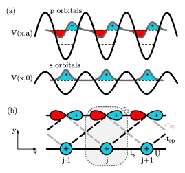
Figure 1: (color online) (a) Scheme of a realization of the $sp$-ladder model using the 2D laser potential $V\left(x,y\right)=V_{x}\sin^{2}\left(kx\right)+V_{1}\sin^{2}\left(ky\right)+V_{2}\sin^{2}\left(2ky+\phi\right)$ (Li et al., 2013). Asymmetric double-well potentials along the $\hat{y}$ axis, with $s$($p$) orbitals at position $y=0$ ($y=a$), generate a $s$-($p$-) chain in the $\hat{x}$ direction. (b) Tight-binding approximation of $V\left(x,y\right)$, where only the $s$ and $p$ orbitals are kept, generating the $sp$-ladder structure.

Motivated by these developments, in this work we study, by means of the DMRG technique, the effect of correlations on (an otherwise non-interacting) 1D $\mathbb{Z}_{2}$-topological band insulator, the 1D “$sp-$ladder” model (see Fig. 1). Specifically, we study the evolution of its ground state from the non-interacting to the strongly-interacting limit, where the model can be mapped onto the “$p$-wave” Kondo-Heisenberg model, and supports a Haldane-type ground state. We compute the entanglement entropy, entanglement spectrum, and the string-order parameter of the system, which are quantities typically used to characterize the Haldane phase (Pollmann et al., 2010, 2012), as our interaction parameter (i.e., a local Hubbard-$U$ parameter) is continuously varied. In addition, we compute the charge- and spin-excitation gaps, and the charge and spin profiles of the topologically-protected end states as a funcion of $U$. Our results show an adiabatic evolution of all ground-state properties as the interaction parameter $U$ is increased, and the absence of topological quantum phase transitions (TQPT), suggesting that the ground state can be generically classified as a symmetry-protected topological phase (SPT) of the Haldane-type, even in the non-interacting case $U=0$ where the system can be additionally classified as a time-reversal $\mathbb{Z}_{2}$-topological insulator. This finding is surprising, as these two ground states are usually considered to be qualitatively different, and naively a TQPT separating these phases could be expected. Our results are in stark contrast to the situation usually found in higher-dimensional TKIs, where the interaction $U$ destabilizes the non-interacting topological phase and induces gap-closing TQPTs at critical values of $U$ separating topologically distinct phases (Dzero et al., 2010, 2012; Chen et al., 2016; Werner and Assaad, 2013; Legner et al., 2014). Moreover, our conclusions differ from recent related studies performed on the same model using projective quantum Monte Carlo techniques (Zhong et al., 2016), where the authors conclude that the interaction $U$ breaks the adiabatic continuity of the groundstate, despite the fact that their numerical results are consistent with ours.

Theoretical model. Let us consider, for concreteness, ultracold fermions (for instance, ⁶Li or ⁴⁰K) loaded into the optical lattice of Fig. 1(a). This situation could be achieved by means of the 2D laser potential $V\left(x,y\right)=V_{x}\sin^{2}\left(kx\right)+V_{1}\sin^{2}\left(ky\right)+V_{2}\sin^{2}\left(2ky+\phi\right),$ for $V_{1},V_{2}\gg V_{x}$ (Li et al., 2013). In that limit, the system can be described as a collection of asymmetric double-wells forming two-leg ladders in the $\hat{x}$ direction, with relative depth of the two wells controlled by the phase $\phi$. We will focus on the case where the $s$ orbitals in one leg and the $p_{x}$ orbitals in the other leg are roughly degenerate. Assumming orbitals well localized at the minima of the potential, we truncate all other states in the description, and focus on the single-ladder diagram of Fig. 1(b). It can be seen that, due to their different parity, the direct overlap between $s$ and $p_{x}$ orbitals on the same rung $j$ vanishes, i.e., $\left\langle s_{j\sigma}|p_{j\sigma}\right\rangle=0$, while the overlap between next nearest-neighbor in different chains has $p-$wave symmetry, i.e., $\left\langle s_{j\sigma}|p_{j+1\sigma}\right\rangle=-\left\langle s_{j\sigma}|p_{j-1\sigma}\right\rangle$ [hence the different sign of the inter-chain hopping $t_{sp}$ in Fig.1(b)].

We therefore model an interacting open-end $sp-$ladder with $L$ sites (i.e., rungs) as $H=H_{s}+H_{p}+H_{sp}+H_{U},$ where $H_{s}=t_{s}\sum_{j=1}^{L-1}\sum_{\sigma}\left(s_{j\sigma}^{\dagger}s_{j+1\sigma}+\text{H.c.}\right)$ and $H_{p}=-t_{p}\sum_{j=1}^{L-1}\sum_{\sigma}\left(p_{j\sigma}^{\dagger}p_{j+1\sigma}+\text{H.c.}\right)$ describe the legs of the ladder, which are connected via $H_{sp}=t_{sp}\sum_{j=1}^{L}\sum_{\sigma}\left[s_{j\sigma}^{\dagger}\left(p_{j+1\sigma}-p_{j-1\sigma}\right)+\text{H.c.}\right]$. The operator $s_{j\sigma}$ ($p_{j\sigma}$) annihilates a fermion with spin projection $\sigma$ in the $s$ ($p_{x}$) orbital at rung $j$, and $n_{j\sigma}^{s\left(p\right)}$ is the corresponding number operator. To account for the topological protected edge states, we consider open boundary conditions. Finally, the Hubbard interaction $H_{U}=U\sum_{j=1}^{L}\left(n_{j\uparrow}^{s}-\frac{1}{2}\right)\left(n_{j\downarrow}^{s}-\frac{1}{2}\right)$, which can be physically produced and controlled in a cold-fermion setup via Feshbach resonances, is assumed to exist only in the $s-$orbitals, as we eventually want to make contact with the physics of strongly-interacting Kondo insulators. This model is closely related to the (interacting) Shockely-Tamm (Shockley, 1939; Tamm, 1932) or Creutz-Hubbard ladder (Creutz, 1999; Jünemann et al., 2016) models, and is such that when $U=0$ it describes a time-reversal invariant $\mathbb{Z}_{2}$-topological band-insulator (Kane and Mele, 2005; Zhong et al., 2016), and when $U\gg t_{s},t_{sp}$ it can be mapped via a canonical transformation onto the 1D $p-$wave Kondo-Heisenberg model, with Kondo and Heisenberg exchange couplings $J_{K}=8t_{sp}^{2}/U$ and $J_{K}=4t_{s}^{2}/U$, respectively, and where the ground state is a SPT phase of the Haldane type (Mezio et al., 2015). In what follows, $t_{s}$ will be the unit of energies.

We now focus on the ground-state properties of $H$ at, or near to, half-filling, i.e., when there are $N=2L$ fermions in the system. For $U=0$, the topological features can be easily understood in the “flat-band” case $t_{s}=t_{p}=t_{sp}=t$, where $H$ can be written in terms of the new fermionic operators $\gamma_{\pm,j\sigma}=\frac{1}{\sqrt{2}}\left(s_{j\sigma}\pm p_{j\sigma}\right)$ as $H_{\text{flat}}=2t\sum_{j=1,\sigma}^{L-1}\left(\gamma_{-,j\sigma}^{\dagger}\gamma_{+,j+1\sigma}+\text{H.c.}\right)$ (see Supplemental Material A). The topologically-protected edge-modes in this representation are particularly simple, corresponding to the operators $\gamma_{\alpha,\sigma}$ (with subindex $\alpha=\left\{+,1\right\}$ or $\alpha=\left\{-,L\right\}$), which drop from the Hamiltonian and therefore correspond to zero-energy modes completely localized at the ends (Creutz, 1999; Li et al., 2013; Continentino et al., 2014). In that case, we expect four degenerate states per end (e.g., the states$\left|0\right\rangle_{\alpha},\left|\uparrow\right\rangle_{\alpha},\left|\downarrow\right\rangle_{\alpha},$ and $\left|\uparrow\downarrow\right\rangle_{\alpha}$ generated by the application of $\gamma_{\alpha\uparrow}^{\dagger}$ and $\gamma_{\alpha\downarrow}^{\dagger}$). When $U$ is turned on, this 4-fold degeneracy is locally split due to the on-site repulsion, and the states $\left|0\right\rangle_{\alpha},\left|\uparrow\downarrow\right\rangle_{\alpha}$ become excited states while $\left|\uparrow\right\rangle_{\alpha},\left|\downarrow\right\rangle_{\alpha}$ span the ground state.

DMRG results. Following standard DMRG procedures (White, 1993), we have implemented the Hamiltonian $H$ with open boundary conditions, keeping $m=600$ states on every DMRG iteration, which leads to a truncation error less than $O\left(10^{-9}\right)$ and to numerical errors in the subsequent figures much smaller than symbol size.

As shown in seminal works (Turner et al., 2011; Pollmann et al., 2010, 2012; Kitaev and Preskill, 2006; Levin and Wen, 2006), the entanglement entropy and entanglement spectrum can be used to characterize SPT phases, such as the Haldane phase. In particular, it was shown that the Haldane phase is characterized by an even-degenerate entanglement spectrum (Pollmann et al., 2010). The entanglement spectrum is obtained calculating the eigenvalues $\Lambda_{i}$ of the reduced density-matrix of the system $\hat{\rho}_{L/2}$, obtained tracing out one half of the system, and the corresponding entanglement (or von Neumann) entropy is $s\left(L/2\right)=-\text{Tr}\left\{\hat{\rho}_{L/2}\ln\hat{\rho}_{L/2}\right\}=-\sum_{i}\Lambda_{i}\ln\Lambda_{i}$ (Schollwöck, 2005). A crucial observation is that the degeneracy of the entanglement spectrum in a SPT phase cannot change without a bulk phase transition, where the nature of the ground state must change abruptly or where the correlation length must diverge due to the closure of a bulk gap (Turner et al., 2011). Moreover, the occurrence of a gap-closing TQPT separating topologically distinct phases should be accompanied by a logarithmic divergence of the entanglement entropy $s\left(L/2\right)\sim k\ln\left(L\right)+\text{const}$ at the critical point (Schollwöck, 2005).

In order to investigate for the existence of a bulk TQPT, we have computed: (a) the entanglement spectrum, (b) the entanglement entropy, (c) the charge- and spin-excitation gaps, and (d) the string order parameter of $sp-$ladders ranging from $L=20$ to 80, total number of fermions $N=\left(N^{\uparrow}+N^{\downarrow}\right)$, and total spin projection $S^{z}=\frac{1}{2}\left(N^{\uparrow}-N^{\downarrow}\right)$. Unless otherwise stated, we have used the parameters $t_{p}/t_{s}=\pi/10$, $t_{sp}/t_{s}=1$, in order to recover the results obtained for the $p$-wave Kondo-Heisenberg model studied in Ref. (Mezio et al., 2015) when $U\rightarrow\infty$. In Fig. 2(a) we show the evolution of the largest eigenvalues $\Lambda_{i}$ of the entanglement spectrum and in Fig. 2(b) the corresponding entropy $s\left(L/2\right)$. The charge- and spin-excitation gaps in the 1D bulk, defined as $\Delta_{\text{c}}\left(L\right)\equiv E_{0}\left(S^{z}=0,N=2L+4\right)-E_{0}\left(S^{z}=0,N=2L\right)$ and $\Delta_{\text{s}}\left(L\right)\equiv E_{0}\left(S^{z}=2,N=2L\right)-E_{0}\left(S^{z}=0,N=2L\right)$, respectively, where $E_{0}\left(S^{z},N\right)$ is the energy of the ground state $\left|\psi_{0}\left(S^{z},N\right)\right\rangle$, are shown in Fig. 2(c), where we have extracted the values of $\Delta_{\text{c}}\left(L\right)$ and $\Delta_{\text{s}}\left(L\right)$ in the thermodynamic limit $L\rightarrow\infty$ by the means of a finite-size scaling.

All of our results show a smooth and continuous evolution as $U$ is varied, without any signature of a TQPT as the system size is increased. In particular, the even-degenerate character of the entanglement spectrum is preserved [see Fig. 2(a)], despite the continuous breaking of the degeneracy existing at $U=0$ into two branches, presumably corresponding to lower-lying spin and higher-lying charge degrees of freedom. This is substantiated by the behavior of $\Delta_{\text{c}}\left(L\right)$ and $\Delta_{\text{s}}\left(L\right)$ shown in Fig. 2(c), where the degeneracy of the charge and spin sectors at $U=0$ is broken in a continuous fashion, and excitations become fractionalized into low-lying spin and high-lying charge excitations. The entanglement entropy $s\left(L/2\right)$, shown in Fig. 2(b), does not present any divergence as the system size increases, and is bounded from below by $s_{\text{min}}=\ln\left(2\right)\simeq 0.693$, the entropy of the Affleck-Kennedy-Lieb-Tasaki (AKLT) state corresponding to the 2 degenerate end-states $\left|\uparrow\right\rangle,\left|\downarrow\right\rangle$ (Pollmann et al., 2010). At $U=0$, a similar lower-bound is given by the flat-band state, i.e., $s_{\text{min}}=\ln\left(4\right)\simeq 1.386$, related to the 4 aforementioned degenerate end states.

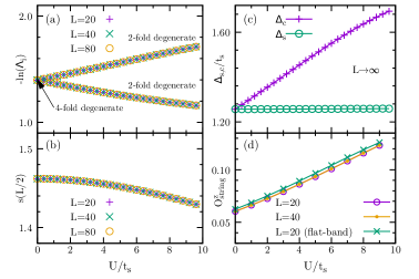
Figure 2: (color online) (a) Largest eigenvalues $\Lambda_{i}$ of the entanglement spectrum as a function of $U$, for different lattice sizes. (b) Entanglement entropy of the reduced density matrix, $s\left(L/2\right)$, as function of $U$ for different lattice sizes. (c) Spin and charge gap extrapolated to the thermodynamic limit $L\rightarrow\infty$. (d) String order parameter $\mathcal{O}_{\text{string}}^{z}$ as function of $U$ for different system-sizes.

In order to further clarify the crossover, we have calculated the string correlator $\mathcal{O}_{\text{string}}^{z}\left(l-m\right)=-\left\langle T_{l}^{z}e^{i\pi\sum_{l<j<m}T_{j}^{z}}T_{m}^{z}\right\rangle$, a non-local quantity that characterizes the breaking of the $Z_{2}\times Z_{2}$ hidden symmetry of the Haldane phase (Kennedy and Tasaki, 1992). In Fig. 2(d) we plot the string order parameter $\mathcal{O}_{\text{string}}^{z}$ (i.e., the asymptotic value of the string correlator $\mathcal{O}_{\text{string}}^{z}\left(l-m\right)$ in the 1D bulk, taking $m=L/2$ and $l=L/2+d$ in order avoid the effect of the boundaries) as a function of $U$. Again we see a smooth and continuous adiabatic crossover between the non-interacting and strongly-interacting limits. Strikingly, although this quantity has been traditionally used to characterize strongly-interacting phases, here we show that it yields a finite value for all values of $U$, even for $U=0$, where the system has no net magnetic moments due to strong charge fluctuations. This finite value of $\mathcal{O}_{\text{string}}^{z}$ for $U=0$ can be independently obtained by an analyical calculation in the flat-band case, which yields the exact result $\mathcal{O}_{\text{string}}^{z}\left(l-m\right)=1/16=0.0625$ for $\left|l-m\right|\geqslant 2$ (see Supplementary Material A). The same value is obtained with DMRG with a relative error $O\left(10^{-13}\right)$.

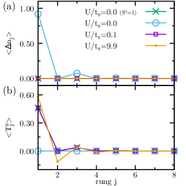
Figure 3: (color online) (a) Charge and (b) spin profiles corresponding to a ladder with $L=80$ sites and open boundary conditions, and for different values of $U$. Only the left end is shown in both cases. All profiles have been computed within the $S^{z}=0$ sector, except for $U=0$ where in addition we show the $S^{z}=+1$ profiles (represented by green crosses).

We now turn to the evolution of the topologically protected end-states. We focus on the spatial spin profile, defined as $\left\langle T_{j}^{z}\right\rangle\equiv\langle\psi_{0}\left(S^{z},N\right)|T_{j}^{z}|\psi_{0}\left(S^{z},N\right)\rangle$, where $\mathbf{T}_{j}\equiv\mathbf{s}_{j}^{s}+\mathbf{s}_{j}^{p}$, is the total spin operator on the $j$-th rung, with $\mathbf{s}_{j}^{a}\equiv a_{j\mu}^{\dagger}\left(\frac{\boldsymbol{\sigma}_{\mu,\nu}}{2}\right)a_{j\nu}$ the spin-density of $a$-fermions ($a=\left\{s,p\right\}$), and $\boldsymbol{\sigma}_{\mu,\nu}$ the vector of Pauli matrices (summation over repeated spin indices is implicit here). Invoking the $SU\left(2\right)$ spin-symmetry of the model, in what follows we will only compute the numerically simpler $z$-component. Similarly, we define the (difference in the) spatial charge profile as $\left\langle\Delta n_{j}\right\rangle\equiv\langle\psi_{0}\left(S^{z},N\right)|n_{j}|\psi_{0}\left(S^{z},N\right)\rangle-n_{0}$, where $n_{j}\equiv n_{j}^{s}+n_{j}^{p}$ is the total charge operator on rung $j$, and where we have substracted the uniform background at half-filling $n_{0}=N/L=2$. In Fig.3(a) and (b) we plot $\left\langle T_{j}^{z}\right\rangle$ and $\left\langle\Delta n_{j}\right\rangle$ for different values of $U$ at half filling $N=2L$, and for different $S^{z}$ subspaces compatible with this filling (i.e., $S^{z}=0$ and $S^{z}=\pm 1$). Note that we only show the profiles at the left end. Since the quantum numbers $S^{z}$ and $N$ must be specified in the DMRG calculation, one must be careful in the interpretation of the profiles at $U=0$, due to the 4-fold degeneracy. For $S^{z}=0$, the DMRG procedure selects a ground state with a holon and a doublon end-state (i.e., either $|0\rangle_{L}\otimes|\uparrow\downarrow\rangle_{R}$ or $|\uparrow\downarrow\rangle_{L}\otimes|0\rangle_{R}$), which has a vanishing spin profile [see light blue circles in Figs. 3(a) and (b)]. However, for $S^{z}=+1$, the end-state combination $|\uparrow\rangle_{L}\otimes|\uparrow\rangle_{R}$, which has free spin-1/2 end-states but a uniform charge profile [see green crosses in Figs. 3(a) and (b)], is selected in the ground state (com, ). However, our results are fully consistent with the presence of free-fermion end-states of a finite $\mathbb{Z}_{2}$ topological insulator. Interestingly, as soon as the interaction $U$ is turned on (see violet square symbols corresponding to $U/t_{s}=0.1$), due to the higher energy of charge excitations, the charge profile “freezes” into the uniform configuration $\left\langle n_{j}\right\rangle=n_{0}=2$, or equivalently $\left\langle\Delta n_{j}\right\rangle=0$, which is physically consistent with the adiabatic emergence of a Mott-insulating state at half-filling (Lobos et al., 2015; Mezio et al., 2015). The only surviving end-state at finite $U$ is therefore the spin end-state, which continuously crosses-over into the usual Haldane spin-1/2 end-states (Kennedy and Tasaki, 1992).

The adiabatic evolution of the ground state described here could be ideally tested in ultracold ⁶Li or ⁴⁰K gases, using recent fermionic “quantum-gas microscopes”, which allow to obtain the full spin and charge density distributions with single-atom resolution (Haller et al., 2015; Cheuk et al., 2015; Cocchi et al., 2016; Cheuk et al., 2016; Parsons et al., 2016). Thanks to their high-resolution, such techniques have been used recently to extract non-local correlation functions, such as the string-correlation function, in balanced spin-mixtures of ⁶Li atoms trapped in an asymmetric 2D optical lattice simulating a 1D Fermi-Hubbard model (Hilker et al., 2017), and could potentially be used to probe their evolution as the interaction parameter is varied using Feshbach resonances.

Conclusions. Our work sheds light on the conceptually relevant question of the classification of strongly-interacting topological phases and their connection to the free-fermion topological classes. Based on the even-degeneracy of the entanglement spectrum for all values of the interaction $U$, we conclude that the ground state of the system can be generically classified as a SPT Haldane-type phase, even in the non-interacting case $U=0$, where the system additionally admits the usual classification as a non-interacting time-reversal $\mathbb{Z}_{2}$-topological insulator (Kane and Mele, 2005). We hope our work will trigger more theoretical and experimental research in this direction.

Acknowledgements. F.T.L, A.O.D. and C.J.G. acknowledge support from CONICET-PIP 11220120100389CO. A.M.L acknowledges support from PICT-2015-0217 of ANPCyT.

Appendix A Supplemental Material for “Topological Kondo insulators in one dimension: Continuous Haldane-type ground-state evolution from the strongly-interacting to the non-interacting limit”

Franco T. Lisandrini

Alejandro M. Lobos

Ariel O. Dobry

Claudio J. Gazza

March 17, 2024

Calculation of the string-correlator for a non-interacting flat-band $sp$ ladder

In this Supplemental Material we give details on the calculation of the string correlator $\mathcal{O}_{\text{string}}^{z}\left(l-m\right)$ in the non-interacting case $U=0$ and for flat-band parameters $t_{s}=t_{p}=t_{sp}=t$. This analytical result is striking since, despite the absence of well-defined magnetic moments in the system due to charge fluctuations, it shows that time-reversal $\mathbb{Z}_{2}$topological band-insulators can have a non-vanishing value of $\mathcal{O}_{\text{string}}^{z}\left(l-m\right)$, a quantity typically associated to the strongly interacting Haldane phase.

As mentioned in the main text, in the flat-band case the Hamiltonian reads

$$H_{\text{flat}} =t\sum_{j=1}^{L-1}\sum_{\sigma}\left[\left(s_{j\sigma}^{\dagger}-p_{j\sigma}^{\dagger}\right)\left(s_{j+1\sigma}+p_{j+1\sigma}\right)+\left(s_{j+1\sigma}^{\dagger}+p_{j+1\sigma}^{\dagger}\right)\left(s_{j\sigma}-p_{j\sigma}\right)\right]$$

$$=2t\sum_{j=1,\sigma}^{L-1}\left(\gamma_{-,j\sigma}^{\dagger}\gamma_{+,j+1\sigma}+\text{H.c.}\right),$$

where

$$\gamma_{\pm j,\sigma} =\frac{s_{j,\sigma}\pm p_{j,\sigma}}{\sqrt{2}}.$$ (1)

This Hamiltonian can be diagonalized using the basis:

$$B_{j,j+1,\sigma}^{\dagger} =\frac{\gamma_{-,j\sigma}^{\dagger}+\gamma_{+,j+1\sigma}^{\dagger}}{\sqrt{2}},$$ (2)

$$A_{j,j+1,\sigma}^{\dagger} =\frac{\gamma_{-,j\sigma}^{\dagger}-\gamma_{+,j+1\sigma}^{\dagger}}{\sqrt{2}},$$ (3)

which defines new “sites” along the diagonal rungs, and in terms of which the Hamiltonian writes

$$H_{\text{flat}}= -2t\sum_{j=1,\sigma}^{L-1}\left(A_{j,j+1,\sigma}^{\dagger}A_{j,j+1,\sigma}-B_{j,j+1,\sigma}^{\dagger}B_{j,j+1,\sigma}\right).$$

The groundstate of a system with $N=2L$ particles (i.e., half-filling), where the boundary modes are occupied with fermions $\gamma_{+,1s}^{\dagger},\gamma_{-,Ls^{\prime}}^{\dagger}$ can be expressed as

$$\left|\psi_{0}\left(s,s^{\prime}\right)\right\rangle =\left\{\prod_{j=1}^{L-1}\prod_{\sigma}A_{j,j+1,\sigma}^{\dagger}\right\}\gamma_{+,1s}^{\dagger}\gamma_{-,Ls^{\prime}}^{\dagger}\left|0\right\rangle.$$ (4)

The contribution inside the curly brackets corresponds to the gapped 1D bulk, while the last two terms are the end-states.

We now focus on the string correlator

$$\mathcal{O}_{\text{string}}^{z}\left(l-m\right) \equiv-\left\langle T_{l}^{z}e^{i\pi\sum_{l<j<m}T_{j}^{z}}T_{m}^{z}\right\rangle$$ (5)

where

$$T_{j}^{z} =\frac{n_{j,\uparrow}^{s}-n_{j,\downarrow}^{s}+n_{j,\uparrow}^{p}-n_{j,\downarrow}^{p}}{2}=\frac{n_{+,j\uparrow}-n_{+j,\downarrow}+n_{-,j\uparrow}-n_{-,j\downarrow}}{2},$$ (6)

where we have defined $n_{\pm,j\sigma}=\gamma_{\pm,j\sigma}^{\dagger}\gamma_{\pm,j\sigma}$. Since all the operators $T_{j}^{z}$ inside the expression $T_{l}^{z}e^{i\pi\sum_{l<j<m}T_{j}^{z}}T_{m}^{z}$ commute, we compute the average of $T_{l}^{z}T_{m}^{z}e^{i\pi\sum_{l<j<m}T_{j}^{z}}$ instead. Therefore, we first operate with the string on the ground state $\left|\psi_{0}\left(s,s^{\prime}\right)\right\rangle$. To that end it is useful to recall the commutation relation

$$e^{i\alpha c^{\dagger}c}c^{\dagger} =c^{\dagger}e^{i\alpha\left(c^{\dagger}c+1\right)},$$ (7)

which arises from the fermionic commutation relation $\left[c^{\dagger}c,c\right]=c^{\dagger}$. Using this relationship, we compute the effect of the string on the operator $A_{k,k+1,\sigma}$:

$$e^{i\pi\sum_{j=l+1}^{j=m-1}T_{j}^{z}}A_{k,k+1,\sigma} =\left(\frac{\gamma_{-,k\sigma}^{\dagger}e^{i\sigma\frac{\pi}{2}\left[\Theta\left(k-l-1\right)-\Theta\left(k-m+1\right)\right]}-\gamma_{+,k+1\sigma}^{\dagger}e^{i\sigma\frac{\pi}{2}\left[\Theta\left(k-l\right)-\Theta\left(k-m+2\right)\right]}}{\sqrt{2}}\right)e^{i\pi\sum_{j=l+1}^{j=m-1}T_{j}^{z}},$$ (8)

where we have defined the unit step function as:

$$\Theta\left(j\right) =\begin{cases}1&\text{for }j\geq 0,\\ 0&\text{for }j<0.\end{cases}$$

We see that the effect of the string is to introduce a phase factor $e^{i\sigma\frac{\pi}{2}}$ on every creation operator $\gamma_{\pm,k\sigma}^{\dagger}$ which verifies $l+1\leq k\leq m-1$. When both operators $\gamma_{+,k\sigma}^{\dagger}$ and $\gamma_{-,k+1\sigma}^{\dagger}$ inside the definition (3) are affected by the string, the phase factors for spin $\sigma=\uparrow$ and $\sigma=\downarrow$ compensate and cancel out as a consequence of the SU(2) symmetry of the ground state, and therefore the original operator $A_{k,k+1,\sigma}$ is restored. However, note that for $A_{l,l+1,\sigma}$ and $A_{m-1,m,\sigma}$, this is not possible and therefore after the action of the string, and a phase factor remains and we cannot restore $A_{l,l+1,\sigma}$ nor $A_{m-1,m,\sigma}$. In the thermodynamic limit $L\rightarrow\infty$, and assuming $\left|l-m\right|\geqslant 2$ with $l$ and $m$ deep in the 1D bulk, we can neglect the effect of the boundaries and therefore we can write

$$e^{i\pi\sum_{j=l+1}^{j=m-1}T_{j}^{z}}\left|\psi_{0}\left(s,s^{\prime}\right)\right\rangle =\left\{\prod_{\sigma}\left(\frac{\gamma_{-,l\sigma}^{\dagger}-e^{i\sigma\frac{\pi}{2}}\gamma_{+,l+1\sigma}^{\dagger}}{\sqrt{2}}\right)\left(\frac{e^{i\sigma\frac{\pi}{2}}\gamma_{-,m-1\sigma}^{\dagger}-\gamma_{+,m\sigma}^{\dagger}}{\sqrt{2}}\right)\right\}$$

$$\times\left\{\prod_{j\neq\left\{l,m-1\right\}}^{L-1}\prod_{\sigma}A_{j,j+1,\sigma}^{\dagger}\right\}\gamma_{+,1s}^{\dagger}\gamma_{-,Ls^{\prime}}^{\dagger}\left|0\right\rangle,$$ (9)

where in the first brackets we have singled out the operators which cannot be restored into the original form $A_{k,k+1,\sigma}$, while in the last brackets we have regrouped the rest of the unaffected operators.

Now let us focus on the effect of $T_{l}^{z}T_{m}^{z}$. Since $T_{l}^{z}$ and $T_{m}^{z}$ are local operators acting on sites $l$ and $m$ respectively, the four operators $A_{l-1,l,\sigma}$,$A_{l,l+1,\sigma}$ and $A_{m-1,m,\sigma}$,$A_{m,m+1,\sigma}$, two of which have already been modified by the string, will be affected. Remember that we are assuming $\left|l-m\right|\geqslant 2$, otherwise some of these operators will coincide. It is convenient to single out these four terms and write (9) as

$$e^{i\pi\sum_{j=l+1}^{j=m-1}T_{j}^{z}}\left|\psi_{0}\left(s,s^{\prime}\right)\right\rangle =\left\{\prod_{\sigma}\left(\frac{\gamma_{-,l-1\sigma}^{\dagger}-\gamma_{+,l\sigma}^{\dagger}}{\sqrt{2}}\right)\left(\frac{\gamma_{-,l\sigma}^{\dagger}-e^{i\sigma\frac{\pi}{2}}\gamma_{+,l+1\sigma}^{\dagger}}{\sqrt{2}}\right)\right.$$ (10)

$$\left.\times\left(\frac{e^{i\sigma\frac{\pi}{2}}\gamma_{-,m-1,\sigma}^{\dagger}-\gamma_{+,m\sigma}^{\dagger}}{\sqrt{2}}\right)\left(\frac{\gamma_{-,m\sigma}^{\dagger}-\gamma_{+,m+1\sigma}^{\dagger}}{\sqrt{2}}\right)\right\}\times\mathbf{A}_{s,s^{\prime}}^{\dagger}\left|0\right\rangle$$ (11)

$$=\left\{\prod_{\sigma}\left(\frac{\gamma_{-,l-1,\sigma}^{\dagger}\gamma_{-,l\sigma}^{\dagger}-\gamma_{+,l,\sigma}^{\dagger}\gamma_{-,l\sigma}^{\dagger}-e^{i\sigma\frac{\pi}{2}}\gamma_{-,l-1,\sigma}^{\dagger}\gamma_{+,l+1,\sigma}^{\dagger}+e^{i\sigma\frac{\pi}{2}}\gamma_{+,l,\sigma}^{\dagger}\gamma_{+,l+1,\sigma}^{\dagger}}{2}\right)\right.$$ (12)

$$\left.\times\left(\frac{e^{i\sigma\frac{\pi}{2}}\gamma_{-,m-1,\sigma}^{\dagger}\gamma_{-,m\sigma}^{\dagger}-e^{i\sigma\frac{\pi}{2}}\gamma_{-,m-1,\sigma}^{\dagger}\gamma_{+,m+1\sigma}^{\dagger}-\gamma_{+,m\sigma}^{\dagger}\gamma_{-,m\sigma}^{\dagger}+\gamma_{+,m\sigma}^{\dagger}\gamma_{+,m+1\sigma}^{\dagger}}{2}\right)\right\}\mathbf{A}_{s,s^{\prime}}^{\dagger}\left|0\right\rangle$$ (13)

where

$$\mathbf{A}_{s,s^{\prime}}^{\dagger} =\left\{\prod_{j\neq\left\{l-1,l,m-1,m\right\}}^{L-1}\prod_{\sigma}A_{j,j+1,\sigma}^{\dagger}\right\}\gamma_{+,1s}^{\dagger}\gamma_{-,Ls^{\prime}}^{\dagger},$$ (14)

is the operator which is not affected by neither the string nor by the spin operators $T_{l}^{z}T_{m}^{z}$. Then, operating with $T_{l}^{z}T_{m}^{z}$ on the state $e^{i\pi\sum_{j=l+1}^{j=m-1}T_{j}^{z}}\left|\psi_{0}\left(s,s^{\prime}\right)\right\rangle$ and using Eq. (6) yields

$$\left|\phi_{l,m,s,s^{\prime}}\right\rangle \equiv T_{l}^{z}T_{m}^{z}e^{i\pi\sum_{j=l+1}^{j=m-1}T_{j}^{z}}\left|\psi_{0}\left(s,s^{\prime}\right)\right\rangle,$$

$$=\frac{1}{4}\left\{\left[\left(\frac{\gamma_{-,l-1,\uparrow}^{\dagger}\gamma_{-,l\uparrow}^{\dagger}-2\gamma_{+,l,\uparrow}^{\dagger}\gamma_{-,l\uparrow}^{\dagger}+e^{i\frac{\pi}{2}}\gamma_{+,l,\uparrow}^{\dagger}\gamma_{+,l+1,\uparrow}^{\dagger}}{2}\right)A_{l-1,l,\downarrow}^{\dagger}A_{l,l+1,\downarrow}^{\dagger}\right.\right.$$

$$\left.-A_{l-1,l,\uparrow}^{\dagger}A_{l,l+1,\uparrow}^{\dagger}\left(\frac{\gamma_{-,l-1,\downarrow}^{\dagger}\gamma_{-,l\downarrow}^{\dagger}-2\gamma_{+,l,\downarrow}^{\dagger}\gamma_{-,l\downarrow}^{\dagger}+e^{-i\frac{\pi}{2}}\gamma_{+,l,\downarrow}^{\dagger}\gamma_{+,l+1,\downarrow}^{\dagger}}{2}\right)\right]$$

$$\times\left[\left(\frac{e^{i\frac{\pi}{2}}\gamma_{-,m-1,\uparrow}^{\dagger}\gamma_{-,m\uparrow}^{\dagger}-2\gamma_{+,m\uparrow}^{\dagger}\gamma_{-,m\uparrow}^{\dagger}+\gamma_{+,m\uparrow}^{\dagger}\gamma_{+,m+1\uparrow}^{\dagger}}{2}\right)A_{m-1,m,\downarrow}^{\dagger}A_{m,m+1,\downarrow}^{\dagger}\right.$$

$$\left.\left.-A_{m-1,m,\uparrow}^{\dagger}A_{m,m+1,\uparrow}^{\dagger}\left(\frac{e^{-i\frac{\pi}{2}}\gamma_{-,m-1,\downarrow}^{\dagger}\gamma_{-,m\downarrow}^{\dagger}-2\gamma_{+,m\downarrow}^{\dagger}\gamma_{-,m\downarrow}^{\dagger}+\gamma_{+,m\downarrow}^{\dagger}\gamma_{+,m+1\downarrow}^{\dagger}}{2}\right)\right]\right\}\mathbf{A}_{s,s^{\prime}}^{\dagger}\left|0\right\rangle$$

Finally, we compute the string-order correlator as

$$\mathcal{O}_{\text{string}}^{z}\left(l-m\right) =-\left\langle\psi_{0}\left(s,s^{\prime}\right)\right|T_{l}^{z}e^{i\pi\sum_{l<j<m}T_{j}^{z}}T_{m}^{z}\left|\psi_{0}\left(s,s^{\prime}\right)\right\rangle,$$

$$=-\left\langle\psi_{0}\left(s,s^{\prime}\right)|\phi_{l,m,s,s^{\prime}}\right\rangle.$$

Using the fact that the operators $A_{j,j+1,\sigma},\ A_{j,j+1,\sigma}^{\dagger}$ anticommute with all other operators $A_{k,k+1,\sigma},\ A_{k,k+1,\sigma}^{\dagger}$ with $j\neq k$, it is easy to see that $A_{j,j+1,\sigma}$ and $A_{j,j+1,\sigma}^{\dagger}$ cancels out, since $\left(A_{j,j+1,\sigma}A_{j,j+1,\sigma}^{\dagger}\right)\left|0\right\rangle=\left|0\right\rangle$ . Then, projecting $\left|\phi_{l,m,s,s^{\prime}}\right\rangle$ onto $\left|\psi_{0}\left(s,s^{\prime}\right)\right\rangle$ yields

$$\mathcal{O}_{\text{string}}^{z}\left(l-m\right) =-\left\langle\psi_{0}\left(s,s^{\prime}\right)|\phi_{l,m,s,s^{\prime}}\right\rangle,$$

$$=-\frac{1}{4}\left\langle 0\right|\left\{\left[\left(A_{l,l+1,\uparrow}A_{l-1,l,\uparrow}\right)\left(\frac{\gamma_{-,l-1,\uparrow}^{\dagger}\gamma_{-,l\uparrow}^{\dagger}-2\gamma_{+,l,\uparrow}^{\dagger}\gamma_{-,l\uparrow}^{\dagger}+e^{i\frac{\pi}{2}}\gamma_{+,l,\uparrow}^{\dagger}\gamma_{+,l+1,\uparrow}^{\dagger}}{2}\right)\right.\right.$$

$$\left.-\left(A_{l,l+1,\downarrow}A_{l-1,l,\downarrow}\right)\left(\frac{\gamma_{-,l-1,\downarrow}^{\dagger}\gamma_{-,l\downarrow}^{\dagger}-2\gamma_{+,l,\downarrow}^{\dagger}\gamma_{-,l\downarrow}^{\dagger}+e^{-i\frac{\pi}{2}}\gamma_{+,l,\downarrow}^{\dagger}\gamma_{+,l+1,\downarrow}^{\dagger}}{2}\right)\right]$$

$$\times\left[\left(A_{m,m+1,\uparrow}A_{m-1,m,\uparrow}\right)\left(\frac{e^{i\frac{\pi}{2}}\gamma_{-,m-1,\uparrow}^{\dagger}\gamma_{-,m\uparrow}^{\dagger}-2\gamma_{+,m\uparrow}^{\dagger}\gamma_{-,m\uparrow}^{\dagger}+\gamma_{+,m\uparrow}^{\dagger}\gamma_{+,m+1\uparrow}^{\dagger}}{2}\right)\right.$$

$$\left.\left.-\left(A_{m,m+1,\downarrow}A_{m-1,m,\downarrow}\right)\left(\frac{e^{-i\frac{\pi}{2}}\gamma_{-,m-1,\downarrow}^{\dagger}\gamma_{-,m\downarrow}^{\dagger}-2\gamma_{+,m\downarrow}^{\dagger}\gamma_{-,m\downarrow}^{\dagger}+\gamma_{+,m\downarrow}^{\dagger}\gamma_{+,m+1\downarrow}^{\dagger}}{2}\right)\right]\right\}\left|0\right\rangle,$$

$$=-\left\{\frac{\left(3+e^{i\frac{\pi}{2}}\right)-\left(3+e^{-i\frac{\pi}{2}}\right)}{8}\right\}^{2},$$

$$=\frac{1}{16}\qquad(\text{for }\left|l-m\right|\geqslant 2),$$ (15)

as mentioned in the main text. It is interesting to note that all the effect of the string is encoded by the phase factors $e^{\pm i\frac{\pi}{2}}$. Should the string was not there, i.e., if we compute the spin-spin correlator

$$\mathcal{C}^{z}\left(l-m\right) \equiv\left\langle\psi_{0}\left(s,s^{\prime}\right)\right|T_{l}^{z}T_{m}^{z}\left|\psi_{0}\left(s,s^{\prime}\right)\right\rangle$$ (16)

the only change would be to replace the factors $e^{\pm i\frac{\pi}{2}}\rightarrow 1$ in the above Eq. (15) [see also Eq. (8)]. In that case, we would obtain

$$\mathcal{C}^{z}\left(l-m\right)=\left\{\frac{\left(3+1\right)-\left(3+1\right)}{8}\right\}^{2} =0, (\text{for }\left|l-m\right|\geqslant 2)$$ (17)

as expected, since the system has no net magnetic moments.

References

- Kane and Mele (2005) C. L. Kane and E. J. Mele, Phys. Rev. Lett. 95, 146802 (2005).
- Bernevig and Hughes (2013) B. A. Bernevig and T. L. Hughes, Topological Insulators and Topological Superconductors (Princeton University Press, 2013).
- Hasan and Kane (2010) M. Z. Hasan and C. L. Kane, Rev. Mod. Phys. 82, 3045 (2010).
- Qi and Zhang (2011) X.-L. Qi and S.-C. Zhang, Rev. Mod. Phys. 83, 1057 (2011).
- Nayak et al. (2008) C. Nayak, S. H. Simon, A. Stern, M. Freedman, and S. Das Sarma, Rev. Mod. Phys. 80, 1083 (2008).
- Altland and Zirnbauer (1997) A. Altland and M. R. Zirnbauer, Phys. Rev. B 55, 1142 (1997).
- Kitaev (2009) A. Kitaev, AIP Conf. Proc. 1134, 22 (2009).
- Ryu et al. (2010) S. Ryu, A. P. Schnyder, A. Furusaki, and A. W. W. Ludwig, New Journal of Physics 12, 065010 (2010).
- Fidkowski and Kitaev (2010) L. Fidkowski and A. Kitaev, Phys. Rev. B 81, 134509 (2010).
- Turner et al. (2011) A. M. Turner, F. Pollmann, and E. Berg, Phys. Rev. B 83, 075102 (2011).
- Dzero et al. (2010) M. Dzero, K. Sun, V. Galitski, and P. Coleman, Phys. Rev. Lett. 104, 106408 (2010).
- Dzero et al. (2012) M. Dzero, K. Sun, P. Coleman, and V. Galitski, Phys. Rev. B 85, 045130 (2012).
- Dzero et al. (2015) M. Dzero, J. Xia, V. Galitski, and P. Coleman, ArXiv e-prints (2015), eprint 1506.05635.
- Wolgast et al. (2013) S. Wolgast, C. Kurdak, K. Sun, J. W. Allen, D.-J. Kim, and Z. Fisk, Phys. Rev. B 88, 180405 (2013).
- Zhang et al. (2013) X. Zhang, N. P. Butch, P. Syers, S. Ziemak, R. L. Greene, and J. Paglione, Phys. Rev. X 3, 011011 (2013).
- Xu et al. (2014) N. Xu et al., Nat. Commun. 5, 4566 (2014).
- Kim et al. (2014) D. J. Kim, J. Xia, and Z. Fisk, Nat. Mater. 13, 466 (2014).
- Tan et al. (2015) B. S. Tan, Y.-T. Hsu, B. Zeng, M. Ciomaga Hatnean, N. Harrison, Z. Zhu, M. Hartstein, M. Kiourlappou, A. Srivastava, M. D. Johannes, et al., Science 349, 287 (2015).
- Wakeham et al. (2016) N. Wakeham, P. F. S. Rosa, Y. Q. Wang, M. Kang, Z. Fisk, F. Ronning, and J. D. Thompson, Phys. Rev. B 94, 035127 (2016).
- Laurita et al. (2016) N. J. Laurita, C. M. Morris, S. M. Koohpayeh, P. F. S. Rosa, W. A. Phelan, Z. Fisk, T. M. McQueen, and N. P. Armitage, Phys. Rev. B 94, 165154 (2016).
- Biswas et al. (2017) P. K. Biswas, M. Legner, G. Balakrishnan, M. C. Hatnean, M. R. Lees, D. M. Paul, E. Pomjakushina, T. Prokscha, A. Suter, T. Neupert, et al., Phys. Rev. B 95, 020410 (2017).
- Isacsson and Girvin (2005) A. Isacsson and S. M. Girvin, Phys. Rev. A 72, 053604 (2005).
- Kuklov (2006) A. B. Kuklov, Phys. Rev. Lett. 97, 110405 (2006).
- Sun et al. (2012) K. Sun, W. V. Liu, A. Hemmerich, and S. Das Sarma, Nat. Physics 8, 67 (2012).
- Li et al. (2013) X. Li, E. Zhao, and V. Liu, Nature Communications 4, 1523 (2013).
- Chen et al. (2016) H. Chen, X.-J. Liu, and X. C. Xie, Phys. Rev. Lett. 116, 046401 (2016).
- Müller et al. (2007) T. Müller, S. Fölling, A. Widera, and I. Bloch, Phys. Rev. Lett. 99, 200405 (2007).
- Wirth et al. (2011) G. Wirth, M. Ölschläger, and A. Hemmerich, Nat. Phys. 7, 147 (2011).
- Soltan-Panahi et al. (2012) P. Soltan-Panahi, D.-S. Lühmann, J. Struck, P. Windpassinger, and K. Sengstock, Nat. Phys. 8, 71 (2012).
- Ölschläger et al. (2011) M. Ölschläger, G. Wirth, and A. Hemmerich, Phys. Rev. Lett. 106, 015302 (2011).
- Lewenstein and Liu (2015) M. Lewenstein and W. V. Liu, Nat. Phys. 7, 101 (2015).
- Alexandrov and Coleman (2014) V. Alexandrov and P. Coleman, Phys. Rev. B 90, 115147 (2014).
- Lobos et al. (2015) A. M. Lobos, A. O. Dobry, and V. Galitski, Phys. Rev. X 5, 021017 (2015).
- Mezio et al. (2015) A. Mezio, A. M. Lobos, A. O. Dobry, and C. J. Gazza, Phys. Rev. B 92, 205128 (2015).
- Hagymási and Legeza (2016) I. Hagymási and O. Legeza, Phys. Rev. B 93, 165104 (2016).
- Lisandrini et al. (2016) F. T. Lisandrini, A. M. Lobos, A. O. Dobry, and C. J. Gazza, Papers in Physics 8, 080005 (2016).
- Zhong et al. (2016) Y. Zhong, Y. Liu, and H.-G. Luo, ArXiv e-prints (2016), eprint 1612.09376.
- Affleck et al. (1987) I. Affleck, T. Kennedy, E. H. Lieb, and H. Tasaki, Phys. Rev. Lett. 59, 799 (1987).
- Affleck et al. (1989) I. Affleck, T. Kennedy, E. H. Lieb, H. Tasaki, P. W. Anderson, N. Andrei, K. Furuya, J. H. Lowenstein, G. A. Baker, Jr., J. Bardeen, et al., Commun . Math. Phys. 115, 477 (1989).
- Kennedy and Tasaki (1992) T. Kennedy and H. Tasaki, Phys. Rev. B 45, 304 (1992).
- Pollmann et al. (2010) F. Pollmann, A. M. Turner, E. Berg, and M. Oshikawa, Phys. Rev. B 81, 064439 (2010).
- Pollmann et al. (2012) F. Pollmann, E. Berg, A. M. Turner, and M. Oshikawa, Phys. Rev. B 85, 075125 (2012).
- Werner and Assaad (2013) J. Werner and F. F. Assaad, Phys. Rev. B 88, 035113 (2013).
- Legner et al. (2014) M. Legner, A. Rüegg, and M. Sigrist, Phys. Rev. B 89, 085110 (2014).
- Shockley (1939) W. Shockley, Phys. Rev. 56, 317 (1939).
- Tamm (1932) I. Tamm, Physik. Zeits. Soviet Union 1, 733 (1932).
- Creutz (1999) M. Creutz, Phys. Rev. Lett. 83, 2636 (1999).
- Jünemann et al. (2016) J. Jünemann, A. Piga, S.-J. Ran, M. Lewenstein, M. Rizzi, and A. Bermudez, ArXiv e-prints (2016), eprint 1612.02996.
- Continentino et al. (2014) M. A. Continentino, H. Caldas, D. Nozadzec, and N. Trivedi, Phys. Lett. A 378, 3340 (2014).
- White (1993) S. R. White, Phys. Rev. B 48, 10345 (1993).
- Kitaev and Preskill (2006) A. Kitaev and J. Preskill, Phys. Rev. Lett. 96, 110404 (2006).
- Levin and Wen (2006) M. Levin and X.-G. Wen, Phys. Rev. Lett. 96, 110405 (2006).
- Schollwöck (2005) U. Schollwöck, Rev. Mod. Phys. 77, 259 (2005).
- (54) This is different to the results obtained in Figs. 4 and 5 in Ref. Zhong et al. (2016), where a flat charge profile is obtained for , presumably due to the statistical average performed by the quantum Monte Carlo method employed by the authors.
- Haller et al. (2015) E. Haller, J. Hudson, A. Kelly, D. A. Cotta, B. Peaudecerf, G. D. Bruce, and S. Kuhr, Nature Physics 11, 738 (2015).
- Cheuk et al. (2015) L. W. Cheuk, M. A. Nichols, M. Okan, T. Gersdorf, V. V. Ramasesh, W. S. Bakr, T. Lompe, and M. W. Zwierlein, Phys. Rev. Lett. 114, 193001 (2015).
- Cocchi et al. (2016) E. Cocchi, L. A. Miller, J. H. Drewes, M. Koschorreck, D. Pertot, F. Brennecke, and M. Köhl, Phys. Rev. Lett. 116, 175301 (2016).
- Cheuk et al. (2016) L. W. Cheuk, M. A. Nichols, K. R. Lawrence, M. Okan, H. Zhang, E. Khatami, N. Trivedi, T. Paiva, M. Rigol, and M. W. Zwierlein, Science 353, 1260 (2016).
- Parsons et al. (2016) M. F. Parsons, A. Mazurenko, C. S. Chiu, G. Ji, D. Greif, and M. Greiner, Science 353, 1253 (2016).
- Hilker et al. (2017) T. A. Hilker, G. Salomon, F. Grusdt, A. Omran, M. Boll, E. Demler, I. Bloch, and C. Gross, ArXiv e-prints (2017), eprint 1702.00642.