Multiple Populations in NGC 1851: Abundance Variations and UV Photometric Synthesis in the Washington and HST/WFC3 Systems

Abstract

The analysis of multiple populations (MPs) in globular clusters, both spectroscopically and photometrically, is key in understanding their formation and evolution. The relatively narrow Johnson U, F336W, and Stromgren and Sloan u filters have been crucial in exhibiting these MPs photometrically, but in Paper I we showed that the broader Washington C filter can more efficiently detect MPs in the test case globular cluster NGC 1851. In Paper I we also detected a double MS that has not been detected in previous observations of NGC 1851. We now match this photometry to NGC 1851’s published RGB abundances and find the two RGB branches observed in C generally exhibit different abundance characteristics in a variety of elements (e.g., Ba, Na, and O) and in CN band strengths, but no single element can define the two RGB branches. However, simultaneously considering [Ba/Fe] or CN strengths with either [Na/Fe], [O/Fe], or CN strengths can separate the two photometric RGB branches into two distinct abundance groups. Matches of NGC 1851’s published SGB and HB abundances to the Washington photometry shows consistent characterizations of the MPs, which can be defined as an O-rich/N-normal population and an O-poor/N-rich population. Photometric synthesis for both the Washington C filter and the F336W filter finds that these abundance characteristics, with appropriate variations in He, can reproduce for both filters the photometric observations in both the RGB and the MS. This photometric synthesis also confirms the throughput advantages that the C filter has in detecting MPs.

1. Introduction:

Globular clusters (GCs) have now in general been established, both photometrically and spectroscopically, to have multiple populations (MPs) with differing compositions and possibly different ages. Photometric detections of MPs in GCs include Omega Cen (Bedin et al. 2004), NGC 2808 (Piotto et al. 2007), NGC 1851 (Milone et al. 2008, hereafter M08; Lee et al. 2009a, hereafter L09; Han et al. 2009, hereafter H09; Cummings et al. 2014, hereafter Paper I), M22 (Lee et al. 2009b), M4 (Marino et al. 2008), and M2 (Lardo et al. 2013; Milone et al. 2015). In the recent Piotto et al. (2015) investigation, photometric detections of MPs are found in all 56 globular clusters observed with their special combination of filters (see below). In all of these clusters two or more red giant branches (RBGs), sub giant branches (SGBs), or even main sequences (MSs) have been observed.

NGC 1851 is a noteworthy cluster because it photometrically has two RGBs (L09; H09) and SGBs (M08; H09) plus evidence for two MSs (Paper I). Additionally, it has both a blue horizontal branch (BHB) and a red horizontal branch (RHB), where the Paper I analysis also suggested the RHB has two sequences. A further advantage to photometrically studying NGC 1851 is its very low reddening of E(B-V)=0.02 (Harris 1996), so there is no concern about the photometric effects of a large variable reddening. Spectroscopically, the two RGBs observed in NGC 1851 typically exhibit different abundances in a variety of elements, most strikingly in sodium (Na) and barium (Ba) (Villanova et al. 2010, hereafter V10; Carretta et al. 2011a, hereafter Ca11) and in nitrogen (N) (Carretta et al. 2014, hereafter Ca14). Spectroscopic observations of molecular bands in NGC 1851 show its RGB has moderate variations in CH strength but large variations in CN strengths (e.g., Lim et al. 2015), with no CN-CH anti-correlation. There is also evidence for a quadrimodal CN distribution (Campbell et al. 2012; Simpson et al. 2017). The two SGBs appear to correspond to high and low [Ba/Fe] (Gratton et al. 2012a, hereafter G12). Therefore, abundance differences likely play a key role in creating the separate sequences.

Models to explain MPs of differing abundances include 1) An initial population formed and soon after ($<$1 Gyr) a second population formed from the gas contaminated by the ejecta of the high-mass stars of the first generation (see M08; Joo & Lee 2013; Ventura et al. 2009). 2) There was a merger of two GCs of slightly different age and composition (see Ca11). The merger explanation is based on the Ca11 observation that between the two populations there is an apparent real spread in the heavy elements (e.g., iron (Fe)), not just in the light s-process elements. This spread cannot simply be explained by two distinct episodes of star formation within one cluster. 3) Enriched material was ejected from interacting massive binaries and rapidly rotating stars, and this material accreted onto the circumstellar discs of young pre-main sequence stars formed at the same time as these massive stars (Bastian et al. 2013). Unlike the other models, this model only has a single star-formation burst that creates MPs based on variations in the amount of enriched material accreted, if any at all, on each individual cluster member. This avoids the mass budget problem that plagues multiple star-formation burst models. However, a critical assessment of all current MP theories by Renzini et al. (2015) finds only the AGB pollution scenario to be possibly viable.

The key to photometrically distinguishing these MPs has been ultraviolet (UV) filters, where Sbordone et al. (2011) and Carretta et al. (2011b) have shown that realistic abundance differences in Carbon (C), Nitrogen (N), and Oxygen (O) greatly affect the UV filter bandpasses because of the strong CN, NH, and CH molecular bands present. The ground-based detections of multiple sequences have used the Johnson U, Stromgren u, or sloan u filters, but these filters are narrow and inefficient and require a significant amount of large telescope time to observe most GCs well. The Hubble Space Telescope (HST) has also been a powerful tool to photometrically analyze MPs with the F336W filter, which is comparable to Johnson U, and the F275W filter, which goes farther into the UV beyond what can be observed from the ground. Building on these filters, Milone et al. (2013) and Piotto et al. (2015) have defined the pseudo-colors C_{F275W,F336W,F410M} = (m_F275W-m_F336W)-(m_F336W-m_F410M) and the similar C_{F275W,F336W,F438W}, respectively, terming these three the ”magic trio”. These pseudo-colors take advantage of the strong OH features in F275W’s bandpass in combination with F336W’s strong sensitivity to N, and this provides a key method to photometrically distinguish most MPs. Their team is carrying out a legacy survey of Galactic globulars in the magic trio and uncovering MPs in all of them, with each GC exhibiting unique behavior (e.g., Piotto et al. 2015). F275W, however, requires the use of HST, and this far into the UV it is even more difficult to acquire the appropriate signal on the typically cool GC stars, greatly increasing the need for very limited HST time. Furthermore, given the limited lifetime of HST and because no other current or planned space facility will be sensitive below the atmospheric cutoff, it is important to investigate other filters that can uncover MPs from the ground.

In Paper I we were thus motivated to consider other available tools without these limitations. We demonstrated that the broader and more efficient Washington C filter was quite adept at photometrically detecting the NGC 1851 MPs with a ground-based 1-meter telescope and only moderate observation times. Color distribution analysis of the Washington photometry illustrated that these two populations are a dominant ($\sim$70%) bluer population (in C-T1 and C-T2) that is narrow in color and a secondary ($\sim$30%) redder but partially overlapping population that is broadly distributed in color. While the narrower band UV filters like Johnson U (H09) and Stromgren u (L09) appear to more cleanly separate the two populations in NGC 1851 into two distinct photometric branches, these two narrow and farther UV filters required five and three times as much telescope time, respectively, to perform these observations (see Paper I for more details).

For this second paper in our analysis of NGC 1851, we look at the photometric variations in the Washington C filter and how they are connected to elemental abundance variations. This is based on the detailed NGC 1851 abundance analyses in Ca11, V10, Ca14, G12, Gratton et al. (2012b, hereafter G12b), Yong et al. (2015, hereafter Y15), and Lim et al. (2015, hereafter L15). We also performed photometric synthesis and focused on the effects of variations in the three CNO abundances at constant C+N+O. Additionally, we briefly looked at the photometric effects of variations in total C+N+O, metallicity, and in He. We compare these effects in the C filter to the effects that identical variations have on the commonly used HST F336W filter, which is also very similar to Johnson U.

In Section 2 we discuss the previous abundance results, including their trends and distributions. In Section 3 we match previous abundances to out RGB photometry and analyze the abundance differences between the two branches observed in Washington C. In Section 4 we match previous abundances to the SGB and turnoff stars. In Section 5 we match previous abundances to HB stars. In Section 6 we synthesize for a representative RGB star the photometric effects that abundance variations have on C and F336W magnitudes. In Section 7 we synthesize for a representative MS star the photometric effects that abundance variations have on C and F336W magnitudes. Lastly, in Section 8 we summarize our results and conclusions.

2. Spectroscopic Abundances

There have been multiple spectroscopic studies of NGC 1851 that have focused on its RGB stars (e.g., Ca11; V10; Campbell et al. 2012; Ca14; Y15; L15), its turnoff and SGB stars (Pancino et al. 2010; Lardo et al. 2012, hereafter L12; G12), and its HB stars (G12b). All of these studies have shown that there is a broad spread of abundances (e.g., Na, O, Ba, Sr, Ni, and CN strengths) a possibly significant spread in Fe (Ca11), several abundance correlations and anti-correlations (e.g., O-Na and Ba-Sr), but unlike most globular clusters it has no CN-CH anti-correlation (Pancino et al. 2010; L12; L15; Simpson et al. 2017). In our analysis we first looked at the abundance trends and distributions for each element and used these to define the high and low abundance ranges for each element. Matching these abundances to our Washington photometry allows us to analyze the abundance variations in these stars in comparison to their placement on the photometrically observed MPs.

2.1. Abundance Trends

In each element we have searched for abundance trends with T_eff to account for either true variations in surface abundances as stars undergo evolution or those caused by potential systematics in the analysis. Therefore, the distributions across a broad range of giants can more appropriately be analyzed. Beginning with the analysis of 124 RGB stars from Ca11, we looked at the abundances of Fe, O, Na, Ca, Cr, and Ba. Across the $>$1000 K range in T_eff there is no significant correlation with T_eff for Fe, Ca, and Ba. For Na we find evidence for a minor anti-correlation of significance at greater than 99% confidence. Figure 1’s Na panel shows this trend, which is minor relative to the overall observed scatter. It is likely the result of systematics rather than a true abundance trend, but we have used this trend to divide the high and low Na abundances.

Figure 1.— The upper two panels plot [Na/Fe] and [O/Fe] versus T_eff for the RGB stars observed in Ca11. Solid data points represent detections and open-inverted triangles represent O upper limits. For Na the weak but statistically significant correlation shown is Na_cor = 1.66 – T_eff $\times$ 3.17$\times$ 10^-4. For O, in the cooler stars there is an apparent bimodal abundance distribution, but for the hotter stars the abundance trend at first appears to significantly increase. However, this is because at these hotter T_eff the oxygen spectroscopic feature becomes very weak and unmeasurable in the O-poor stars. This is illustrated by the large number of upper limits in the hotter stars. Hence, there is no intrinsic trend with T_eff and O possibly has a bimodal distribution. The lower three panels plot [Cr/Fe], [Ba/Fe], and [C/Fe] versus T_eff for the SGB stars observed in G12. For Cr and Ba the minor but statistically significant correlations shown are Cr_cor = –3.25 + T_eff $\times$ 5.27 $\times$ 10^-4 and Ba_cor = –1.17 + T_eff $\times$ 3.51 $\times$ 10^-4. Lastly, the [C/Fe] correlation is the most significant with C_cor = –4.29 + T_eff $\times$ 7.28 $\times$ 10^-4. This may represent an intrinsic T_eff correlation caused by the increasing depth of the surface convection zone along the SGB. For these four abundance sets, these correlations define our rich and poor populations for each element.

The O abundances have an apparent trend where at cooler T_eff O appears to have a bimodal distribution while at higher T_eff there appears to be no O-poor stars. Figure 1’s O panel illustrates this, including upper limits for stars without detectable O shown as open-inverted triangles. All of these upper limits are in the hotter RGB stars, and this is because the O spectral feature becomes increasingly weak in the fainter (hotter) RGB stars and was unmeasurable in the faint stars that are also O poor. Therefore, this strongly suggests that the O abundances have no significant trend with T_eff and may have a bimodal distribution across the full T_eff range, but in the fainter (hotter) giants this bimodality is washed out by errors and the inability to measure the weakest [O/Fe].

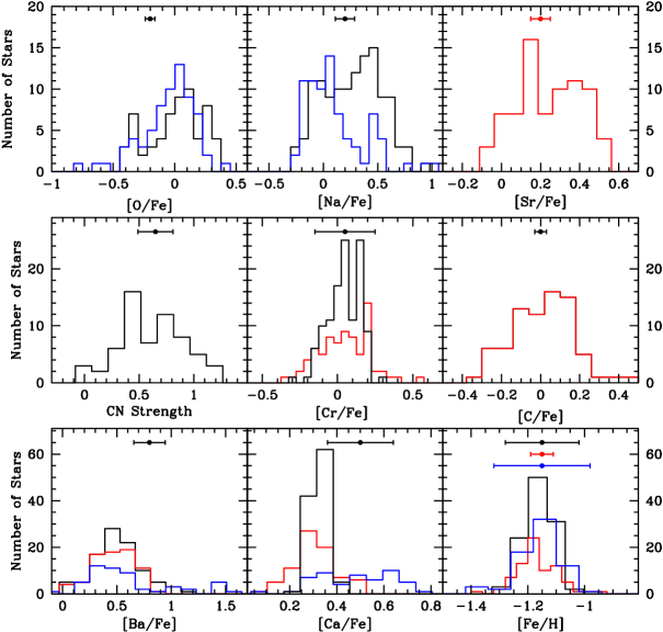
Figure 2.— The abundance distributions for various elements are shown for the RGB (Ca11; black), the SGB (G12; red), and the HB/RGB (G12b; blue). When available the typical abundance errors are shown above the distributions. For display purposes, and to directly compare the characteristics of the abundance distributions, we have applied systematic offsets to place the distributions in line with those of the RGB when possible. For [O/Fe] we applied -0.29 (G12b); no [Na/Fe] offsets; for [Cr/Fe] we applied +0.16 (G12); for [Ba/Fe] we applied -0.45 (G12) and +0.3 (G12b); for [Ca/Fe] we applied -0.09 (G12) and +0.09 (G12b); no [Fe/H] offsets.

Carretta et al. (2014, hereafter Ca14) built further on the RGB analysis in Ca11 and looked at the CN strengths of 62 of the 124 RGB stars from Ca11. In their analysis they state these CN strengths in terms of [N/Fe] with an assumed constant [C/Fe]=0. While the RGB abundances from NGC 1851 in V10 and Y15 suggest that [C/Fe] does not vary as significantly as [N/Fe] and [O/Fe] at a given magnitude, both find that [C/Fe] still does have important variations. Additionally, surface abundance evolution due to deep mixing along the RGB will cause decreasing [C/Fe] in more evolved stars. In the upper RGB, for example, [C/Fe] is more appropriately defined as $\sim$-0.8 dex rather than scaled solar. Therefore, these [N/Fe] values from Ca14 will be used as a CN strength index, but we acknowledge that these [N/Fe] values likely trace true [N/Fe] variations. Testing these CN strengths versus T_eff finds that there are no trends.

Building on these RGB abundances, we looked for similar correlations with T_eff in Fe, C, Ca, Cr, Sr, and Ba across the 77 SGB stars observed in G12 that span $\sim$800 K. As for the cases in the RGB, we again did not find any trends for [Fe/H] and [Ca/Fe]. Sr was not analyzed in the RGB, but in the SGB we did not find any meaningful trend in [Sr/Fe]. In contrast to the RGB, there is evidence for weak but statistically significant trends in [Cr/Fe] and [Ba/Fe]. Both of these trends are shown in Figure 1. Again, these are trends that are likely the result of minor systematics, and the inconsistency of the trends in the SGB and RGB supports this. In any case, we have used these trends to help define our rich and poor abundances for these elements. Lastly, the lower panel of Figure 1 shows [C/Fe] vs T_eff in the SGB from G12, which is the most scientifically interesting and strongest observed abundance-T_eff trend. [C/Fe] steeply decreases when moving from the hotter (less evolved) stars up the SGB. As G12 discuss, this trend is likely the result of mixing as the surface convection zones increase in depth along the SGB.

2.2. Abundance Distributions

Figure 2 shows the abundance distributions of nine elements or molecules of interest, where when available we have plotted the distributions derived from Ca11 (black; RGB stars), G12 (red; SGB stars), and G12b (blue; HB stars). The median abundance errors (when published) are shown above the distributions. For elements that we found correlations of significance in the previous section, we have adjusted these distributions to reflect that. Additionally, for elements that were analyzed in both Ca11 and G12, we have estimated and corrected any observed systematic differences in the distribution relative to the RGB abundances. These applied corrections are given in the caption of Figure 2. For the HB analysis, these systematics can be based directly on the overlapping samples of Ca11 and G12b, where G12b also looked at a number of RGB stars that included seven from Ca11. The calculated systematics (Ca11 minus G12b) between these RGB stars found no meaningful difference in [Fe/H], a 0.09 dex difference in [Ca/Fe], and a 0.3 dex difference in [Ba/Fe], which have been applied in Figure 2. For [Na/Fe] and [O/Fe] the measured systematics are even larger at 0.31 and -0.56, respectively, but in Figure 2 these resulted in clear offsets between the observed distributions. For display purposes we instead matched up the distributions with no offset in [Na/Fe] and a -0.29 offset in [O/Fe]. While the [Na/Fe] and [O/Fe] differences between the RGB and HB may be real, for the purposes of this paper the cause of this systematic is not important.

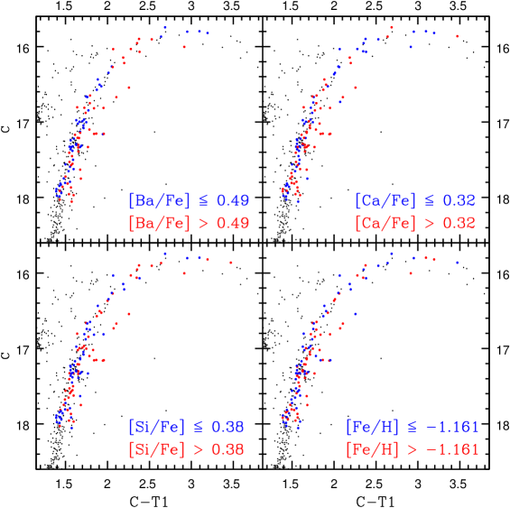
Figure 3.— Matches of the Ca11 and V10 abundances to our Washington photometry for Ba, Ca, Si, and Fe. In each panel the analyzed stars rich in the element labeled are shown in red while the analyzed stars poor in that element are shown in blue. The abundance ranges are defined in each panel. The photometric matches find that stars poor in Ba (and less so in Ca or Si) are consistently found to fall along the blue branch of the RGB. In contrast, the stars that are rich in either Ba, Ca, or Si, are broadly distributed in color and fall along both the blue branch as well as create the sparse red branch of the RGB. The photometric difference between the Fe-rich and Fe-poor populations are not significant.

Looking at the distributions themselves, while errors and number statistics limit the significance of some of these abundance variations, the distributions of many of the elements suggest a significant spread beyond that caused by errors. Furthermore, some abundances even suggest a bimodal distribution (O, Na, Sr). The significance of these bimodalities are further strengthened by being observed in more than one study. For example, the smaller sample of 15 RGB stars from V10, not shown here, also shows a clear bimodality in Sr. The distribution of [O/Fe] is of particular interest with (as seen in Figure 1) a small population of very O-poor RGB stars from Ca11, but here we also see that this population exists in the HB and RGB analysis of G12b, strengthening the significance of this bimodality.

3. Matching Red Giant Branch Abundances to Photometry

3.1. Characterizing the Red Giant Branch Abundances

Figure 3 matches the Ca11 abundances of Ba, Ca, Si, and Fe to our Paper I photometry of the two RGB populations in NGC 1851. We have also supplemented these abundances with three RGB star abundances from V10, which have been systematically adjusted to be consistent with the Ca11 abundances. This finds that the two photometric RGB branches have different abundance characteristics in Ba and Ca, but any differences are less clear in Si and Fe. The Ba-poor stars and the Ca-poor primarily fall tightly along the blue RGB, while the Ba-rich and Ca-rich stars are more widely distributed and cover both the blue and red RGB. This photometric abundance distribution, most clearly observed in Ba, is remarkably similar to the two photometric populations observed in Paper I. Based solely on photometric color distribution analysis, we found that the C filter does not distinctly separate the MPs but creates a narrow blue population and an overlapping broader and redder second population.

A more robust statistical analysis of these population distributions can be performed with a Kolmogorov-Smirnov test (KS-test). In Figure 4 we look at the photometric C-T1 colors these stars relative to a mean RGB trend, and we present the cumulative distributions of the rich and poor populations for each element. The KS-test looks at the measurement of the greatest separation (D) between each distribution, and based on the population sizes this provides the significance (p-value) of whether or not these different abundances correlate with distinct colors. As is common we adopt p-values of $<$0.05 as representative of a statistically significant difference in color distributions between the two populations (i.e., that we can reject the null hypothesis that these abundance groups are derived from the same color distribution).

In Table 1 we give the KS-test statistics for each element and molecule analyzed (see Figures 3 to 6 for display of most of these elements and molecules). This finds that in Figures 3 and 4 the distinct color distributions based on abundance in Ba and Ca are statistically significant. While Si shows a weaker distinction, the differences are still significant. In contrast to this, the comparison of the Fe-rich and Fe-poor populations from Ca11 in the RGB gives a D of 0.2379 and p-value 0.078. Therefore, while this does not rule out the significance of this possible [Fe/H] spread observed by Ca11, Fe does not correlate well with the different photometric branches. Ca11 also found this when they matched the different [Fe/H] to the Stromgren photometry by Calamida et al. (2007), where both the metal-rich and metal-poor stars showed similar double RGBs. This is the foundation for their argument that NGC 1851 was formed from the merger of two different clusters.

Table 0 - Abundance Distribution KS-Test Statistics
Element Poor Count Rich Count D p-value
Ba 51 47 0.4293 0.000
Ca 53 56 0.3133 0.007
Si 54 54 0.2593 0.043
Fe 56 53 0.2379 0.078
Cr 53 45 0.1379 0.711
Mg 48 57 0.2007 0.218
O 36 36 0.3333 0.028
Na 49 57 0.3863 0.000
CN 47 42 0.5228 0.000
CH 27 27 0.2222 0.466

Table 1For each element or molecule we matched to the RGB, we give the corresponding number of rich and poor stars, (D) the greatest separation between the cumulative distributions of the two populations, and the corresponding p-value where we adopt p$<$0.05 as significant.

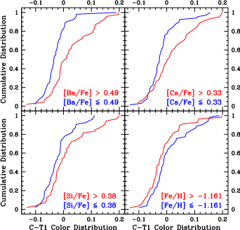
Figure 4.— We analyze the statistical properties of the photometric abundance distributions in Figure 3. Adopting the same abundance groups (and color schemes), we look at how the cumulative distributions compare between the rich and poor populations for each element in C-T1 color space. We derive relative C-T1 colors by fitting the mean RGB trend with the relation of C-T1=507.974-T1$\times$129.2119+T1${}^{2}\times$12.44539-T1${}^{3}\times$0.5351378+T1${}^{4}\times$0.00864987.

In the upper panels of Figure 5 we match the key elements of O and Na (from Ca11 supplemented with V10) to the RGB. Like with Ba, Na clearly shows that nearly all Na-poor stars are consistent with the narrow blue branch while the Na-rich population is broadly spread covering the blue branch but also creating the red branch. We similarly find a distinct distribution between the O-poor and O-rich stars, but for this element the blue branch is primarily O-rich (not poor like with Ba and Na) while the red branch is predominantly created by O-poor stars. Looking in more detail at [O/Fe], as we noted in Section 2.1, its abundance may have a bimodal distribution. Much of this is washed out, however, by the difficult measurement of O in the faint and hotter RGB stars, which appears to have been unmeasurable in the O-poor stars in this regime. Qualitatively consistent with this idea is that none of the faint red-branch RGB stars that were analyzed in Ca11 have O detections in Figure 3; only the faint blue-branch RGB stars have O detections. In the upper panels of Figure 6 we look at the cumulative distributions of the O and Na abundance populations from Figure 5.

Why do these different abundance populations have such different photometric characteristics? As described, the “red RGB branch” is composed of second population stars but many second population stars also fall on the “blue RGB branch”. On average the second population stars that fall on the red RGB branch are moderately more Ba-rich, Na-rich, or O-poor than the second population stars that fall on the blue RGB branch. However, several of the most Ba-rich, Na-rich, or O-poor stars still fall on the blue RGB branch. This suggests it is not our adopted definitions of the abundance groups that create these overlapping distributions. Ca11 similarly found photometrically overlapping populations in matches of their abundances to the Stromgren photometry of L09, and this suggests that MPs can create similar photometric characteristics in the C and Stromgren u filters.

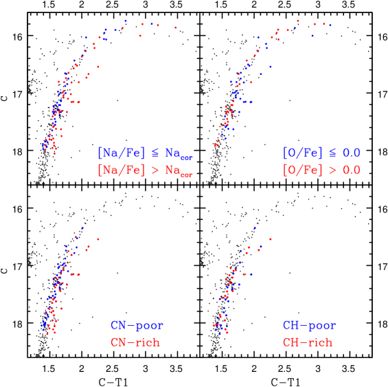
Figure 5.— Matches of the Ca11 and V10 abundances to our Washington photometry for Na, and O, and matches of the CN and CH bands strengths from Ca14 and L15 to our Washington photometry. In each panel the analyzed stars rich in the element labeled are shown in red while the analyzed stars poor in that element are shown in blue. The O abundance ranges are defined in the panel. As seen in Figure 1, we use the [Na/Fe] correlation with T_eff to define the Na-rich and Na-poor stars. For CN the CN-poor stars are [N/Fe]$\leq$-0.05 for the Ca14 abundances or $\delta$CN$\leq$0 for the L15 abundances, and the CN-rich stars are [N/Fe]$>$-0.05 for the Ca14 abundances or $\delta$CN$>$0 for the L15 abundances. For CH the CH-rich stars are $\delta$CH$>$0 and the CH-poor stars are $\delta$CH$<$0 from L15. Like with Ba, the photometric matches find that stars poor in either Na or CN, or those that are rich in O, are consistently found to fall along the blue branch of the RGB. In contrast, the stars that are rich in either Na or CN, or those that are poor in O, are broadly distributed in color and fall along both the blue branch as well as create the sparse red branch of the RGB. The photometric difference between the CH-rich and CH-poor stars are not significant.

Carretta et al. (2011b, hereafter Ca11b), Ca11, and more recently Ca14 have analyzed why the population that is typically poor in light s-process elements is photometrically very narrow and the population that is typically rich in light s-process elements is very broad in color and centered redward in the Stromgren filters. Ca11b originally suggested a model based purely on variations in CNO abundances where the two stellar populations can be defined as C-normal and C-rich, which can recreate the general observed photometric characteristics. However, in this paper we have focused instead on a photometrically similar model of two populations that are distinctly N-normal and N-rich in abundance. This is based on four recent abundance analyses: First, in Ca14 the redder RGB stars were found to be distinctly CN-rich and the bluer RGB stars were primarily CN-weak. Supplementing this finding, the analysis by V10 suggested that the most clear abundance distinction between the giants in NGC 1851 are a Ba-rich and a Ba-poor population, but these Ba-rich and Ba-poor populations were also found to be N-rich/O-poor and N-normal/O-rich, respectively. In V10 the two populations had a difference in [N/Fe] nearly as significant as [Ba/Fe]. Additionally, while the total V10 sample has moderate variations in [C/Fe], the Ba-rich and Ba-poor populations themselves show no significant difference in their mean [C/Fe]. The recent analysis by Y15 also looked at CNO in the two RGBs of NGC 1851 for 11 stars, and they find the same qualitative details as previous analyses. Lastly, L15 looked directly at CN and CH band strengths in 62 RGB stars from NGC 1851. While they found a moderate spread in CH band indexes, they found a significant spread in the observed CN band indexes. Based on this, N (and O) appears to be a key element in distinguishing the populations, which is expected due to the strong molecular bands sensitive to N in the UV.

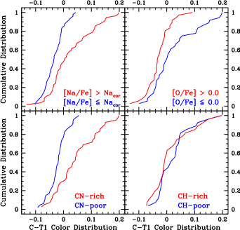
Figure 6.— We analyze the statistical properties of the photometric abundance distributions in Figure 5. Adopting the same abundance groups (and color schemes) we look at how the cumulative distributions compare between the rich and poor populations for each element or molecule in C-T1 color space, adopting the same mean RGB trend as in Figure 4.

Another key factor to consider between the abundances of the two RGB branches is whether the observed variations in C, N, and O still result in a constant total C+N+O abundance. The analysis in V10 found that both populations did have a consistent log $\epsilon$(CNO)$\sim$8.00³. Comparison of V10 to the results of Y15 finds encouraging consistency in the blue RGB, but the Y15 analysis of the red RGB stars finds they are nearly a factor of 10 ($\sim$0.9 dex) richer in N than the blue RGB. V10 only found them twice as rich in N ($\sim$0.35 dex) with respect to the blue RGB. A comparison of the CN strengths in Ca14 similarly suggests the CN-rich stars are $\sim$0.4 dex richer in N. This far more significant increase in N found by Y15 also results in a distinct log $\epsilon$(CNO) abundance between the two branches, with the red RGB branch being $\sim$0.5 dex richer. In our synthetic magnitude analysis (see Sections 6 and 7) we have adopted a constant log $\epsilon$(CNO) of 8.0, but consistent with Y15 we also briefly consider the effects of a significant increase in [N/Fe] in the red branch that results in a distinct log $\epsilon$(CNO) of 8.5 for the red.

To look more directly at the effects of CNO and the corresponding molecular bands, we first use the CN strengths from Ca14 (represented by [N/Fe]) and L15 (represented by $\delta$CN). These CN band strengths are useful because they (with the CH and NH bands) are the primary cause of the observed photometric differences in these stars. The lower-left panel of Figure 5 shows the CN abundances matched to our photometry with blue representing CN-poor ([N/Fe]$\leq$-0.05 for the Ca14 abundances or $\delta$CN$\leq$0 for the L15 abundances) and red representing CN-rich ([N/Fe]$>$-0.05 for the Ca14 abundances or $\delta$CN$>$0 for the L15 abundances). Consistent with what we saw with Ba and Na abundances, we similarly see that the CN-poor stars are narrowly distributed and are the primary component of the blue-RGB branch, while the CN-rich stars are broadly distributed and create the red-RGB branch but also are heavily overlapping with the blue RGB. In the lower-left panel of Figure 6 we show the cumulative population distributions for these CN-rich versus CN-poor stars, and the KS test finds CN gives a D of 0.5228 with a p-value of 0.000. This is the largest D given for a single abundance, but the two populations are still heavily overlapping. This suggests that while CN bands play a critical role, other factors, like the CH and NH bands, also must play a role in NGC 1851 and the C filter.

The CH indices from L15 do not show the broad variations observed in CN indices, but they still have meaningful variation. In the lower-right panel of Figure 5 we have matched these CH band strengths to our RGB photometry with CH-rich ($\delta$CH$>$0) in red and CH-poor ($\delta$CH$<$0) in blue. This finds that there is no clear matching of either CH population with the two RGB branches. In the lower-right panel of Figure 6 the cumulative distributions of the CH-poor and CH-rich populations are not distinct. This is consistent with the lack of anti-correlation between CH and CN observed in Pancino et al. (2010), L12, and L15, and with the two RGB populations observed in V10 showing no significant difference in [C/Fe]. Therefore, there is a moderate spread in [C/Fe] throughout NGC 1851, but the two populations are not meaningly different in their [C/Fe] abundance distributions.

3.2. Characterizing the Two Photometric Red Giant Branches

What could cause the large color range observed only in the second RGB population? A possible explanation is that NGC 1851 has two populations with distinct [O/Fe], and when adopting no variation in C+N+O, at a constant [O/Fe] the variations in [C/Fe] will be anti-correlated with [N/Fe]. Focusing on CN molecular bands, which dominate in the C filter bandpass, variations in [C/Fe] do not greatly affect the CN strengths of the O-rich (blue RGB) stars because the strengths are limited by their weaker N abundance. Conversely, for the O-poor (red RGB) stars these CN bands are more significantly affected by [C/Fe] variations because they are N-rich and the N abundance is no longer a limiting factor. The first population stars are O-rich (and typically N-normal) and will cover a tight color range while the second population stars are O-poor (and typically N-rich) and will be more broadly distributed in color. Therefore, the sparser and distinct red RGB branch (which is only the reddest part of the second population) is composed of only the N-rich, C-rich, and O-poor stars, which have the strongest CN bands but also the strongest CH and NH bands. In contrast, the blue RGB is composed of all the O-rich (first population) stars in addition to the O-poor stars that are also C-poor, which all have relatively weaker CN bands and either weak CH or NH bands, if not both.

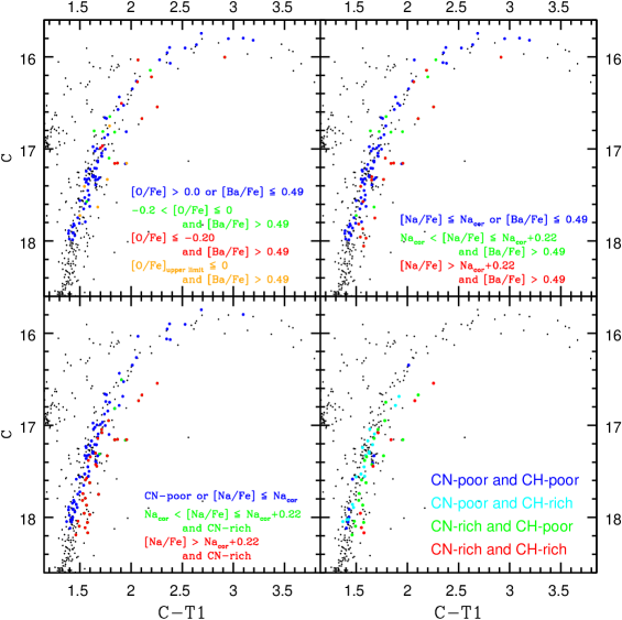
Figure 7.— In these four panels we look at various methods to distinctly differentiate the abundances of the red and blue RGB branches in the Washington filters. In the upper-left panel we see that considering O and Ba simultaneously has some success at differentiating the abundance characteristics of the two branches. This shows that the blue RGB are stars that are either O-rich or Ba-poor (blue), and the red RGB are stars that are both very O-poor and Ba-rich (red). In the upper-right panel we consider the more complete abundances of Na with Ba. This more clearly differentiates the blue RGB as stars that are either Na-poor or Ba-poor (blue), and the red RGB as stars that are both very Na-rich and Ba-poor. In the lower-left panel we consider CN-poor or Na-poor stars (blue), CN-rich and Na-rich (green), and CN-rich and very Na-rich (red). This most distinctly separates the two photometric branches. Lastly, in the lower-right panel we consider CN together with CH, where CH by itself did not show any meaningful photometric differences. Consistent with this, for CN-poor stars there is no significant difference between CH-rich and CH-poor stars. However, this comparison finds that the CN-rich stars that are consistent with the blue branch are primarily CH-poor and the reddest giants are both CN-rich and CH-rich.

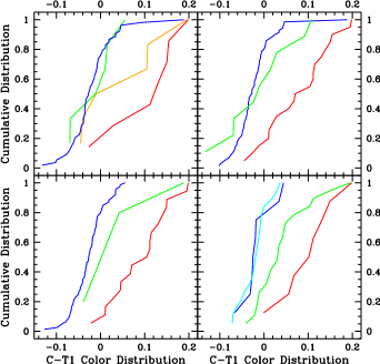
Figure 8.— We analyze the statistical properties of the photometric abundance distributions in Figure 7. Adopting the same abundance groups (and color schemes) we look at how the cumulative distributions compare between the defined abundance populations in C-T1 color space, adopting the same mean RGB trend as in Figure 4.

Another key element for differentiating the two populations is Ba. The Ba absorption itself is not significant enough to affect the observed flux, but its differentiating power may be related to a connection between Ba and N, where V10 found that the Ba-rich stars were also more N-rich. This is also found by our matching of the [Ba/Fe] from the much larger RGB sample in Ca11 to their CN abundances from Ca14; the Ba-rich stars are typically found to be more CN-rich by $\sim$0.15 dex. However, there is significant dispersion in the comparison and only evidence for a weak but statistically significant ($>$95% confidence) [Ba/Fe] and CN correlation. Whatever connection Ba may have, looking at the upper-left panel in Figure 3 shows that the Ba-poor stars show little scatter and almost all of them fall directly on the blue RGB, while the Ba-rich stars stars show a very large scatter covering both the red and the blue RGB.

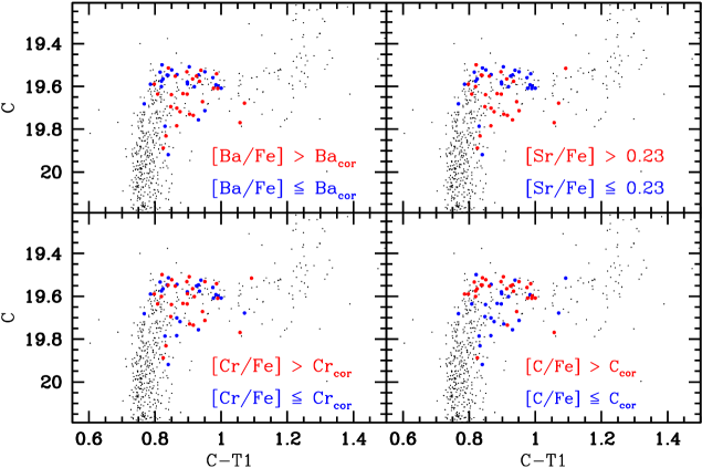
Figure 9.— Similar to Figures 3, 5, and 7, we now match SGB abundances from G12 to our Washington photometry of NGC 1851. In the upper-left panel we see that again, like in the RGB, Ba-poor (blue) stars nearly all fall tightly along the brighter (bluer) SGB while the Ba-rich (red) stars are more broadly distributed in color and create the sparser fainter (redder) SGB but still also fall on the bright SGB. Sr also creates a similar distribution. Cr, however, does not create a clear distinction between the two SGB branches. In the lower-right panel we look at the C abundances and show that the C-rich stars predominantly fall along the bright SGB while the C-poor stars are more broadly distributed. (See Figure 1 for the definitions of Ba_cor, Cr_cor, and C_cor.)

In Figure 7 we look at four approaches to distinctly characterizing the abundances of the red and blue RGBs. The upper-left panel simultaneously looks at both [O/Fe] and [Ba/Fe]. We have colored all of the Ba-poor (N-normal) stars blue and all of the O-rich stars blue because as discussed these stars should be CN-poor and either CH-poor or NH-poor. We clarify that these blue stars are either Ba-poor or O-rich and not necessarily both, and we include Ba-poor stars that do not have an O abundance and vice-versa. We have used three colors to mark the stars that are both Ba-rich and O-poor: green represents the Ba-rich and moderately O-poor stars, red represents the Ba-rich and very O-poor stars, and orange represents the Ba-rich stars with O upper limits that define them to be at least moderately O-poor if not very O-poor. Quite remarkably, the blue data are in agreement with the well defined blue RGB, while the green data show a moderately redder distribution typically falling on the red edge of the blue RGB and extending slightly redder, and the red data are mostly consistent with the red RGB. As should be expected the orange data are consistent with both the green and red data. This is promising but the matches are not perfect because two of the stars that clearly belong to the red RGB are colored blue. We also note the one colored red data point that lies well above the RGB. Its characteristics strongly suggest that it is an asymptotic giant branch star. This, rather than its abundances, explains its photometric deviation above the RGB. In the upper-left panel of Figure 8 we show the cumulative population distributions of these four abundance groups.

The one limitation of the Ca11 O abundances is that O is a challenging measurement. This resulted in 52 of the 111 stars we have matched to our photometry having only an upper limit or no O abundance information at all. Therefore, because Na has a well established anti-correlation with O and Ca11 has 108 measured Na abundances, we have analyzed a similar combination of Na and Ba abundances. This is shown in the upper-right panel of Figure 7 with all of the Ba-poor or Na-poor stars colored blue. The Ba-rich and Na-rich stars are grouped into Ba-rich and moderately Na-rich as green or Ba-rich and very Na-rich as red. This provides the most striking plot we have seen so far, where the blue data are consistently in agreement with the well defined blue RGB, while the green data show a moderately redder distribution typically falling where the red and blue RGBs meet, and the red data are consistent with the red RGB. Similarly, in the upper-right panel of Figure 8 we show the cumulative population distributions of these three abundance groups. Unlike with O, use of Na provides both a larger sample and abundance information extending to the faintest observed red RGB stars, where we still see abundance patterns consistent with the bright RGB stars. Overall, we have greatly increased the number of stars and find a result consistent with the proposed model.

As with Ba, the O (Na) abundances in combination with CN may tell us more. Again, the O abundances are limited in number, but the Na abundances will reliably be indicative of O. The lower-left panel of Figure 7 shows the combination of the CN strengths and Na abundances, where we color stars that are both CN-rich and very Na-rich (very O-poor) red, the CN-rich and moderately Na-rich stars green, and all stars that are either CN-poor stars or Na-poor blue. We now see that when considering the O abundances (represented by Na) in addition to the CN strengths, the red data and the blue data agree very well with the red RGB and the blue RGB, respectively, and the green data primarily falls where the red and the blue RGB meet. This is displayed more clearly in the lower-left panel of Figure 8, where there is almost no color overlap between the red and blue population distributions. This result implies that because of the possible lack of large C+N+O variations, the CN-rich and Na-poor (O-rich) stars will not be both very C-rich and N-rich, so their moderately strong CN strengths will be balanced out by either weak CH or NH lines. Additionally, the CN-poor and Na-rich stars are O-poor but likely have band strengths limited by weak N or weak C. Only the CN-rich and the Na-rich (O-poor) stars will be significantly rich enough in both C and N to also be CH-rich and NH-rich, leading only these stars to be significantly fainter in the C magnitude.

Lastly, in the lower-right panels of Figures 7 and 8 we consider CH and CN band strengths together. Here stars that are both CN-poor and CH-poor are blue, those that are both CN-poor but CH-rich are cyan, those that are both CN-rich and CH-poor are magenta, and lastly those that are both CN-rich and CH-rich are red. Remarkably consistent with our explanation given at the beginning of this section, and most clearly shown in the lower-right panel of Figure 8, for the CN-poor stars the variations in CH strengths (i.e., [C/Fe]) have no meaningful affect on the resulting color. This is not the case for the CN-rich stars, where all CN-rich stars consistent with the blue RGB are also CH-poor, while the red RGB is composed of nearly all of the stars that are both CN-rich and CH-rich.

4. Matching Turnoff/Subgiant Branch Abundances to Photometry

We have also matched the SGB and turnoff abundances of G12 to our photometry. While the lack of [O/Fe] and [Na/Fe] measurements for these stars limit us from performing the more detailed analysis we did with the RGB stars, we still detect that in several elements the two branches exhibit different abundance characteristics. In Figure 9 both [Ba/Fe] and [Sr/Fe] show similar patterns as those observed for Ba in the RGB. The Sr-poor stars and Ba-poor stars are both concentrated on the brighter and blue branch while the Sr-rich stars and the Ba-rich stars are more broadly distributed and create the sparse fainter and red branch but also compose part of the bright branch. Sr and Ba are the two elements that both G12 (in the SGB) and V10 (in the RGB) show to be strongly correlated. The Cr-rich and Cr-poor stars do not show a strong photometric distinction; this illustrates the importance of adopting the observed trends (see Figure 1) to define rich and poor populations because adopting a constant separation for Cr-rich and Cr-poor does result in an apparent photometric distinction in the SGB. These Ba and Sr distributions suggest that in the C filter, as on the RGB, these are not two photometrically distinct SGB sequences representing two cleanly separated populations, but that photometrically the two populations are a narrow and a broad population that overlap each other. The broad second population extends significantly farther to the red and creates a distinctly redder branch, but again this clearly redder group is not the entire second population.

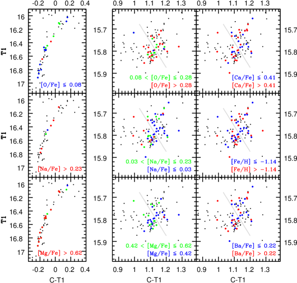
Figure 10.— Matches of the HB abundances from G12b to our Washington photometry of NGC 1851. The left grid of three panels shows the BHB and the right grid of 6 panels shows the RHB, with its two potential sequences: a faint (bluer) sequence and a bright (redder) sequence, which we have divided by a solid grey line. O, Na, and Mg have both BHB and RHB abundances and their abundances distributions are very broad. Therefore, we have grouped them in three abundance groups with blue being poor, green being intermediate, and red being rich. This clearly illustrates the abundance distinctions between the RHB and BHB. Looking closely at the RHB itself finds that there are no clear abundance distinctions between the two apparent RHB sequences in any of these six elements.

G12 also have direct measurement of the C abundances from the CH bands for the SGB stars, which we discussed a temperature trend for in Section 2 and Figure 1. Using the correlation from Figure 1 to define our C-rich and C-poor populations and matching these abundances to our photometry shows that the faint SGB is predominantly C-poor while the bright SGB is predominantly C-rich. This is in contrast to what we would infer based on the RGB abundances and CH indices, but the bright SGB is on average only $\sim$0.1 dex richer in C. This difference is relatively minor compared to the total range of C abundances, when correcting for the trend with T_eff, spanning $\sim$0.6 dex. To expand on this further, we can define the two SGB populations based on their [Ba/Fe], and we find that the Ba-rich (second population) and Ba-poor (first population) stars have on average no meaningful difference in C.

We also acknowledge the work in L12, which self-consistently added to the work of Pancinco et al. (2010) and in total analyzed 70 turnoff and SGB stars. They found C and N abundances from their direct measurement of the CH and CN bands and matched them to both the HST photometry of Milone et al. (2008) and the Stromgren photometry of L09. They similarly found that the bright (blue) SGB is typically more C-rich and the faint (red) SGB is typically more C-poor, but also that the bright SGB is poorer in N and the faint SGB is richer in N. They argue that there is a significant and possibly bimodal spread in the distribution of C+N abundances, with the faint SGB typically being much richer.

Figure 11.— Illustration of the bimodal RHB distribution perpendicular to the solid grey dividing line shown in Figure 10.

G12 question these large variations in the L12 C+N abundances and suggest that their T_eff were 500 K too cool. This would cause them to greatly underestimate the C abundances, and because the N abundances are found from CN this would also cause the N abundances to be overestimated. However, based on the idea that C+N+O is fairly constant, this variation in C+N would at least be qualitatively in agreement with the variations in O abundance observed in the RGB. The C+N-rich stars would be O-poor and the C+N-poor stars would be O-rich. L12 also concluded this by comparing the average RGB O-abundances from V10 to their average C+N abundance for the two branches and found no meaningful difference between their average C+N+O abundances. We have also matched 65 of the abundances from L12 to our photometry, but only one of these stars could reasonably be defined as belonging to our faint SGB. Most of the limited number of faint-SGB stars from L12 were affected by crowding issues in our ground-based photometry from Paper I. The one clear faint-SGB star from Paper I with L12 abundances is both N-rich and C-rich, but this is too limited to draw any conclusions.

5. Matching Horizontal Branch Abundances to Photometry

The horizontal branch (HB) abundances provide a unique case to analyze the two populations because here they create two photometrically distinct groups of stars in the blue and red HB, unlike the overlapping RGBs and SGBs. It is believed that the BHB corresponds to the red and broader population on the RGB and that the RHB corresponds to the blue and narrower population on the RGB. The distinct color differences in the HB itself are believed to result from a moderate He enhancement in the BHB population (e.g., the observations of G12b and the models of Joo & Lee 2013). This variation in He can also explain the observed variations of the pulsational properties of RR Lyrae variables in NGC 1851 (Kunder et al. 2013). Another advantage of the HB is that these are bright stars with relatively small photometric error. Our observations from Paper I were able to observe a broad range of both T1 and T2 magnitudes in the RHB, and in T1 there is an apparent split that creates two sequences of T1 magnitudes. Does this suggest that there may be key differences for stars within the RHB itself?

Figure 10 shows the abundances from G12b matched to the RHB and BHB (when available). Similar to previous Figures for Ca, Fe, and Ba the blue data represent poor stars and the red data represent rich stars for each element. However, for the elements that also have BHB abundances measured we used three abundance groups because they typically have very broad elemental distributions: for O the red data represent O-rich stars, the green data represent moderately O-poor stars, and the blue data represent very O-poor stars. For Na and Mg the blue data represent poor stars, the green data represent moderately rich stars, and the red data represent very rich stars (see Figure 10 for the detailed abundance ranges).

The BHB is very O-poor, Na-rich, and very Mg-rich, consistent with it being the same population that creates the red RGB. The RHB overall does show a broader range of O, Na, and Mg abundances than the BHB, but there are no consistent abundance differences between the two apparent RHB sequences. While the faint RHB may on average be more O-poor, Na-rich, and Mg-rich, it still contains many O-rich, Na-poor, and Mg-poor stars. For both [Fe/H] and [Ca/Fe] there are no meaningful abundance differences between the two RHB sequences, but when considering errors the observed distribution spreads in [Fe/H] and possibly [Ca/Fe] are not meaningful. Lastly, Ba appears to similarly show no meaningful difference between the bright and faint RHB, but there is a meaningful sample of very Ba-rich stars ([Ba/Fe]$>$0.5; see Figure 2) that nearly all fall on the faint RHB.

To look more closely at the double distribution in NGC 1851, we divide the two sequences with the solid grey line shown in Figure 10 (T1=14.487+(C-T1)$\times$1.156). In Figure 11 we illustrate the bimodal distribution perpendicular to this dividing line. This also provides a reference to statistically test for differences in photometric distributions on the RHB abundances of Figure 10. Consistent with expectations, there are no significant (p-value $<$ 0.05) differences in distribution of any of the defined abundance groups within the RHB. Even the very-rich Na stars in Figure 10 ([Na/Fe]$>$0.23), which in the RHB primarily fall on the faint RHB, do not have a statistically meaningful difference in distribution in comparison to the Na-poorer ([Na/Fe]$\leq$0.23) stars. This is because while a KS-test provides a moderate D of 0.4312, the small number limitations of only 11 very-rich Na RHB stars gives a p-value of only 0.063. However, we again make note of the RHB stars richest in Ba ([Ba/Fe]$>$0.5) all primarily fall on the faint RHB. They have a meaningfully different photometric distribution in comparison to all RHB stars with weaker Ba, where a KS-test test provides a D of 0.4701 and a p-value of 0.033.

In comparisons to other cluster, this double sequence in the RHB of NGC 1851 appears similar to the double sequence in the RHB of 47 Tuc (Milone et al. 2012). But unlike NGC 1851, 47 Tuc does not also have a BHB. Another distinction is that these two 47 Tuc RHB sequences are separated in the UV. Therefore, adopting in 47 Tuc two populations with appropriate CNO variations that can create its observed double sequences in the MS, SGB, and RGB would also create this double sequence in the RHB. In NGC 1851 its two populations instead create its well observed BHB and RHB. Is this the result of the NGC 1851 populations possibly having a more significant difference in He than those of 47 Tuc? The two RHBs of NGC 1851 are further differentiated because they are not defined by a difference in UV but by differences in the T1 and T2 magnitudes, which are not meaningfully affected by variations in CNO.

Is there a possible age spread between these two RHBs? Milone et al. (2008) suggested an age difference of $\sim$1 Gyr between the two NGC 1851 populations to explain the observed split SGB, but this corresponds to the RHB and the BHB. Is there possibly a spread in age between the apparently single population that creates the RHB? Is there some factor driving a difference in mass-loss rates between the two RHB sequences? Lastly, is this related to the four, not just two, abundance group spectroscopically observed in NGC 1851 by Campbell et al. (2012) and Simpson et al. (2017)?

The apparent double RHB remains a mystery, but the differences between the RHB and BHB have further established the key abundance differences between the two populations of NGC 1851.

6. Photometric Synthesis of Red Giant Branch Populations

To create our synthetic magnitudes we applied the models of Kurucz et al. (1992) with overshoot and used the spectral synthesis program SPECTRUM v2.76⁴ and its linelist (Gray & Corbally 1994). For our standard input abundances we applied a [Fe/H] of -1.23, which is based on that found by V10 (-1.23$\pm$0.01) and is similar to that found by Ca11 ([Fe/H]=-1.16$\pm$0.05). We also applied a standard He abundance of Y=0.246. To analyze the effects of possible variations in He, we have performed comparisons to a more He-rich (Y=0.30) population. For CNO abundances we applied the result of V10 that for both populations C+N+O is constant at log $\epsilon$(CNO)=8.00. Additionally, we considered the effects of distinct log $\epsilon$(CNO) in the two populations that results from the more significant differences in [N/Fe] measured in Y15. This gives the second population a significantly richer log $\epsilon$(CNO)=8.50. All other abundances are scaled solar.

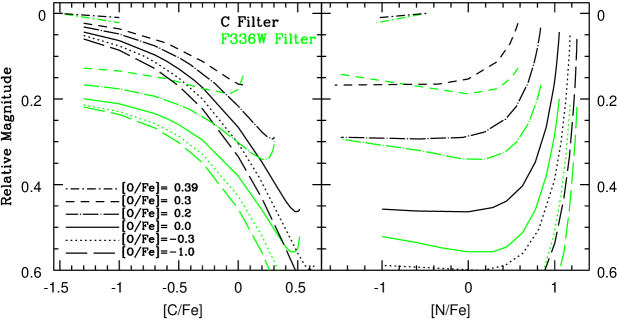
Figure 12.— Relative magnitude synthesis of a representative RGB star for the Washington C filter (black) and the F336W filter (green). Varying levels of [C/Fe], [N/Fe], and [O/Fe] are considered but with an adopted constant log $\epsilon$(CNO)=8.0. The different curves represent constant [O/Fe] (see key) with corresponding variations in [C/Fe] (illustrated in the left panel) and [N/Fe] (illustrated in the right panel). Both panels show reflections of the same data curves in [C/Fe] and [N/Fe] space, respectively. For both filters their magnitude at the most C-poor abundance synthesized is defined as the zero point (brightest) and as standard an increase in magnitude (going down the y-axis) is increasingly fainter. This demonstrates the strong dependence of C magnitudes on [C/Fe] across a large range of abundances. F336W magnitudes are also strongly dependent on [C/Fe] but are more counterbalanced by an important dependence on [N/Fe].

Variations in [Fe/H] can also play an important role in MPs, but evidence for a meaningful spread in [Fe/H] in NGC 1851 is limited to the analysis in the RGB by Ca11. V10 did not find any evidence for such a spread. If there is a true variation it is relatively minor ($\sim$0.1 dex). Additionally, matches of these [Fe/H] values to both Stromgren photometry (see Ca11) and our own Washington photometry find that these apparent [Fe/H] variations do not match with the two identified populations and are randomly distributed photometrically. Therefore, if this minor [Fe/H] variation is real it does not play a role in the photometric differences of the two populations, and it would only increase the photometric spread observed in each population. For completeness, however, we briefly considered the photometric effects of a 0.1 dex metallicity increase.

6.1. Effects of CNO on Magnitude at Constant Log $\epsilon$(CNO)

To thoroughly evaluate the effects of variations of C, N, and O, we analyzed nearly the full range of abundances within the constraint of log $\epsilon$(CNO)=8.0. This allows us to move beyond the constraints of the abundances of NGC 1851 and also make more general conclusions about the photometric effects of CNO variations at constant log $\epsilon$(CNO) and how this varies in differing filters.

For our representative RGB star we adopted T_eff=4863 K, log g=2.18, microturbulence=1.52 km/s, and [Fe/H]=-1.23. This places this giant right below the RGB bump in NGC 1851. In addition to the C filter we also synthetically looked at the commonly adopted F336W filter (which is very similar to Johnson U). In contrast to both the C and Stromgren filters, Johnson U appears to create two more cleanly separated photometric branches in the RGB of NGC 1851 (H09) instead of heavily overlapping narrow and broad branches. However, based on published analyses of NGC 1851, it is unclear if the U or F336W filters also distinctly separate, for example, the Ba- and Na-poor stars from the Ba- and Na-rich stars. H09 showed that in U-I their red branch is Ca-rich and their blue branch is Ca-poor with little meaningful overlap, but these Ca abundances were photometrically based, and Han et al. subsequently discovered that their Ca filter was old and degraded, leading to an increased sensitivity to CN variations and a decreased sensitivity to Ca variations. In other clusters, however, the recent photometric and spectroscopic analysis of the similar double RGB in M2 (Lardo et al. 2013) also finds in U-V that the redder RGB is cleanly separated from the bluer RGB. The abundance and spectral indices in Lardo et al. (2013) also illustrate that U magnitudes cleanly separate stars of differing Sr and Ba abundances and CH and CN indices. These characteristic differences in how MPs are photometrically distributed in C and U or F336W filters was briefly discussed in Paper I, but in this Section and the following we will analyze the reasons for this difference in more detail.

The general relations between abundance and magnitude for the C and F336W filters can be defined by looking at broad abundance ranges for [C/Fe], [N/Fe], and [O/Fe]. Figure 12 assumes a constant log $\epsilon$(CNO)=8.00, and the left panel looks at several curves of constant [O/Fe] and how variations in [C/Fe] affect both C magnitudes and F336W magnitudes. We remind the reader that variations in [C/Fe] must have corresponding [N/Fe] variations in order to keep total CNO constant, which are similarly illustrated in the right panel of Figure 12. Throughout this paper we focus on the comparisons plotted relative to [C/Fe] because the general characteristics are more clearly displayed in this manner. The magnitudes are placed on a relative scale where the magnitude of the most C-poor and O-rich abundance we analyzed ([N/Fe]=-0.49, [C/Fe]=-1.50, and [O/Fe]=0.39) is set as the zero-point for both filters. Each curve represents a constant [O/Fe] with black curves for the C filter and green curves for the F336W filter. Lastly, we find that these same very broad variations in CNO have only marginal effect on the synthetic R (T1) magnitudes ($\lesssim$0.02 mag, or only 2 to 5%  of the variations found in C magnitude) but they become more important for the synthetic I (F814W) magnitudes ($\lesssim$0.04 mag, or 4 to 10%  of the variations found in C magnitude or 2 to 7%  of the variations found in F336W). Therefore, these plotted variations in C and F336W magnitude reliably trace variations in C-T1 and F336W-F814W, in particular when looking at realistic (moderate) CNO variations observed within a single cluster, but for the highest precision comparisons to cluster observations these variations in R (T1) and I (F814W) should be noted.

At constant [O/Fe], increasing [C/Fe] with the corresponding decrease in [N/Fe] leads to a fainter C magnitude in all but the richest [C/Fe] (weakest [N/Fe]). Therefore, in the C magnitude the [C/Fe] generally plays the dominant role, which was the filter’s original purpose (note that the C designation in fact refers to Carbon). [N/Fe] remains important but generally plays a secondary role. In contrast, the F336W magnitude patterns are more complex and typically show at constant [O/Fe] a relatively weaker dependence of F336W magnitude on [C/Fe], but followed by quickly brightening F336W magnitude at the richest [C/Fe]. This pattern can be explained by the F336W filter being strongly dependent on [C/Fe] but [N/Fe] plays nearly as important of a role, resulting from the prominent NH band at 3360 Å  near the center of its bandpass and the lack of the CH feature at 4300 Å (the G band). In contrast the G band plays a more important role in the C filter while the strong NH band is at the far blue edge of its bandpass where the transmission is relatively low. Therefore, for the F336W filter in Figure 12 the increasing [C/Fe] at constant [O/Fe] is counterbalanced by a decreasing [N/Fe], leading to a comparatively weaker magnitude change with increasing [C/Fe] followed by a significant brightening at the C-rich extreme because so little N remains, greatly weakening the NH line.

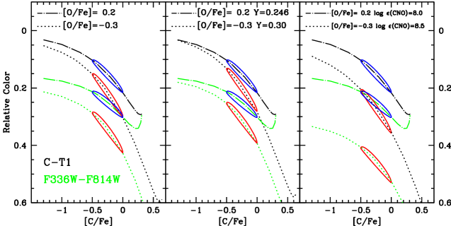
Figure 13.— The left panel applies the curves from Figure 12 to C-T1 and F336W-F814W color space for abundances of the two populations in NGC 1851. An O-rich/N-normal population is circled in blue and an O-poor/N-rich population is circled in red for both color curves. This illustrates photometric variations similar to the corresponding observations of Paper I for C-T1 (a narrow blue population and a heavily overlapping but broad red population) and H09 for U-I (which is comparable to F336W-F814W with two more cleanly separated populations). The central panel looks at identical CNO variations but illustrates the effects of O-poor/N-rich population ([O/Fe]=-0.3) also being He-rich (Y=0.30). This causes this redder population to be shifted slightly bluer, but the two populations are still distinct. The right panel looks at the significant effect of the O-poor/N-rich population ([O/Fe]=-0.3) also having a richer log $\epsilon$(CNO)=8.5. The significant increase in [N/Fe] shifts the redder populations $\sim$0.06 further to the red in C-T1 and $\sim$0.12 further to the red in F336W-F814W.

Comparing the relative shifts in the differing lines (representing changing [O/Fe]) indicates another key difference between the two filters caused by the stronger [N/Fe] dependence of F336W. With increasing [O/Fe], at constant [C/Fe], the F336W magnitudes become fainter more rapidly than the corresponding C magnitudes. This is not directly the result of the changing [O/Fe], which plays relatively little importance in the actual flux, but the corresponding increase in [N/Fe] with the decreasing [O/Fe]. This also represents the advantage that the F336W (and the similar Johnson U) filter has over the C filter in separating MPs that have a significant difference in [N/Fe]. It is also important to note an anti-correlation (or correlation) between NH and CH strengths is not clearly observed in NGC 1851, but they are observed in most globular clusters (e.g., Pancino et al. 2010; L15). For clusters with anti-correlations (e.g., 47 Tuc, M15, NGC 288) the weaker CH bands in the N-rich/O-poor second population will weaken the observed magnitude shift in C more than it does in F336W, but for clusters with a positive correlation (e.g., M22) this will increase the C magnitude sensitivity more than for F336W. Despite these caveats, the C filter is still highly sensitive to CNO abundance variations and retains many advantages with its significant (4 to 5 times) increase in photometric throughput in cool RGB stars versus the F336W filter.

6.2. Application to NGC 1851 Red Giant Branch Abundances

Here we apply these curves more specifically to the photometric and spectroscopic observations of NGC 1851. In Figure 13, because we look at a number of special cases where variations in R (T1) and I (F814W) play a role, we plot these curves in color space with C-T1 in black and F336W-F814W in green. In the left panel of Figure 13 we have selected two appropriate abundance ranges for the two observed populations of NGC 1851. Both populations have a comparable average [C/Fe] of $\sim$-0.25 but with a moderate variation, consistent with no CN-CH correlation. The dominant blue population has a [O/Fe]$\sim$0.2 while the secondary red population has a [O/Fe]$\sim$-0.3. This is more C-rich than the RGB abundances measured by V10 and Y15, but those are from upper RGB stars where deep mixing has further depleted the [C/Fe] beyond the lower RGB and the SGB. For both the C-T1 and F336W-F814W curves we illustrate the abundance groups with a blue and red ellipse plotted over each curve set. As would be expected, the O-rich/N-normal population (blue ellipse) has both brighter C and F336W magnitudes giving relatively narrow and blue populations in both colors. Also, as expected, the O-poor/N-rich population (red ellipse) has both fainter C and F336W magnitudes, giving redder colors, but there are many key differences. First, in C-T1 the weaker [N/Fe] sensitivity leads to a relatively weaker color difference causing strong overlap between the primary and secondary population at the O-poor/C-poor edge versus the O-rich/C-rich edge. However, the sensitivity of C-T1 to varying [C/Fe] is increased in the O-poor stars giving a very broadly distributed color range with a distinctly redder subpopulation consisting of only the O-poor/N-rich/C-rich stars. The second population (O-poor/N-rich) in F336W-F814W shows more significant color separation from the primary blue population. Additionally, the weaker sensitivity to [C/Fe] variations leads to a narrower population than observed in C-T1. These findings are strongly consistent with our observations in Paper I of the two RGB branches in C-T1 and C-T2 and the comparable U-I used by H09.

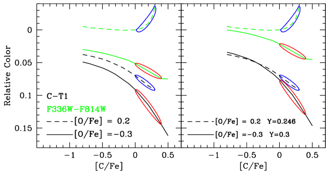
Figure 14.— The left panel shows the relative color synthesis of a representative upper MS star for C-T1 (black) and for F336W-F814W filter (green). The format is the same as that described in Figure 13. Additionally, the C-T1 and F336W-F814W curve sets are arbitrarily offset for clarity. While the [C/Fe] sensitivity of these colors are weaker here than in the RGB, due to the hotter T_eff, it is still strong and the trends are similar to that found in the RGB. We note that in the MS these same two populations should overall be more C-rich and correspondingly poorer in N than the RGB. Two photometrically separated populations are predicted in both colors. A double MS, however, has not been observed in F336W-F814W for NGC 1851. In the right panel we consider that the redder (O-poor/N-rich) population is likely also He-rich. Adjusting the relative colors for an He difference greatly diminishes the predicted photometric difference in F336W-F814W, and with only moderate photometric error these populations may appear as a somewhat broad but single MS. The C-T1 color difference is also diminished, but the O-poor/N-rich population remains significantly broader in color and can be detected more easily through the distribution analysis performed in Paper I.

The consistency of the general photometric characteristics seen in observations is promising. More quantitatively, the observations in both Paper I and H09 find an observed difference of $\sim$0.1 in C-T1 and U-I colors, respectively, between the centers of the two RGB branches. This is consistent with the separation of the centers of the red and blue ellipses in F336W-F814W color. For C, while the separation of the two ellipses in C-T1 color is $\sim$0.05, this is the separation of the two complete and overlapping populations. The RGB “red branch” in C-T1 is only the redder half of the red ellipse, and again it has an extension of $\sim$0.1 beyond the dominant blue branch. (For reference, the O-poor/N-rich population is only $\sim$0.005 magnitudes fainter in R (T1) and $\sim$0.015 magnitudes fainter in I (F814W; T2) in comparison to the O-rich/N-poor population. The lack of significant effect of CNO variations on these redder filters is also consistent with the two RGB branches not being observed in Paper I’s T1-T2.)

While our photometric matches do not find that redder RGB population is more metal-rich, it is important to test what effects metallicity variations may have between the two populations. Adopting that the O-poor/N-rich population is also 0.1 dex richer in all metals (besides CNO) finds that all filters are moderately affected. Accounting for the effects in both filters, the metallicity increase would shift the O-poor/N-rich population $\sim$0.02 redder in C-T1 and $\sim$0.025 redder in F336W-F814W. By itself, this metallicity increase is not large enough to create the observed color differences between the two populations in NGC 1851, but this shows that metallicity is important to consider in clusters with well defined metallicity differences between their MPs. As suggested by the NGC 1851 observations in Ca11, however, if there is a true metallicity spread of $\sim$0.1 dex within each population, this would further enhance the color spread within each population.

In the center panel of Figure 13 we also consider the effects of the second population (O-poor/N-rich) being more He-rich (Y=0.3) than the first population. In an RGB star of these characteristics, this has minor but measurable effects on its F336W and C magnitudes. However, we note that variations in He also have smaller but meaningful effects on the R (T1) and F814W (I) magnitudes. Therefore, in the center panel of Figure 13 we account for all filter variations in our color curves. As expected, a richer He shifts the both C-T1 and F336W-F814W to bluer colors.

In the right panel of Figure 13 we look at the effects that an increase of log $\epsilon$(CNO) from 8.0 to 8.5 for the second population would have. This is driven by a significant increase in [N/Fe] but with consistent [O/Fe] and [C/Fe] abundances and is in line with with the abundances from Y15. Unlike at constant log $\epsilon$(CNO), this variation in total log $\epsilon$(CNO) leads to more important effects on R (T1) at $\sim$0.03 and F814W (I) at $\sim$0.05. Therefore, we apply the effects of all filters on our colors. We find that this large increase in [N/Fe] causes a significant shift to the red for the second population that is far more than is found in either C-T1 or U-I observations. Even when correcting for the second population also being richer in He, this remains inconsistent with observations. One additional factor suggested by the abundances of V10 and G12 is that the second population on average is slightly ($\sim$0.1 dex) more C-poor. This would help mitigate the effect of such a large increase in [N/Fe] and suggests that the log $\epsilon$(CNO) may not be uniform across both populations, but any differences are likely more moderate ($\lesssim$0.2-0.3 dex).

7. Photometric Synthesis of Main Sequence Populations

In Paper I, using Washington photometry we discovered evidence for NGC 1851 having two photometric branches in the MS consistent with those observed in its RGB. Unlike in the other stellar groups, there are no direct spectroscopic abundances available for MS stars in NGC 1851. However, we can still infer general abundance information from the observed SGB and RGB abundances. Therefore, we have looked specifically at an O-rich ([O/Fe]=+0.2) population and an O-poor ([O/Fe]=-0.3) population, consistent with our RGB analysis and the abundances of Ca11. At these [O/Fe] we again adopt a constant log $\epsilon$(CNO)=8.0 and at a range of [C/Fe] near scaled solar. Our representative MS model has T_eff=5800 K, log g=4.59, microturbulence=0.74 km/s, and [Fe/H]=-1.23. This places our star in the upper MS below the turnoff.

Figure 14 looks at the color synthesis for an MS star in both the C and F336W filters. Both the general C-T1 and F336W-F814W color trends are consistent with that found in the RGB (Section 6). Again, these color variations are driven by magnitude variations in C and F336W because the synthetic R (T1) and F814W (I) magnitudes variations ($<$0.01) are even weaker than those predicted in the RGB. Overall, in comparison to the RGB, the variations in synthetic color are weaker but still significant. This is primarily the result of the MS model star being $\sim$1000 K hotter than the RGB model star, giving weaker CN, CH, and NH bands, rather than any other difference between MS and RGB stars.

Focusing on the expected abundance differences in the two MS populations of NGC 1851, the [C/Fe] abundances of the SGB and upper turnoff stars from G12 (see Figure 1) suggest that the [C/Fe] in the MS will have moderate variations and be richer than scaled solar. The MS is expected to be more C-rich than the RGB because the mixing processes that dilute the surface C during evolution have not yet begun. In Figure 14 we have adopted abundance ranges consistent with this for the two MS populations and find that the O-rich/N-normal population (blue ellipse) is bluer in both C-T1 and F336W-F814W and relatively narrow, but at these very C-rich abundances the decreasing [N/Fe] makes the F336W-F814W colors increasingly bluer. The O-poor/N-rich population (red ellipses) create in C-T1 a very broadly distributed and slightly redder population with minor overlap with the blue population. The F336W-F814W creates a significantly redder but still photometrically narrow population.

Milone et al. (2008) did not find evidence in NGC 1851 for a double MS in F336W-F814W, but the C-T1 observations from Paper I do find evidence for a heavily overlapping but broadly distributed second redder MS. In the upper MS this second MS extends to the red with an apparent separation of $\sim$0.05 magnitudes. In the lower MS this separation increases further, resulting from the increasing strengths of the molecular bands in cooler stars.

Figure 14 suggests that the double MS should be cleanly separated in the F336W-F814W observations of Milone et al. (2008), but this is not the case. A possible explanation for this is that in the MS the effect of the varying He abundances in the two populations becomes more important. The O-poor/N-rich population is believed to be more He-rich. In the right panel of Figure 14 we analyze the effects of this by keeping the O-rich/N-normal population at our standard Y=0.246 and the O-poor/N-rich population at Y=0.30. Across the range of [C/Fe] and [N/Fe] at constant [O/Fe]=-0.3, the effect on the C and F336W magnitudes are uniform at 0.043 brighter and 0.052 brighter, respectively. The He-rich population is also 0.028 magnitudes brighter in T1 and 0.022 magnitudes brighter in F814W. This shifts the He-rich population 0.03 magnitudes bluer in F336W-F814W and 0.015 magnitudes bluer in C-T1. This brings the populations in C-T1 closer together but because of their distinct color distributions the heavily blended redder population was still observed in Paper I using C-T1. However, the larger effect of He on the F336W-F814W color nearly brings the two narrow MS populations together. With even small photometric error and considering that this second population may be slightly more C-poor ($\sim$0.1 dex), this may appear similar to a single MS that is broad in color but otherwise normal.

8. Summary & Conclusions

Matching previously published spectroscopic abundances to our Washington photometry, we have analyzed many of the quantitative differences between the two NGC 1851 populations. The large sample of RGB abundances from Ca11 have shown that Ba, Na, and O are useful elements to distinguish between the two populations in the RGB. In particular, Ba and Na clearly show that stars poor in either of these elements are consistently part of the (in C-T1) narrow and blue RGB, while stars that are rich in either of these elements are more broadly distributed in color. The reddest stars of this second population create the red RGB while the bluer stars of this second population are consistent in color with the blue RGB. In agreement with the strong O and Na anti-correlation, the O-rich stars are consistent with the narrow and blue RGB while the O-poor stars are more broadly distributed. To better understand this broad color distribution of the second population, we considered two abundances simultaneously. The stars that are both Ba-rich and O-poor (or similarly Ba-rich and Na-rich) all fall primarily on the red RGB. All other stars are consistent with the blue RGB. This may result from [Ba/Fe] acting as a tracer of [N/Fe]. Therefore, the red RGB is composed of only the N-rich/O-poor stars. This is further supported because stars that are both CN-rich and Na-rich (or CH-rich) all fall primarily on the red RGB.

Matching the G12 abundances to the two branches of the SGB shows many consistencies with what we found in the RGB abundances, in particular for the correlated elements of Ba and Sr. While the lack of O and Na abundances for the SGB limit our analysis tools, the C abundances from G12 are useful to analyze these two branches. Most interestingly, the C abundances from G12 suggest that the faint SGB is more C-poor and the bright SGB is more C-rich, but the difference is only $\sim$0.1 dex while the total range of C abundances span $\sim$0.6 dex.

For the G12b abundances of the HB, as expected we find clear abundance differences between the RHB and BHB where the BHB is relatively very O-poor and more Na-rich and Mg-rich. However, other than a group of very Ba-rich stars being predominantly in the faint RHB, there are no clear abundance differences between the observed bright and faint RHB sequences. The cause of these sequences in the T1 and T2 magnitudes remains unclear, but it is likely different than the CNO and He variations that can explain the two established populations, represented by the BHB and the RHB. It would be of interest to investigate what other factors may cause two sequences of such characteristics in the “single population” of the RHB.

To build on these abundance analyses and look at the role that CNO plays in the C and F336W filters, we performed photometric synthesis for a broad range of [C/Fe], [N/Fe], and [O/Fe] at a constant log $\epsilon$(CNO)=8.0. Comparisons of the effects on both the C and F336W filters find that at constant C+N+O the variations in magnitude can be quite significant and adopting larger log $\epsilon$(CNO) values are not necessary to explain the observed photometric differences between the two populations. This analysis also showed that the C filter is highly sensitive to [C/Fe], as its name would suggest, with some sensitivity to [N/Fe]. In contrast, F336W and the similar Johnson U filter have more comparable sensitivities to both [C/Fe] and [N/Fe].

To compare these synthetic magnitudes to observations of NGC 1851, we adopted abundance characteristics for each population based on the RGB spectral analyses from Ca11, V10, Ca14, and Y15. We define the two populations as an O-rich ([O/Fe]=0.2) and an O-poor ([O/Fe]=-0.3) population. In our representative RGB star that is just below the RGB bump, we assume that both populations have comparable but broadly distributed [C/Fe] near [C/Fe]$\sim$-0.25, which is consistent with NGC 1851 not having a CN-CH correlation. Based on the constant C+N+O, and consistent with the CN observations of Ca14, the O-rich and O-poor populations are also N-normal and N-rich, respectively. Application of this to our photometric synthesis finds that the O-rich/N-normal population is blue and narrowly distributed in color in both C-T1 and F336W-F814W. Similarly, the O-poor/N-rich population are both redder in C-T1 and F336W-F814W. However, in C-T1 the second population’s colors are very broadly distributed and overlapping with the bluer population. In F336W-F814W the second population is redder and nearly as narrow in color as the blue population. These color variations are driven almost completely by variations in the C and F336W filters and are consistent with the photometric observations of both Paper I and H09.

In application to general globular cluster observations, it is important to discuss the differences between clusters with a CN-CH anti-correlation or correlation in contrast to our adoption of no correlation (as observed in NGC 1851). In general, the photometric sensitivity to MPs will be decreased in clusters with CN-CH anti-correlations, but more so in the C filter versus F336W. However, for clusters with CN-CH correlations the increase in photometric sensitivity to MPs will be greater in the C filter versus F336W. Our broad abundance analysis in Figure 12 helps illustrate this.

We also looked at additional differences that may play a role in the photometric differences of these two populations. First, we considered the O-poor/N-rich population being He-rich (Y=0.3). This diminishes the color difference between the two populations, but the effect is relatively minor and the predicted total photometric differences are still significant and detectable. Second, we considered the O-poor/N-rich population being significantly more N-rich than the primary population at log $\epsilon$(CNO)=8.5. This greatly increases the predicted color differences between the two populations, strikingly in F336W-F814W, and well beyond the differences that have been observed in NGC 1851. A more moderate difference in log $\epsilon$(CNO) ($\lesssim$0.2 to 0.3) for the two populations, however, could be further mitigated by the O-poor/N-rich population being both He-rich and slightly more C-poor ($\sim$0.1 dex). This could bring two populations of a meaningfully different log $\epsilon$(CNO) into agreement with the photometric observations.

Applying the same [O/Fe] based populations to photometric synthesis in the MS finds further interesting comparisons between the C and F336W filters. Because the MS will be more C-rich we adopted a moderately spread [C/Fe] consistent with that found in the least unevolved stars from G12 ([C/Fe]$\sim$0.2). In the hotter MS stars, compared to the cooler RGB stars, the weaker molecular bands lead to comparable dependencies but overall less significant sensitivity to the CNO abundances in both the C and F336W filters. At these richer [C/Fe] the second, redder population is still very broadly distributed in the C-T1 but quite narrow in F336W-F814W. This is consistent with the observations of a heavily overlapping double MS from Paper I, but how does it explain the lack of observed double MS in the F336W-F814W observations of Milone et al. (2008)? We believe this again relates to the increase in He abundance in the second O-poor/N-rich population. In the MS the increase in He has a more important effect than in the RGB, and it is also stronger in the F336W-F814W colors than the C-T1 colors. This He correction is significant enough that in F336W-F814W the two narrowly distributed in color MS populations are nearly shifted on top of each other. Considering appropriate photometric error and the second population being slightly more C-poor ($\sim$0.1 dex), this could create a broad but apparently single MS. In C-T1, the significant difference between the color distribution widths of the two populations leaves a comparably overlapping but more distinguishable second population.

The C filter is a very important filter in analyzing the MPs in GCs for four reasons. The first is that in the typically very cool stars in GCs the C filter has $\sim$3 to 5 times the throughput of other UV filters. This results from the C filter being both broader but also centered redward of the other UV filters, which makes it less susceptible to reddening and interstellar extinction. Lastly, the C-filter’s peak sensitivity is also usually higher than its competitors. These factors combined allow MPs to be relatively quickly identified using smaller telescopes, like in the analysis from Paper I of NGC 1851 using relatively little time on a 1-meter telescope. This increased sensitivity also greatly improves our ability to observe distant populations in both our own Galaxy and also in the Magellanic Clouds, as well as the Andromeda Galaxy with the HST. Second, the C filter may provide much stronger sensitivity than the F336W filter for detecting multiple MSs, at least for populations like that found in NGC 1851, but potentially for many other GCs as well. Third, while both the C and F336W filters can detect MPs, we have shown several important differences in how these two magnitudes are affected by the compositional variations expected in MPs. Analyzing GCs with both filters and comparing how their MPs are distributed differently in both filters provides an efficient method to help constrain the abundance differences between the two populations, in particular when spectroscopic abundances may be limited. Finally, although the combined “magic trio” of F275W, F336W, and F438W filters on board HST are unmatched in their ability to distinguish MPs, we will be forced to use a different technique once HST has stopped operations. We will be ”uv-blind” with no ability to observe blueward of the atmospheric cutoff and ground-based filters like Washington C will be especially important.

Acknowledgements: J.C. acknowledges Christian Johnson for his help with spectral synthesis software and support from the National Science Foundation (NSF) through grant AST-1211719. D.G. and S.V. gratefully acknowledge support from the Chilean BASAL Centro de Excelencia en Astrofísica y Tecnologías Afines (CATA) grant PFB-06/2007.

References

- Bastian et al. (2013) Bastian, N., Lamers, H. J. G. L. M., de Mink, S. E., et al. 2013, MNRAS, 436, 2398
- Bedin et al. (2004) Bedin, L. R., Piotto, G., Anderson, J., et al. 2004, ApJ, 605, L125
- Calamida et al. (2007) Calamida, A., Bono, G., Stetson, P. B., et al. 2007, ApJ, 670, 400
- Campbell et al. (2012) Campbell, S. W., Yong, D., Wylie-de Boer, E. C., et al. 2012, ApJ, 761, L2
- Carretta et al. (2011) Carretta, E., Lucatello, S., Gratton, R. G., Bragaglia, A., & D’Orazi, V. 2011a, A&A, 533, A69
- Carretta et al. (2011) Carretta, E., Bragaglia, A., Gratton, R., D’Orazi D’Orazi, V., & Lucatello, S. 2011b, A&A, 535, A121
- Carretta et al. (2014) Carretta, E., D’Orazi, V., Gratton, R. G., & Lucatello, S. 2014, A&A, 563, A32
- Cummings et al. (2014) Cummings, J. D., Geisler, D., Villanova, S., & Carraro, G. 2014, AJ, 148, 27
- Gratton et al. (2012) Gratton, R. G., Lucatello, S., Carretta, E., et al. 2012b, A&A, 539, A19
- Gratton et al. (2012) Gratton, R. G., Villanova, S., Lucatello, S., et al. 2012a, A&A, 544, A12
- Gray & Corbally (1994) Gray, R. O., & Corbally, C. J. 1994, AJ, 107, 742
- Grevesse & Sauval (1998) Grevesse, N., & Sauval, A. J. 1998, SSR, 85, 161
- Han et al. (2009) Han, S.-I., Lee, Y.-W., Joo, S.-J., et al. 2009, ApJ, 707, L190
- Harris (1996) Harris, W. E. 1996, AJ, 112, 1487
- Joo & Lee (2013) Joo, S.-J., & Lee, Y.-W. 2013, ApJ, 762, 36
- Kunder et al. (2013) Kunder, A., Salaris, M., Cassisi, S., et al. 2013, AJ, 145, 25
- Kurucz (1992) Kurucz, R. L. 1992, The Stellar Populations of Galaxies, 149, 225
- Lardo et al. (2012) Lardo, C., Milone, A. P., Marino, A. F., et al. 2012, A&A, 541, A141
- Lardo et al. (2013) Lardo, C., Pancino, E., Mucciarelli, A., et al. 2013, MNRAS, 433, 1941
- Lee et al. (2009) Lee, J.-W., Lee, J., Kang, Y.-W., et al. 2009a, ApJ, 695, L78
- Lee et al. (2009) Lee, J.-W., Kang, Y.-W., Lee, J., & Lee, Y.-W. 2009b, Nature, 462, 480
- Lim et al. (2015) Lim, D., Han, S.-I., Lee, Y.-W., et al. 2015, ApJ, 216, 19
- Marino et al. (2008) Marino, A. F., Villanova, S., Piotto, G., et al. 2008, A&A, 490, 625
- Milone et al. (2008) Milone, A. P., Bedin, L. R., Piotto, G., et al. 2008, ApJ, 673, 241
- Milone et al. (2012) Milone, A. P., Piotto, G., Bedin, L. R., et al. 2012, ApJ, 744, 58
- Milone et al. (2013) Milone, A. P., Marino, A. F., Piotto, G., et al. 2013, ApJ, 767, 120
- Milone et al. (2015) Milone, A. P., Marino, A. F., Piotto, G., et al. 2015, MNRAS, 447, 927
- Pancino et al. (2010) Pancino, E., Rejkuba, M., Zoccali, M., & Carrera, R. 2010, A&A, 524, A44
- Piotto et al. (2007) Piotto, G., Bedin, L. R., Anderson, J., et al. 2007, ApJ, 661, L53
- Piotto et al. (2015) Piotto, G., Milone, A. P., Bedin, L. R., et al. 2015, AJ, 149, 91
- Renzini et al. (2015) Renzini, A., D’Antona, F., Cassisi, S., et al. 2015, MNRAS, 454, 4197
- Sbordone et al. (2011) Sbordone, L., Salaris, M., Weiss, A., & Cassisi, S. 2011, A&A, 534, A9
- Simpson et al. (2017) Simpson, J. D., Martell, S. L., & Navin, C. A. 2017, MNRAS, 465, 1123
- Ventura et al. (2009) Ventura, P., Caloi, V., D’Antona, F., et al. 2009, MNRAS, 399, 934
- Villanova et al. (2010) Villanova, S., Geisler, D., & Piotto, G. 2010, ApJ, 722, L18
- Yong et al. (2015) Yong, D., Grundahl, F., & Norris, J. E. 2015, MNRAS, 446, 3319