Thermal and electrical transport in metals and superconductors
across antiferromagnetic and topological quantum transitions

Abstract

We study thermal and electrical transport in metals and superconductors near a quantum phase transition where antiferromagnetic order disappears. The same theory can also be applied to quantum phase transitions involving the loss of certain classes of intrinsic topological order. For a clean superconductor, we recover and extend well-known universal results. The heat conductivity for commensurate and incommensurate antiferromagnetism coexisting with superconductivity shows a markedly different doping dependence near the quantum critical point, thus allowing us to distinguish between these states. In the dirty limit, the results for the conductivities are qualitatively similar for the metal and the superconductor. In this regime, the geometric properties of the Fermi surface allow for a very good phenomenological understanding of the numerical results on the conductivities. In the simplest model, we find that the conductivities do not track the doping evolution of the Hall coefficient, in contrast to recent experimental findings. We propose a doping dependent scattering rate, possibly due to quenched short-range charge fluctuations below optimal doping, to consistently describe both the Hall data and the longitudinal conductivities.

I Introduction

Recent experimental results on the Hall coefficient in hole doped cuprates Badoux et al. (2016) suggest the existence of a quantum critical point (QCP) near optimal doping, at which the charge-carrier density changes by one hole per $\mathrm{Cu}$ atom. Results consistent with such a scenario were also found in the electrical Laliberte et al. (2016); Collignon et al. (2017) and thermal Michon et al. (2017) conductivities of various cuprate materials. Such a change of the carrier density with decreasing hole doping could be caused by various QCPs. In one scenario, the appearance of long-range commensurate antiferromagnetic (AF) Storey (2016), incommensurate antiferromagnetic Eberlein et al. (2016) or charge-density wave (CDW) order Sharma et al. (2017) leads to a reconstruction of the Fermi surface. In an alternative scenario, the QCP is associated with the appearance of a pseudogap metal with topological order Yang et al. (2006); Kaul et al. (2007); Qi and Sachdev (2010); Sachdev and Chowdhury (2016); Eberlein et al. (2016); Chatterjee and Sachdev (2016). At finite temperature, a suppression of the Hall number could also be obtained as a result of strongly anisotropic scattering by dynamical CDW fluctuations Caprara et al. (2016).

Ideally, one would like to resolve the Fermi surface on both sides of the QCP with spectroscopic probes like ARPES, or using quantum oscillation measurements. In the underdoped regime the former resolves arcs, and it is not clear whether these are closed into Fermi pockets. Quantum oscillation experiments are difficult in the underdoped cuprates due to restrictions on the sample quality or accessible temperatures and magnetic fields. In the underdoped regime, quantum oscillations have only been observed near a doping of $1/8$ hole per $\mathrm{Cu}$ site, where the ground state shows charge-density wave order in high magnetic fields Wu et al. (2011, 2013); LeBoeuf et al. (2013); Gerber et al. (2015); Doiron-Leyraud et al. (2007); LeBoeuf et al. (2007); Kemper et al. (2016); Chan et al. (2016).

Given the lack of direct evidence, it is desirable to further explore the consequences of different proposals for the QCP at optimal doping and make predictions for feasible measurements. Changes in the Hall coefficient are very similar in all proposals involving a reconstruction of the large Fermi surface into small Fermi pockets with decreasing doping. In this paper, we therefore present a detailed discussion of transport properties near a QCP where static or fluctuating antiferromagnetic order disappear. The former could be due to commensurate or incommensurate spin-density wave order. The latter is associated with Fermi liquids with a certain class of topological order Sachdev and Chowdhury (2016): as we will describe in Sec. VI, these have transport properties very similar to those of conventional Fermi liquids with magnetic order at low temperature.

Transport properties of $d$-wave superconductors have mostly been studied in the clean limit. In this case, thermal transport is universal in the sense that the thermal conductivity depends only on the number of nodes, the Fermi velocity and the gap velocity Durst and Lee (2000). Some cuprate materials are, however, not in the clean limit around optimal doping. It is therefore interesting to complement studies of the clean limit by the dirty limit, and in the presence of additional symmetry-breaking order parameters.

This paper is organized as follows. In Sec. II, we introduce our most general Hamiltonian, and derive expressions for the Green’s function and the thermal current and conductivity from linear response theory. Then, in Sec. III, we discuss analytic and numerical results for the conductivity across the antiferromagnetic QCP in the metallic limit. We extend our results to include additional superconductivity in Sec. IV, discuss the clean and dirty limits, and also make connections with the universal Durst-Lee formula Durst and Lee (2000). In Sec. V, we extend our analysis for the dirty superconductor to include a phenomenological doping-dependent scattering rate, and find good qualitative agreement of the longitudinal conductivities and Hall angle with recent transport experiments Collignon et al. (2017); Michon et al. (2017). We present an alternate model of the pseudogap phase as a topological metal in Sec. VI, and argue that a Higgs transition across a topological QCP results in identical charge and energy transport. We end with a discussion of the effect of additional excitations and fluctuations beyond our mean-field picture of the transition on the transport properties in Sec. VII, and a summary of our main results in Sec. VIII.

II Model and formalism

II.1 Hamiltonian

We consider a mean-field Hamiltonian describing the coexistence and competition of superconductivity and spiral antiferromagnetism Sushkov and Kotov (2004); Yamase et al. (2016) in the presence of disorder,

$$H = H_{0}+H_{SC}+H_{AF}+H_{dis}$$

$$H_{0} = \sum_{{\mathbf{k}}}\xi_{{\mathbf{k}}}c^{\dagger}_{{\mathbf{k}}\sigma}c_{{\mathbf{k}}\alpha}$$

$$H_{SC} = \sum_{{\mathbf{k}}}\Delta_{{\mathbf{k}}}\left(c^{\dagger}_{{\mathbf{k}}\uparrow}c^{\dagger}_{-{\mathbf{k}}\downarrow}+c_{-{\mathbf{k}}\downarrow}c_{{\mathbf{k}}\uparrow}\right)$$

$$H_{AF} = -\sum_{i}\mathbf{m}_{i}\cdot\mathbf{S}_{i}=-A\sum_{{\mathbf{k}}}\left(c^{\dagger}_{{\mathbf{k}}\uparrow}c_{{\mathbf{k}}+{\mathbf{Q}}\downarrow}+c^{\dagger}_{{\mathbf{k}}+{\mathbf{Q}}\downarrow}c_{{\mathbf{k}}\uparrow}\right),$$ (1)

where $\xi_{\mathbf{k}}=-2t(\cos k_{x}+\cos k_{y})-4t^{\prime}\cos k_{x}\cos k_{y}-\mu$ is the fermionic dispersion, $\Delta_{{\mathbf{k}}}=\Delta_{d}(\text{cos}k_{x}-\text{cos}k_{y})$ is the superconducting pairing gap with $d$-wave symmetry and $\mathbf{m}_{i}=2A\left[\hat{x}\cos({\mathbf{Q}}\cdot{\mathbf{r}}_{i})+\hat{y}\sin({\mathbf{Q}}\cdot{\mathbf{r}}_{i})\right]$ is the in-plane local magnetization that corresponds to Néel order if the ordering wave vector ${\mathbf{Q}}=(\pi,\pi)$ is commensurate and spiral order for incommensurate ${\mathbf{Q}}=(\pi-2\pi\eta,\pi)$. In the following we set $t=1$ and use it as the unit of energy. $H_{dis}$ describes impurity scattering of the electrons, the effects of which will be taken into account by a finite scattering rate $\Gamma=(2\tau)^{-1}$, where $\tau$ is the quasi particle lifetime of the low-energy electrons.

We evaluate the thermal conductivity in various regimes, including metals with commensurate or incommensurate fluctuating or long-range antiferromagnetic order, or superconductors in the presence of the latter two orders. We distinguish between the clean limit in which $\Gamma\ll\Delta_{d}$, and the dirty limit $\Gamma\gg\Delta_{d}$. In the clean limit, transport is dominated by contributions from the nodes, while in the dirty limit the nodal structure is washed out and the entire Fermi surface contributes to transport. Throughout our computation, we assume that both $\Gamma$ and $\Delta_{d}$ are much smaller than the Fermi energy $E_{F}$. Except close to the QCP, they are also significantly smaller than the antiferromagnetic gap.

For simplicity, we first choose $\Gamma$ to be independent of doping. We find that while the conductivity drops below the transition, in the dirty limit the drop relative to the phase with no magnetic order is quite small. We note that a self-consistent computation of $\Gamma$ would involve the density of states for the appropriate Fermi surface (the reconstructed one below the critical doping), and a spin-dependent scattering matrix element as the quasiparticles have spin-momentum locking after Fermi surface reconstruction (in case of the long-range magnetic order). The density of states at the Fermi surface decreases gradually across the transition. Further, the scattering matrix element averaged over the Fermi surface decreases in the ordered phase because the smaller overlap between the spin-wavefunctions of initial and final scattering state of the quasiparticle. Hence, these effects cannot further decrease the conductivities on the ordered side, in contradiction with experiments. However, the small Fermi pockets are susceptible to charge density waves, and quenched disorder in form of charge fluctuations can lead to an increased scattering rate. Therefore, we modify our results to have a doping-dependent $\Gamma$ that increases below the critical point, and find that this can consistently explain both the Hall data and the longitudinal conductivities in the dirty limit.

II.2 Thermal current operator

The details of the computation of the thermal current operator and thermal conductivity depend upon the state and limit under consideration. We first derive the most general thermal current operator for the models considered, and outline our approach to evaluating the thermal conductivity via the Kubo formula.

We generalize the derivation of the heat current operator for a $d$-wave superconductor presented in Durst and Lee (2000) to include additional magnetic order. In presence of co-existing charge density wave order and superconductivity, the heat current operator can be derived from the spin current operator, as quasiparticles have conserved $s_{z}$ Durst and Sachdev (2009). However, the Hamiltonian in Eq. (1) does not possess the $U(1)$ symmetry corresponding to the conservation of $S_{z}$, so we need to derive the thermal current operator from scratch. We do so for a general value of ${\mathbf{Q}}$, so that our results also apply for the incommensurate case.

We work in the continuum limit in position space. At the end of the computation, we can replace the Fermi velocity by that of the lattice model, which is equivalent to neglecting interband contributions in the presence of magnetic order. This approximation has been used before for the computation of the electrical and Hall conductivities of spiral antiferromagnetic states Voruganti et al. (1992); Eberlein et al. (2016). Moreover, we assume that the pairing amplitude $\Delta_{d}$ is real. The Hamiltonian for the clean system is then given by

$$H = \frac{1}{2m}\int d{\mathbf{x}}\,\nabla c^{\dagger}_{\alpha}({\mathbf{x}}).\nabla c_{\alpha}({\mathbf{x}})+\int d{\mathbf{x}}\,d{\mathbf{y}}\;\Delta({\mathbf{x}}-{\mathbf{y}})\left[c^{\dagger}_{\uparrow}({\mathbf{x}})c^{\dagger}_{\downarrow}({\mathbf{y}})+c_{\downarrow}({\mathbf{y}})c_{\uparrow}({\mathbf{x}})\right]$$ (2)

$$-A\int d{\mathbf{x}}\,\left[e^{-i{\mathbf{Q}}\cdot{\mathbf{x}}}c^{\dagger}_{\uparrow}({\mathbf{x}})c_{\downarrow}({\mathbf{x}})+e^{i{\mathbf{Q}}\cdot{\mathbf{x}}}c^{\dagger}_{\downarrow}({\mathbf{x}})c_{\uparrow}({\mathbf{x}})\right]\equiv\int d{\mathbf{x}}\,h({\mathbf{x}}),$$

where $h({\mathbf{x}})$ is the local Hamiltonian density. The latter can be identified with the heat density if we measure energies with respect to the chemical potential. Therefore, the thermal current operator ${\mathbf{j}}^{Q}({\mathbf{x}})$ can be defined by the continuity equation:

$$\dot{h}({\mathbf{x}})+\nabla\cdot{\mathbf{j}}^{Q}({\mathbf{x}})=0$$ (3)

The time-derivative of the Hamiltonian density is given by

$$\dot{h}({\mathbf{x}}) = \frac{1}{2m}\left[\nabla\dot{c}^{\dagger}_{\alpha}({\mathbf{x}}).\nabla c_{\alpha}({\mathbf{x}})+\nabla c^{\dagger}_{\alpha}({\mathbf{x}}).\nabla\dot{c}_{\alpha}({\mathbf{x}})\right]$$ (4)

$$+\int d{\mathbf{y}}\,\Delta({\mathbf{x}}-{\mathbf{y}})\left[\dot{c}^{\dagger}_{\uparrow}({\mathbf{x}})c^{\dagger}_{\downarrow}({\mathbf{y}})+c^{\dagger}_{\uparrow}({\mathbf{x}})\dot{c}^{\dagger}_{\downarrow}({\mathbf{y}})+\dot{c}_{\downarrow}({\mathbf{y}})c_{\uparrow}({\mathbf{x}})+c_{\downarrow}({\mathbf{y}})\dot{c}_{\uparrow}({\mathbf{x}})\right]$$

$$-A\left[e^{-i{\mathbf{Q}}\cdot{\mathbf{x}}}\left(\dot{c}^{\dagger}_{\uparrow}({\mathbf{x}})c_{\downarrow}({\mathbf{x}})+c^{\dagger}_{\uparrow}({\mathbf{x}})\dot{c}_{\downarrow}({\mathbf{x}})\right)+e^{i{\mathbf{Q}}\cdot{\mathbf{x}}}\left(\dot{c}^{\dagger}_{\downarrow}({\mathbf{x}})c_{\uparrow}({\mathbf{x}})+c^{\dagger}_{\downarrow}({\mathbf{x}})\dot{c}_{\uparrow}({\mathbf{x}})\right)\right].$$

This expression can be simplified using the equations of motion of the fermionic operators,

$$i\,\dot{c}_{\alpha}=\left[c_{\alpha},H\right],$$ (5)

yielding

$$i\,\dot{c}_{\uparrow}({\mathbf{x}}) = -\frac{1}{2m}\nabla^{2}c_{\uparrow}({\mathbf{x}})+\int d{\mathbf{y}}\,\Delta({\mathbf{x}}-{\mathbf{y}})c^{\dagger}_{\downarrow}({\mathbf{y}})-A\,e^{-i{\mathbf{Q}}\cdot{\mathbf{x}}}c_{\downarrow}({\mathbf{x}})$$

$$i\,\dot{c}_{\downarrow}({\mathbf{x}}) = -\frac{1}{2m}\nabla^{2}c_{\downarrow}({\mathbf{x}})-\int d{\mathbf{y}}\,\Delta({\mathbf{y}}-{\mathbf{x}})c^{\dagger}_{\uparrow}({\mathbf{y}})-A\,e^{i{\mathbf{Q}}\cdot{\mathbf{x}}}c_{\uparrow}({\mathbf{x}})$$ (6)

for the above Hamiltonian. We can re-write the first term in Eq. (4) in the following convenient way:

$$\frac{1}{2m}\left[\nabla\dot{c}^{\dagger}_{\alpha}({\mathbf{x}}).\nabla c_{\alpha}({\mathbf{x}})+\nabla c^{\dagger}_{\alpha}({\mathbf{x}}).\nabla\dot{c}_{\alpha}({\mathbf{x}})\right] = \frac{1}{2m}\nabla\cdot\left[\dot{c}^{\dagger}_{\alpha}({\mathbf{x}})\nabla c_{\alpha}({\mathbf{x}})+\nabla c^{\dagger}_{\alpha}({\mathbf{x}})\dot{c}_{\alpha}\right]+$$

$$\dot{c}^{\dagger}_{\alpha}({\mathbf{x}})\left[-\frac{1}{2m}\nabla^{2}c_{\alpha}({\mathbf{x}})\right]+\left[-\frac{1}{2m}\nabla^{2}c^{\dagger}_{\alpha}({\mathbf{x}})\right]\dot{c}_{\alpha}({\mathbf{x}})$$

Replacing the terms with Laplacians using the equation of motion, Eq. (6), we find that fermion bilinears with two time derivatives cancel, and obtain for the second term in Eq. (LABEL:bypartsEq)

$$\dot{c}^{\dagger}_{\alpha}({\mathbf{x}})\left[-\frac{1}{2m}\nabla^{2}c_{\alpha}({\mathbf{x}})\right]+\left[-\frac{1}{2m}\nabla^{2}c^{\dagger}_{\alpha}({\mathbf{x}})\right]\dot{c}_{\alpha}({\mathbf{x}})=$$

$$-\int d{\mathbf{y}}\,\Delta({\mathbf{x}}-{\mathbf{y}})\left[\dot{c}^{\dagger}_{\uparrow}({\mathbf{x}})c^{\dagger}_{\downarrow}({\mathbf{y}})+c_{\downarrow}({\mathbf{y}})\dot{c}_{\uparrow}({\mathbf{x}})\right]+\int d{\mathbf{y}}\,\Delta({\mathbf{y}}-{\mathbf{x}})\left[\dot{c}^{\dagger}_{\downarrow}({\mathbf{x}})c^{\dagger}_{\uparrow}({\mathbf{y}})+c_{\uparrow}({\mathbf{y}})\dot{c}_{\downarrow}({\mathbf{x}})\right]$$

$$+A\,e^{i{\mathbf{Q}}\cdot{\mathbf{x}}}\left[\dot{c}^{\dagger}_{\downarrow}({\mathbf{x}})c_{\uparrow}({\mathbf{x}})+c^{\dagger}_{\downarrow}({\mathbf{x}})\dot{c}_{\uparrow}({\mathbf{x}})\right]+A\,e^{-i{\mathbf{Q}}\cdot{\mathbf{x}}}\left[\dot{c}^{\dagger}_{\uparrow}({\mathbf{x}})c_{\downarrow}({\mathbf{x}})+c^{\dagger}_{\uparrow}({\mathbf{x}})\dot{c}_{\downarrow}({\mathbf{x}})\right].$$ (8)

Substituting the results from Eq. (LABEL:bypartsEq) and Eq. (8) in Eq. (4), we find that several terms, including the terms proportional to the antiferromagnetic order parameter $A$, cancel. Therefore, we can re-write Eq. (4) as:

$$\dot{h}({\mathbf{x}}) = \frac{1}{2m}\nabla\cdot\left[\dot{c}^{\dagger}_{\alpha}({\mathbf{x}})\nabla c_{\alpha}({\mathbf{x}})+\nabla c^{\dagger}_{\alpha}({\mathbf{x}})\dot{c}_{\alpha}\right]$$ (9)

$$+\int d{\mathbf{y}}\,\Delta({\mathbf{x}}-{\mathbf{y}})\left[c^{\dagger}_{\uparrow}({\mathbf{x}})\dot{c}^{\dagger}_{\downarrow}({\mathbf{y}})+\dot{c}^{\dagger}_{\downarrow}({\mathbf{x}})c^{\dagger}_{\uparrow}({\mathbf{y}})+\dot{c}_{\downarrow}({\mathbf{y}})c_{\uparrow}({\mathbf{x}})+c_{\uparrow}({\mathbf{y}})\dot{c}_{\downarrow}({\mathbf{x}})\right]$$

where we have used that $\Delta({\mathbf{x}}-{\mathbf{y}})=\Delta({\mathbf{y}}-{\mathbf{x}})$ for the $d$-wave superconductors we are interested in. Note that the first-term is already written as a divergence, so we already have

$${\mathbf{j}}_{1}^{Q}({\mathbf{x}},t)=-\frac{1}{2m}\left(\dot{c}^{\dagger}_{\alpha}({\mathbf{x}})\nabla c_{\alpha}({\mathbf{x}})+\nabla c^{\dagger}_{\alpha}({\mathbf{x}})\dot{c}_{\alpha}\right)$$ (10)

We only need to recast the second term as a divergence to find the expression for the thermal current operator. To do so, we consider the space-time Fourier transform of the second term. We set the following convention for the Fourier transform:

$${\mathbf{j}}^{Q}({\mathbf{x}},t)=\frac{1}{V}\sum_{{\mathbf{q}},\Omega}e^{i({\mathbf{q}}\cdot{\mathbf{x}}-\Omega t)}{\mathbf{j}}^{Q}({\mathbf{q}},\Omega),$$ (11)

$$c_{\alpha}({\mathbf{x}},t)=\frac{1}{\sqrt{V}}\sum_{{\mathbf{k}},\omega}e^{i({\mathbf{k}}\cdot{\mathbf{x}}-\omega t)}c_{\alpha}({\mathbf{k}},\omega)$$ (12)

Some algebra yields

$$-\nabla\cdot{\mathbf{j}}^{Q}_{2}({\mathbf{x}},t)=\frac{1}{V}\sum_{{\mathbf{q}},\Omega}e^{-i({\mathbf{q}}\cdot{\mathbf{x}}-\Omega t)} \bigg{(}\sum_{{\mathbf{k}},\omega}(\Delta_{{\mathbf{k}}}-\Delta_{{\mathbf{k}}+{\mathbf{q}}})\big{[}i(\omega+\Omega)c^{\dagger}_{\uparrow}({\mathbf{k}},\omega)c^{\dagger}_{\downarrow}(-{\mathbf{k}}-{\mathbf{q}},-\omega-\Omega)$$ (13)

$$+i\omega c_{\downarrow}(-{\mathbf{k}},-\omega)c_{\uparrow}({\mathbf{k}}+{\mathbf{q}},\omega+\Omega)\big{]}\bigg{)}$$

for the second contribution to the heat current operator. In the limit ${\mathbf{q}}\rightarrow 0$, we exploit

$$\Delta_{{\mathbf{k}}+{\mathbf{q}}}-\Delta_{{\mathbf{k}}}\approx{\mathbf{q}}\cdot\frac{\partial\Delta_{{\mathbf{k}}}}{\partial{\mathbf{k}}}={\mathbf{q}}\cdot{\mathbf{v}_{\Delta}}({\mathbf{k}})$$ (14)

and can obtain

$${\mathbf{j}}^{Q}_{2}({\mathbf{q}}\rightarrow 0,\Omega)=\sum_{{\mathbf{k}},\omega}{\mathbf{v}_{\Delta}}({\mathbf{k}})\bigg{(}(\omega+\Omega)c^{\dagger}_{\uparrow}({\mathbf{k}},\omega)c^{\dagger}_{\downarrow}(-{\mathbf{k}}-{\mathbf{q}},-\omega-\Omega)+\omega c_{\downarrow}(-{\mathbf{k}},-\omega)c_{\uparrow}({\mathbf{k}}+{\mathbf{q}},\omega+\Omega)\bigg{)}.$$

Computing the space-time Fourier transform of Eq. (10) and using ${\mathbf{v}_{F}}={\mathbf{k}}/m$ ($=\partial_{{\mathbf{k}}}\xi_{{\mathbf{k}}}$ for a more general dispersion), we obtain

$${\mathbf{j}}^{Q}_{1}({\mathbf{q}},\Omega)=\sum_{{\mathbf{k}},\omega}\left(\omega+\frac{\Omega}{2}\right){\mathbf{v}_{F}}c^{\dagger}_{\alpha}({\mathbf{k}},\omega)c_{\alpha}({\mathbf{k}}+{\mathbf{q}},\omega+\Omega).$$ (16)

The total thermal current operator is thus given by

$${\mathbf{j}}^{Q}({\mathbf{q}}\rightarrow 0,\Omega)={\mathbf{j}}^{Q}_{1}({\mathbf{q}}\rightarrow 0,\Omega)+{\mathbf{j}}^{Q}_{2}({\mathbf{q}}\rightarrow 0,\Omega).$$ (17)

The thermal current operator does not depend on the spiral order amplitude $A$. One way to understand this result is to think about conductivities in terms of generalized velocities multiplied by occupation numbers. In our case, both the Fermi velocity and the gap velocity appear as the dispersion $\xi_{{\mathbf{k}}}$ and the gap $\Delta_{{\mathbf{k}}}$ are both momentum-dependent. However, the amplitude $A$ does not depend on momentum, i.e, $\partial_{{\mathbf{k}}}A=0$, and it thus does not appear in the expression for the thermal current. This is similar to the absence of spatially uniform order parameters in thermal current operators in previous studies, e.g, for the s-wave on-site CDW order studied in Ref. Durst and Sachdev, 2009, or the s-wave superconductivity in Ref. Ambegaokar and Griffin, 1965 where the gap-velocity is zero.

II.3 Green’s function

In momentum space, the Hamiltonian for the clean system ($H_{dis}=0$) can be written as $H=\sum_{{\mathbf{k}}}^{\prime}\Psi^{\dagger}_{{\mathbf{k}}}h({\mathbf{k}})\Psi_{{\mathbf{k}}}$, where $\Psi_{{\mathbf{k}}}$ is a 2 or 4 component Nambu spinor which depends on the particular regime we are considering, and $\sum_{{\mathbf{k}}}^{\prime}$ corresponds to the momentum sum over an appropriately reduced Brillouin zone (BZ). The bare Matsubara Green’s function in the Nambu basis described above is given by

$$G_{0}({\mathbf{k}},i\omega_{n})=\left(i\omega_{n}-h_{{\mathbf{k}}}\right)^{-1}.$$ (18)

We add impurity scattering through a self-energy, which is a $2\times 2$ or $4\times 4$ matrix $\hat{\Sigma}(i\omega_{n})$ in Nambu space in full generality. Here, we only consider the scalar term for simplicity, which allows us to write down the dressed Green’s function in terms of the bare one as follows

$$\begin{split}G^{-1}({\mathbf{k}},i\omega_{n})&=[G_{0}({\mathbf{k}},i\omega_{n})]^{-1}-\hat{\Sigma}(i\omega_{n})\approx[G_{0}({\mathbf{k}},i\omega_{n})]^{-1}-\Sigma(i\omega_{n})\mathbb{I}_{4\times 4}\\ &=G_{0}({\mathbf{k}},i\omega_{n}-\Sigma(i\omega_{n}))\end{split}$$ (19)

For the computation of dc conductivities at low temperatures, we need the imaginary part of the retarded Green’s function, $\operatorname{Im}G_{R}({\mathbf{k}},\omega)$, for $\omega\rightarrow 0$. $G_{R}({\mathbf{k}},\omega)$ is obtained by analytic continuation of the Matsubara Green’s function, $G_{R}({\mathbf{k}},\omega)=G({\mathbf{k}},i\omega_{n}\rightarrow\omega+i0^{+})$. In the low-energy limit, the retarded self-energy from impurity scattering can be approximated as $\Sigma_{R}(0)=-i\Gamma$, where $\Gamma$ is the disorder-induced scattering rate.

II.4 Kubo formula for thermal conductivity

In terms of the Nambu spinor $\Psi_{\mathbf{k}}$, the thermal current operator is given by

$${\mathbf{j}}^{Q}({\mathbf{q}}\rightarrow 0,\Omega)=\sum_{{\mathbf{k}},\omega}^{\prime}\left(\omega+\frac{\Omega}{2}\right)\Psi^{\dagger}_{k}\mathbf{V}_{{\mathbf{k}}}\psi_{k+q},$$ (20)

where $\mathbf{V}_{{\mathbf{k}}}$ is a generalized velocity matrix which will be appropriately defined in the different scenarios. Following Ref. Durst and Lee, 2000; Durst and Sachdev, 2009, we can calculate the thermal conductivity via the Kubo formula,

$$\frac{\overset{\leftrightarrow}{\kappa}(\Omega,T)}{T}=-\underset{\Omega\rightarrow 0}{\text{lim}}\frac{\text{Im }\left[\overset{\leftrightarrow}{\Pi^{R}_{\kappa}}(\Omega)\right]}{T^{2}\Omega}.$$ (21)

$\Pi^{R}_{\kappa}(\Omega)$ is the retarded current-current correlation function for the thermal current, which is obtained from the Matsubara correlation function via analytic continuation,

$$\Pi^{R}_{\kappa}(\Omega)=\Pi_{\kappa}(i\Omega_{n}\rightarrow\Omega+i0^{+}).$$ (22)

In this study, we neglect vertex corrections to conductivities, so that the evaluation of the conductivity reduces to the evaluation of the one-loop contribution to the current-current correlation function. It is shown diagrammatically in Fig. 1, and is given by

$$\Pi_{\kappa}(i\Omega_{n})=\frac{1}{\beta}\sum_{i\omega_{n},{\mathbf{k}}}^{\prime}\left(i\omega_{n}+\frac{i\Omega_{n}}{2}\right)^{2}\text{Tr}\left[G({\mathbf{k}},i\omega_{n})\mathbf{V}_{{\mathbf{k}}}G({\mathbf{k}},i\omega_{n}+i\Omega_{n})\mathbf{V}_{{\mathbf{k}}}\right],$$ (23)

where $\beta=(k_{B}T)^{-1}$, and and the momentum sum is over the reduced Brillouin zone.

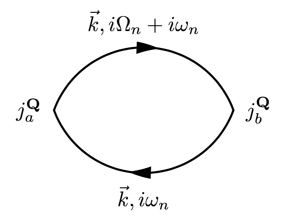
Figure 1: The bare fermion bubble required to be evaluated for $\kappa_{ab}$

For the evaluation of the conductivity, it is useful to express the Green’s function in terms of the spectral representation (for associated subtleties which are irrelevant for us because our order parameters are real, see the appendix of Ref. Durst and Sachdev, 2009),

$$G({\mathbf{k}},i\omega_{n})=\int_{-\infty}^{\infty}d\omega_{1}\;\frac{A({\mathbf{k}},\omega_{1})}{i\omega_{n}-\omega_{1}},\text{ where }A({\mathbf{k}},\omega_{1})=-\frac{1}{\pi}G^{\prime\prime}_{ret}({\mathbf{k}},\omega_{1}).$$ (24)

Plugging this into Eq. (23), we find

$$\Pi_{\kappa}(i\Omega_{n})=\int^{{}^{\prime}}\frac{d^{2}k}{(2\pi)^{2}}\int d\omega_{1}\int d\omega_{2}\,S(i\Omega_{n})\,\text{Tr}\left[A({\mathbf{k}},\omega_{1})\mathbf{V}_{{\mathbf{k}}}A({\mathbf{k}},\omega_{2})\mathbf{V}_{{\mathbf{k}}}\right],$$ (25)

where

$$S(i\Omega_{n})=\frac{1}{\beta}\sum_{i\omega_{n}}\left(i\omega_{n}+\frac{i\Omega_{n}}{2}\right)^{2}\frac{1}{i\omega_{n}-\omega_{1}}\frac{1}{i\omega_{n}+i\Omega_{n}-\omega_{2}}.$$ (26)

The apparent divergence of the Matsubara sum in Eq. (26) is a consequence of the improper treatment of time ordering and time derivatives, which do not commute. A more careful treatment Ambegaokar and Griffin (1965) shows that these issues can safely be ignored and Eq. (26) yields

$$S_{ret}(\Omega)=S(i\Omega\rightarrow\Omega+i0^{+}) = \frac{\left(\omega_{1}+\frac{\Omega}{2}\right)^{2}n_{F}(\omega_{1})-\left(\omega_{2}-\frac{\Omega}{2}\right)^{2}n_{F}(\omega_{2})}{\omega_{1}-\omega_{2}+\Omega+i0^{+}}.$$ (27)

Exploiting this result, we obtain

$$\text{Im}\left[\overset{\leftrightarrow}{\Pi^{R}_{\kappa}}(\Omega)\right]=\int^{{}^{\prime}}\frac{d^{2}k}{4\pi}\int d\omega\left(\omega+\frac{\Omega}{2}\right)^{2}(n_{F}(\omega+\Omega)-n_{F}(\omega))\text{Tr}\left[A({\mathbf{k}},\omega)\mathbf{V}_{{\mathbf{k}}}A({\mathbf{k}},\omega+\Omega)\mathbf{V}_{{\mathbf{k}}}\right]$$

for the imaginary part of the retarded polarization bubble. The real part of the polarization bubble can in principle be calculated using a Kramers-Kronig transformation, but is not required for the computation of the dc thermal conductivity.

In the static limit, where $\Omega\rightarrow 0$, we can replace $(n_{F}(\omega+\Omega)-n_{F}(\omega))\rightarrow\Omega\,n_{F}^{\prime}(\omega)$, canceling the factor of $\Omega$ in the denominator of Eq. (21). Subsequently, we can set $\Omega=0$ everywhere else and obtain in this limit

$$\frac{\overset{\leftrightarrow}{\kappa}(\Omega\rightarrow 0,T)}{T}=\int^{{}^{\prime}}\frac{d^{2}k}{4\pi}\int d\omega\left(\frac{\omega}{T}\right)^{2}\left(-n_{F}^{\prime}(\omega)\right)\text{Tr}\left[A({\mathbf{k}},\omega)\mathbf{V}_{{\mathbf{k}}}A({\mathbf{k}},\omega)\mathbf{V}_{{\mathbf{k}}}\right].$$ (29)

In the scenarios we are interested in, the relevant energy scales $T$ and $\Gamma$ are all much smaller than the Fermi energy $E_{F}$. As the derivative of the Fermi function is strongly peaked at $\omega=0$, for low $T\ll\Gamma\ll E_{F}$, we can set $\omega=0$ in the spectral functions, and evaluate the frequency integral analytically, obtaining

$$\int_{-\infty}^{\infty}d\omega\left(\frac{\omega}{T}\right)^{2}\left(-n_{F}^{\prime}(\omega)\right)=\frac{\pi^{2}k_{B}^{2}}{3}$$ (30)

In this limit, the conductivity takes the form:

$$\frac{\overset{\leftrightarrow}{\kappa}(\Omega\rightarrow 0,T)}{T}=\frac{k_{B}^{2}}{3}\int^{{}^{\prime}}\frac{d^{2}k}{4\pi}\text{Tr}\left[G_{R}^{\prime\prime}({\mathbf{k}},0)\mathbf{V}_{{\mathbf{k}}}G_{R}^{\prime\prime}({\mathbf{k}},0)\mathbf{V}_{{\mathbf{k}}}\right]$$ (31)

where $G_{R}^{\prime\prime}({\mathbf{k}},0)$ is the imaginary part of the retarded Green’s function and the momentum integral is over the (reduced) Brillouin zone. For arbitrary disorder strength, this expression is difficult to evaluate analytically. In certain limits, we can make analytic progress and determine for example whether the Wiedemann-Franz law is satisfied. These analytic calculations will be complemented with numerical results.

III Antiferromagnetic metal

III.1 Thermal conductivity in the spiral and Néel states

In this section, we focus on the dirty limit, where the disorder scattering strength is much stronger than the superconducting order, i. e., the regime where $\Gamma\gg\Delta_{0}$. In this limit, we can neglect superconductivity entirely, and therefore the problem reduces to the computation of the thermal conductivity in an antiferromagnetic metal. We proceed as described in Sec. II.

An antiferromagnetic state with ordering wave vector ${\mathbf{Q}}$ can be described by the Hamiltonian

$$H_{afm} = \sum_{{\mathbf{k}},\sigma=\uparrow,\downarrow}\xi_{{\mathbf{k}}}c^{\dagger}_{{\mathbf{k}}\sigma}c_{{\mathbf{k}}\alpha}-A\sum_{\boldsymbol{k}}\left(c^{\dagger}_{{\mathbf{k}}\uparrow}c_{{\mathbf{k}}+{\mathbf{Q}}\downarrow}+c^{\dagger}_{{\mathbf{k}}+{\mathbf{Q}}\downarrow}c_{{\mathbf{k}}\uparrow}\right)$$

$$= \sum_{{\mathbf{k}}}\Psi^{\dagger}_{{\mathbf{k}}}h_{{\mathbf{k}}}\Psi_{{\mathbf{k}}}\text{ with }h({\mathbf{k}})=\begin{pmatrix}\xi_{{\mathbf{k}}}&-A\\ -A&-\xi_{{\mathbf{k}}}\end{pmatrix}\text{ and }\Psi_{{\mathbf{k}}}=\begin{pmatrix}c_{{\mathbf{k}}\uparrow}\\ c_{{\mathbf{k}}+{\mathbf{Q}}\downarrow}\end{pmatrix}$$

The Green’s function is given by

$$G_{0}({\mathbf{k}},i\omega_{n})=(i\omega_{n}-h_{{\mathbf{k}}})^{-1}=\frac{1}{(i\omega_{n}-E_{+{\mathbf{k}}})(i\omega_{n}-E_{-{\mathbf{k}}})}\begin{pmatrix}i\omega_{n}-\xi_{{\mathbf{k}}}&A\\ A&i\omega_{n}-\xi_{{\mathbf{k}}+{\mathbf{Q}}}\end{pmatrix}$$ (33)

where

$$E_{\pm,{\mathbf{k}}}=\frac{\xi_{{\mathbf{k}}}+\xi_{{\mathbf{k}}+{\mathbf{Q}}}}{2}\pm\sqrt{\left(\frac{\xi_{{\mathbf{k}}}-\xi_{{\mathbf{k}}+{\mathbf{Q}}}}{2}\right)^{2}+A^{2}}$$ (34)

are the two reconstructed bands. An example for the quasi-particle Fermi surface and spectral function of this Hamiltonian is shown in Fig. 2 Eberlein et al. (2016).

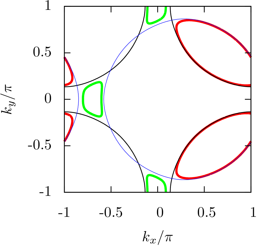
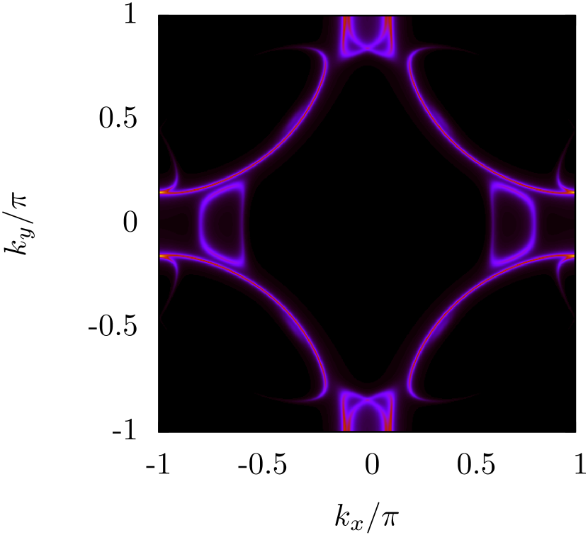
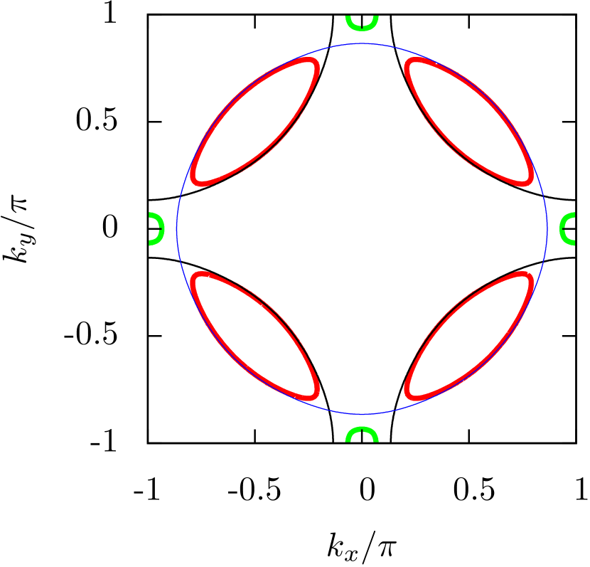
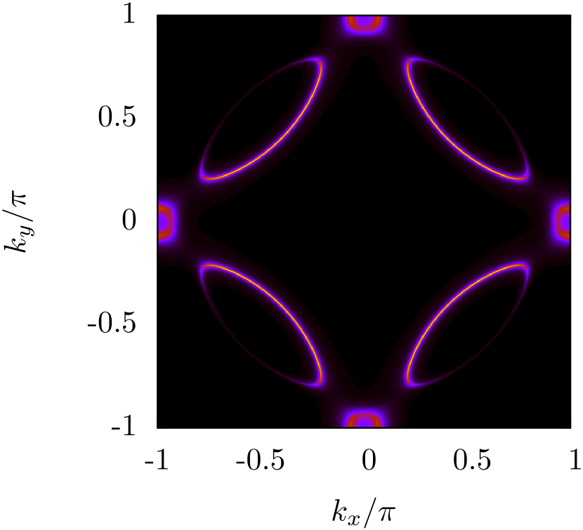
Figure 2: Quasi-particle Fermi surface (left) and spectral function (right) of spiral (top row) and commensurate (bottom row) antiferromagnetic states with $t^{\prime}=-0.35$, $A=0.267$, $p=0.152$ and $\eta\approx p$ ($\eta=0$) for the spiral (commensurate) AF state. In the left figures, hole and electron pockets are marked in red and green, respectively. The thin black and blue lines are the original and $\boldsymbol{Q}$-shifted Fermi surfaces.

For the transport calculation, disorder is added to the Green’s function as described in Eq (19). In the spiral state, the momenta and the spins of the quasiparticles are tied together. This may in general lead to a momentum and spin dependence of the scattering rate even for potential disorder. However, since each state can get scattered to any other state on the Fermi surface by repeated scattering, we assume that the averaged scattering cross-section is roughly the same for any given momenta on the Fermi surface. Therefore, we use a simple retarded self-energy $\Sigma_{R}(\omega\rightarrow 0)=-i\Gamma$ to account for the broadening of the quasiparticle spectrum near the Fermi surface.

The heat conductivity is then evaluated using Eq. (31), using the imaginary part of Eq. (33) after continuation to the real frequency axis, $i\omega_{n}\rightarrow\omega+i\delta$,

$$\text{Im}\left[G^{R}({\mathbf{k}},\omega\rightarrow 0)\right]=\frac{\Gamma}{G_{den}}\left[-\left((E_{+{\mathbf{k}}}^{2}+E_{-{\mathbf{k}}}^{2})/2+\Gamma^{2}\right)\tau_{0}+\Gamma(E_{+{\mathbf{k}}}+E_{-{\mathbf{k}}})\left(A\,\tau_{1}-\frac{(\xi_{{\mathbf{k}}}-\xi_{{\mathbf{k}}+{\mathbf{Q}}})}{2}\,\tau_{3}\right)\right],$$ (35)

where $G_{den}=(E_{+{\mathbf{k}}}E_{-{\mathbf{k}}}-\Gamma^{2})^{2}+\Gamma^{2}\left(E_{+{\mathbf{k}}}+E_{-{\mathbf{k}}}\right)^{2}$, $\tau_{i}$ are the Pauli matrices; and the velocity matrix,

$$\mathbf{V}_{{\mathbf{k}}}=\begin{pmatrix}\mathbf{v}({\mathbf{k}})&0\\ 0&\mathbf{v}({\mathbf{k}}+{\mathbf{Q}})\end{pmatrix}$$ (36)

with appropriate ${\mathbf{Q}}$ for the antiferromagnetic state under consideration. This yields the thermal current operator in Eq. (17) with ${\mathbf{j}}^{Q}_{2}=0$. Note that the momentum integral in Eq. (31) is over the whole Brillouin zone for a spiral antiferromagnetic metal.

This expression needs to be evaluated numerically, but we can simplify it to some extent in the limit where the disorder strength $\Gamma$ is smaller than all the other relevant energy scales, the amplitude of the antiferromagnetic order $A$ and the Fermi energy $E_{F}$ (but it is still larger than $\Delta_{d}$). The final expression, which we do not state here, involves an integral along the Fermi pockets, and is inversely proportional to the scattering rate $\Gamma$.

III.2 Electrical conductivity and the Wiedemann-Franz Law

In this section we evaluate the electrical conductivity for the dirty metal with Néel or spiral order, and show that the Wiedemann Franz law for transport holds. The electric current operator is given by:

$${\mathbf{j}}^{e}({\mathbf{q}}\rightarrow 0,\Omega) = \sum_{{\mathbf{k}},\omega,\sigma}\frac{\partial\xi_{{\mathbf{k}}}}{\partial{\mathbf{k}}}\;c^{\dagger}_{\sigma}({\mathbf{k}},\omega)c_{\sigma}({\mathbf{k}},\omega)=\sum_{{\mathbf{k}},\omega}\Psi^{\dagger}_{k}\mathbf{V}_{{\mathbf{k}}}\Psi_{k+q},$$

$$\text{ where }\mathbf{V}_{{\mathbf{k}}} = \begin{pmatrix}\mathbf{v}({\mathbf{k}})&0\\ 0&\mathbf{v}({\mathbf{k}}+{\mathbf{Q}})\end{pmatrix}$$ (37)

The Kubo formula for the electrical conductivity is given by:

$$\overset{\leftrightarrow}{\sigma}(\Omega,T)=-\underset{\Omega\rightarrow 0}{\text{lim}}\frac{\text{Im }\left[\overset{\leftrightarrow}{\Pi^{R}_{e}}(\Omega)\right]}{\Omega}$$ (38)

where $\Pi^{R}_{e}(\Omega)$ is the retarded current-current correlation function for the electrical current, obtained via analytic continuation from the Matsubara correlation:

$$\Pi^{R}_{e}(\Omega)=\Pi_{e}(i\Omega_{n}\rightarrow\Omega+i0^{+})$$ (39)

Neglecting vertex corrections, we evaluate the bare-bubble contribution to the current-current correlator:

$$\Pi_{e}(i\Omega_{n})=\frac{1}{\beta}\sum_{i\omega_{n},{\mathbf{k}}}\text{Tr}\left[G({\mathbf{k}},i\omega_{n})\mathbf{V}_{{\mathbf{k}}}G({\mathbf{k}},i\omega_{n}+i\Omega_{n})\mathbf{V}_{{\mathbf{k}}}\right]$$ (40)

Using the spectral representation of the Green’s function in Eq. (40), we find:

$$\Pi_{e}(i\Omega_{n})=\int\frac{d^{2}k}{(2\pi)^{2}}\int d\omega_{1}\int d\omega_{2}\,S(i\Omega_{n})\,\text{Tr}\left[A({\mathbf{k}},\omega_{1})\mathbf{V}_{{\mathbf{k}}}A({\mathbf{k}},\omega_{2})\mathbf{V}_{{\mathbf{k}}}\right]$$ (41)

where

$$S(i\Omega_{n})=\frac{1}{\beta}\sum_{i\omega_{n}}\frac{1}{i\omega_{n}-\omega_{1}}\frac{1}{i\omega_{n}+i\Omega_{n}-\omega_{2}}$$ (42)

The Matsubara sum is convergent, and evaluates to:

$$S_{ret}(\Omega)=S(i\Omega\rightarrow\Omega+i0^{+}) = \frac{n_{F}(\omega_{1})-n_{F}(\omega_{2})}{\omega_{1}-\omega_{2}+\Omega+i0^{+}}$$

$$\implies\text{Im}\left[S_{ret}(\Omega))\right] = \pi(n_{F}(\omega_{1}+\Omega)-n_{F}(\omega_{1}))\,\delta(\omega_{1}-\omega_{2}+\Omega)$$ (43)

The imaginary part of retarded polarization bubble is therefore given by:

$$\text{Im}\left[\overset{\leftrightarrow}{\Pi^{R}_{e}}(\Omega)\right]=\int\frac{d^{2}k}{4\pi}\int d\omega(n_{F}(\omega+\Omega)-n_{F}(\omega))\text{Tr}\left[A({\mathbf{k}},\omega)\mathbf{V}_{{\mathbf{k}}}A({\mathbf{k}},\omega+\Omega)\mathbf{V}_{{\mathbf{k}}}\right]$$ (44)

Assuming that $T\rightarrow 0$, we can approximate the derivative of the Fermi function by a delta function as $\Omega\rightarrow 0$ in the dc limit:

$$(n_{F}(\omega+\Omega)-n_{F}(\omega))/\Omega\approx\delta(\omega)$$ (45)

Using this to evaluate the $\omega$ integral, we end up with the following expression for the electrical conductivity:

$$\overset{\leftrightarrow}{\sigma}(\Omega\rightarrow 0,T\rightarrow 0)=\frac{e^{2}}{\pi^{2}}\int\frac{d^{2}k}{4\pi}\text{Tr}\left[G_{R}^{\prime\prime}({\mathbf{k}},0)\mathbf{V}_{{\mathbf{k}}}G_{R}^{\prime\prime}({\mathbf{k}},0)\mathbf{V}_{{\mathbf{k}}}\right]$$ (46)

Comparing Eq. (46) with Eq. (31), we find that the Wiedemann-Franz law is obeyed, as one would expect for a quasiparticle Fermi surface with constant scattering lifetime:

$$\frac{\kappa}{\sigma T}=\frac{\pi^{2}k_{B}^{2}}{3e^{2}}$$ (47)

III.3 Numerical results for antiferromagnetic metals

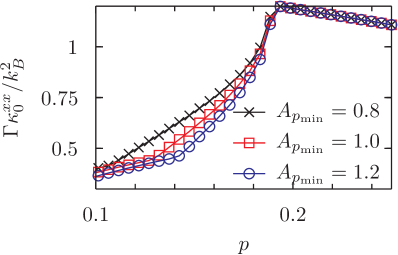
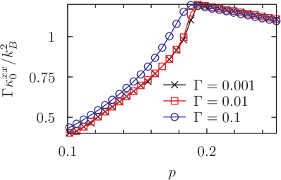
Figure 3: Influence of the size of the spiral antiferromagnetic gap $A$ (left) and the scattering rate $\Gamma$ (right) on the heat conductivity for $t^{\prime}=-0.35$. and $\Gamma=0.01$. Antiferromagnetism disappears at $p^{\ast}=0.19$. In the left plot we use $\Gamma=0.01$ and in the right plot the gap at $p=0.05$ is set to $A_{p_{\text{min}}}=0.8$.

In the following we discuss numerical results for

$$\kappa_{0}=\lim_{T\rightarrow 0}\frac{\kappa_{xx}(\Omega\rightarrow 0,T)}{T}$$ (48)

in the presence of (in-) commensurate antiferromagnetic order. The latter is described by an antiferromagnetic gap with the phenomenological doping dependence

$$A(p)=A_{0}(p^{*}-p)\Theta(p^{*}-p),$$ (49)

where $A_{0}$ is fixed by the antiferromagnetic gap $A_{p_{\text{min}}}$ at the smallest doping considered, $p_{\text{min}}=0.05$ and $p^{*}=0.19$ is the critical doping beyond which antiferromagnetic order disappears. In this section, we set $t^{\prime}=-0.35$. In Fig. 3 we show the influence of the size of the antiferromagnetic gap on the heat conductivity. Similarly to the Hall coefficient near an antiferromagnetic phase transition Storey (2016); Eberlein et al. (2016), the magnitude of the spiral order parameter mostly influences the width of the crossover region, in which electron and hole pockets coexist. With increasing strength of antiferromagnetic order, the transition region shrinks. In Fig. 3, we show the influence of the size of $\Gamma$ on the doping dependence of the heat conductivity. We plot $\Gamma\kappa_{0}$ for better comparison. For the smallest value, $\Gamma=0.001$, the results are indistinguishable from those obtained in a relaxation time approximation in which $\Gamma\rightarrow 0$ is assumed, as employed in Ref. Eberlein et al., 2016. The doping dependence of $\Gamma\kappa_{0}$ is only altered at large values of $\Gamma$, as shown in Fig. 3.

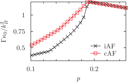
Figure 4: Comparison of the doping dependence of the heat conductivity for commensurate (cAF) and incommensurate (iAF) antiferromagnetism for $p<p^{\ast}$ for $t^{\prime}=-0.35$ and $A_{p_{\text{min}}}=1.0$. Antiferromagnetism disappears at $p^{\ast}=0.19$. We plot $\Gamma\kappa_{0}$ for better comparison.

In Fig. 4, we compare the doping dependence of the heat conductivity for commensurate or incommensurate antiferromagnetism for $p<p^{\ast}$. In the incommensurate case, the heat conductivity drops significantly faster for $p<p^{\ast}$ than in the commensurate case. This difference can be understood analytically and is discussed in the next section.

Collignon et al. found that the drop in the electrical conductivity can be entirely understood as a drop in the charge carrier density when assuming that the charge carrier mobility is constant across the phase transition Collignon et al. (2017). Evidence for a constant mobility is found in the behavior of the Hall angle and the magnetoresistance. The charge carrier density can then be extracted from the heat or electrical conductivity via

$$p_{\sigma}=(1+p)\frac{\sigma(0)}{\sigma_{0}}$$ (50)

where $\sigma_{0}$ ($\sigma(0)$) is the conductivity in the absence (presence) of antiferromagnetic order. In experiments, $\sigma_{0}$ is obtained by extrapolating the conductivity from high to low temperatures.

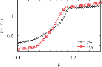
Figure 5: Effective charge carrier density as extracted from the heat conductivity in comparison to the Hall number for a phase transition to incommensurate antiferromagnetic order. Parameters are $t^{\prime}=-0.35$ and $A_{p_{\text{min}}}=1.0$. $\Gamma=0.001$ in the computation of the conductivity. The Hall number was determined in the relaxation time approximation as described in Ref. Eberlein et al. (2016).

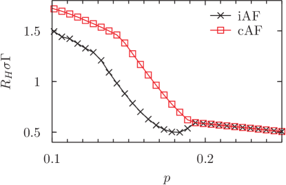
Figure 6: Doping dependence of the Hall angle $R_{H}\sigma$, rescaled by $\Gamma$, across a phase transition from a paramagnetic to an (in-) commensurate antiferromagnetic metal with $A_{p_{\text{min}}}=1.0$ in both cases.

For our calculation we assume that the disorder scattering rate is independent of doping and do not make assumptions on the mobility. This leads to a behavior of $p_{\sigma}$ that is distinct from that of the Hall coefficient, as shown in Fig. 5, and is connected to the fact that the drop in the conductivity is smaller than the drop in the Hall number. In Fig. 6, we plot the Hall angle across the phase transition to (in-) commensurate antiferromagnetism. For commensurate antiferromagnetism, the Hall angle increases for $p<p^{\ast}$. In the incommensurate case, there is a slight drop of $R_{H}\sigma$ below the critical point before it starts to increase. It is interesting to compare this behavior to the experimental results by Collignon et al. Collignon et al. (2017) on Nd-LSCO. In Fig. 10 of their paper the Hall angle is shown to drop by a factor of three (approximately) within a small doping range. This is attributed to Fermi surface reconstruction below $p^{\ast}$ and appearance of electron-like pockets. In our model the relative drop is smaller, and in Sec. V we demonstrate how a doping dependent scattering rate can alleviate this discrepancy.

III.4 Analytic understanding of the numerical results

In this section, we estimate the drop of the conductivity across the phase transition. Our estimates are valid for the weakly disordered antiferromagnetic metal, or coexisting antiferromagnetism and superconductivity in the dirty limit ($\Delta\ll\Gamma$) and capture the change quite well. Instead of the thermal conductivity, we focus on the diagonal electrical conductivity as in this regime the Wiedemann-Franz law is obeyed.

In our mean-field model, the Fermi velocity $v_{F}$ is unrenormalized across the phase transition on most parts of the Fermi surface, except close to the points that get gapped out (near the edges of the pockets). Therefore, the electrical conductivity can be approximated as:

$$\sigma_{xx}\sim\int_{{\mathbf{k}}}\left(\frac{\partial E_{{\mathbf{k}}}}{\partial k_{x}}\right)^{2}n_{F}^{\prime}(E_{{\mathbf{k}}})\approx\int_{{\mathbf{k}}}({\mathbf{v}_{F}}_{x})^{2}\delta\left({\mathbf{v}_{F}}({\mathbf{k}})\cdot({\mathbf{k}}-{\mathbf{k}}_{F})\right)$$ (51)

$$\approx\left<\frac{v_{F,x}^{2}}{v_{F}}\right>\times\text{Total perimeter of Fermi surface/pockets}.$$ (52)

We have also assumed that scattering is mainly due to disorder, so that the quasi-particle scattering rate is unchanged across the transition.

In absence of antiferromagnetic order, we have a large hole-like Fermi surface of size $1+p$, which accommodates both spin species. We assume that this pocket is circular with radius $k_{F}$, so that the density of holes is given by (setting lattice spacing $a=1$):

$$2\times\frac{\pi k_{F}^{2}}{(2\pi)^{2}}=1+p\implies k_{F}=\sqrt{2\pi(1+p)}.$$ (53)

This implies that the diagonal conductivity is given by (modulo constant factors):

$$\sigma_{Large\,FS}\sim\left<\frac{v_{F,x}^{2}}{v_{F}}\right>\times 2\times 2\pi k_{F}=4\pi\left<\frac{v_{F,x}^{2}}{v_{F}}\right>\sqrt{2\pi(1+p)}$$ (54)

Antiferromagnetic order leads to reconstruction of the large Fermi surface into electron and hole pockets. In the following we assume that the antiferromagnetic order parameter is large enough to gap out the electron pockets. In the presence of Néel order, we have four hole pockets in the large Brillouin zone (taking spin already into account). For the spiral order there are only two somewhat larger hole pockets, see Figs. 2. These pockets are approximately elliptic, with an eccentricity of $e\approx 0.5$ in both cases. The area of the ellipse is given by $\pi K_{1}K_{2}=\pi K_{1}^{2}/2$, where $K_{1}$($K_{2}$) is the semi-major(minor) axis of the ellipse. The perimeter of a single elliptical pocket is given by

$$S_{ellipse}=4K_{1}\int_{0}^{\pi/2}d\theta\sqrt{1-e^{2}\text{ sin}^{2}\theta}~{}\approx 6K_{1},\text{ for }e=0.5.$$ (55)

For the Néel ordered case, we find

$$4\times\frac{\pi K_{1}^{2}}{2(2\pi)^{2}}=p\implies K_{1}=\sqrt{2\pi p},$$ (56)

so that the diagonal conductivity is given by

$$\sigma_{\text{N\'{e}el}}\sim\left<\frac{v_{F,x}^{2}}{v_{F}}\right>\times 4\times 6K_{1}=24\left<\frac{v_{F,x}^{2}}{v_{F}}\right>\sqrt{2\pi p}.$$ (57)

For spiral order, we have

$$2\times\frac{\pi K_{1}^{2}}{2(2\pi)^{2}}=p\implies K_{1}=2\sqrt{\pi p}$$ (58)

and can estimate the conductivity as

$$\sigma_{iAF}\sim\left<\frac{v_{F,x}^{2}}{v_{F}}\right>\times 2\times 6K_{1}=24\left<\frac{v_{F,x}^{2}}{v_{F}}\right>\sqrt{\pi p}.$$ (59)

We estimate the drop of the conductivity across the phase transition by comparing the results for the large Fermi surface at a doping $p_{1}=0.2$ with the result for the small Fermi pockets at $p_{2}=0.1$. For Néel order we find

$$\frac{\sigma_{\text{N\'{e}el}}}{\sigma_{Large\,FS}}=\frac{6}{\pi}\sqrt{\frac{p_{2}}{1+p_{1}}}=\frac{\sqrt{3}}{\pi}\approx 0.55,$$ (60)

while for spiral order we obtain

$$\frac{\sigma_{iAF}}{\sigma_{Large\,FS}}=\frac{6}{\pi}\sqrt{\frac{p_{2}}{2(1+p_{1})}}\approx 0.39$$ (61)

Both of these seem to agree quite well with the numerical data, as does the approximation that $\sigma_{\text{N\'{e}el}}/\sigma_{\text{iAF}}=\sqrt{2}$ at the same doping $p_{2}$ after the disappearance of the electron pockets.

IV Co-existing antiferromagnetism and superconductivity

In this section, we discuss the thermal conductivity for co-existing antiferromagnetic and superconducting order. This is motivated by the fact that most transport experiments at low temperatures are done in the superconducting phase. The reason is that the experimentally accessible magnetic fields do not suffice to suppress superconductivity completely in most materials. Therefore it is interesting to ask which experimental signatures of incommensurate antiferromagnetic or topological order could show up in transport measurements in the superconducting phase. We consider both commensurate (Néel) and incommensurate (spiral) antiferromagnetic order. Since the formalism has a significant amount of overlap for these two scenarios, we combine them into a single section, with separate subsections where the results differ significantly.

IV.1 Spectrum

Commensurate and incommensurate antiferromagnetism coexisting with superconductivity can be described by the mean-field Hamiltonian in Eq. (1) Yamase et al. (2016). For convenience of calculation, we re-write it in terms of a $4\times 4$ Nambu notation, with

$$H_{\text{AF+dSC}}=\sum_{{\mathbf{k}}}^{\prime}\Psi^{\dagger}_{{\mathbf{k}}}h({\mathbf{k}})\Psi_{{\mathbf{k}}},\text{ with }h({\mathbf{k}})=\begin{pmatrix}\xi_{{\mathbf{k}}}&\Delta_{{\mathbf{k}}}&-A&0\\ \Delta_{{\mathbf{k}}}&-\xi_{{\mathbf{k}}}&0&A\\ -A&0&\xi_{{\mathbf{k}}+{\mathbf{Q}}}&-\Delta_{{\mathbf{k}}+{\mathbf{Q}}}\\ 0&A&-\Delta_{{\mathbf{k}}+{\mathbf{Q}}}&-\xi_{{\mathbf{k}}+{\mathbf{Q}}}\end{pmatrix}\text{ and }\Psi_{{\mathbf{k}}}=\begin{pmatrix}c_{{\mathbf{k}}\uparrow}\\ c^{\dagger}_{-{\mathbf{k}}\downarrow}\\ c_{{\mathbf{k}}+{\mathbf{Q}}\downarrow}\\ c^{\dagger}_{-{\mathbf{k}}-{\mathbf{Q}}\uparrow}.\end{pmatrix}$$

Here we have assumed that the electron dispersion $\xi_{{\mathbf{k}}}$ is symmetric under spatial inversion, ${\mathbf{k}}\rightarrow-{\mathbf{k}}$. The sum over momenta $\boldsymbol{k}$ is restricted to $-\pi<k_{x}\leq\pi$ and $-\pi/2<k_{y}\leq\pi/2$ in order to avoid double counting. We have checked explicitly that the mean-field Hamiltonian can be rewritten in the spinor notation by employing all allowed operations (like shifting the $x$-component of momenta, inverting momenta, but not shifting the $y$-component of momenta after introducing the reduced BZ). For general ${\mathbf{Q}}$, the eigenvalues of $h({\mathbf{k}})$ are given by:

$$E_{\pm,{\mathbf{k}}}^{2} = \frac{1}{2}\left(2A^{2}+\Lambda_{{\mathbf{k}}}\pm\sqrt{\alpha_{{\mathbf{k}}}^{2}+4A^{2}\beta_{{\mathbf{k}}}}\right),\text{ where }$$

$$\Lambda_{{\mathbf{k}}} = \Delta_{{\mathbf{k}}}^{2}+\Delta_{{\mathbf{k}}+{\mathbf{Q}}}^{2}+\xi_{{\mathbf{k}}}^{2}+\xi_{{\mathbf{k}}+{\mathbf{Q}}}^{2},\,\alpha_{{\mathbf{k}}}=\Delta_{{\mathbf{k}}}^{2}-\Delta_{{\mathbf{k}}+{\mathbf{Q}}}^{2}+\xi_{{\mathbf{k}}}^{2}-\xi_{{\mathbf{k}}+{\mathbf{Q}}}^{2},\text{ and }$$

$$\beta_{{\mathbf{k}}} = \left(\Delta_{{\mathbf{k}}}+\Delta_{{\mathbf{k}}+{\mathbf{Q}}}\right)^{2}+\left(\xi_{{\mathbf{k}}}+\xi_{{\mathbf{k}}+{\mathbf{Q}}}\right)^{2}$$ (63)

Setting $\Delta_{{\mathbf{k}}}=0$, we recover the spectrum of the antiferromagnetic metal Schulz (1990). For $A=0$, we recover the spectrum of a superconductor $E^{0}_{{\mathbf{k}}}$ and $E^{0}_{{\mathbf{k}}+{\mathbf{Q}}}$, where $E^{0}_{{\mathbf{k}}}=\sqrt{\xi_{{\mathbf{k}}}^{2}+\Delta_{{\mathbf{k}}}^{2}}$. These two branches together count the states of the uniform superconductor in the full BZ, as there is no translation symmetry breaking for $A=0$.

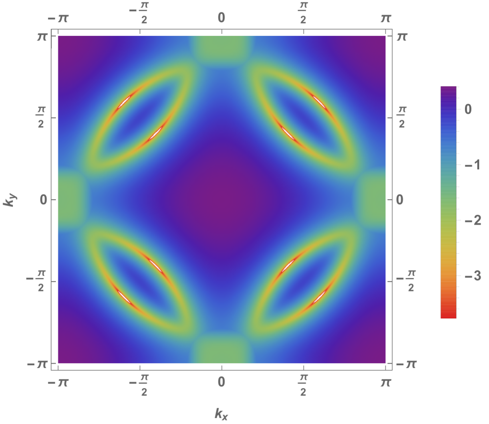
(a)

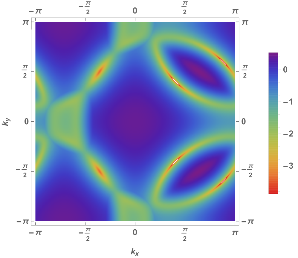
(b)

Figure 7: Plots of logarithm of the dispersions of the lower band (a.u.) at $p=0.152$, for parameter values $t^{\prime}=-0.35,\mu=-1.099,\Delta_{d}=0.1,A=0.267$, and $\eta=0$ for Néel and $0.1436$ for spiral order. (a) Néel order + superconductivity: Eight nodes in the extended BZ. (b) Spiral order + superconductivity: Four nodes in the extended BZ.

We choose the superconducting gap to have $d$-wave symmetry, as appropriate for cuprate superconductors and theoretical models of antiferromagnetism coexisting with superconductivity Halboth and Metzner (2000); Maier et al. (2000); Lichtenstein and Katsnelson (2000); Sushkov and Kotov (2004); Maier et al. (2005); Capone and Kotliar (2006); Aichhorn et al. (2006); Khatami et al. (2008); Kancharla et al. (2008); Friederich et al. (2011); Gull et al. (2013); Eberlein and Metzner (2014); Rømer et al. (2016); Yamase et al. (2016); Zheng and Chan (2016). The dispersion in Eq. (63) then possesses gapless nodal excitations. In Fig. 7, we plot the spectrum of the Néel and spiral states coexisting with superconductivity. We note that the Néel ordered superconductor has eight nodal points in the extended BZ, whereas the superconductor with spiral order has only four nodes.

IV.2 Thermal conductivity

The bare Matsubara Green’s function is in the Nambu basis described above is given by:

$$G^{0}({\mathbf{k}},i\omega_{n})=\left(i\omega_{n}-h_{{\mathbf{k}}}\right)^{-1}$$ (64)

Now we add impurity contribution to the self-energy, which is a $4\times 4$ matrix $\hat{\Sigma}(i\omega_{n})$ in Nambu space in full generality. We only consider the scalar term for simplicity, which allows us to write down the dressed Green’s function in terms of the bare one as follows:

$$\begin{split}G^{-1}({\mathbf{k}},i\omega_{n})&=[G^{0}({\mathbf{k}},i\omega_{n})]^{-1}-\hat{\Sigma}(i\omega_{n})\approx[G^{0}({\mathbf{k}},i\omega_{n})]^{-1}-\Sigma(i\omega_{n})\mathbb{I}_{4\times 4}\\ &=[G^{0}({\mathbf{k}},i\omega_{n}-\Sigma(i\omega_{n}))]^{-1}\end{split}$$ (65)

Following analytic continuation to real frequencies, $\Sigma_{R}(0)=-i\Gamma$, the imaginary part of the retarded Green’s function in the $\omega\rightarrow 0$ limit can be expressed as follows in terms of Pauli matrices $\tau_{i}$ and the $2\times 2$ identity matrix $\tau_{0}$ (relabeling ${\mathbf{k}}$ as 1 and ${\mathbf{k}}+{\mathbf{Q}}$ as 2):

$$\text{Im}[G_{R}({\mathbf{k}},\omega\rightarrow 0)] = \frac{1}{G_{den}}\begin{pmatrix}G_{a}^{\prime\prime}&G_{b}^{\prime\prime}\\ G_{c}^{\prime\prime}&G_{d}^{\prime\prime}\end{pmatrix},\text{ where}$$

$$G_{a}^{\prime\prime} = -\Gamma(\Gamma^{2}+A^{2}+\xi_{2}^{2}+\Delta_{2}^{2})\,\tau_{0}$$

$$G_{b}^{\prime\prime} = -A\Gamma\left[(\xi_{1}+\xi_{2})-(\Delta_{1}+\Delta_{2})(i\tau_{2})\right]$$

$$G_{c}^{\prime\prime} = -A\Gamma\left[(\xi_{1}+\xi_{2})+(\Delta_{1}+\Delta_{2})(i\tau_{2})\right]$$

$$G_{d}^{\prime\prime} = -\Gamma(\Gamma^{2}+A^{2}+\xi_{1}^{2}+\Delta_{1}^{2})\,\tau_{0}$$

$$G_{den} = (\Gamma^{2}+A^{2}+\xi_{1}^{2}+\Delta_{1}^{2})(\Gamma^{2}+A^{2}+\xi_{2}^{2}+\Delta_{2}^{2})-A^{2}\left[(\xi_{1}+\xi_{2})^{2}+(\Delta_{1}+\Delta_{2})^{2}\right]$$

Noting that ${\mathbf{v}_{\Delta}}(-{\mathbf{k}})=-{\mathbf{v}_{\Delta}}({\mathbf{k}})$ and working through some algebra, we find that we can write the thermal current operator in terms of the Nambu spinor $\Psi_{{\mathbf{k}}}$ as:

$${\mathbf{j}}^{Q}({\mathbf{q}}\rightarrow 0,\Omega)=\sum_{{\mathbf{k}},\omega}^{\prime}\left(\omega+\frac{\Omega}{2}\right)\Psi^{\dagger}_{k}\mathbf{V}_{{\mathbf{k}}}\psi_{k+q},\text{ where }$$

$$\mathbf{V}_{{\mathbf{k}}}=\begin{pmatrix}{\mathbf{v}_{F}}({\mathbf{k}})\tau_{3}+{\mathbf{v}_{\Delta}}({\mathbf{k}})\tau_{1}&0\\ 0&{\mathbf{v}_{F}}({\mathbf{k}}+{\mathbf{Q}})\tau_{3}-{\mathbf{v}_{\Delta}}({\mathbf{k}}+{\mathbf{Q}})\tau_{1}\end{pmatrix}$$ (67)

Following the procedure outlined in Sec. II.4, we can evaluate the thermal conductivity by extending the summation to the full BZ with an added factor of half:

$$\frac{\overset{\leftrightarrow}{\kappa}(\Omega\rightarrow 0,T)}{T}=\frac{k_{B}^{2}}{3}\int\frac{d^{2}k}{8\pi}\text{Tr}\left[G_{R}^{\prime\prime}({\mathbf{k}},0)\mathbf{V}_{{\mathbf{k}}}G_{R}^{\prime\prime}({\mathbf{k}},0)\mathbf{V}_{{\mathbf{k}}}\right].$$ (68)

For arbitrary disorder strength, we evaluate this expression numerically. In the clean limit, it can be treated analytically so that connections with the universal Durst-Lee result in the absence of magnetism Durst and Lee (2000) can be drawn. This is discussed in the next section.

IV.3 Analytic expressions in the clean limit

IV.3.1 Néel order

For Néel-type antiferromagnetic order coexisting with superconductivity in the clean limit, $\Gamma_{0}\rightarrow 0$, the thermal conductivity can be evaluated analytically. In this case, the major contribution to the thermal current is carried by nodal quasiparticles, again allowing us to linearize the dispersion at each nodal point. We obtain

$$\frac{\kappa_{ii}(\Omega\rightarrow 0,T)}{T}=\frac{k_{B}^{2}}{3v_{F}v_{\Delta}}\bigg{[}\sqrt{1-\alpha^{2}}\,v_{F}^{2}+\frac{1}{\sqrt{1-\alpha^{2}}}v_{\Delta}^{2}\bigg{]}\Theta(1-\alpha),\text{ where }\alpha=\frac{A}{A_{c}}.$$ (69)

For $A\rightarrow 0$, i. e. vanishing antiferromagnetic order, we recover the result by Durst and Lee Durst and Lee (2000) as expected.

Tuning the order parameter $A$ at fixed chemical potential beyond a critical value $A_{c}$, the nodes can collide and become gapped as discussed in Appendix A. This entails an exponential suppression of the heat conductivity due to the resulting gap in the spectrum in the absence of large disorder broadening. This scenario could be relevant in the strongly underdoped regime, as gapping out the nodes leads to a phase transition from a superconductor to a half-filled insulator.

The above result also indicates that close to the doping $p^{\ast}$ where antiferromagnetic order appears, the number of nodes and the nodal velocities remain unaffected across the phase transition. Thus, a smooth behavior of the heat conductivity is expected near $p^{\ast}$, consistent with our numerical results in Fig. 8.

A few further comments are in order. The apparent divergence of $\kappa/T$ for $A\rightarrow A_{c}$ is an artifact of the clean approximation, which will get smoothened out by disorder. Moreover, there is no nematic order (corresponding to the breaking of the $C_{4}$ symmetry of the square lattice to $C_{2}$) and $\kappa_{xx}=\kappa_{yy}$. This is markedly different from the cases of superconductivity coexisting with spiral antiferromagnetism or charge density waves with axial wave-vector Durst and Sachdev (2009). Finally, our result is valid for any anisotropy ratio $v_{F}/v_{\Delta}$, unlike the isotropic limit discussed in Ref. Durst and Sachdev, 2009. The dependence of $\kappa$ on the order parameter magnitude is also different in these two cases, and may be used as a probe to distinguish between these two different orders in a clean $d$-wave superconductor.

Note that although the results in Ref. Durst and Sachdev, 2009 correspond to a s-wave charge density wave, the wave-vector $(\pi,0)$ is obtained considering the second harmonic of the experimentally observed wave-vector of $(\pi/2,0)$. For a $d$-wave bond density wave which has been observed in STM experiments Hamidian et al. (2016), we need to consider the second harmonic which has a squared form factor, i.e, $\psi_{{\mathbf{k}}}\sim(\text{cos}k_{x}-\text{cos}k_{y})^{2}$. Therefore, the equation $\partial_{{\mathbf{k}}}\psi_{{\mathbf{k}}}=0$ still holds at the nodes which lie along $k_{x}=\pm k_{y}$, and their results are valid for the d-form factor density wave state as well.

IV.3.2 Spiral order

For the case of spiral order, the metallic state with no superconductivity has only two hole pockets, which are in the region $k_{x}>0$ for ${\mathbf{Q}}=(\pi-2\pi\eta,\pi)$. This can be understood from the fact that for small $A$, the particle-hole polarization bubble at momentum ${\mathbf{Q}}$ is maximum when ${\mathbf{Q}}$ approximately nests two segments of the Fermi surface, and accordingly the saddle-point free energy for the fluctuations of the order-parameter field after integrating out the fermions is minimum. As we fix the phenomenological doping dependence of the order parameter amplitude $A$ and minimize the free energy by optimizing the incommensurability $\eta$ Eberlein et al. (2016), the preferred $\eta$ gaps out a large part of the Fermi pockets to reduce the mean-field free energy.

Adding superconductivity on top of the spiral state therefore implies that there are only four nodes in the extended BZ, coming from the two hole-pockets. The other four nodes will collide and disappear once spiral order sets in. Thus, in the clean limit we expect the thermal conductivity to drop to half of its original value soon after crossing $p^{\ast}$ from the overdoped side. Evaluating the heat conductivity by focusing on the vicinity of the four nodal points for $p\lesssim p^{*}$, the thermal conductivity for the clean $d$-wave superconductor with spiral order is given by half of the Durst-Lee value,

$$\frac{\kappa_{ii}(\Omega\rightarrow 0,T)}{T}=\frac{k_{B}^{2}(v_{F}^{2}+v_{\Delta}^{2})}{6v_{F}v_{\Delta}}$$ (70)

Indeed, numerical results in Fig. 8 show a sharp drop of the thermal conductivity by a factor of two across the critical point.

IV.4 Violation of the Wiedemann-Franz law

In the clean limit, we can evaluate the bare-bubble electrical conductivity due to gapless nodal quasiparticles as described in section III.2. For Néel order, the non-superfluid contribution to the electrical current is given by:

$${\mathbf{j}}^{e}({\mathbf{q}}\rightarrow 0,\Omega)=\sum_{{\mathbf{k}},\omega}^{\prime}\Psi^{\dagger}_{k}\mathbf{V}_{{\mathbf{k}}}\psi_{k+q},\text{ where }$$

$$\mathbf{V}_{{\mathbf{k}}}=\begin{pmatrix}{\mathbf{v}_{F}}({\mathbf{k}})\tau_{0}&0\\ 0&{\mathbf{v}_{F}}({\mathbf{k}}+{\mathbf{Q}})\tau_{0}\end{pmatrix}\approx\begin{pmatrix}{\mathbf{v}_{F}}({\mathbf{k}})\tau_{0}&0\\ 0&-{\mathbf{v}_{F}}({\mathbf{k}})\tau_{0}\end{pmatrix}$$ (71)

From this, the quasiparticle contribution to the electrical conductivity (denoted by $\tilde{\sigma}$) can be evaluated using an analogous computation to the thermal conductivity:

$$\tilde{\sigma}_{ii}(\Omega\rightarrow 0,T\rightarrow 0) = \frac{e^{2}}{\pi^{2}}\int\frac{d^{2}k}{8\pi}\text{Tr}\left[G_{R}^{\prime\prime}({\mathbf{k}},0)\mathbf{V}_{{\mathbf{k}}}G_{R}^{\prime\prime}({\mathbf{k}},0)\mathbf{V}_{{\mathbf{k}}}\right]$$ (72)

$$= \frac{e^{2}}{\pi^{2}}\frac{v_{F}}{v_{\Delta}}\sqrt{1-\alpha^{2}}\,\Theta(1-\alpha),\text{ where }\alpha=\frac{A}{A_{c}}$$

Therefore, in the clean limit we have:

$$\frac{\kappa}{\tilde{\sigma}T}=\frac{\pi^{2}k_{B}^{2}}{3e^{2}}\left(1+\frac{1}{1-\alpha^{2}}\frac{v_{\Delta}^{2}}{v_{F}^{2}}\right)$$ (73)

Since the Fermi surface is modified as a function of doping, $\alpha$, the Fermi velocity and the gap velocity all change and therefore $\kappa/\tilde{\sigma}T$ is not a constant as a function of doping in the antiferromagnetic ($A\neq 0$) regime. However, typically the Fermi velocity is much larger than the gap velocity, and therefore this correction is expected to be small. As $\alpha\rightarrow 1$, the correction appears large if we hold $v_{\Delta}$ fixed. But this is a rather unphysical limit as increasing antiferromagnetism to its critical value will reduce the superconductivity $\Delta_{d}$, and $v_{\Delta}$ will also drop. Note that for isotropic disorder scattering, the single-particle lifetime is equal to the scattering time for free fermions. Even for our lattice model, we expect only minor modifications from the bare-bubble result due to vertex corrections. In particular, in the dirty limit $v_{\Delta}/v_{F}\rightarrow 0$ and the Wiedemann-Franz law is exactly satisfied by the quasiparticle contribution to the electric current, as long as the disorder is relatively weak compared to the Fermi energy, as described in section III.2.

IV.5 Numerical results

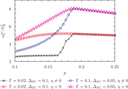
Figure 8: Doping evolution of the heat conductivity in the clean and dirty limits, comparing commensurate and incommensurate antiferromagnetic order. Parameters are $t^{\prime}=-0.35$ and $A_{p_{\text{min}}}=1.0$.

In Fig. 8, we compare the doping dependence of the heat conductivity in the clean and dirty limit for antiferromagnetism coexisting with superconductivity. In the case of commensurate antiferromagnetism, the change near $p^{\ast}$ is less pronounced than in the case of incommensurate antiferromagnetism for both the clean and dirty limits. In the clean limit, the location of $p^{\ast}$ is not discernible from the plot of $\kappa_{0}^{xx}$ in the commensurate case. This is consistent with the analytical result in Eq. (69). In contrast, at the doping where the spiral antiferromagnetic order appears, the heat conductivity drops to roughly half of its value. In the case of incommensurate antiferromagnetism coexisting with superconductivity in the dirty limit, the doping dependence of the heat conductivity is much smoother, as already discussed above. In Fig. 9, we show the evolution of the heat conductivity for various scattering rates from the clean to the dirty limit, demonstrating how the jump gets washed out with increasing scattering rate.

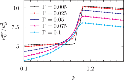
Figure 9: Evolution of heat conductivity from the clean to the dirty limit for coexisting superconductivity and incommensurate antiferromagnetism, for $A_{p_{\text{min}}}=1.0$ and $\Delta=0.05$.

V Influence of doping-dependent scattering in the dirty limit

In Sec. III.4 we discussed that the drop in the thermal conductivity across the antiferromagnetic phase transition can be understood in terms of a reconstruction of the Fermi surface in case of a disordered antiferromagnetic metal or a dirty superconductor ($\Delta_{d}\ll\Gamma$). In this scenario, the relative drop across the phase transition is smaller than the drop of the Hall number, whereas experiments suggest that the drops are of very similar magnitude. The experiments have been interpreted in terms of a Drude-like model, which allows to connect the drop in the conductivity with a drop in the charge-carrier density Collignon et al. (2017) by assuming that the charge carrier mobility is unchanged across the phase transition. However, this requires the validity of an effective mass picture, or nearly circular pockets, which only holds for a very large antiferromagnetic order parameter. Below the optimal doping QCP, the pockets are quite distorted and an effective mass picture is therefore not appropriate. Very recent experiments on electron-doped cuprate LCCO Sarkar et al. (2017) have also observed similar resitivity upturns which cannot be explained only by a drop in carrier density. In this section, we provide an alternative scenario that would explain the larger drop in conductivity.

The key observation is that the scattering rate $\Gamma$ cancels in the Hall number Voruganti et al. (1992); Eberlein et al. (2016), while the thermal conductivity in the dirty superconductor is approximately proportional to $\Gamma^{-1}$. Therefore, one might anticipate that additional sources of scattering that appear once antiferromagnetism sets in can entail a larger drop of the thermal conductivity. We show that a phenomenological doping-dependent scattering rate can indeed lead to similar behavior and drop sizes in the Hall number and the conductivities. We then argue for a possible source of enhanced scattering in the underdoped regime.

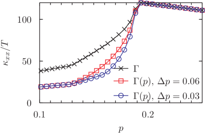
Figure 10: Doping dependence of the heat conductivity for $t^{\prime}=-0.35$, $A_{p_{\text{min}}}=1.0$ and $\Gamma_{0}=0.01$. The curve labeled $\Gamma$ shows the same data as in Fig. 4 for comparison. The other two curves were obtained for a doping dependent scattering rate that doubles over a doping range of $\Delta p$ below $p^{\ast}$.

For simplicity, we assume that the doping dependence of $\Gamma(p)$ is given by

$$\Gamma(p)=\begin{cases}2\Gamma_{0}&\text{for }p<p^{\ast}-\Delta p\\ 2\Gamma_{0}-\Gamma_{0}(p-p^{\ast}+\Delta p)/\Delta p&\text{for }p^{\ast}-\Delta p\leq p\leq p^{\ast}\\ \Gamma_{0}&\text{for }p>p^{\ast},\end{cases}$$ (74)

where $\Delta p$ is the doping range over which the scattering rate increases.

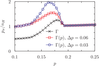
Figure 11: Ratio of the charge carrier concentrations as extracted from the conductivity ($p_{\sigma}$) and the Hall coefficient ($n_{H}$) as a function of doping. We chose $A_{p_{\text{min}}}=1.0$, where electron pockets exist for $0.13\leq p\leq 0.19$. $\Delta p$ is the doping range over which $\Gamma(p)$ doubles with decreasing doping.

In Fig. 10 we show results for the heat conductivity of a disordered antiferromagnetic metal as obtained with this choice of $\Gamma(p)$. We mentioned in the last sections that for $\Gamma(p)=\Gamma_{0}$ discrepancies between experiments and the theory of transport in a superconductor in the dirty limit showed up in the Hall angle and the doping dependence of the charge carrier density. In Fig. 11, we show the ratio between the charge carrier density as extracted from the conductivity and the Hall number. For $\Gamma(p)=\Gamma_{0}$, with decreasing doping we find a small peak and then a decrease to values significantly below one. Adding doping dependent scattering, the peak at $p<p^{\ast}$ increases as the conductivity drops faster. Note that in this section we assume that $R_{H}$ depends only weakly on the scattering rate for $\Gamma_{0}\ll E_{F}$, where $E_{F}$ is the Fermi energy. Our results for $p_{\sigma}/n_{H}$ can be compared with the experimental results by Collignon et al. Collignon et al. (2017), yielding good qualitative agreement.

A similar picture emerges from the Hall angle $R_{H}\sigma$. In Nd-LSCO, a drop by a factor of three is observed over the width of the transition with decreasing doping Collignon et al. (2017). In the disordered antiferromagnetic metal, a rather small drop is observed in this quantity for $p<p^{\ast}$, followed by an increase at smaller $p$. As can be seen in Fig. 12, adding doping dependent scattering allows to enhance the size of the drop and weakens the decrease at smaller doping, leading to a better qualitative agreement with the experimental results Collignon et al. (2017).

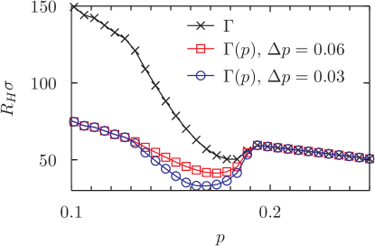
Figure 12: Hall angle as a function of doping computed for different doping-dependences of the scattering rate. We chose $A_{p_{\text{min}}}=1.0$, where electron pockets exist for $0.13\leq p\leq 0.19$. $\Delta p$ is the doping range over which $\Gamma(p)$ doubles with decreasing doping.

A doping-dependent scattering rate that increases for $p<p^{\ast}$ can thus improve the qualitative agreement between theory and experiment in various transport properties. In the following we argue that the competing ordering tendencies at different energy scales in underdoped cuprates could provide a mechanism for such a doping-dependence of the scattering rate. In La-based cuprates like Nd-LSCO, at low dopings ($p\sim 0.12$) there is evidence of stripe-like ordering from neutron scattering and X-ray spectroscopy Tranquada et al. (1995, 1996); Comin and Damascelli (2016). In other cuprate materials like BSCCO, local patches of charge modulations have been seen in STM experiments Fujita et al. (2014, 2014); Hamidian et al. (2016). Theoretical studies also show that the reconstructed small Fermi surface has a dominant instability towards bond-density waves (BDW) at an incommensurate wave-vector with a $d$-wave form factor Chowdhury and Sachdev (2014); Sachdev and Chowdhury (2016). The results of recent transport experiments Laliberte et al. (2016); Collignon et al. (2017) suggest that charge-ordering sets in at a lower doping than $p^{\ast}$, where the pseudogap line terminates. However, short-range charge density modulations seem to be omnipresent in the pseudogap phase, and could act as additional sources of scattering. Indeed, time-reversal symmetric disorder can destroy long range density wave order in the charge channel as it couples linearly to the order parameter, but it can only couple quadratically to the spin density wave order parameter and is therefore a less relevant perturbation to antiferromagnetic order Nie et al. (2017). Below, we explore a simple model of disordered density waves and estimate its contribution to the quasiparticle scattering rate.

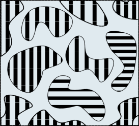
Figure 13: Patches of density waves that act as additional quenched disorder.

We model the disorder-induced scattering as arising from pinned short-range charge-density wave order with a domain size given by the correlation length $\xi$, which we assume to be of the order of ten lattice spacings. Each domain is locally unidirectional with an incommensurate ordering wave vectors ${\mathbf{Q}}$, as shown in Fig. 13. The order parameter $P_{ij}$ scatters an electron from momentum ${\mathbf{k}}-{\mathbf{Q}}/2$ to ${\mathbf{k}}+{\mathbf{Q}}/2$. Therefore, each such patch can be considered to be a short-range potential scatterer with the appropriate matrix element for scattering between electron states $\ket{{\mathbf{k}}}$ and $\ket{{\mathbf{k}}^{\prime}}$ being given by $P_{{\mathbf{Q}}}\,f\left[({\mathbf{k}}+{\mathbf{k}}^{\prime})/2\right]$, where $f({\mathbf{k}})$ is some appropriate internal form factor. We assume a phenomenological Lorentzian dependence on ${\mathbf{Q}}$ that it peaked at ${\mathbf{Q}}_{0}$, the ordering wave-vector with the largest susceptibility. Assuming weak disorder with a density $n_{i}\sim 0.01$, we can self-average over the disorder to find a scattering time $\tau_{2}$ given in the Born approximation by (assuming it is independent of initial state)

$$\tau_{2}^{-1} = 2\pi\int\frac{d^{2}{\mathbf{Q}}}{4\pi^{2}}g({\mathbf{Q}})\int\frac{d^{2}{\mathbf{k}}}{4\pi^{2}}\big{|}P_{{\mathbf{Q}}}({\mathbf{k}},{\mathbf{k}}^{\prime})f(({\mathbf{k}}+{\mathbf{k}}^{\prime})/2)\big{|}^{2}\delta(\xi_{{\mathbf{k}}}-\xi_{{\mathbf{k}}^{\prime}}),\text{ where }$$

$$P_{{\mathbf{Q}}}({\mathbf{k}},{\mathbf{k}}^{\prime}) \sim \frac{1}{\xi^{-2}+({\mathbf{k}}-{\mathbf{k}}^{\prime}-{\mathbf{Q}})^{2}},$$ (75)

where $g({\mathbf{Q}})$ is a normalized function peaked at ${\mathbf{Q}}_{0}$. Now a gradual increase in the density wave correlation length $\xi$ with decreasing doping can result in a larger scattering rate. Saturation of the charge-density wave correlation length due to disorder also entails saturation of the scattering rate.

VI Topological order in the pseudogap phase

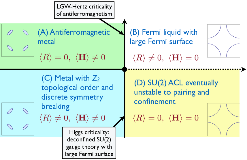
Figure 14: Phase diagram adapted from Refs. Sachdev and Chowdhury, 2016; Chatterjee and Sachdev, 2017. The $x$ and $y$ axes are parameters controlling the condensates of $\mathbf{H}$ and $R$ respectively. There is long-range antiferromagnetic order only in phase A, where both $R$ and $\mathbf{H}$ condensates are present. Phase C is a model for the pseudogap with topological order. We argue in the text that, in the simplest theory, the charge and energy transport properties of the A $\rightarrow$ B transition are identical to those of the C $\rightarrow$ D transition. The dashed line between phases C and D represents a crossover.

In this paper, we have so far discussed electrical and thermal transport in a mean-field model for a quantum phase transition from a (in-) commensurate antiferromagnet to a non-magnetic Fermi liquid. In Fig. 14, we present the phase diagram of a SU(2) lattice gauge theory Sachdev and Chowdhury (2016); Chatterjee and Sachdev (2017) of the square lattice Hubbard model, in which such a quantum transition corresponds to taking the route A $\rightarrow$ B with increasing doping. Along this route, the optimal doping criticality is associated with the Landau-Ginzburg-Wilson-Hertz Hertz (1976) theory of the antiferromagnetic quantum critical point. However, there have, so far, been no indications that long-range antiferromagnetic order is present in the pseudogap regime of the hole-doped cuprates. So we instead examine the route A $\rightarrow$ C $\rightarrow$ D $\rightarrow$ B in Fig. 14 as describing the evolution of phases with increasing hole-doping. In this route, the pseudogap is phase C, a metal with $\mathbb{Z}_{2}$ topological order, and the optical doping criticality is the topological phase transition between phases C and D.

The specific scenario illustrated in Fig. 14 assumes that the pseudogap is a $\mathbb{Z}_{2}$ algebraic charge liquid ($\mathbb{Z}_{2}$-ACL) or a $\mathbb{Z}_{2}$ fractionalized Fermi liquid ($\mathbb{Z}_{2}$-FL^∗) Sachdev and Chowdhury (2016); Sachdev et al. (2016). For both these phases, the only low energy quasiparticles are charge-carrying fermions with a small Fermi surface. These phases can be described as metals with quantum-fluctuating antiferromagnetism in the following manner. We introduce a spacetime-dependent SU(2) spin rotation, $R_{i}$ to transform the electron operators $c_{i\alpha}$ into ‘rotated’ fermions $\psi_{is}$, with $s=\pm$:

$$\left(\begin{array}[]{c}c_{i\uparrow}\\ c_{i\downarrow}\end{array}\right)=R_{i}\left(\begin{array}[]{c}\psi_{i,+}\\ \psi_{i,-}\end{array}\right),$$ (80)

where

$$R_{i}^{\dagger}R_{i}=R_{i}R_{i}^{\dagger}=1.$$ (81)

The same transformation rotates the local magnetization $\mathbf{m}_{i}$ to a ‘Higgs’ field $\mathbf{H}_{i}$

$${\bm{\sigma}}\cdot\mathbf{m}_{i}=R_{i}\,({\bm{\sigma}}\cdot\mathbf{H}_{i})\,R_{i}^{\dagger}$$ (82)

Note that under Eq. (82), the coupling of the magnetic moment $\mathbf{m}_{i}$ to the electrons is equal to the coupling of the Higgs field to the $\psi$ fermions

$$\mathbf{m}_{i}\cdot c_{i\alpha}^{\dagger}{\bm{\sigma}}_{\alpha\beta}c_{i\beta}^{\vphantom{\dagger}}=\mathbf{H}_{i}\cdot\psi_{is}^{\dagger}{\bm{\sigma}}_{ss^{\prime}}\psi_{is^{\prime}}^{\vphantom{\dagger}}$$ (83)

A second key observation is that the mappings in Eqs. (80) and (82) are invariant under the SU(2) gauge transformation generated by $V_{i}$, where

$$\left(\begin{array}[]{c}\psi_{i,+}\\ \psi_{i,-}\end{array}\right) \rightarrow V_{i}(\tau)\left(\begin{array}[]{c}\psi_{i,+}\\ \psi_{i,-}\end{array}\right)$$ (88)

$$\quad R_{i} \rightarrow R_{i} V_{i}^{\dagger}(\tau)$$

$${\bm{\sigma}}\cdot\mathbf{H}_{i} \rightarrow V_{i}\,({\bm{\sigma}}\cdot\mathbf{H}_{i})\,V_{i}^{\dagger}.$$ (89)

So the resulting theory for the $\psi$, $R$ and $\mathbf{H}$ will be a SU(2) lattice gauge theory.

We are interested here in the properties of state C as a model for the pseudogap. From Fig. 14, we observe that in this state the local antiferromagnetic order $\mathbf{m}_{i}$ quantum fluctuating, but the Higgs field (which is the antiferromagnetic order in a rotating reference frame) is a constant. Moreover, from Eq. (83), the coupling of the $\psi$ fermions to the Higgs field is identical to the coupling of the electrons to the physical magnetic moment. If we assume that the dispersions of the $\psi$ and $c$ fermions are the same (in a suitable gauge), then we can compute the charge and energy transport properties of the transition from state C to state D without further analysis: they are identical to the charge and energy transport properties of the transition from state A to state B which were computed in earlier sections of this paper. There are significant differences in the spin transport properties of C $\rightarrow$ D from A $\rightarrow$ B, but these have not so far been experimentally accessible in the cuprates.

So we have the important conclusion that the concurrence between theory and experiments, in this paper and in earlier work Storey (2016); Eberlein et al. (2016), applies also for the topological phase transition, C $\rightarrow$ D, model of the optical doping criticality. And this model has the important advantage that long-range antiferromagnetic order is not required in the pseudogap phase C. Phase D is described by a SU(2) gauge field coupled to a large Fermi surface of fermions with SU(2) gauge charges: such a phase is expected to be unstable to a superconductor in which all SU(2) gauge charges are confined, and so the state is formally the same as a BCS superconductor. However, a magnetic field could suppress the superconductivity and expose the underlying non-Fermi liquid, and this makes phase D a candidate to explain the observed strange metal in the overdoped regime Cooper et al. (2009).

We note that it is also possible to construct models of $\mathbb{Z}_{2}$-FL^∗, different from that in Fig. 14, building on the models reviewed in Ref. Lee et al., 2006 in which the low-energy charge-carrying excitations are bosonic Punk et al. (2015); Chatterjee et al. (2016). However, these models support charge-neutral spinons in the deconfined phase Chatterjee and Sachdev (2016) and therefore violate the Wiedemann-Franz law quite strongly. The reason is that the spinons contribute to the thermal conductivity but not to the electrical conductivity. Such violations have not been observed in experiments Grissonnanche et al. (2016).

VII Discussion

It is natural to ask how the presence of other excitations or fluctuations would affect our findings above. The parameter regime very close to the critical doping $p^{\ast}$ cannot be reliably described by our simple mean-field approach. This requires a more sophisticated theory of transport in a strange metal and the consideration of quantum critical fluctuations. However, the quantum critical regime of doping shrinks to a point as $T\rightarrow 0$, and away from this regime fermionic quasiparticles exist and are well-described by nearly non-interacting fermions. Interaction effects can be taken into account by Fermi liquid corrections Durst and Lee (2000) to the conductivities. In principle, vertex corrections and Fermi liquid corrections may be different on the two sides of the phase transition. We argued that the results for the conductivities in the dirty limit can be well understood under the assumption that the Fermi velocity does not change across the optimal doping QCP. There is experimental evidence for certain cuprates like BSSCO that the Fermi velocity is roughly constant across $p^{*}$, although it does get renormalized to smaller values for lower doping Sebastian et al. (2011); Vishik et al. (2010). Our results are thus robust if the Fermi velocity in the calculation is interpreted as the measured Fermi velocity from experiments. Fermi liquid corrections should thus not change our conclusions substantially. Moreover, we studied the interaction of fermions with disorder only within a simple relaxation time approximation. We expect this to capture the qualitative features in the relevant limits. It would be interesting to determine the scattering time self-consistently, as gapping out parts of the Fermi surface may also influence the scattering time. This could be done in an unconstrained Hartree-Fock calculation similar to Ref. Chen et al., 2009.

On the overdoped side, there are no gapless excitations besides the fermions. In the scenario where static iAF order disappears at the QCP, in the overdoped regime $p>p^{\ast}$ magnons are gapped and do not contribute to the heat conductivity at low temperatures. On the overdoped side of the QCP from the topological metal to the normal metal, there are also no additional low energy excitations which could contribute to thermal transport. The reason is that in this scenario, the normal metal is a confined phase, where all additional excitations carrying $\mathbb{Z}_{2}$ gauge charge are confined and the gauge field is massive.

Similar arguments hold in the underdoped regime. In the $\mathbb{Z}_{2}$-ACL or $\mathbb{Z}_{2}$-FL^∗ with fermionic chargons, the charge-neutral spin-excitations as well as the visons (which are the $\mathbb{Z}_{2}$ gauge fluxes) yield additional contributions to the heat conductivity at finite temperature. However, these are suppressed at low temperatures because the spinons and visons are both gapped. In the scenario with static iAF order, magnons yield additional contributions to the heat conductivity, which vanish at zero temperature. The two scenarios could possibly be distinguished at finite temperature, where gapped gauge fields contribute differently from magnons. Note that no magnon contribution to the heat conductivity of $\mathrm{YBCO}$ is seen beyond the doping where long-range commensurate antiferromagnetic order at finite temperature disappears in the strongly underdoped regime Doiron-Leyraud et al. (2006). This could, however, also be a consequence of long-range incommensurate antiferromagnetic order only existing in the ground state Haug et al. (2010). We leave the study of this interesting problem for future work.

VIII Conclusions

We summarize the main findings of our numerical computations for the electrical and thermal conductivities, and their relationship to observations.

In Fig. 3, we showed the doping dependence of the thermal conductivity of metallic states in the presence of spiral antiferromagnetic order at low doping. The comparison of these results with the commensurate antiferromagneticsm case appears in Fig. 4. Although there is a difference between these cases, both sets of results show that the drop in the thermal conductivity $\kappa$ between large and small $p$ is smaller than that found for the Hall effect in Ref. Eberlein et al., 2016, as shown in Fig. 5. These results are at odds with the recent observations of Collignon et al. Collignon et al. (2017); Michon et al. (2017) who found the same drop in the carrier density in the thermal conductivity and the Hall effect.

Next we turned to corresponding computations in the presence of superconductivity. In Fig. 8, we plotted the evolution of thermal conductivity as a function of doping in the clean and dirty limits. In the clean limit, $\kappa$ shows markedly different behavior for commensurate and incommensurate antiferromagnetic order. The appearance of Néel order entails a gradual drop of $\kappa$ on the underdoped side ($p<p^{*}$), whereas advent of incommensurate spiral order results in a sharp drop by a factor of two, consistent with our analytical results. Figure 9 depicts how this sharp drop is smoothened out as a function of increasing disorder. We also noted that appearance of antiferromagnetism can be distinguished from other orders (like charge density wave Durst and Sachdev (2009)) co-existing with superconductivity by studying the evolution of the thermal conductivity across the quantum critical point.

We then discussed how a doping-dependent scattering rate, possibly due to quenched density fluctuations, affects the thermal conductivity in the disordered antiferromagnetic metal or the dirty superconductor. Figure 10 shows the evolution of $\kappa$ for different doping dependent scattering rates. A comparison of the carrier densities extracted from conductivity and the Hall effect appears in Fig. 11, and a plot of the Hall angle as a function of doping is shown in Fig. 12; both are in good qualitative agreement with recent experimental data of Collignon et al. and Michon et al. Collignon et al. (2017); Michon et al. (2017).

Finally, we presented an alternate description of the pseudogap phase as an exotic metal with $\mathbb{Z}_{2}$ topological order, but without long range antiferromagnetism. Figure 14 shows a phase diagram outlining the two distinct routes from a small Fermi surface in the pseudogap phase to a large Fermi surface on the overdoped side. We argued that in both cases, the electrical, Hall Storey (2016); Eberlein et al. (2016) and thermal conductivities exhibit identical evolution as a function of doping at low temperatures, and therefore the observations in Refs. Collignon et al., 2017; Michon et al., 2017 can be equally well explained by a phase transition from a regular Fermi liquid to a topological pseudogap phase.

Appendix A Néel ordered $d$-wave superconductor and the phenomenon of nodal collision

Figure 15: Local coordinate systems adapted to the nodes, defined about the four nodal collision point $(\pm\pi/2,\pm\pi/2)$. The blue portion is the reduced BZ used in our calculations.

We take a more careful look at the nodes of the general dispersion described in Eq. (63) for ${\mathbf{Q}}=(\pi,\pi)$, with a bare fermionic dispersion $\xi_{{\mathbf{k}}}$ that pertains to the band structure of the overdoped cuprates. To model this, we choose the nodes to lie along the diagonal likes $k_{x}=\pm k_{y}$ at a distance $k_{F}$ from the origin. We assume that the node ${\mathbf{K}}_{0}$ in the first quadrant of the BZ is separated from the $(\pi/2,\pi/2)$ point by a small distance $k_{o}$, following Ref. Durst and Sachdev, 2009. The precise criteria is that the node lies quite close the center of the positive quadrant of the BZ, and the distance $k_{o}=\pi/\sqrt{2}-k_{F}$ is much smaller than $k_{F}$. Within this approximation, we see the same phenomenon of nodal collision which gaps out the nodal quasiparticles of the $d$-wave superconductors, as described for charge density waves in Ref. Durst and Sachdev, 2009. The diagonally opposite nodes collide at the boundary of the reduced BZ beyond a certain critical value of the order parameter $A$ (which we determine below), and this renders the spectrum fully gapped. Since we are mainly interested in the low-energy excitations near the nodes, we choose local coordinate systems centered at $(\pm\pi/2,\pm\pi/2)$ adapted to each node, as shown in Fig. 15.

For any $A\neq 0$, it is evident that $E_{+,{\mathbf{k}}}\neq 0$ for any ${\mathbf{k}}$. The condition for $E_{-,{\mathbf{k}}}=0$ can be reduced by some algebra to

$$\left(A^{2}-\xi_{{\mathbf{k}}}\xi_{{\mathbf{k}}+{\mathbf{Q}}}-\Delta_{{\mathbf{k}}}\Delta_{{\mathbf{k}}+{\mathbf{Q}}}\right)^{2}+\left(\xi_{{\mathbf{k}}}\Delta_{{\mathbf{k}}+{\mathbf{Q}}}-\xi_{{\mathbf{k}}+{\mathbf{Q}}}\Delta_{{\mathbf{k}}}\right)^{2}=0$$ (90)

Defining a local coordinate system $(k_{1},k_{2})$ about each of the collision points as shown in Fig. 15, to linear order in the momenta we find

$$\xi_{{\mathbf{k}}}=v_{F}(k_{0}+k_{1}),\;\Delta_{{\mathbf{k}}}=v_{\Delta}k_{2},\;\xi_{{\mathbf{k}}+{\mathbf{Q}}}=-v_{F}(k_{1}-k_{0}),\;\Delta_{{\mathbf{k}}+{\mathbf{Q}}}=-v_{\Delta}k_{2}$$ (91)

where $v_{F}$ and $v_{\Delta}$ are the Fermi velocity and gap velocity, respectively, at any node (they are all identical due to the fourfold rotation symmetry). Substituting these in Eq. (90), we find that it reduces to

$$\left(A^{2}+v_{F}^{2}k_{1}^{2}+v_{\Delta}^{2}k_{2}^{2}-v_{F}^{2}k_{0}^{2}\right)^{2}+(2v_{F}v_{\Delta}k_{o})^{2}k_{2}^{2}=0.$$ (92)

Thus, the nodes are located at

$$(k_{1},k_{2})=\left(\pm\sqrt{k_{o}^{2}-A^{2}/v_{F}^{2}},0\right),$$ (93)

where the minus sign corresponds to the node within the reduced BZ, and the plus sign corresponds to the shadow node in the 2nd BZ. From this expression, it is obvious that no nodes exist for spiral order parameters $A$ beyond a critical value $A_{c}=v_{F}k_{o}$. One can visualize this as the node and the shadow note approaching each other and annihilating at $(k_{1},k_{2})=(0,0)$, resulting in a gap in the quasiparticle spectrum for $A\geq A_{c}$. Note that this nodal collision leads to a half-filled insulator.

Appendix B Derivation of thermal conductivity for co-existing Néel order and superconductivity in the clean limit

For ${\mathbf{Q}}=(\pi,\pi)$ we note that ${\mathbf{v}_{F}}({\mathbf{k}}+{\mathbf{Q}})\approx-{\mathbf{v}_{F}}({\mathbf{k}})$, up to O$(k_{0}^{2})$, and ${\mathbf{v}_{\Delta}}({\mathbf{k}}+{\mathbf{Q}})=-{\mathbf{v}_{\Delta}}({\mathbf{k}})$. The velocity matrix $\mathbf{V}_{{\mathbf{k}}}$ can hence be simplified to:

$$\mathbf{V}_{{\mathbf{k}}}=\begin{pmatrix}{\mathbf{v}}_{1{\mathbf{k}}}&0\\ 0&{\mathbf{v}}_{2{\mathbf{k}}}\end{pmatrix},\text{ where }{\mathbf{v}}_{1{\mathbf{k}}}={\mathbf{v}_{F}}({\mathbf{k}})\tau_{3}+{\mathbf{v}_{\Delta}}({\mathbf{k}})\tau_{1},\text{ and }{\mathbf{v}}_{2{\mathbf{k}}}=-{\mathbf{v}_{F}}({\mathbf{k}})\tau_{3}+{\mathbf{v}_{\Delta}}({\mathbf{k}})\tau_{1}$$

This allows to rewrite the trace in Eq. (68) in terms of $G_{den}$, defined in Eq. (LABEL:ImGR) (again, using labels 1 for ${\mathbf{k}}$ and 2 for ${\mathbf{k}}+{\mathbf{Q}}$) at each nodal collision point,

$$\text{Tr}\left[G_{R}^{\prime\prime}({\mathbf{k}},0)\mathbf{V}_{{\mathbf{k}}}G_{R}^{\prime\prime}({\mathbf{k}},0)\mathbf{V}_{{\mathbf{k}}}\right] = 2\Gamma^{2}\bigg{[}(A^{2}+\Gamma^{2}+\xi_{1}^{2}+\Delta_{1}^{2})^{2}+(A^{2}+\Gamma^{2}+\xi_{2}^{2}+\Delta_{2}^{2})^{2}\bigg{]}\left({\mathbf{v}_{F}}{\mathbf{v}_{F}}+{\mathbf{v}_{\Delta}}{\mathbf{v}_{\Delta}}\right)/G_{den}^{2}$$

$$-4A^{2}\Gamma^{2}\bigg{[}\left((\xi_{1}+\xi_{2})^{2}-(\Delta_{1}+\Delta_{2})^{2}\right)\bigg{]}\left({\mathbf{v}_{F}}{\mathbf{v}_{F}}-{\mathbf{v}_{\Delta}}{\mathbf{v}_{\Delta}}\right)/G_{den}^{2}$$

Defining a local coordinate system $(k_{1},k_{2})$ about each of the collision points as shown in Fig. 15, we linearize the different terms in the Hamiltonian:

$$\xi_{1}=v_{F}(k_{0}+k_{1}),\;\Delta_{1}=v_{\Delta}k_{2},\;\xi_{2}=-v_{F}(k_{1}-k_{0}),\;\Delta_{2}=-v_{\Delta}k_{2}$$ (96)

Note that the numerator in Eq. (LABEL:trEqn) is proportional to $\Gamma^{2}$, which goes to zero in the clean limit. Therefore, the most important contributions come from the region of $k$ space where the denominator also goes to zero. In the linearized approximation described above, we find that:

$$G_{den}=\left(A^{2}+v_{F}^{2}k_{1}^{2}+v_{\Delta}^{2}k_{2}^{2}-v_{F}^{2}k_{0}^{2}\right)^{2}+(2v_{F}v_{\Delta}k_{o})^{2}k_{2}^{2}+O(\Gamma_{o}^{2})$$ (97)

Therefore, one can see that $G_{den}=0$ in the clean limit, only when $k_{2}=0$ and $k_{1}^{2}=k_{o}^{2}-A^{2}/v_{F}^{2}$. Therefore, beyond a critical strength of the AF order amplitude, i.e, for $A>A_{c}=v_{F}k_{o}$, there is no solution. With regards to the spectrum, this corresponds to the scenario with gapped quasiparticles in the commensurate case, and therefore in the clean limit the conductivity is equal to zero at $T=0$. In the dirty limit when $\Gamma\gtrsim\Delta$, this is not the case as the disorder induced self-energy modifies quasiparticle spectral weights and closes the gap.

As $\Gamma_{0}^{2}\rightarrow 0$, the terms in O$(\Gamma_{0}^{4})$ in the integral can be safely neglected, and the terms proportional to $\Gamma_{0}^{2}$ can be replaced by their values at the point where the denominator vanishes, i.e, $k_{2}=0$ and $k_{1}^{2}=k_{0}^{2}-A^{2}/v_{F}^{2}$. Within this approximation, we obtain

$$\text{Tr}\left[G_{R}^{\prime\prime}({\mathbf{k}},0)\mathbf{V}_{{\mathbf{k}}}G_{R}^{\prime\prime}({\mathbf{k}},0)\mathbf{V}_{{\mathbf{k}}}\right] = \Gamma^{2}\frac{2A_{c}^{2}(A_{c}^{2}-A^{2})\left({\mathbf{v}_{F}}{\mathbf{v}_{F}}+{\mathbf{v}_{\Delta}}{\mathbf{v}_{\Delta}}\right)-A^{2}A_{c}^{2}\left({\mathbf{v}_{F}}{\mathbf{v}_{F}}-{\mathbf{v}_{\Delta}}{\mathbf{v}_{\Delta}}\right)}{[\Gamma^{2}A_{c}^{2}+f]^{2}},\text{ where }$$

$$f = \frac{\left(A^{2}+v_{F}^{2}k_{1}^{2}+v_{\Delta}^{2}k_{2}^{2}-A_{c}^{2}\right)^{2}}{4}+A_{c}^{2}v_{\Delta}^{2}k_{2}^{2}$$ (98)

In the following we evaluate the diagonal conductivity and pick the $i^{\text{th}}$ component of the velocities, $i\in\{x,y\}$. Since in the coordinate system chosen, ${\mathbf{v}_{F}}$ and ${\mathbf{v}_{\Delta}}$ are parallel to either $\hat{k}_{1}$ or $\hat{k}_{2}$, so we have:

$$2\left({\mathbf{v}_{F}}{\mathbf{v}_{F}}\pm{\mathbf{v}_{\Delta}}{\mathbf{v}_{\Delta}}\right)_{ii}=v_{F}^{2}\pm v_{\Delta}^{2}$$ (99)

Rescaling the momenta by defining $\tilde{q}_{1}=v_{F}k_{1}$ and $\tilde{q}_{2}=v_{\Delta}k_{2}$, and multiplying by a factor of four for the four pairs of nodal points in the BZ (every point has the same contribution), we obtain

$$\frac{\kappa_{ii}(\Omega\rightarrow 0,T)}{T} = \frac{k_{B}^{2}(v_{F}^{2}+v_{\Delta}^{2})}{3v_{F}v_{\Delta}}\int\frac{d^{2}\tilde{q}}{2\pi}\frac{\Gamma^{2}A_{c}^{2}(A_{c}^{2}-A^{2}/2)}{\left(\Gamma^{2}A_{c}^{2}+\left(A^{2}+\tilde{q}^{2}-A_{c}^{2}\right)^{2}/4+A_{c}^{2}\tilde{q}_{2}^{2}\right)^{2}}$$ (100)

$$-\frac{k_{B}^{2}(v_{F}^{2}-v_{\Delta}^{2})}{3v_{F}v_{\Delta}}\int\frac{d^{2}\tilde{q}}{2\pi}\frac{\Gamma^{2}A_{c}^{2}A^{2}/2}{\left(\Gamma^{2}A_{c}^{2}+\left(A^{2}+\tilde{q}^{2}-A_{c}^{2}\right)^{2}/4+A_{c}^{2}\tilde{q}_{2}^{2}\right)^{2}}$$

for the diagonal conductivity. The integrals in Eq. (100) can be analytically evaluated in the clean limit. We first cast the integrals in terms of dimensionless variables $\gamma=\Gamma_{o}/A_{c}$, $q_{i}=\tilde{q}_{i}/A_{c}$ and $\alpha=A/A_{c}$, measuring energy in units of $A_{c}=k_{0}v_{F}$.

$$I_{1} = \left(1-\frac{\alpha^{2}}{2}\right)\int\frac{d^{2}q}{2\pi}\frac{\gamma^{2}}{\left(\gamma^{2}+\left(1+q^{2}-\alpha^{2}\right)^{2}/4+q_{2}^{2}\right)^{2}}\equiv\left(1-\frac{\alpha^{2}}{2}\right)I_{3}$$

$$I_{2} = \frac{\alpha^{2}}{2}\int\frac{d^{2}q}{2\pi}\frac{\gamma^{2}}{\left(\gamma^{2}+\left(1+q^{2}-\alpha^{2}\right)^{2}/4+q_{2}^{2}\right)^{2}}\equiv\frac{\alpha^{2}}{2}I_{3}$$ (101)

Now we change variables to $q_{1}=1+x\cos\theta$, and $q_{2}=x\text{ sin }\theta$. Then the denominator of the integral can be written as:

$$\gamma^{2}+\left(1+q^{2}-\alpha^{2}\right)^{2}/4+q_{2}^{2} = \gamma^{2}+x^{2}+\left(\frac{x^{2}+\alpha^{2}}{2}\right)^{2}+x(x^{2}+\alpha^{2})\cos\theta$$

$$= \left(\tilde{\gamma}^{2}+1+h^{2}+2h\cos\theta\right)x^{2},\text{ where }\tilde{\gamma}=\gamma/x,h=\frac{x^{2}+\alpha^{2}}{2x}$$

Plugging this back into the integral and shifting $\theta\rightarrow\theta+\pi$, we find:

$$I_{3} = \int_{0}^{\infty}\frac{dx\,x}{2\pi}\int_{-\pi}^{\pi}d\theta\frac{\tilde{\gamma}^{2}x^{2}}{x^{4}\left(\tilde{\gamma}^{2}+1+h^{2}-2h\cos\theta\right)^{2}}$$ (103)

$$= \int_{0}^{\infty}\frac{dx\,x}{\pi}\int_{0}^{\pi}d\theta\frac{\tilde{\gamma}^{2}x^{2}}{x^{4}\left(\tilde{\gamma}^{2}+1+h^{2}-2h\cos\theta\right)^{2}}$$

$$= \int_{0}^{\infty}\frac{dx}{\pi x}I_{4}$$

where

$$I_{4} \equiv \int_{0}^{\pi}d\theta\frac{\tilde{\gamma}^{2}}{\left(\tilde{\gamma}^{2}+1+h^{2}-2h\cos\theta\right)^{2}}$$ (104)

$$= \frac{2\pi(1+h^{2})}{(1+h)^{3}}D(h-1,\tilde{\gamma}^{2}),\text{ with }D(u,v)\equiv\frac{v^{2}/2}{(u^{2}+v^{2})^{3/2}}$$

where we have already used $\tilde{\gamma}\rightarrow 0$ to simplify the integral. Note that $D(u,v)$ vanishes in the limit of $v\rightarrow 0$ for all $u$ expect $u=0$, where it diverges. Moreover, it also satisfies:

$$\int_{-\infty}^{\infty}duD(u,v)=1$$ (105)

Therefore, in the $\Gamma_{o}\rightarrow 0$ limit, which also corresponds to the second argument $\tilde{\gamma}^{2}\rightarrow 0$, we can replace $D(h-1,\tilde{\gamma}^{2})$ by $\delta(h-1)$. In this limit, we have:

$$I_{4}=\frac{2\pi(1+h^{2})}{(1+h)^{3}}D(h-1,\tilde{\gamma}^{2})\;\overset{\tilde{\gamma}^{2}\rightarrow 0}{\longrightarrow}\;\frac{\pi}{2}\,\delta(h-1)$$ (106)

Finally, we can plug back $I_{4}$ into $I_{3}$ and evaluate the sum over the delta-function:

$$I_{3} = \int_{0}^{\infty}\frac{dx}{\pi x}\;\frac{\pi}{2}\,\delta\left(\frac{x^{2}+\alpha^{2}}{2x}-1\right)$$ (107)

$$= \frac{1}{2}\int_{0}^{\infty}dx\left[\frac{\delta(x-x_{+})}{\sqrt{1-\alpha^{2}}}+\frac{\delta(x-x_{-})}{\sqrt{1-\alpha^{2}}}\right],\text{ where }x_{\pm}=1\pm\sqrt{1-\alpha^{2}}$$

$$= \frac{1}{\sqrt{1-\alpha^{2}}}\;\text{ provided }\alpha<1,\text{ and }0\text{ otherwise}$$

Putting all of this together, we arrive at the finite expression of the static diagonal thermal conductivity in the clean limit for coexisting Néel order and superconductivity:

$$\frac{\kappa_{ii}(\Omega\rightarrow 0,T)}{T}=\frac{k_{B}^{2}}{3v_{F}v_{\Delta}}\bigg{[}\sqrt{1-\alpha^{2}}\,v_{F}^{2}+\frac{1}{\sqrt{1-\alpha^{2}}}v_{\Delta}^{2}\bigg{]}\Theta(1-\alpha),\text{ where }\alpha=\frac{A}{A_{c}}$$ (108)

Appendix C Particle-particle bubble in spiral antiferromagnet or algebraic charge liquid

In this paper, as well as in Refs. Yamase et al. (2016); Sushkov and Kotov (2004), it was assumed that Cooper pairs in a spiral antiferromagnetic state have vanishing total momentum. In order to substantiate this assumption, we compute the particle-particle bubble in a spiral state. Its momentum dependence at vanishing bosonic frequency is given by

$$L_{\text{PP}}(\boldsymbol{q})= -\int\frac{d^{3}k}{(2\pi)^{3}}\Bigl{\{}f(\boldsymbol{k}+\tfrac{\boldsymbol{q}}{2})^{2}G_{++}(k_{0},\boldsymbol{k})G_{--}(-k_{0},\boldsymbol{k}+\boldsymbol{Q})$$ (109)

$$+f(\boldsymbol{k}+\tfrac{\boldsymbol{q}}{2})f(\boldsymbol{k}+\boldsymbol{Q}+\tfrac{\boldsymbol{q}}{2})G_{+-}(k_{0},\boldsymbol{k})G_{-+}(-k_{0},\boldsymbol{k}+\boldsymbol{Q})\Bigr{\}}.$$

where $G_{ij}$ are the components of Eq. (33). This result can be rewritten as

$$= -\int\frac{d^{3}k}{(2\pi)^{3}}\Bigl{\{}f(\boldsymbol{k}+\tfrac{\boldsymbol{q}}{2})^{2}G_{++}(k_{0},\boldsymbol{k})G_{++}(k_{0},\boldsymbol{k})^{\ast}$$ (110)

$$+f(\boldsymbol{k}+\tfrac{\boldsymbol{q}}{2})f(\boldsymbol{k}+\boldsymbol{Q}+\tfrac{\boldsymbol{q}}{2})G_{+-}(k_{0},\boldsymbol{k})G_{+-}(k_{0},\boldsymbol{k})^{\ast}\Bigr{\}}$$

by exploiting the definition of the components of the propagator. Evaluation of the frequency integral yields

$$\begin{split}=&-\int\frac{d^{2}k}{(2\pi)^{2}}\sum_{i=\pm,j=\pm}\epsilon_{i}\epsilon_{j}\frac{1-n_{F}(E_{\boldsymbol{k}+\boldsymbol{q},i})-n_{F}(E_{\boldsymbol{k},j})}{(E_{\boldsymbol{k}+\boldsymbol{q},i}+E_{\boldsymbol{k},j})(E_{\boldsymbol{k}+\boldsymbol{q},+}-E_{\boldsymbol{k}+\boldsymbol{q},-})(E_{\boldsymbol{k},+}-E_{\boldsymbol{k},-})}\\ &\times\Bigl{\{}f(\boldsymbol{k}+\tfrac{\boldsymbol{q}}{2})^{2}(E_{\boldsymbol{k}+\boldsymbol{q},i}-\xi_{\boldsymbol{k}+\boldsymbol{q}+\boldsymbol{Q}})(E_{\boldsymbol{k},j}-\xi_{\boldsymbol{k}+\boldsymbol{Q}})+f(\boldsymbol{k}+\tfrac{\boldsymbol{q}}{2})f(\boldsymbol{k}+\boldsymbol{Q}+\tfrac{\boldsymbol{q}}{2})A^{2}\Bigr{\}}\end{split}$$ (111)

where $\epsilon_{\pm}=\pm 1$. In Fig. 16 we show numerical results for the particle-particle bubble in the $d$-wave channel. It is very strongly peaked at $\boldsymbol{q}=0$, as assumed in Refs. Yamase et al., 2016; Sushkov and Kotov, 2004. This is already suggested by the functional form of $L_{\text{PP}}(\boldsymbol{q})$ when written as in Eq. (110). The momentum dependence does not possess a four-fold rotation symmetry, as expected in a spiral state.

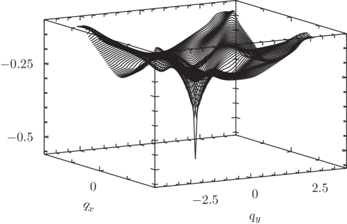
Figure 16: Momentum dependence of the $d$-wave particle-particle bubble for $t^{\prime}=-0.35$, $A=0.51$, $\eta=0.08$ and $p=0.09$.

References

- Badoux et al. (2016) S. Badoux, W. Tabis, F. Laliberté, G. Grissonnanche, B. Vignolle, D. Vignolles, J. Béard, D. A. Bonn, W. N. Hardy, R. Liang, N. Doiron-Leyraud, L. Taillefer, and C. Proust, “Change of carrier density at the pseudogap critical point of a cuprate superconductor,” Nature 531, 210 (2016), arXiv:1511.08162 [cond-mat.supr-con] .
- Laliberte et al. (2016) F. Laliberte, W. Tabis, S. Badoux, B. Vignolle, D. Destraz, N. Momono, T. Kurosawa, K. Yamada, H. Takagi, N. Doiron-Leyraud, C. Proust, and L. Taillefer, “Origin of the metal-to-insulator crossover in cuprate superconductors,” ArXiv e-prints (2016), arXiv:1606.04491 [cond-mat.supr-con] .
- Collignon et al. (2017) C. Collignon, S. Badoux, S. A. A. Afshar, B. Michon, F. Laliberté, O. Cyr-Choinière, J.-S. Zhou, S. Licciardello, S. Wiedmann, N. Doiron-Leyraud, and L. Taillefer, “Fermi-surface transformation across the pseudogap critical point of the cuprate superconductor ,” Phys. Rev. B 95, 224517 (2017), arXiv:1607.05693 [cond-mat.supr-con] .
- Michon et al. (2017) B. M. Michon, S. Li, P. Bourgeois-Hope, S. Badoux, J.-S. Zhou, N. Doiron-Leyraud, and L. Taillefer, “Pseudogap critical point inside the superconducting phase of a cuprate : a thermal conductivity study in nd-lsco,” in preparation (2017).
- Storey (2016) J. G. Storey, “Hall effect and Fermi surface reconstruction via electron pockets in the high- cuprates,” Europhys. Lett. 113, 27003 (2016), arXiv:1512.03112 [cond-mat.supr-con] .
- Eberlein et al. (2016) A. Eberlein, W. Metzner, S. Sachdev, and H. Yamase, “Fermi surface reconstruction and drop in the Hall number due to spiral antiferromagnetism in high- cuprates,” Phys. Rev. Lett. 117, 187001 (2016), arXiv:1607.06087 [cond-mat.str-el] .
- Sharma et al. (2017) G. Sharma, S. Nandy, A. Taraphder, and S. Tewari, “Suppression of hall number due to charge density wave order in high- cuprates,” arXiv preprint arXiv:1703.04620 (2017).
- Yang et al. (2006) K.-Y. Yang, T. M. Rice, and F.-C. Zhang, “Phenomenological theory of the pseudogap state,” Phys. Rev. B 73, 174501 (2006), arXiv:cond-mat/0602164 [cond-mat.supr-con] .
- Kaul et al. (2007) R. K. Kaul, A. Kolezhuk, M. Levin, S. Sachdev, and T. Senthil, “Hole dynamics in an antiferromagnet across a deconfined quantum critical point,” Phys. Rev. B 75, 235122 (2007), cond-mat/0702119 .
- Qi and Sachdev (2010) Y. Qi and S. Sachdev, “Effective theory of Fermi pockets in fluctuating antiferromagnets,” Phys. Rev. B 81, 115129 (2010), arXiv:0912.0943 [cond-mat.str-el] .
- Sachdev and Chowdhury (2016) S. Sachdev and D. Chowdhury, “The novel metallic states of the cuprates: Fermi liquids with topological order and strange metals,” Progress of Theoretical and Experimental Physics 2016, 12C102 (2016), arXiv:1605.03579 [cond-mat.str-el] .
- Chatterjee and Sachdev (2016) S. Chatterjee and S. Sachdev, “Fractionalized fermi liquid with bosonic chargons as a candidate for the pseudogap metal,” Phys. Rev. B 94, 205117 (2016), arXiv:1607.05727 [cond-mat.str-el] .
- Caprara et al. (2016) S. Caprara, C. Di Castro, G. Seibold, and M. Grilli, “Dynamical charge density waves rule the phase diagram of cuprates,” ArXiv e-prints (2016), arXiv:1604.07852 [cond-mat.supr-con] .
- Wu et al. (2011) T. Wu, H. Mayaffre, S. Kramer, M. Horvatic, C. Berthier, W. N. Hardy, R. Liang, D. A. Bonn, and M.-H. Julien, “Magnetic-field-induced charge-stripe order in the high-temperature superconductor ,” Nature 477, 191 (2011), arXiv:1109.2011 [cond-mat.supr-con] .
- Wu et al. (2013) T. Wu, H. Mayaffre, S. Krämer, M. Horvatić, C. Berthier, P. L. Kuhns, A. P. Reyes, R. Liang, W. N. Hardy, D. A. Bonn, and M.-H. Julien, “Emergence of charge order from the vortex state of a high-temperature superconductor,” Nat Commun 4, 2113 (2013), arXiv:1307.2049 [cond-mat.supr-con] .
- LeBoeuf et al. (2013) D. LeBoeuf, S. Kramer, W. N. Hardy, R. Liang, D. A. Bonn, and C. Proust, “Thermodynamic phase diagram of static charge order in underdoped ,” Nat Phys 9, 79 (2013), arXiv:1211.2724 [cond-mat.supr-con] .
- Gerber et al. (2015) S. Gerber, H. Jang, H. Nojiri, S. Matsuzawa, H. Yasumura, D. A. Bonn, R. Liang, W. N. Hardy, Z. Islam, A. Mehta, S. Song, M. Sikorski, D. Stefanescu, Y. Feng, S. A. Kivelson, T. P. Devereaux, Z.-X. Shen, C.-C. Kao, W.-S. Lee, D. Zhu, and J.-S. Lee, “Three-dimensional charge density wave order in at high magnetic fields,” Science 350, 949 (2015), arXiv:1506.07910 [cond-mat.str-el] .
- Doiron-Leyraud et al. (2007) N. Doiron-Leyraud, C. Proust, D. LeBoeuf, J. Levallois, J.-B. Bonnemaison, R. Liang, D. A. Bonn, W. N. Hardy, and L. Taillefer, “Quantum oscillations and the Fermi surface in an underdoped high-Tc superconductor,” Nature 447, 565 (2007), arXiv:0801.1281 [cond-mat.supr-con] .
- LeBoeuf et al. (2007) D. LeBoeuf, N. Doiron-Leyraud, J. Levallois, R. Daou, J.-B. Bonnemaison, N. E. Hussey, L. Balicas, B. J. Ramshaw, R. Liang, D. A. Bonn, W. N. Hardy, S. Adachi, C. Proust, and L. Taillefer, “Electron pockets in the fermi surface of hole-doped high-tc superconductors,” Nature 450, 533 (2007), arXiv:0806.4621 [cond-mat.supr-con] .
- Kemper et al. (2016) J. B. Kemper, O. Vafek, J. B. Betts, F. F. Balakirev, W. N. Hardy, R. Liang, D. A. Bonn, and G. S. Boebinger, “Thermodynamic signature of a magnetic-field-driven phase transition within the superconducting state of an underdoped cuprate,” Nat Phys 12, 47 (2016), arXiv:1403.3702 [cond-mat.supr-con] .
- Chan et al. (2016) M. K. Chan, N. Harrison, R. D. McDonald, B. J. Ramshaw, K. A. Modic, N. Barisic, N., and M. Greven, “Single reconstructed fermi surface pocket in an underdoped single-layer cuprate superconductor,” Nature Communications 7, 12244 (2016).
- Durst and Lee (2000) A. C. Durst and P. A. Lee, “Impurity-induced quasiparticle transport and universal-limit wiedemann-franz violation in d-wave superconductors,” Phys. Rev. B 62, 1270 (2000), arXiv:cond-mat/9908182 .
- Sushkov and Kotov (2004) O. P. Sushkov and V. N. Kotov, “Superconducting spiral phase in the two-dimensional model,” Phys. Rev. B 70, 024503 (2004), arXiv:cond-mat/0310635 .
- Yamase et al. (2016) H. Yamase, A. Eberlein, and W. Metzner, “Coexistence of incommensurate magnetism and superconductivity in the two-dimensional Hubbard model,” Phys. Rev. Lett. 116, 096402 (2016), arXiv:1507.00560 [cond-mat.str-el] .
- Durst and Sachdev (2009) A. C. Durst and S. Sachdev, “Low-temperature quasiparticle transport in a -wave superconductor with coexisting charge order,” Phys. Rev. B 80, 054518 (2009), arXiv:0810.3914 [cond-mat.supr-con] .
- Voruganti et al. (1992) P. Voruganti, A. Golubentsev, and S. John, “Conductivity and hall effect in the two-dimensional hubbard model,” Phys. Rev. B 45, 13945 (1992).
- Ambegaokar and Griffin (1965) V. Ambegaokar and A. Griffin, “Theory of the thermal conductivity of superconducting alloys with paramagnetic impurities,” Phys. Rev. 137, A1151 (1965).
- Schulz (1990) H. J. Schulz, “Incommensurate antiferromagnetism in the two-dimensional Hubbard model,” Phys. Rev. Lett. 64, 1445 (1990).
- Halboth and Metzner (2000) C. J. Halboth and W. Metzner, “-wave superconductivity and Pomeranchuk instability in the two-dimensional Hubbard model,” Phys. Rev. Lett. 85, 5162 (2000).
- Maier et al. (2000) T. Maier, M. Jarrell, T. Pruschke, and J. Keller, “-wave superconductivity in the hubbard model,” Phys. Rev. Lett. 85, 1524 (2000).
- Lichtenstein and Katsnelson (2000) A. I. Lichtenstein and M. I. Katsnelson, “Antiferromagnetism and d-wave superconductivity in cuprates: A cluster dynamical mean-field theory,” Phys. Rev. B 62, R9283 (2000).
- Maier et al. (2005) T. A. Maier, M. Jarrell, T. C. Schulthess, P. R. C. Kent, and J. B. White, “Systematic study of -wave superconductivity in the 2d repulsive hubbard model,” Phys. Rev. Lett. 95, 237001 (2005).
- Capone and Kotliar (2006) M. Capone and G. Kotliar, “Competition between -wave superconductivity and antiferromagnetism in the two-dimensional hubbard model,” Phys. Rev. B 74, 054513 (2006).
- Aichhorn et al. (2006) M. Aichhorn, E. Arrigoni, M. Potthoff, and W. Hanke, “Antiferromagnetic to superconducting phase transition in the hole- and electron-doped hubbard model at zero temperature,” Phys. Rev. B 74, 024508 (2006).
- Khatami et al. (2008) E. Khatami, A. Macridin, and M. Jarrell, “Effect of long-range hopping on in a two-dimensional hubbard-holstein model of the cuprates,” Phys. Rev. B 78, 060502 (2008).
- Kancharla et al. (2008) S. S. Kancharla, B. Kyung, D. Sénéchal, M. Civelli, M. Capone, G. Kotliar, and A.-M. S. Tremblay, “Anomalous superconductivity and its competition with antiferromagnetism in doped Mott insulators,” Phys. Rev. B 77, 184516 (2008).
- Friederich et al. (2011) S. Friederich, H. C. Krahl, and C. Wetterich, “Functional renormalization for spontaneous symmetry breaking in the Hubbard model,” Phys. Rev. B 83, 155125 (2011).
- Gull et al. (2013) E. Gull, O. Parcollet, and A. J. Millis, “Superconductivity and the pseudogap in the two-dimensional hubbard model,” Phys. Rev. Lett. 110, 216405 (2013).
- Eberlein and Metzner (2014) A. Eberlein and W. Metzner, “Superconductivity in the two-dimensional --Hubbard model,” Phys. Rev. B 89, 035126 (2014), arXiv:1308.4845 [cond-mat.str-el] .
- Rømer et al. (2016) A. T. Rømer, I. Eremin, P. J. Hirschfeld, and B. M. Andersen, “Superconducting phase diagram of itinerant antiferromagnets,” Phys. Rev. B 93, 174519 (2016), arXiv:1505.03003 [cond-mat.supr-con] .
- Zheng and Chan (2016) B.-X. Zheng and G. K.-L. Chan, “Ground-state phase diagram of the square lattice hubbard model from density matrix embedding theory,” Phys. Rev. B 93, 035126 (2016), arXiv:1504.01784 [cond-mat.str-el] .
- Hamidian et al. (2016) M. H. Hamidian, S. D. Edkins, C. K. Kim, J. C. Davis, A. P. MacKenzie, H. Eisaki, S. Uchida, M. J. Lawler, E.-A. Kim, S. Sachdev, and K. Fujita, “Atomic-scale electronic structure of the cuprate d-symmetry form factor density wave state,” Nature Physics 12, 150 (2016), arXiv:1507.07865 [cond-mat.supr-con] .
- Sarkar et al. (2017) T. Sarkar, P. Mandal, J. Higgins, Y. Zhao, H. Yu, K. Jin, and R. L. Greene, “Fermi surface reconstruction and anomalous low temperature resistivity in electron-doped la2-xcexcuo4,” ArXiv e-prints (2017), arXiv:1706.07836 .
- Tranquada et al. (1995) J. Tranquada, B. Sternlieb, J. Axe, Y. Nakamura, and S. Uchida, “Evidence for stripe correlations of spins and holes in copper oxide superconductors,” Nature 375, 561 (1995).
- Tranquada et al. (1996) J. M. Tranquada, J. D. Axe, N. Ichikawa, Y. Nakamura, S. Uchida, and B. Nachumi, “Neutron-scattering study of stripe-phase order of holes and spins in ,” Phys. Rev. B 54, 7489 (1996).
- Comin and Damascelli (2016) R. Comin and A. Damascelli, “Resonant x-ray scattering studies of charge order in cuprates,” Annual Review of Condensed Matter Physics 7, 369 (2016).
- Fujita et al. (2014) K. Fujita, M. H. Hamidian, S. D. Edkins, C. K. Kim, Y. Kohsaka, M. Azuma, M. Takano, H. Takagi, H. Eisaki, S.-i. Uchida, A. Allais, M. J. Lawler, E.-A. Kim, S. Sachdev, and J. C. S. Davis, “Direct phase-sensitive identification of a d-form factor density wave in underdoped cuprates,” Proceedings of the National Academy of Sciences 111, E3026 (2014).
- Fujita et al. (2014) K. Fujita, C. K. Kim, I. Lee, J. Lee, M. H. Hamidian, I. A. Firmo, S. Mukhopadhyay, H. Eisaki, S. Uchida, M. J. Lawler, E.-A. Kim, and J. C. Davis, “Simultaneous Transitions in Cuprate Momentum-Space Topology and Electronic Symmetry Breaking,” Science 344, 612 (2014), arXiv:1403.7788 [cond-mat.supr-con] .
- Chowdhury and Sachdev (2014) D. Chowdhury and S. Sachdev, “Density-wave instabilities of fractionalized Fermi liquids,” Phys. Rev. B 90, 245136 (2014), arXiv:1409.5430 [cond-mat.str-el] .
- Nie et al. (2017) L. Nie, A. V. Maharaj, E. Fradkin, and S. A. Kivelson, “Vestigial nematicity from spin and/or charge order in the cuprates,” arXiv preprint arXiv:1701.02751 (2017).
- Chatterjee and Sachdev (2017) S. Chatterjee and S. Sachdev, “Insulators and metals with topological order and discrete symmetry breaking,” Phys. Rev. B 95, 205133 (2017), arXiv:1703.00014 [cond-mat.str-el] .
- Hertz (1976) J. A. Hertz, “Quantum critical phenomena,” Phys. Rev. B 14, 1165 (1976).
- Sachdev et al. (2016) S. Sachdev, E. Berg, S. Chatterjee, and Y. Schattner, “Spin density wave order, topological order, and fermi surface reconstruction,” Phys. Rev. B 94, 115147 (2016).
- Cooper et al. (2009) R. A. Cooper, Y. Wang, B. Vignolle, O. J. Lipscombe, S. M. Hayden, Y. Tanabe, T. Adachi, Y. Koike, M. Nohara, H. Takagi, C. Proust, and N. E. Hussey, “Anomalous Criticality in the Electrical Resistivity of La2-xSrxCuO4,” Science 323, 603 (2009).
- Lee et al. (2006) P. A. Lee, N. Nagaosa, and X.-G. Wen, “Doping a Mott insulator: Physics of high-temperature superconductivity,” Rev. Mod. Phys. 78, 17 (2006), arXiv:cond-mat/0410445 .
- Punk et al. (2015) M. Punk, A. Allais, and S. Sachdev, “A quantum dimer model for the pseudogap metal,” Proc. Nat. Acad. Sci. 112, 9552 (2015), arXiv:1501.00978 [cond-mat.str-el] .
- Chatterjee et al. (2016) S. Chatterjee, Y. Qi, S. Sachdev, and J. Steinberg, “Superconductivity from a confinement transition out of a fractionalized Fermi liquid with topological and Ising-nematic orders,” Phys. Rev. B 94, 024502 (2016), arXiv:1603.03041 [cond-mat.str-el] .
- Grissonnanche et al. (2016) G. Grissonnanche, F. Laliberté, S. Dufour-Beauséjour, M. Matusiak, S. Badoux, F. F. Tafti, B. Michon, A. Riopel, O. Cyr-Choinière, J. C. Baglo, B. J. Ramshaw, R. Liang, D. A. Bonn, W. N. Hardy, S. Krämer, D. LeBoeuf, D. Graf, N. Doiron-Leyraud, and L. Taillefer, “Wiedemann-franz law in the underdoped cuprate superconductor ,” Phys. Rev. B 93, 064513 (2016).
- Sebastian et al. (2011) S. E. Sebastian, N. Harrison, and G. G. Lonzarich, “Quantum oscillations in the high-tc cuprates,” Philosophical Transactions of the Royal Society of London A: Mathematical, Physical and Engineering Sciences 369, 1687 (2011), http://rsta.royalsocietypublishing.org/content/369/1941/1687.full.pdf .
- Vishik et al. (2010) I. M. Vishik, W. S. Lee, R.-H. He, M. Hashimoto, Z. Hussain, T. P. Devereaux, and Z.-X. Shen, “Arpes studies of cuprate fermiology: superconductivity, pseudogap and quasiparticle dynamics,” New Journal of Physics 12, 105008 (2010).
- Chen et al. (2009) W. Chen, B. M. Andersen, and P. J. Hirschfeld, “Theory of resistivity upturns in metallic cuprates,” Phys. Rev. B 80, 134518 (2009).
- Doiron-Leyraud et al. (2006) N. Doiron-Leyraud, M. Sutherland, S. Y. Li, L. Taillefer, R. Liang, D. A. Bonn, and W. N. Hardy, “Onset of a boson mode at the superconducting critical point of underdoped ,” Phys. Rev. Lett. 97, 207001 (2006), cond-mat/0606645 .
- Haug et al. (2010) D. Haug, V. Hinkov, Y. Sidis, P. Bourges, N. B. Christensen, A. Ivanov, T. Keller, C. T. Lin, and B. Keimer, “Neutron scattering study of the magnetic phase diagram of underdoped ,” New J. Phys. 12, 105006 (2010), arXiv:1008.4298 [cond-mat.str-el] .