Maxi-sizing the trilinear Higgs self-coupling: how large could it be?

Abstract

In order to answer the question on how much the trilinear Higgs self-coupling could deviate from its Standard Model value in weakly coupled models, we study both theoretical and phenomenological constraints. As a first step, we discuss this question by modifying the Standard Model using effective operators. Considering constraints from vacuum stability and perturbativity, we show that only the latter can be reliably assessed in a model-independent way. We then focus on UV models which receive constraints from Higgs coupling measurements, electroweak precision tests, vacuum stability and perturbativity. We find that the interplay of current measurements with perturbativity already exclude self-coupling modifications above a factor of few with respect to the Standard Model value.

1 Introduction

The recent discovery of the Higgs boson at the Large Hadron Collider (LHC) [1, 2] marks a milestone event for high-energy physics. Yet, the Higgs boson is only a remnant of the underlying mechanism of spontaneous electroweak (EW) symmetry breaking, the so-called Brout-Englert-Higgs mechanism [3, 4]. In order to improve our understanding of the dynamics initiating EW symmetry breaking, a key ingredient is the global structure of the scalar potential that triggers the spontaneous breaking of $SU(2)_{L}\times U(1)_{Y}\to U(1)_{\mathrm{QED}}$. While the ongoing LHC program, focusing on precise measurements of Higgs and gauge boson masses and couplings, will continue to improve our understanding of the potential’s local structure in the vicinity of the EW minimum, information on the shape of the vacuum in a model-independent way is experimentally very difficult to obtain.

However, if one specifies the degrees of freedom and interactions in the scalar sector, one can calculate the form of the scalar potential. After EW symmetry breaking such potential gives rise to multi-scalar interactions, i.e. at lowest order cubic and quartic Higgs self-interactions. While the former can be probed directly in searches for multi-Higgs final states [7, 8, 9, 10, 11, 12, 13, 14, 15, 16, 17, 18, 19, 20, 21, 22, 23, 24, 25, 26, 27, 28, 29], indirectly via their effect on precision observables [30, 31] or loop corrections to single Higgs production [32, 33, 34, 35, 36], the latter are inaccessible at the LHC or a future linear collider [37, 38, 39]. Thus, to obtain a glimpse at the shape of the scalar potential we have to focus on the cubic scalar self-coupling.

If new light degrees of freedom contribute to the Higgs potential, they typically dominate the multi-Higgs phenomenology. On the other hand, if new degrees of freedom are heavy, it is widely argued that the Effective Field Theory (EFT) approach is most suitable to study deformations of the Standard Model (SM) Higgs potential in a rather model-independent and predictive way. Thus, in the latter case, where we assume that no light states below the cutoff scale $\Lambda\gg v\equiv 246$ GeV exist, it is tempting to introduce an operator $|H|^{6}$ (where $H$ denotes the usual Higgs doublet) and connect the (global) properties of the vacuum, e.g. whether the EW minimum is a local or global one, with the cubic Higgs self-coupling. In particular, one could consider using vacuum stability arguments to infer model-independent bounds on the triple Higgs coupling.

In this work, we show that this approach is flawed. In particular, there can be two kinds of instabilities corresponding to the possible emergence of new minima either at large field values $v\ll\bar{h}\lesssim\Lambda$ or at $\bar{h}=0$ (where $\bar{h}$ denotes the background field of the effective Higgs potential, whose minimum determines the ground state of the theory). The former, is shown to be spurious since the very expansion of the scalar potential in powers of $\bar{h}/\Lambda$ in the vicinity of an instability leads to the breakdown of the EFT expansion [40]. In Sect. 2 we explicitly show that a weakly coupled toy model can feature an absolutely stable vacuum in the full theory, while obtaining a spurious instability in the EFT limit. Similarly, the second type of instability, due to the emergence of a new minimum in $\bar{h}=0$, is also shown to be not under control when including only the lowest terms in the EFT expansion.

On the other hand, allowing for too large Higgs self-couplings (either trilinear or quadrilinear ones) raises the question of the validity of perturbative methods. When tree-level scattering amplitudes violate unitarity, large higher-order corrections are necessary to restore unitarity, thus leading to the breakdown of the perturbative expansion. This argument has been employed in the past to set theoretical bounds on couplings and scales. The most famous example is the scattering of longitudinal vector bosons, which has been used to set a theoretical limit on the Higgs boson mass by performing a partial wave analysis [41, 42]. We apply this method in Sect. 2.3 in order to set a bound on Higgs self-couplings by considering the $hh\to hh$ scattering. In addition, we show that the requirement that the loop-corrected Higgs scalar vertices are smaller than their tree-level values gives a very similar theoretical bound on Higgs self-couplings.

Given the apparent limitations of the EFT framework in setting bounds beyond perturbativity, we focus on UV complete scenarios from Sect. 3 onwards to investigate the question of the maximally allowed triple Higgs coupling. We consider for simplicity only weakly coupled models, as they retain a higher degree of predictivity and we have full control of the theory. Particularly large deviations are expected in scenarios where the SM is augmented by extra scalars. We focus on new scalars $\Phi$ which can couple via a tadpole operator of the type $\mathcal{O}_{\Phi}=\Phi f(H)$, where $f(H)$ is a string of Higgs fields (or their charge conjugates). In Sect. 3 we argue that such couplings potentially give the largest contributions to the Higgs self-coupling and classify all the possible representations of $\Phi$ that lead to such interactions. As a result of the presence of the new scalars, the vacuum structure of the scalar potential is more contrived and it becomes challenging to establish a direct relation between Higgs self-coupling deviations and the stability of the EW vacuum. Still, parts of the parameter space can be excluded by requiring the vacuum to be (meta)stable. In addition, we take into account phenomenological limits from Higgs coupling measurements and EW precision tests. Together with a perturbativity requirement for the parameters of the extended scalar potential, we find that maximal deviations up to few times the SM trilinear Higgs self-coupling are still feasible.

Looking beyond tree level, we investigate loop-induced modifications in Sect. 3.3. While such contributions are expected to be smaller, they are of particular interested as they are induced by a plethora of new physics models. We discuss here the case of fermionic loops, since in such a case one can regain a direct correlation between the triple Higgs coupling and the stability of the EW vacuum. We comment on this relation, explicitly studying the case of low-scale seesaw models, which are largely unconstrained by other Higgs couplings’ measurements. Finally, in Sect. 4 we present our conclusions.

2 Theoretical constraints on Higgs self-couplings

Let us parametrize the Higgs potential in the SM broken phase as

$$V(h)=\frac{1}{2}m_{h}^{2}h^{2}+\frac{1}{3!}\lambda_{hhh}h^{3}+\frac{1}{4!}\lambda_{hhhh}h^{4}\,,$$ (1)

where $h$ denotes the CP-even neutral components of the Higgs doublet, i.e. $H=\frac{1}{\sqrt{2}}(0,v+h)^{T}$ in the unitary gauge, and $\lambda_{hhh}$ ($\lambda_{hhhh}$) is the modified trilinear (quadrilinear) Higgs self-coupling. In the SM we have

$$\lambda_{hhh}^{\text{SM}}=\frac{3m^{2}_{h}}{v}\simeq 190\ \text{GeV}\qquad\text{and}\qquad\lambda_{hhhh}^{\text{SM}}=\frac{3m^{2}_{h}}{v^{2}}\simeq 0.77\,.$$ (2)

The question we want to address is whether there exist some model-independent bounds on the value of the Higgs self-couplings. To this end, we will consider two classes of theoretical constraints which are vacuum stability and perturbativity. While the latter is, strictly speaking, not a bound, it is still interesting given our limitations in using Eq. (1) beyond perturbation theory. In Sect. 2.3 we will provide a simple perturbativity criterium which can be applied to the potential of Eq. (1). On the other hand, in order to formulate the question of vacuum stability in a gauge invariant way we will add an operator $\frac{c_{6}}{v^{2}}\left|H\right|^{6}$ to the SM Lagrangian and study the vacuum structure of the theory. Would then be possible to set model-independent bounds on the Wilson coefficient $c_{6}$ from the requirement that the EW vacuum is absolutely stable or long-lived enough? As we are going to see, the answer to the this question is in general negative, requiring a careful analysis of the range of applicability of the EFT.

2.1 EW symmetry breaking with $d=6$ operators

We start by reviewing EW symmetry breaking in the SM augmented by the operator $\left|H\right|^{6}$ (see e.g. [43]). The truncated potential reads

$$V^{(6)}(H)=-\mu^{2}\left|H\right|^{2}+\lambda\left|H\right|^{4}+\frac{c_{6}}{v^{2}}\left|H\right|^{6}\,,$$ (3)

where the normalization of the $d=6$ operator is given in terms of $v=(\sqrt{2}G_{\mu})^{-1/2}\simeq 246$ GeV. Note that $c_{6}=\bar{c}_{6}\lambda$ in the notation of Ref. [44]. In the following, we will focus on weakly coupled regimes, where $c_{6}$ is at most of $\mathcal{O}\left(v^{2}/\Lambda^{2}\right)$ and $\Lambda$ is the cutoff of the EFT.

In order to minimize the potential, we project the Higgs doublet on its background real component, $H\rightarrow\frac{1}{\sqrt{2}}\bar{h}$. From the equation

$$V^{(6)^{\prime}}(\bar{h})=\left(-\mu^{2}+\lambda\bar{h}^{2}+\frac{3c_{6}}{4v^{2}}\bar{h}^{4}\right)\bar{h}=0\,,$$ (4)

we find three possible stationary points: $\bar{h}=0,\,v_{+},\,v_{-}$, where

$$v^{2}_{\pm}=\frac{2v^{2}}{3c_{6}}\left(-\lambda\pm\left|\lambda\right|\sqrt{1+\frac{3c_{6}\mu^{2}}{\lambda^{2}v^{2}}}\right)=\left(\pm\left|\lambda\right|-\lambda\right)\frac{2v^{2}}{3c_{6}}\pm\frac{\mu^{2}}{\left|\lambda\right|}\mp\frac{3c_{6}\mu^{4}}{4\left|\lambda\right|^{3}v^{2}}+\mathcal{O}(c_{6}^{2})\,,$$ (5)

and in the last step we expanded for $c_{6}\ll 1$. The nature of the stationary points (whether they correspond to maxima or minima) depends on the second derivative of the potential

$$V^{(6)^{\prime\prime}}(\bar{h})=-\mu^{2}+3\lambda\bar{h}^{2}+\frac{15c_{6}}{4v^{2}}\bar{h}^{4}\,.$$ (6)

Considering the possible signs of the potential parameters in Eq. (3) we have in total $2^{3}=8$ combinations, out of which only 4 lead to a phenomenologically viable (i.e. $\bar{h}\neq 0$) EW minimum:

1. $\mu^{2}>0$, $\lambda>0$, $c_{6}>0$: In this case Eq. (5) yields (at the next-to-leading order in the $c_{6}$ expansion)

   $$v^{2}_{+} \simeq\frac{\mu^{2}}{\lambda}\left(1-\frac{3c_{6}\mu^{2}}{4\lambda^{2}v^{2}}\right)\,,$$ (7)

   $$v^{2}_{-} \simeq-\frac{4\lambda v^{2}}{3c_{6}}\left(1+\frac{3c_{6}\mu^{2}}{4\lambda^{2}v^{2}}\right)\,.$$ (8)

   As $c_{6}>0$, only $v_{+}$ is a stationary point and from Eq. (6) we find

   $$V^{(6)^{\prime\prime}}(0) =-\mu^{2}<0\,,$$ (9)

   $$V^{(6)^{\prime\prime}}(v_{+}) \simeq 2\mu^{2}\left(1+\frac{3c_{6}\mu^{2}}{4\lambda^{2}v^{2}}\right)>0\,.$$ (10)

   Hence, $\bar{h}=0$ is a maximum, while $\bar{h}=v_{+}$ can be identified with the EW minimum $v$. Note that in the $c_{6}\to 0$ limit we recover the SM result.

2. $\mu^{2}>0$, $\lambda>0$, $c_{6}<0$: In addition to $\bar{h}=0$ and $v_{+}$, as before, we have a third stationary point $v_{-}$, as now $c_{6}<0$ (cf. Eq. (8)). The latter corresponds to a maximum, as implied by

   $$V^{(6)^{\prime\prime}}(v_{-})\simeq\frac{8\lambda^{2}v^{2}}{3c_{6}}\left(1+\frac{9c_{6}\mu^{2}}{4\lambda^{2}v^{2}}\right)<0\,.$$ (11)

   The potential, which is sketched in the left panel of Fig. 1, features an instability at large field values $\bar{h}\gtrsim v_{-}\sim\sqrt{\lambda}\Lambda$ (where we used $c_{6}\sim v^{2}/\Lambda^{2}$). The instability looks however specious, because it is close to the cutoff of the EFT. As in the previous case, for $c_{6}\to 0$ we recover the SM since the position of the second maximum is pushed to infinity.

3. $\mu^{2}<0$, $\lambda<0$, $c_{6}>0$: Substituting in Eq. (5) we get

   $$v^{2}_{+} \simeq\frac{4\left|\lambda\right|v^{2}}{3c_{6}}\left(1+\frac{3c_{6}\mu^{2}}{4\lambda^{2}v^{2}}\right)\,,$$ (12)

   $$v^{2}_{-} \simeq-\frac{\mu^{2}}{\left|\lambda\right|}\left(1-\frac{3c_{6}\mu^{2}}{4\lambda^{2}v^{2}}\right)\,,$$ (13)

   while the second derivatives of the potential read

   $$V^{(6)^{\prime\prime}}(0) =-\mu^{2}>0\,,$$ (14)

   $$V^{(6)^{\prime\prime}}(v_{+}) \simeq\frac{8\lambda^{2}v^{2}}{3c_{6}}\left(1+\frac{9c_{6}\mu^{2}}{4\lambda^{2}v^{2}}\right)>0\,,$$ (15)

   $$V^{(6)^{\prime\prime}}(v_{-}) \simeq 2\mu^{2}\left(1+\frac{3c_{6}\mu^{2}}{4\lambda^{2}v^{2}}\right)<0\,.$$ (16)

   Thus $\bar{h}=0$ and $v_{+}$ are minima, while $v_{-}$ is a maximum. Note that the potential gets flipped when compared to that of case 2. (cf. solid curve in the right panel of Fig. 1). This time, however, we must identify the EW minimum $v$ with $v_{+}\sim\sqrt{\left|\lambda\right|}\Lambda$ (where we used $c_{6}\sim v^{2}/\Lambda^{2}$), which means that the EW vacuum expectation value (vev) is generated by the physics at the cutoff scale. This corresponds to a non-decoupling EFT, since in the $c_{6}\to 0$ limit the EW minimum is pushed to infinity and we do not re-obtain the SM.

4. $\mu^{2}>0$, $\lambda<0$, $c_{6}>0$: This case is similar to the previous one, with the difference that $\bar{h}=0$ is a maximum (cf. Eq. (14)), the maximum in $v_{-}$ disappears (cf. Eq. (13)), while the $\Lambda$ dominated EW minimum remains in $v_{+}$ (cf. Eq. (15)). Also in this case the limit $c_{6}\to 0$ does not reproduce the SM.

2.2 Vacuum instabilities

There are essentially two types of instabilities associated with the presence of the coupling $c_{6}$: the most obvious one, at large field values, is triggered by a negative $c_{6}$ (case 2 in Sect. 2.1), while the other one has to do with the destabilization of the EW ground state against the minimum in $\bar{h}=0$ (case 3 in Sect. 2.1), which happens for large, positive, values of $c_{6}$ (dashed curve in the right plot of Fig. 1).

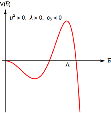
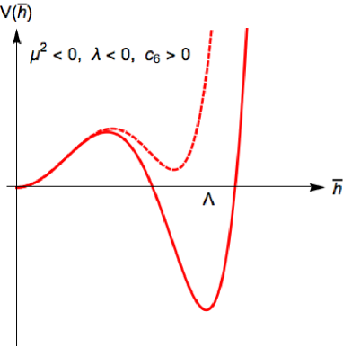
Figure 1: The two kind of instabilities triggered by a sizable $c_{6}$. Left: A negative $c_{6}$ is responsible for a large-field-value instability close to the scale $\Lambda$. Right: The EW minimum is generated by the physics at the cutoff scale $\Lambda$. For large enough $c_{6}>0$, the absolute minimum is in $\bar{h}=0$ (dashed line), and the EW vacuum gets destabilized.

This might suggest that there is a lower and upper bound on $c_{6}$ by the requirement that the EW minimum is the absolute one. However, we are going to argue that there is no such a model-independent bound within a generic EFT. Let us discuss in turn the two kind of instabilities.

2.2.1 Large-field-value instability: $\bar{h}\lesssim\Lambda$

The main observation here is that the very expansion of the scalar potential in powers of $\bar{h}/\Lambda$ in the vicinity of an instability leads to the breakdown of the EFT expansion [40]. This has to be traced back to the fact that when the scalar potential is close to vanish, field configurations $\bar{h}\sim\Lambda$ do not cost prohibitive energy to excite, contrary to the standard case $V(\bar{h}\sim\Lambda)\sim\Lambda^{4}$.

The spurious nature of the $\left|H\right|^{6}$ instability is clearly exemplified by taking the EFT limit of a simple toy model that features, by construction, absolute stability in the full theory [40]. Let $h$ and $\phi$ be two real scalar fields, whose potential reads

$$V(h,\phi)=-\frac{1}{2}m^{2}h^{2}+\frac{1}{4}\lambda h^{4}+\frac{1}{2}M^{2}\phi^{2}+\xi h^{3}\phi+\kappa h^{2}\phi^{2}+\frac{1}{4}\lambda^{\prime}\phi^{4}\,.$$ (17)

Let us consider now the limit $M^{2}\gg m^{2}>0$. The stationary equations can be solved perturbatively for $m^{2}/M^{2}\ll 1$, thus yielding

$$\left\langle h\right\rangle \simeq\left(\frac{m^{2}}{\lambda}\right)^{\frac{1}{2}}\,,$$ (18)

$$\left\langle\phi\right\rangle \simeq-\frac{\xi}{M^{2}}\left(\frac{m^{2}}{\lambda}\right)^{\frac{3}{2}}\ll\left\langle h\right\rangle\,,$$ (19)

which is a global minimum as long as $M^{2}>\frac{9\xi^{2}}{2\lambda^{2}}m^{2}$. Moreover, a sufficient condition for the potential to be bounded from below is

$$\kappa>0\,,\quad\land\quad\lambda>\frac{\xi^{2}}{\kappa}\,,\quad\land\quad\lambda^{\prime}>0\,,$$ (20)

so by choosing the potential parameters as in Eq. (20) it is always possible to ensure that the vacuum in Eqs. (18)–(19) is absolutely stable.

Now we integrate $\Phi$ out. A standard calculation yields

$$V_{\text{EFT}}(h)\simeq-\frac{1}{2}m^{2}h^{2}+\frac{1}{4}\lambda h^{4}-\frac{1}{2}\xi^{2}\frac{h^{6}}{M^{2}+2\kappa h^{2}}\,.$$ (21)

As a consequence of Eq. (20) the EFT potential in Eq. (21) is clearly stable as well. On the other hand, by expanding the denominator of the $h^{6}$ term for $M^{2}\gg 2\kappa h^{2}$, we get

$$V_{\text{EFT}}(h)\simeq-\frac{1}{2}m^{2}h^{2}+\frac{1}{4}\lambda h^{4}-\frac{1}{2}\frac{\xi^{2}}{M^{2}}h^{6}+\frac{\xi^{2}\kappa}{M^{4}}h^{8}+\ldots\,.$$ (22)

Apparently, the $h^{6}$ operator features an instability, which however is not supported by the full renormalizable model in view of the stability conditions in Eq. (20). The key point is that the spurious instability sourced by the $h^{6}$ term does not capture the $\kappa$ dependence, as the appropriate resummation of the geometric series shows in Eq. (21). We hence conclude that it is not possible to set a model-independent bound on $c_{6}$ from the requirement of stability at large field values.

We finally note that a possible gauge-invariant way to realize the toy model in Eq. (17) is given by an Higgs doublet $H\sim(1,2,1/2)$ (where the quantum numbers in the bracket denote the transformation properties under $SU(3)_{c}\times SU(2)_{L}\times U(1)_{Y}$) coupled to an EW quadruplet $\Phi\sim(1,4,-3/2)$ via the scalar potential

$$V(H,\Phi) =-\mu^{2}_{H}\left|H\right|^{2}+\mu^{2}_{\Phi}\left|\Phi\right|^{2}+\lambda_{H}\left|H\right|^{4}+\lambda_{1}\left|H\right|^{2}\left|\Phi\right|^{2}+\lambda_{2}H^{*}H\Phi^{*}\Phi$$

$$+\left(\lambda_{3}HHH\Phi+\text{h.c.}\right)+\lambda_{\Phi}\left|\Phi\right|^{4}+\tilde{\lambda}_{\Phi}\Phi^{*}\Phi\Phi^{*}\Phi\,,$$ (23)

where non-trivial $SU(2)_{L}$ contractions are left understood. We have checked that the same qualitative conclusions obtained within the toy model apply to the more realistic case of Eq. (2.2.1).

2.2.2 Low-scale instability: $\bar{h}=0$

In order to study this case it is more convenient to trade the parameters $\mu^{2}$ and $\lambda$ in terms of the EW vev $v$ and the physical Higgs mass $m_{h}$. Imposing the existence of the EW minimum $\bar{h}=v$ from Eq. (4) and expanding over the Higgs field fluctuations $v\to v+h$, one gets

$$\mu^{2} =\lambda v^{2}+\frac{3}{4}c_{6}v^{2}=\frac{m^{2}_{h}}{2}-\frac{3}{4}c_{6}v^{2}\,,$$ (24)

$$\lambda =\frac{m_{h}^{2}}{2v^{2}}-\frac{3}{2}c_{6}\,.$$ (25)

By substituting $v=246$ GeV and $m_{h}=125$ GeV in Eqs. (24)–(25), we find $\mu^{2}<0$ and $\lambda<0$ as long as $c_{6}\gtrsim 0.17$. This is precisely the situation described in case 3 of Sect. 2.1. By taking an even larger $c_{6}$ the minimum in $\bar{h}=0$ might become the absolute one (cf. Fig. 1). This happens for (see also [34])

$$V^{(6)}(v)=\frac{c_{6}v^{4}-m^{2}_{h}v^{2}}{8}>0=V^{(6)}(\bar{h}=0)\,,$$ (26)

corresponding to $c_{6}\gtrsim 0.26$. However, for a weakly coupled theory where $c_{6}$ scales like $v^{2}/\Lambda^{2}$, such value of $c_{6}$ implies a very low cutoff scale of $\Lambda\lesssim 480$ GeV, thus making the application of the EFT questionable. On the other hand, even admitting for a strongly-coupled origin of $c_{6}$, higher-order operators cannot be consistently neglected for assessing the global structure of the Higgs potential away from the EW minimum, since $\left|H\right|^{6}$ gives access only up to the sixth derivative of the potential on the EW minimum.

2.3 Perturbativity bounds

On general grounds, one expects that too large values of the Higgs self-couplings are bounded by perturbativity arguments. In the following, we compare two criteria: the former is based on the partial-wave unitarity of the Higgs bosons’ scattering amplitude, while the latter consists in the requirement that the loop corrections to the Higgs self-interaction vertices are smaller than the tree-level ones. Both criteria yield a similar result.

2.3.1 Partial-wave unitarity

The $2\to 2$ Higgs bosons’ scattering amplitude grows for large values of the Higgs self-couplings, eventually leading to unitarity violation and hence to the breakdown of the perturbative expansion. Using the modified Lagrangian in Eq. (1), the $hh\to hh$ scattering amplitude reads (see also Fig. 2)

$$\mathcal{M}=-\lambda_{hhh}^{2}\left(\frac{1}{s-m_{h}^{2}}+\frac{1}{t-m_{h}^{2}}+\frac{1}{u-m_{h}^{2}}\right)-\lambda_{hhhh}\,,$$ (27)

with $s$, $t$, $u$ denoting the standard Mandelstam variables defined in the center of mass frame. In particular, we also have $t=-(s-4m_{h}^{2})\sin^{2}\frac{\theta}{2}$ and $u=-(s-4m_{h}^{2})\cos^{2}\frac{\theta}{2}$, where $\sqrt{s}$ is the center of mass energy and $\theta$ is the azimuthal angle with respect to the colliding axis.

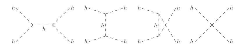
Figure 2: $hh\to hh$ scattering amplitudes: $s+t+u$ channels $+$ 4-vertex (4vrtx) contributions.

The $J=0$ partial wave is found to be

$$a^{0}_{hh\to hh}=-\frac{1}{2}\frac{\sqrt{s(s-4m^{2}_{h})}}{16\pi s}\left[\lambda_{hhh}^{2}\left(\frac{1}{s-m_{h}^{2}}-2\frac{\log\frac{s-3m^{2}_{h}}{m^{2}_{h}}}{s-4m^{2}_{h}}\right)+\lambda_{hhhh}\right]\,,$$ (28)

where we paid attention to keep the kinematical factors which makes the amplitude to vanish at threshold ($\sqrt{s}=2m_{h}$) and we multiplied by an extra $1/2$ factor due to the presence of identical particles in the initial and final state (see e.g. [48] for a collection of relevant formulae). Following standard arguments [49, 50], perturbative unitarity bounds are obtained by requiring $\left|\mbox{Re}\,{a^{0}_{hh\to hh}}\right|<1/2$.

The bound is displayed in Fig. 3 for the orthogonal cases in which either $\lambda_{hhh}$ (upper plots) or $\lambda_{hhhh}$ (lower plots) is modified with respect to the SM case. Note that the situation is qualitatively different for the two cases: being $h^{3}$ a relevant operator, the unitarity bound on $\lambda_{hhh}$ is maximized at low energy, while in the case of $h^{4}$ the partial wave grows with energy reaching an asymptotic value at $\sqrt{s}\to\infty$. In particular, from the right-side plots in Fig. 3 we read the following unitarity bounds

$$\left|\lambda_{hhh}/\lambda^{\rm SM}_{hhh}\right|\lesssim 6.5\qquad\text{and}\qquad\left|\lambda_{hhhh}/\lambda^{\rm SM}_{hhhh}\right|\lesssim 65\,.$$ (29)

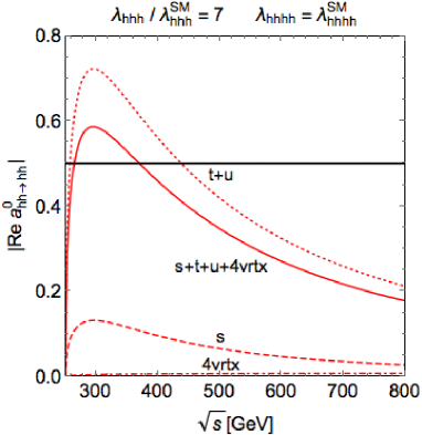
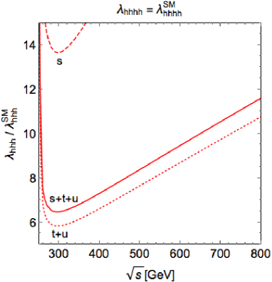
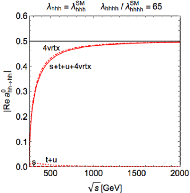
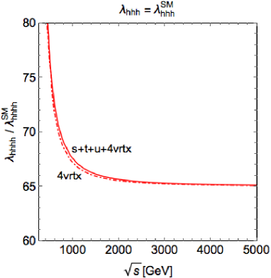
Figure 3: Up/Left: Kinematical dependence of $\left|\mbox{Re}\,{a^{0}_{hh\to hh}}\right|$ for the reference values $\lambda_{hhh}/\lambda_{hhh}^{\rm SM}=7$ and $\lambda_{hhhh}=\lambda_{hhhh}^{\rm SM}$. Up/Right: Partial-wave unitarity bound $\left|\mbox{Re}\,{a^{0}_{hh\to hh}}\right|<1/2$ on $\lambda_{hhh}/\lambda_{hhh}^{\rm SM}$ as a function of $\sqrt{s}$ and for $\lambda_{hhhh}=\lambda_{hhhh}^{\rm SM}$. Down/Left: Kinematical dependence of $\left|\mbox{Re}\,{a^{0}_{hh\to hh}}\right|$ for the reference values $\lambda_{hhhh}/\lambda_{hhhh}^{\rm SM}=65$ and $\lambda_{hhh}=\lambda_{hhh}^{\rm SM}$. Down/Right: Partial-wave unitarity bound $\left|\mbox{Re}\,{a^{0}_{hh\to hh}}\right|<1/2$ on $\lambda_{hhhh}/\lambda_{hhhh}^{\rm SM}$ as a function of $\sqrt{s}$ and for $\lambda_{hhh}=\lambda_{hhh}^{\rm SM}$. Dashed, dotted, dot-dashed and full curves denote respectively the $s$, $t+u$, $4$vrtx and $s+t+u+4$vrtx contribution to the partial wave. Note that $s$ and $4$vrtx have the opposite sign of $t+u$ (cf. Eq. (28)).

Of course, one expects that new physics effects should modify at the same time both $\lambda_{hhh}$ and $\lambda_{hhhh}$. However, since the $h^{3}$ and $h^{4}$ operators dominate the partial wave in two well-separated energy regimes they cannot cancel each other over the whole range of $\sqrt{s}$. Hence, since we require perturbativity at any value of $\sqrt{s}$, the bounds in Eq. (29) hold also in more general situations (as we have checked numerically by employing the full expression in Eq. (28)).

Let us inspect, for instance, the case where the modified SM potential arises from the operator $\left|H\right|^{6}$ as in Eq. (3). In such a case we have

$$\lambda_{hhh} =\lambda^{\rm SM}_{hhh}+6\,c_{6}v\simeq\lambda^{\rm SM}_{hhh}\left(1+7.8\,c_{6}\right)\,,$$ (30)

$$\lambda_{hhhh} =\lambda^{\rm SM}_{hhhh}+36\,c_{6}\simeq\lambda^{\rm SM}_{hhhh}\left(1+47\,c_{6}\right)\,.$$ (31)

The perturbativity bound coming from the $h^{3}$ ($h^{4}$) vertex in Eq. (29) translates into $\left|c_{6}\right|\lesssim 0.71\ (1.4)$.

2.3.2 Loop-corrected vertices

An alternative way to assess perturbativity is by requiring that the loop-corrected trilinear scalar vertex is smaller (in absolute value) than $\lambda_{hhh}$. If that were not the case, we clearly could not reliably use perturbation theory whenever $\lambda_{hhh}$ entered some physical process. A similar criterium was employed for trilinear scalar interactions in Ref. [48], by setting to zero the external momenta of the 3-point function. Following the same argument, we obtain

$$\Delta\lambda_{hhh}(p_{i}\to 0)=\frac{1}{32\pi^{2}}\lambda_{hhh}^{3}\frac{1}{m_{h}^{2}}.$$ (32)

By requiring that $|\Delta\lambda_{hhh}/\lambda_{hhh}|<1$, the trilinear Higgs self-coupling is bounded by

$$\left|\lambda_{hhh}/\lambda_{hhh}^{\text{SM}}\right|\lesssim 12\,.$$ (33)

A stronger perturbativity bound can be obtained by looking at the full kinematical dependence of the trilinear vertex at the one-loop order. Considering the finite one-loop contribution due to $\lambda_{hhh}$ we obtain

$$\Delta\lambda_{hhh}(\sqrt{s},m_{h})=-\frac{1}{16\pi^{2}}\lambda_{hhh}^{3}C_{0}(m_{h}^{2},m_{h}^{2},s;m_{h},m_{h},m_{h})\,,$$ (34)

where $C_{0}$ is a scalar Passarino-Veltman function (defined according to the conventions of Ref. [51]) and $\sqrt{s}$ denotes the off-shell momentum of a Higgs boson line. Since we only took into account the loop correction where the $\lambda_{hhh}$ coupling occurs, there are no divergent contributions, and we neglected scheme-dependent finite terms. It should be understood that what we aim at is not a proper calculation of the quantum corrections to $\lambda_{hhh}$, but rather a simple estimate of the validity of perturbation theory. The reason why an estimate based solely on the contribution in Eq. (34) is reasonable is the following: $i)$ in the large $\lambda_{hhh}$ limit, where the perturbativity bound is relevant, pure SM contributions are subleading and $ii)$ even though by gauge invariance one should worry about simultaneous $\lambda_{hhhh}$ corrections, these are divergent and hence scheme dependent. Then, the estimate in Eq. (34) would be inaccurate only if the finite contribution (in a given renormalization scheme) due to $\lambda_{hhhh}$ were to cancel the one stemming from $\lambda_{hhh}$ to a large extent and over the full kinematical range. This however is very unlikely, given that the corrections have a very different kinematical dependence.

The perturbativity bound, denoted by $\lambda^{*}_{hhh}$, is shown in Fig. 4 as a function of $\sqrt{s}$. Note that above threshold, $\sqrt{s}>2m_{h}$, $C_{0}$ develops an imaginary part and hence we have separately considered both the real and imaginary contribution to the bound. Since one should require that perturbativity must hold for any value of $\sqrt{s}$, the bound is maximized close to threshold and reads

$$\left|\lambda_{hhh}/\lambda_{hhh}^{\text{SM}}\right|\lesssim 6\,,$$ (35)

which is consistent with the (conceptually different) constraint obtained in Eq. (29).

Figure 4: Perturbativity bound $\lambda_{hhh}<\lambda^{*}_{hhh}$ from the loop-corrected trilinear vertex as a function of $\sqrt{s}$. Full and dashed curves denote respectively the real ($\left|\mbox{Re}\,(\Delta\lambda_{hhh})/\lambda_{hhh}\right|<1$) and imaginary ($\left|\mbox{Im}\,(\Delta\lambda_{hhh})/\lambda_{hhh}\right|<1$) contributions to the bound due to the vertex correction in Eq. (34).

A similar argument can be used to set a perturbativity bound on $\lambda_{hhhh}$ by looking at its beta function (see e.g. [52]). By requiring $\left|\beta_{\lambda_{hhhh}}/\lambda_{hhhh}\right|<1$, we get $\left|\lambda_{hhhh}\right|<\frac{16\pi^{2}}{3}\simeq 53$. Normalizing the latter with respect to the SM value implies

$$\left|\lambda_{hhhh}/\lambda^{\rm SM}_{hhhh}\right|\lesssim 68\,,$$ (36)

which again is consistent with Eq. (29).

In the end, given the impossibility of setting genuine model-independent bounds on $\lambda_{hhh}$ beyond perturbativity, we focus in the next section on UV complete scenarios when investigating the question of the maximal value of the triple Higgs coupling. We focus for simplicity on weakly coupled models, as they retain a higher degree of predictivity and we have full control of the theory.

3 UV complete models

If the new degrees of freedom are very light, they can affect the Higgs-pair production process in different ways (like e.g. resonant production [53, 54, 55, 56, 57, 58, 59, 60] or by scalar/fermionic contributions to the gluon fusion loop [61, 62, 63]) and the dominant effect does not need to be associated with the $\lambda_{hhh}$ coupling deviation. Hence, we focus on the case where the new physics is above the EW scale, but not necessarily yet in the EFT regime where the effects are expected to decouple rapidly. The latter language is nonetheless useful in order to classify the representations which are potentially more prone to induce a large effect: at tree level there are basically three class of diagrams (cf. Fig. 5) which can generate $\left|H\right|^{6}$ by integrating out a heavy new scalar degree of freedom.

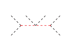
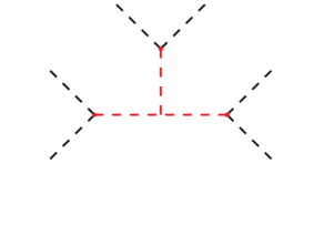
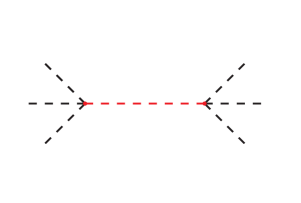
Figure 5: Tree-level generation of the $\left|H\right|^{6}$ operator (external lines, black) obtained by integrating out new scalar degrees of freedom (internal propagators, red).

Here, we concentrate on trilinear Higgs self-coupling modifications generated by $\left|H\right|^{6}$, since they uniquely modify the Higgs self-couplings. Also the operator $\partial_{\mu}(H^{\dagger}H)\partial^{\mu}(H^{\dagger}H)$ gives a contribution to the shift in the trilinear Higgs self-coupling, but it modifies all other Higgs couplings as well.

In fact, the connecting motive between the diagrams in Fig. 5 turns out to be a tadpole operator of the type $\mathcal{O}_{\Phi}=\Phi f(H)$, where $f(H)$ is a string of Higgs fields (or their charged conjugates). The full list of scalar extensions that couple linearly to $H$ can be found in Table 1 (see also Refs. [66, 67, 68]), where hyper-chargeless multiplets are understood to be real. For simplicity, we will focus on one-particle extensions of the SM in order to point out their features in a clear way.

$\Phi$	$\mathcal{O}_{\Phi}$
$(1,1,0)$	$\Phi HH^{\dagger}$
$(1,2,\tfrac{1}{2})$	$\Phi HH^{\dagger}H^{\dagger}$
$(1,3,0)$	$\Phi HH^{\dagger}$
$(1,3,1)$	$\Phi H^{\dagger}H^{\dagger}$
$(1,4,\tfrac{1}{2})$	$\Phi HH^{\dagger}H^{\dagger}$
$(1,4,\tfrac{3}{2})$	$\Phi H^{\dagger}H^{\dagger}H^{\dagger}$

Table 1: List of new scalars $\Phi$ inducing a tree-level modification of the triple-Higgs coupling via the tadpole operator $\mathcal{O}_{\Phi}$.

Another useful way to understand the origin of the trilinear Higgs self-coupling modification, which does not rely on the EFT language is the following: the tadpole operator will unavoidably generate a vev for $\Phi$, and the neutral components $h^{0}\subset H$ and $\phi^{0}\subset\Phi$ will mix via the tadpole operator itself. After projecting the two neutral components on the Higgs boson mass eigenstate, namely $h^{0}\to h\cos\theta$ and $\phi^{0}\to h\sin\theta$, we have the following contribution to the triple-Higgs vertex

$$\Delta\lambda_{hhh}=\mu_{\Phi}\sin\theta\cos^{2}\theta\qquad\text{or}\qquad\lambda_{\Phi}v\sin\theta\cos^{3}\theta\,,$$ (37)

depending whether the tadpole operator is $d=3$ ($\mu_{\Phi}$ coupling) or $d=4$ ($\lambda_{\Phi}$ coupling). Since there is a single suppression from the mixing angle, bounded at the level of $\theta\lesssim 0.3$ from Higgs coupling measurements, the tadpole interaction is expected to yield the largest contribution, while other mixing operators in the scalar potential entail extra suppressions from $\sin\theta$. We can also naively estimate the contribution in the following way: assuming that $\mu_{\Phi}/v\lesssim 4\pi$ and $\lambda_{\Phi}\lesssim 4\pi$ by perturbativity we get

$$\frac{\Delta\lambda_{hhh}}{\lambda^{\text{SM}}_{hhh}}\lesssim 4\pi\sin\theta\cos^{2}\theta\frac{v^{2}}{3m_{h}^{2}}\sim 4\,.$$ (38)

To make this estimate more precise, we will look in detail at two paradigmatic examples among those in Table 1: one model which exhibits a tree-level custodial symmetry (singlet case, Sect. 3.1) and one which does not (triplet case, Sect. 3.2).

A notable feature of tadpole interactions is that, being “odd” in $\Phi$, they are potentially bounded by vacuum stability considerations. Remarkably, we find that vacuum stability is never a crucial discriminant for bounding the largest value of $\lambda_{hhh}$, because whenever the tadpole coupling is large the instability can be tamed by large (within the perturbativity domain) quartic couplings. For this reason we find it relevant to discuss in Sect. 3.3 a class of loop-induced trilinear Higgs self-couplings that arise due to vector-like fermions, where one can establish a direct connection between $\lambda_{hhh}$ and the vacuum instability.

3.1 Tree-level custodially symmetric cases

Among the cases in Table 1, the singlet and the doublet do not violate custodial symmetry at tree level and hence have the chance to yield the largest contribution to $\lambda_{hhh}$. We will discuss in detail the singlet case, while we only comment on the case of the doublet towards the end of the subsection. The scalar potential reads

$$V(H,\Phi)=\mu_{1}^{2}|H|^{2}+\lambda_{1}|H|^{4}+\frac{1}{2}\mu_{2}^{2}\Phi^{2}+\mu_{4}|H|^{2}\Phi+\frac{1}{2}\lambda_{3}|H|^{2}\Phi^{2}+\frac{1}{3}\mu_{3}\Phi^{3}+\frac{1}{4}\lambda_{2}\Phi^{4}\,,$$ (39)

where we have omitted a tadpole term for the singlet field, as it can be reabsorbed in the singlet vev by a field redefinition.

In fact, the $\mu_{4}$ coupling unavoidably induces a vev for $\Phi$ and also leads to a mixing between $H$ and $\Phi$. In Appendix A.1 we give the tadpole equations and we define the mixing angle $\theta$ between the singlet and doublet fields. Some of the parameters of the potential can be expressed in terms of the physical masses and vevs and their mixing angle. We chose as input parameters

$$v_{\scriptscriptstyle H}=246.2\text{ GeV}\,,\;\;\;v_{\scriptscriptstyle S}\,,\;\;\;m_{1}=125\text{ GeV}\,,\;\;\;m_{2}\,,\;\;\;\theta\,,\;\;\;\lambda_{2}\,,\;\;\;\lambda_{3}\,.$$ (40)

Their relations to the other parameters of the potential can be found in Appendix A.1. Note that the scenario in which the SM-like Higgs boson is heavier than the singlet-like scalar is phenomenologically viable as well, but we will restrict ourselves to the case $m_{1}\ll m_{2}$. The reason being that we want to discuss deviations to the Higgs pair production process that are mainly stemming from the trilinear Higgs self-coupling, while the contribution from the exchange of the singlet-like Higgs boson in the triangle diagrams is suppressed. For discussion on resonant Higgs pair production in the singlet model we refer to Refs. [53, 54, 55, 56, 57, 58, 59, 60].

The trilinear Higgs self-coupling is given by

$$\lambda_{hhh} = 6\lambda_{1}v_{\scriptscriptstyle H}\cos^{3}\theta-(3\mu_{4}+3\lambda_{3}v_{\scriptscriptstyle S})\cos^{2}\theta\sin\theta+3\lambda_{3}v_{\scriptscriptstyle H}\cos\theta\sin^{2}\theta-\sin^{3}\theta(2\mu_{3}+6v_{\scriptscriptstyle S}\lambda_{2})$$ (41)

$$= \lambda_{hhh}^{\rm SM}\cos\theta\left[1+\sin^{2}\theta\left(\frac{\lambda_{3}v_{\scriptscriptstyle H}^{2}}{m_{1}^{2}}-1\right)+\sin^{4}\theta\frac{v_{\scriptscriptstyle H}^{2}}{3v_{\scriptscriptstyle S}^{2}}\left(1-\frac{m_{2}^{2}}{m_{1}^{2}}\right)\right.$$

$$- \left.\frac{v_{\scriptscriptstyle H}}{3v_{\scriptscriptstyle S}}\frac{\sin^{3}\theta}{\cos\theta}\left(2\sin^{2}\theta+2\cos^{2}\theta\frac{m_{2}^{2}}{m_{1}^{2}}-\frac{\lambda_{3}v_{\scriptscriptstyle H}^{2}}{m_{1}^{2}}+\frac{2v_{\scriptscriptstyle S}^{2}\lambda_{2}}{m_{1}^{2}}\right)\right]\,,$$

where in the last step we expressed $\lambda_{hhh}$ in terms of the input parameters in Eq. (40).

In order to make contact with the discussion at the beginning of Sect. 3 on the importance of tadpole operators for enhancing the trilinear Higgs self-coupling, let us compare the expression in Eq. (41) with the one obtained in the $\mathbb{Z}_{2}$-symmetric limit with $\mu_{3,4}\to 0$, which yields

$$\lambda_{hhh}^{\mathbb{Z}_{2}\text{--symmetric}}=\lambda_{hhh}^{\rm SM}\left(\cos^{3}\theta-\sin^{3}\theta\frac{v_{\scriptscriptstyle H}}{v_{\scriptscriptstyle S}}\right)\,.$$ (42)

It is thus evident that the shift in the trilinear Higgs self-coupling can be much larger for the general singlet potential with tadpole terms. In the last step of Eq. (41) we see indeed that potentially large contributions can arise from sizable values of $\lambda_{3}$.

In the following we will discuss which values the trilinear Higgs self-coupling can take, by accounting for several constraints.

3.1.1 Indirect bounds

The model parameters can be restricted by EW precision tests, Higgs coupling measurements, perturbativity arguments and vacuum stability. These will then indirectly constrain the trilinear Higgs self-coupling in the model.

EW precision tests:
In Ref. [71] it was pointed out that the measurement of the $W$ boson mass constrains the scalar singlet model more strongly than a fit on the $S$, $T$, $U$ parameters. Even though the study in Ref. [71] concerns a $\mathbb{Z}_{2}$ symmetric potential, we can use the bounds here, since at the one-loop order the additional parameters in the scalar potential do not play any role for the gauge boson vacuum polarizations. For $m_{2}>800\text{ GeV}$, Ref. [71] finds the bound $|\sin\theta|<0.2$.

Higgs coupling measurements:
The Higgs production and decay rates are modified with respect to the SM by a universal factor

$$\sigma(pp\to h+X) =\cos^{2}\theta\,\sigma_{\rm SM}(pp\to h+X)\,,$$ (43)

$$\Gamma(h\to XX) =\cos^{2}\theta\,\Gamma_{\rm SM}(h\to XX)\,.$$ (44)

If the SM-like Higgs boson corresponds to the lightest eigenstate, its branching ratios are not modified compared to the SM. In Ref. [72] a limit on $\sin^{2}\theta<0.12$ at 90% C.L. from Higgs signal measurements is given. This limit turns out to be stronger than the limits from direct searches of the heavier Higgs boson, as long as $m_{2}>450\ \text{GeV}$ [73], such that we will not need to take the latter into account for the parameter space we consider.

Perturbativity:
For large enough potential couplings unitarity is violated in tree-level scattering processes, thus signalling the breakdown of perturbation theory. Simple criteria can be derived from the $ii\to jj$ scattering, with $i$ and $j$ running over the (real) Higgs and singlet fields. By requiring $\left|\text{Re}\,a_{0}\right|<1/2$ for the eigenvalues of the $J=0$ partial-wave scattering matrix, we derive the following constraint in the high-energy limit

$$3\left(\lambda_{1}+\lambda_{2}\right)\pm\sqrt{9\left(\lambda_{1}-\lambda_{2}\right)^{2}+\lambda_{3}^{2}}<16\pi\,.$$ (45)

The dimensionful parameters $\mu_{3}$ and $\mu_{4}$ can be restricted by unitarity arguments as well. However, being associated to super-renormalizable operators the bounds are maximized at low energies, where the possible presence of resonances actually requires a careful treatment of the pole singularities. Following the argument of Ref. [48], in order to define the perturbative domain of $\mu_{3}$ and $\mu_{4}$ we require instead that the one-loop corrected trilinear scalar couplings at zero external momenta remain smaller than the tree-level ones. In the $SU(2)$ limit we obtain

$$\frac{\left|\mu_{4}\right|}{\text{max}\,\left(\left|\mu_{1}\right|,\left|\mu_{2}\right|\right)}<4\pi\,,\quad\land\quad\left|\frac{\mu_{3}}{\mu_{2}}\right|<4\pi\,.$$ (46)

The saturation of the bounds in Eqs. (45)–(46) correspond to an extreme situation, where we progressively enter a strongly-coupled regime for which the perturbative calculation does not make sense anymore. For this reason, we will also present the results in another regime where we keep the couplings significantly smaller. For that we use in Eq. (46) the replacement $4\pi\to 1$ and in the scan we restrict $0<\lambda_{2}<1/6$ and $|\lambda_{3}|<1$.

Vacuum stability:
The requirement that the scalar potential is bounded from below imposes the following conditions on the quartic scalar interactions

$$\lambda_{1}>0\,,\quad\land\quad\lambda_{2}>0\,,\quad\land\quad\lambda_{3}>-2\sqrt{\lambda_{2}\lambda_{1}}\,.$$ (47)

The study of the minima of the scalar potential exhibits a rich structure, with new local minima (e.g. in $h=0$) that arise in some regions of the parameter space and which might eventually destabilize the EW vacuum. A detailed analysis of the vacuum structure at tree level can be found in Refs. [74, 55]. We check for vacuum stability by using Vevacious [75, 76], with a model file generated with SARAH [77, 78, 79, 80, 81].

3.1.2 Results

In order to show the results we perform a scan over the parameter space. The universally scanned parameters in both the cases are

$$m_{1}=125\text{ GeV},\hskip 14.22636pt\;800\text{ GeV}<m_{2}<2000\text{ GeV},\;$$ (48)

$$v_{\scriptscriptstyle H}=246.2\text{ GeV},\hskip 14.22636pt\;|v_{\scriptscriptstyle S}|<m_{2},\hskip 14.22636pt\;0.9<\cos\theta<1\,.$$

We will perform two different scans. In the first one we use the maximally allowed values according to the perturbativity argument

$$\begin{split}\text{Scan 1: }\hskip 14.22636pt0<\lambda_{2}<\frac{8}{3}\pi,\hskip 14.22636pt\;|\lambda_{3}|<16\pi,\end{split}$$ (49)

and reject all points that do not fulfil Eq. (45), Eq. (46) and Eq. (47). In the second scan we restrict ourselves to a weakly-coupled scenario and scan the input parameters

$$\begin{split}\text{Scan 2: }\hskip 14.22636pt0<\lambda_{2}<1/6,\hskip 14.22636pt\;|\lambda_{3}|<1,\end{split}$$ (50)

together with $|\mu_{4}|/\text{max}(|\mu_{1}|,|\mu_{2}|)<1$ and $|\mu_{3}/\mu_{2}|<1$.

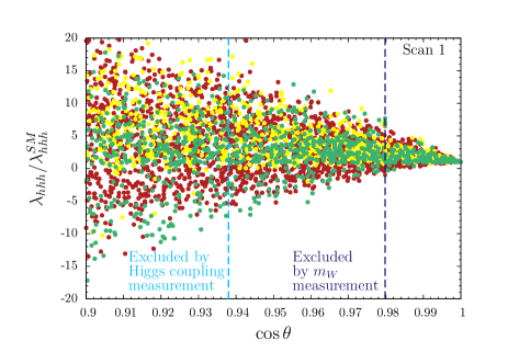
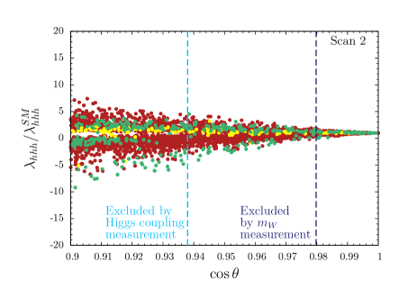
Figure 6: Left: The trilinear Higgs self coupling normalised to the SM reference value for scan 1 (strongly-coupled regime). The red/yellow/green points correspond respectively to unstable/metastable/stable configurations. The dashed vertical lines indicate the bounds on $\cos\theta$ from the respective experimental measurements. Right: Same as in left panel, but for scan 2 (weakly-coupled regime).

In Fig. 6 the trilinear Higgs self coupling normalised to the SM coupling is shown. The color code of the points indicate whether they correspond to a stable, metastable or unstable vacuum configuration. By accounting for the bounds of the $m_{W}$ boson measurement we find the following range for the allowed trilinear Higgs self-coupling:

Scan 1: $$-1.5<\lambda_{hhh}/\lambda_{hhh}^{\rm SM}<8.7\,,$$ (51)

Scan 2: $$\,-0.3<\lambda_{hhh}/\lambda_{hhh}^{\rm SM}<2.0\,.$$ (52)

In fact, the largest value of the trilinear Higgs self-coupling is crucially related to the perturbativity domain. The bounds on the trilinear Higgs self-coupling obtained from scan 1 should hence be treated with care, as they are very close to the non-perturbative regime and loop corrections can be expected to be large. This can be easily understood looking at the formulae in Eq. (41). By allowing for rather large values of e.g. $\lambda_{3}$ we can get much larger deviations. Note that we find here a larger value for $\lambda_{hhh}/\lambda_{hhh}^{\rm SM}$ as in Sect. 2.3, since we require a weaker perturbativity criterium in Eq. (46), corresponding to the one in Eq. (33). Indeed, due to the possible presence of resonances which requires a careful treatment of the pole singularities we could not apply the bound in Eq. (29) from partial-wave unitarity in a straightforward manner. On the other hand, as it can be inferred from Fig. 6, the requirement of a stable vacuum has only a very small impact on the bound of the trilinear Higgs self-coupling. The little impact of vacuum stability can be understood by the fact that the presence of many parameters in the scalar potential basically uncorrelates the stability conditions from the value of the trilinear Higgs self-coupling.

At this point, we would like to comment on previous studies in the context of the scalar singlet. In Ref. [82], deviations for $\lambda_{hhh}/\lambda_{hhh}^{\rm SM}$ up to $-10$ were found. Note however that much weaker limits on the mixing angle $\theta$ were employed, since the bound stemming from the $m_{W}$ measurement was not used. In addition, weaker bounds from the Higgs coupling measurements were employed. In Ref. [83, 84] one-loop corrections to the trilinear Higgs self-coupling were computed. They can give large corrections (even up to 100%) from non-decoupling effects in the Higgs boson loops if $\lambda_{3}v_{\scriptscriptstyle H}^{2}\gg\mu_{2}^{2}$ [85]. This is not surprising, given the fact that one is saturating the perturbativity limit where loop effects are not under control.

We conclude with a few remarks on the other custodial symmetric case, namely the two-Higgs doublet model (2HDM). The question of the trilinear Higgs self-coupling was addressed in detail in the context of the $\mathbb{Z}_{2}$ symmetric case [86, 87], where it was shown that the expected deviations are well below those allowed in the general singlet model. On the other hand, a full study in the context of the general 2HDM (including the $\Phi HH^{\dagger}H^{\dagger}$ tadpole operator) is still missing to our knowledge (see however [88] for a qualitative study). In such a case we expect potentially large deviations. We leave this study for future investigations.

3.2 Tree-level custodially violating cases

We shall discuss the cases corresponding to the last four rows in Table 1 altogether, since they have in common the fact that the tadpole term $\Phi f(H)$ contributing to a potentially sizable triple Higgs self-coupling generates a custodial-breaking vev for $\Phi$, which is strongly bounded by EW precision tests.

Let us exemplify the analysis for the case of a real EW triplet with zero hypercharge, $\Phi\sim(1,3,0)$. The scalar potential reads (see e.g. [89])

$$V(H,\Phi)=\mu_{1}^{2}\left|H\right|^{2}+\frac{1}{2}\mu_{2}^{2}\left|\Phi\right|^{2}+\lambda_{1}\left|H\right|^{4}+\frac{1}{4}\lambda_{2}\left|\Phi\right|^{4}+\frac{1}{2}\lambda_{3}\left|H\right|^{2}\left|\Phi\right|^{2}+\mu_{4}H^{\dagger}\sigma^{\alpha}H\Phi^{\alpha}\,,$$ (53)

where, without loss of generality, we can take $\mu_{4}>0$ by reabsorbing the sign in the definition of $\Phi$. The minimization of the potential and the calculation of the scalar spectrum is deferred to Appendix A.2. In particular, we can choose the following independent observables as parameter inputs for the model

$$v_{\scriptscriptstyle H}=\sqrt{v^{2}-4v_{\scriptscriptstyle T}^{2}}\,,\;\;\;v_{\scriptscriptstyle T}<3.5\ \text{GeV}\,,\;\;\;m_{1}=125\text{ GeV}\,,\;\;\;m_{2}\,,\;\;\;m_{h^{\pm}}\,,\;\;\;\theta\,,$$ (54)

where $v=246.2$ GeV. The trilinear Higgs self-coupling is given by

$$\lambda_{hhh} = 6\lambda_{1}v_{\scriptscriptstyle H}\cos^{3}\theta+3\left(\mu_{4}-\lambda_{3}v_{\scriptscriptstyle T}\right)\cos^{2}\theta\sin\theta+3\lambda_{3}v_{\scriptscriptstyle H}\cos\theta\sin^{2}\theta-6\lambda_{2}v_{\scriptscriptstyle T}\sin^{3}\theta$$

$$= \frac{3m_{1}^{2}}{v_{\scriptscriptstyle H}}\cos\theta\left[1+\left(\frac{2m_{h^{\pm}}^{2}v_{\scriptscriptstyle H}^{2}}{(v_{\scriptscriptstyle H}^{2}+4v_{\scriptscriptstyle T}^{2})m_{1}^{2}}-1\right)\sin^{2}\theta+\left(\frac{m_{h^{\pm}}^{2}v_{\scriptscriptstyle H}^{2}}{(v_{\scriptscriptstyle H}^{2}+4v_{\scriptscriptstyle T}^{2})m_{1}^{2}}-1\right)\frac{v_{\scriptscriptstyle H}}{v_{\scriptscriptstyle T}}\frac{\sin^{3}\theta}{\cos\theta}\right]\,,$$

where in the last step we expressed $\lambda_{hhh}$ in terms of the parameters in Eq. (54).

3.2.1 Indirect bounds

As in the singlet case, we are going to consider in turn EW precision tests, Higgs coupling measurements, perturbativity arguments and vacuum stability in order to constrain the trilinear Higgs self-coupling in the triplet model.

EW precision tests:
The main bound comes from the tree-level modification of the $\rho$ parameter. In the SM the custodial symmetry of the Higgs potential ensures the tree-level relation $\rho\equiv m_{W}^{2}/m_{Z}^{2}\cos^{2}\theta_{W}=1$. Extra sources of custodial symmetry breaking which cannot be accounted within the SM are described by the $\rho_{0}\equiv\rho/\rho_{\rm{SM}}$ parameter. Provided that the new physics which yields $\rho_{0}\neq 1$ does not significantly affect the SM radiative corrections, a global fit to EW observables yields $\rho_{0}^{\rm(fit)}=1.00037\pm 0.00023$ [92]. In the triplet model one has

$$\rho^{\rm{tree}}_{0}=1+4\frac{v_{\scriptscriptstyle T}^{2}}{v_{\scriptscriptstyle H}^{2}}\,,$$ (56)

and using the $2\sigma$-level bound from $\rho_{0}^{\rm(fit)}$ we obtain $v_{\scriptscriptstyle T}<3.5$ GeV.

Higgs coupling measurements:
In case of a triplet, the Higgs couplings are modified by $\cos\theta$, while the gauge-Higgs boson couplings get a contribution from the triplet admixture proportional to $\sin\theta$. The mixing angle between the doublet and triplet scalar fields is necessarily rather small since $\theta\to 0$ for $v_{\scriptscriptstyle T}/v_{\scriptscriptstyle H}\to 0$. This means that the tree-level Higgs couplings to fermions and gauge bosons are basically unmodified. The charged Higgs boson contributes to the loop-induced $h\to\gamma\gamma$ and $h\to Z\gamma$ decay. Its contribution is however negligible for $m_{h^{\pm}}\gtrsim 300\text{ GeV}$ [67]. Perturbativity requirements and EW precision tests lead to rather small mass splittings of $\mathcal{O}$(few GeV) between the neutral and charged components of the triplet. Since we are interested in a non-resonant region of phase space for the Higgs pair production process, we consider scenarios with significantly larger charged Higgs boson masses $m_{h^{\pm}}$ and $m_{2}$. Furthermore, we check for exclusion limits of additional Higgs bosons by means of the code HiggsBounds [93, 94, 95]. It turns out however that for our parameter space scan, no points are excluded.

Perturbativity:
The adimensional couplings in the potential of Eq. (53) are bounded by perturbative unitarity. Looking at correlated matrix of $2\to 2$ scattering processes one finds [96]

$$\lambda_{1}<4\pi\,,\qquad\lambda_{2}<4\pi\,,\qquad\lambda_{3}<8\pi\,,\qquad 6\lambda_{1}+5\lambda_{2}\pm\sqrt{(6\lambda_{1}-5\lambda_{2})^{2}+12\lambda_{3}^{2}}<16\pi\,.$$ (57)

For the dimensionful parameter $\mu_{4}$ we estimate the finite loop corrections to the $\mu_{4}$ vertex at zero external momenta and require it to be smaller than the tree-level value. In the $SU(2)_{L}$ limit we obtain

$$\frac{\left|\mu_{4}\right|}{\text{max}\,\left(\left|\mu_{1}\right|,\left|\mu_{2}\right|\right)}<4\pi\,.$$ (58)

Vacuum stability:

By requiring that the potential is bounded from below, we obtain the conditions

$$\lambda_{1}>0,\hskip 14.22636pt\land\hskip 14.22636pt\lambda_{2}>0,\hskip 14.22636pt\land\hskip 14.22636pt\lambda_{3}>-2\sqrt{\lambda_{1}\lambda_{2}}\,.$$ (59)

Also the massive coupling $\mu_{4}$ can destabilize the potential, if too large. We check for vacuum stability using Vevacious [75, 76], with a model file generated with SARAH [77, 78, 79, 80, 81].

In principle, one should check also for charge breaking (CB) minima. For a CB stationary point we find the necessary condition (cf. Appendix A.2 for notation)

$$v^{\eta_{+}}_{\scriptscriptstyle{CB}}\left(\frac{\lambda_{3}}{2}v_{\scriptscriptstyle{H,CB}}^{2}+\mu_{2}^{2}+\lambda_{2}v^{2}_{\scriptscriptstyle{T,CB}}+2\lambda_{2}|v^{\eta_{+}}_{\scriptscriptstyle{CB}}|^{2}\right)=0\,,$$ (60)

where the subscript “CB” refers to the vevs in the CB minimum and $\langle\eta_{+}\eta_{-}\rangle=|v^{\eta_{+}}_{\scriptscriptstyle{CB}}|^{2}$. In addition, from the other stationary equations we find that $v_{\scriptscriptstyle{H,CB}}=0$ for $v^{\eta_{+}}_{\scriptscriptstyle{CB}}\neq 0$ (if $\mu_{4}\neq 0$). Hence, Eq. (60) implies that non-zero CB stationary points can exists only if

$$\frac{1}{2\lambda_{2}}\left(\mu_{2}^{2}+\lambda_{2}v^{2}_{\scriptscriptstyle{T,CB}}\right)<0\,.$$ (61)

Since $\lambda_{2}>0$ from the boundedness of the potential, there are no CB stationary points as long as $\mu_{2}^{2}>0$. We checked explicitly that for all our parameter points $\mu_{2}^{2}>0$. This can be explained as follows. For $v_{\scriptscriptstyle T}/v_{\scriptscriptstyle H}\ll 1$, we can approximate

$$\mu_{2}^{2}\simeq-\frac{\sin 2\theta(m_{2}^{2}-m_{1}^{2})v_{\scriptscriptstyle H}}{4v_{\scriptscriptstyle T}}\qquad\text{and}\qquad\tan 2\theta\simeq\frac{4v_{\scriptscriptstyle T}}{v_{\scriptscriptstyle H}\mu_{4}}\left(\lambda_{3}v_{\scriptscriptstyle T}-\mu_{4}\right)\,.$$ (62)

Since we work in the basis where $\mu_{4}>0$, the requirement that $m_{h^{\pm}}^{2}>0$ implies $v_{\scriptscriptstyle T}>0$ (cf. Eq. (94)). In our scan we use $m_{h^{\pm}}>800\text{ GeV}$. From that we can compute a lower bound on $\mu_{4}/v_{\scriptscriptstyle T}$ by using Eq. (104). Due to the perturbativity bound on $\lambda_{3}$, i.e. $\lambda_{3}<8\pi/\sqrt{3}$, from Eq. (57) one then finds that $\left(\lambda_{3}-\mu_{4}/v_{\scriptscriptstyle T}\right)<0$. Hence, for our scan $\mu_{2}^{2}>0$ and we do not need to care for CB minima.

3.2.2 Results

As for the singlet, we perform a scan over the parameter space. The scan parameters are

$$m_{1}=125\text{ GeV},\hskip 14.22636pt\;800\text{ GeV}<m_{h^{\pm}}<4000\text{ GeV},\hskip 14.22636ptv=246.2\text{ GeV},\;$$ (63)

$$\;0<v_{\scriptscriptstyle T}<3.55\text{ GeV},\hskip 14.22636pt\;0.95<\cos\theta<1\,,\hskip 14.22636pt0<\lambda_{2}<4\pi\,.$$

It turns out that it is better to scan over $\lambda_{2}$ rather than $m_{2}$ since the mass difference between $m_{2}$ and $m_{h^{\pm}}$ is small due to the perturbativity requirement on $\lambda_{2}$ (cf. Eq. (106)).

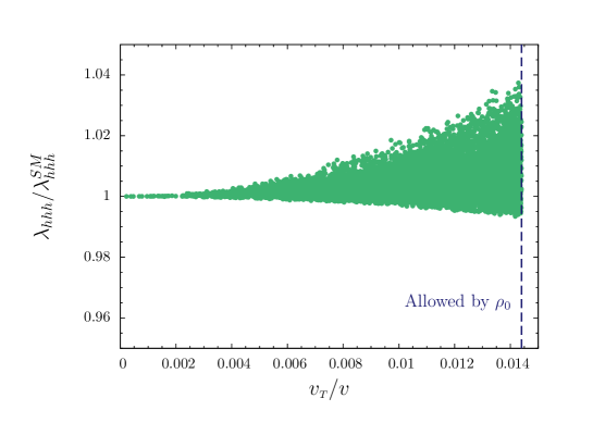
Figure 7: The modification of the trilinear Higgs self-coupling with respect to the SM as a function of $v_{\scriptscriptstyle T}/v$. For all points the minimum $(v_{\scriptscriptstyle H},v_{\scriptscriptstyle T})$ is the global one.

In Fig. 7 we show the results of our parameter scan. The trilinear Higgs self-coupling can only be modified by a few percent in the triplet model. This is a consequence of the small values for $v_{\scriptscriptstyle T}/v_{\scriptscriptstyle H}$ allowed by EW precision data.

As it can be inferred from the plot all points are stable at tree level. That can be understood as follows. In the neutral direction of $H$ the potential has stationary points in $\langle H\rangle=0$ and $\langle H\rangle=v_{\scriptscriptstyle H}/\sqrt{2}$. For $\langle H\rangle=v_{\scriptscriptstyle H}/\sqrt{2}$ the derivative of the potential with respect to the neutral component $\eta^{0}$ of $\Phi$ reads

$$\frac{\partial V}{\partial\eta_{0}}=\lambda_{2}\eta_{0}^{3}+\left(\mu_{2}^{2}+\frac{\lambda_{3}}{2}v_{\scriptscriptstyle H}^{2}\right)\eta_{0}-\frac{\mu_{4}}{2}v_{\scriptscriptstyle H}^{2}=0\,.$$ (64)

The discriminant of the cubic equation then reads

$$\Delta=-4\lambda_{2}\left(\mu_{2}^{2}+\frac{\lambda_{3}}{2}v_{\scriptscriptstyle H}^{2}\right)^{2}-\frac{27}{4}\lambda_{2}^{2}\,\mu_{4}^{2}\,v_{\scriptscriptstyle H}^{4}\,,$$ (65)

and $\Delta<0$ for all parameter sets due to the boundedness from below condition on $\lambda_{2}$ from eq. (59), hence there are no further stationary points with $\langle H\rangle=v_{\scriptscriptstyle H}/\sqrt{2}$ in $H$ direction. Note that for the singlet in Sect. 3.1, due to the $S^{3}$ term in the potential, the discriminant can also be larger than zero and hence other neutral minima can arise.

Two further stationary points are possible, namely ($\langle H\rangle=0$, $\langle\Phi\rangle=0$) and ($\langle H\rangle=0$, $|\langle\Phi\rangle|^{2}=-\mu_{2}^{2}/\lambda_{2}$). Since we always find $\mu_{2}^{2}>0$ in our scan the latter is not relevant here and ($\langle H\rangle=0$, $\langle\Phi\rangle=0$) must be a maximum by construction.

It is instructive to compare the previous results with the EFT limit where the triplet mass parameter is $\mu_{2}\gg v$. By integrating out the triplet in the $SU(2)_{L}$ limit via the equations of motion

$$\Phi^{\alpha}\simeq-\frac{\mu_{4}}{\mu_{2}^{2}+\lambda_{3}\left|H\right|^{2}}H^{\dagger}\sigma^{\alpha}H$$ (66)

the potential in the EFT reads

$$V_{\rm EFT}(H)\simeq-\frac{1}{2}\frac{\mu_{4}^{2}}{\mu_{2}^{2}+\lambda_{3}\left|H\right|^{2}}\left|H\right|^{4}=-\frac{\mu_{4}^{2}}{2\mu_{2}^{2}}\left|H\right|^{4}+\frac{\mu_{4}^{2}\lambda_{3}}{2\mu_{2}^{4}}\left|H\right|^{6}+\ldots\,,$$ (67)

where the expansion in the last term holds for Higgs fluctuations around the EW vev. The first term in Eq. (67) simply redefines the Higgs quartic coupling in the SM EFT, while the second one yields

$$c_{6}=\frac{\mu_{4}^{2}v_{\scriptscriptstyle H}^{2}\lambda_{3}}{2\mu_{2}^{4}}\,.$$ (68)

Always working in the $\mu_{2}\gg v$ limit, we can approximate the triplet vev as (cf. Eq. (92))

$$v_{\scriptscriptstyle T}\simeq\frac{\mu_{4}v_{\scriptscriptstyle H}^{2}}{2\mu_{2}^{2}}\,.$$ (69)

Hence, it is possible to recast the modified triple Higgs coupling as

$$\frac{\lambda_{hhh}}{\lambda^{\rm SM}_{hhh}}=1+\frac{2c_{6}v_{\scriptscriptstyle H}^{2}}{m^{2}_{h}}=1+\frac{4v_{\scriptscriptstyle T}^{2}\lambda_{3}}{m^{2}_{h}}\,,$$ (70)

where in the last step we have replaced $c_{6}$ in terms of $v_{\scriptscriptstyle T}$ (cf. Eqs. (68)–(69)). By plugging $v_{\scriptscriptstyle T}\lesssim 3.5$ GeV and $\lambda_{3}\in[-2\sqrt{0.1\times 4\pi},8\pi/\sqrt{3}]$ from perturbativity and vacuum stability (also, $\lambda_{1}\sim 0.1$ in order to reproduce the Higgs mass), we get $\lambda_{hhh}/\lambda^{\rm SM}_{hhh}\in[0.99,1.046]$, which fairly describes the range of deviations in Fig. 7.

A final comment on the other custodially violating cases is in order. By denoting the vev of the complex multiplet as $\left\langle\Phi\right\rangle=v_{\Phi}/\sqrt{2}$, the $2\sigma$-level bound from $\rho_{0}^{\rm(fit)}$ implies $v_{\Phi}\lesssim 1.7$, $2.9$, $1.0$ GeV, respectively for $\Phi=(1,3,1),(1,4,\frac{1}{2}),(1,4,\frac{3}{2})$. We hence expect suppressed contributions for the trilinear Higgs self-coupling, similarly to the triplet case.

3.3 Loop-induced trilinear Higgs self-coupling vs. vacuum stability

Loop modifications of the trilinear Higgs self-coupling are naturally expected to be smaller than tree-level ones. Nevertheless, we consider here the case where the new particles circulating in the loops are vector-like fermions, since we regain a clean correlation between the triple Higgs coupling and vacuum instability. This can be easily understood by looking at the loop of fermions contributing to the beta function of the Higgs self-coupling, which is basically the same diagram responsible for the radiative generation of the trilinear Higgs self-coupling in the broken phase after taking one Higgs to its vev (cf. Fig. 8).

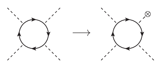
Figure 8: Schematic view of the connection between the beta-function of $\lambda$ and the loop-induced trilinear Higgs self-coupling via new fermions.

There are basically two qualitatively different possibilities: $i)$ non-SM-singlet fermions coupling to the Higgs and a SM fermion and $ii)$ SM-singlet fermions coupling to the Higgs and a lepton doublet. The former cases are bounded by other Higgs coupling measurements, which typically imply a very suppressed contribution to the trilinear Higgs self-coupling. The latter is more interesting, and correspond to the case of a right handed neutrino, which is largely unconstrained by other Higgs coupling measurements. A recent analysis was performed in Refs. [97, 98] in the context of a simplified $3+1$ Dirac neutrino model [97] and for the inverse seesaw model [98], finding deviations of the trilinear Higgs self-coupling with respect to the SM value up to $30\%$.

We want to show here the impact of vacuum stability in such a class of scenarios. Let us consider, for definiteness, the case of the inverse seesaw (similar conclusions apply to other neutrino mass models as well). We add to the SM field content three right-handed neutrinos and three gauge singlets $X$ with opposite lepton number, via the Lagrangian term

$$\mathcal{L}_{\rm ISS}=-Y_{\nu}\overline{L}\tilde{H}\nu_{R}-M_{R}\overline{\nu^{c}}X-\frac{1}{2}\mu_{X}\overline{X^{c}}X+\text{h.c.}\,,$$ (71)

where $\tilde{H}=i\sigma_{2}H^{*}$ and we suppressed family indices. We refer to Ref. [98] for the relevant notation and conventions. Taking, in particular, a diagonal Yukawa structure $Y_{\nu}=\left|y_{\nu}\right|I_{3}$ and a common mass scale for the three heavy neutrinos, $M_{R}=10$ TeV, one can asses the impact of the heavy neutrino states on the running of the Higgs self-coupling and hence on the stability of the Higgs effective potential $V_{\rm eff}(h)\approx 1/4\,\lambda_{\rm eff}(h)h^{4}$, where $\lambda_{\rm eff}(h)$ is approximated with the $\overline{\text{MS}}$ running coupling $\lambda(\mu=h)$. We use the two-loop beta functions for the SM couplings $(g_{1,2,3},y_{t},\lambda)$ and take into account the corrections due to $y_{\nu}$ at the one-loop level (and consistently we neglect the matching contributions of $y_{\nu}$ to $\lambda(M_{t})$). For simplicity, we also integrate in the heavy neutrinos at the common threshold $M_{R}=10$ TeV, while a more careful treatment should take into account intermediate EFTs when integrating in single neutrino thresholds (see e.g. Ref. [99]). Hence, in the case of a hierarchical heavy neutrino spectrum, our estimate of the largest energy scale until which the model can be consistently extrapolated should be conservatively rescaled starting from the heaviest threshold.

The results are displayed in Fig. 9 where we plot the value of $\lambda_{\rm eff}$ as a function of the renormalization scale $\mu$. The instability bound (red area) is computed by considering the probability of decay against quantum tunnelling in the modified Higgs potential integrated over the past light-cone (see e.g. [100, 101])

$$\mathcal{P}_{\rm{EW}}\simeq\left(\frac{\mu}{H_{0}}\right)^{4}e^{-\frac{8\pi^{2}}{3\left|\lambda_{\rm{eff}}(\mu)\right|}}\,,$$ (72)

where $H_{0}\simeq 10^{-42}$ GeV is the present Hubble constant. In particular, requiring $\mathcal{P}_{\rm{EW}}\simeq 1$ corresponds to

$$\left|\lambda_{\rm{eff}}(\mu)\right|\simeq\frac{0.064}{1+0.022\,\log_{10}\left(\frac{\mu}{1\ \rm{TeV}}\right)}\,,$$ (73)

which sets the instability bound for $\lambda_{\rm eff}<0$.

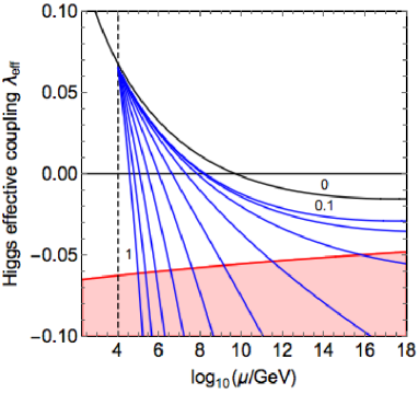
Figure 9: Running of $\lambda_{\rm eff}$ in the presence of a common heavy neutrino threshold $M_{R}=10$ TeV. Labels denote the the value of $y_{\nu}\in[0.1,1]$ with steps of $0.1$ (blue curves), while $y_{\nu}=0$ corresponds to the SM case (black curve). The instability bound is represented by the red-shaded area.

By increasing the value of $y_{\nu}$ between $0.1$ and $1$ (in steps of $0.1$), the instability scale dangerously approaches the heavy neutrino threshold (see Fig. 9), and in order to comply with the existence of the EW vacuum the model must be UV completed before entering the instability region. Using the approximate expression for $\Delta^{\rm BSM}_{\rm approx}\equiv\lambda_{hhh}/\lambda^{\rm SM}_{hhh}-1$ in Eq. (4.5) of [98] we obtain that $y_{\nu}=0.8$ corresponds to $\Delta^{\rm BSM}_{\rm approx}=0.1\ \%$. Hence, from Fig. 9 we read that modifications of the trilinear Higgs self-coupling above the per mil level require an UV completion within a few orders of magnitude from the scale where the heavy neutrinos are integrated in.

4 Conclusions

In this paper we have addressed the question on how much could the trilinear Higgs self-coupling deviate from its SM value. We first discussed in Sect. 2 theoretical constraints on Higgs self-couplings from a general standpoint by considering two main arguments: vacuum instability and pertubativity. We showed that the former cannot be reliably assessed in a model-independent way, due to the breakdown of the EFT in describing the global structure of the Higgs potential away from the EW minimum. In particular, we have explicitly shown that by augmenting the SM via an $\left|H\right|^{6}$ operator one can generate two type of instabilities, either at large field values $v\ll H\lesssim\Lambda$ or in $H=0$. In both cases, however, any reliable statement about the stability of the EW vacuum entails the knowledge of the full tower of effective operators, thus jeopardizing the connection with the Higgs self-couplings, whose leading order deviations are still governed by the $d=6$ operators.

On the other hand, it is possible to use perturbativity in order to set fairly model-independent limits on Higgs self-couplings. In Sect. 2.3 we have employed two different criteria, based either on the partial-wave unitarity of the $hh\to hh$ scattering or on the loop corrections of the tree-level vertices, in order to establish the perturbative domain of the Higgs self-couplings. Though being conceptually different, the two criteria agree well with each other both for the triple and the quartic Higgs coupling modifications: $|\lambda_{hhh}/\lambda_{hhh}^{SM}|\lesssim 6.5\,(6.0)$ and $|\lambda_{hhhh}/\lambda_{hhhh}^{SM}|\lesssim 65\,(68)$, with the first number corresponding to perturbative unitarity and the one in the bracket stemming from the loop-corrected vertex. Let us stress that indirect tests of the trilinear Higgs self-coupling either via single Higgs production [33, 34, 35] or EW precision tests [31, 30] and current measurements of non-resonant Higgs pair production [12] bound values of $\lambda_{hhh}$ which are, at the moment, well above our perturbativity limit $\left|\lambda_{hhh}/\lambda^{\rm SM}_{hhh}\right|\lesssim 6$.

In the second part of the paper (Sect. 3), we investigated the size of the trilinear Higgs self-coupling in explicit models. First, we identified the class of models potentially leading to the largest modifications in the trilinear Higgs self-coupling, namely scalar extensions featuring a tadpole operator of the type $\mathcal{O}_{\Phi}=\Phi f(H)$, where $f(H)$ is a string of Higgs fields. The list of new scalars coupling linearly to $H$ can be found in Table 1. They include both custodial symmetric (EW singlet and doublet) and custodial violating (EW triplets and quadruplets) scalar extensions. As two representative examples, we studied in detail the size of the trilinear Higgs self-coupling in the singlet and triplet extension, by taking into account constraints from EW precision tests, Higgs coupling measurements, direct searches for new scalars, vacuum stability and perturbativity. While in the singlet extension modifications of the trilinear Higgs coupling in the range $-1.5<\lambda_{hhh}/\lambda_{hhh}^{\rm SM}<8.7$ are still possible, for the custodially violating extensions, like e.g. the triplet case, only modifications up to few percent are allowed.

Remarkably, vacuum stability is not a crucial discriminant for limiting the size of the trilinear Higgs self-coupling in models featuring new scalars, where the intricate structure of the scalar potential allows for regions in parameter space where large quartics (at the boundary of perturbativity) can tame the instabilities triggered by the tadpole operators. On the other hand, we have also found circumstances where vacuum stability can be very relevant. That is the case in which the trilinear Higgs self-coupling is modified by loops of heavy fermions. In our explicit example in Sect. 3.3 we have considered the case of low-scale seesaw models, where the vacuum metastability bound can sizably reduce the allowed range for the trilinear Higgs self-coupling.

Acknowledgments. We thank Julien Baglio, Marco Nardecchia, Enrico Nardi, Michael Spira and Cédric Weiland for helpful discussions. RG is supported by a European Union COFUND/Durham Junior Research Fellowship under the EU grant number 609412. MS is supported in part by the European Commission through the “HiggsTools” Initial Training Network PITN-GA-2012-316704.

Appendix A Scalar potential parameters

In this appendix we collect some details on the scalar potential (e.g. tadpole equations and scalar spectrum) for the two models studied in Sect. 3.

A.1 Singlet

The scalar fields can be expanded around their vevs by

$$H=\frac{1}{\sqrt{2}}\left(\begin{array}[]{c}0\\ v_{\scriptscriptstyle H}+h\end{array}\right)\,,\qquad\Phi=(v_{\scriptscriptstyle S}+S)\,,$$ (74)

where we employed the unitary gauge for the Higgs doublet. The tadpole conditions can be written as

$$-\mu_{4}v_{\scriptscriptstyle S}-\frac{\lambda_{3}v_{\scriptscriptstyle S}^{2}}{2}-\mu_{1}^{2}-\lambda_{1}v_{\scriptscriptstyle H}^{2}=0\,,$$ (75)

$$-\frac{\mu_{4}v_{\scriptscriptstyle H}^{2}}{2}-\frac{1}{2}\lambda_{3}v_{\scriptscriptstyle H}^{2}v_{\scriptscriptstyle S}-\mu_{2}^{2}v_{\scriptscriptstyle S}-\lambda_{2}v_{\scriptscriptstyle S}^{3}-\mu_{3}v_{\scriptscriptstyle S}^{2}=0\,.$$ (76)

The first condition allows to replace $\mu_{1}^{2}$ in terms of $v_{\scriptscriptstyle H}$. The mass matrix in the real $(h,S)$ basis then reads

$$\mathcal{M}_{0}^{2}=\left(\begin{array}[]{cc}m_{\scriptscriptstyle{hh}}&m_{\scriptscriptstyle{hS}}\\ m_{\scriptscriptstyle{hS}}&m_{\scriptscriptstyle{SS}}\end{array}\right)\,,$$ (77)

with

$$m_{\scriptscriptstyle{hh}} =2v_{\scriptscriptstyle H}^{2}\lambda_{1}\,,$$ (78)

$$m_{\scriptscriptstyle{hS}} =v_{\scriptscriptstyle H}\left(\mu_{4}+\lambda_{3}v_{\scriptscriptstyle S}\right)\,,$$ (79)

$$m_{\scriptscriptstyle{SS}} =\mu_{2}^{2}+\frac{1}{2}\left(\lambda_{3}v_{\scriptscriptstyle H}^{2}+6v_{\scriptscriptstyle S}^{2}\lambda_{2}+4v_{\scriptscriptstyle S}\mu_{3}\right)\,.$$ (80)

The mass matrix is diagonalized by rotating

$$\left(\begin{array}[]{c}h_{1}\\ h_{2}\end{array}\right)=\left(\begin{array}[]{cc}\cos\theta&-\sin\theta\\ \sin\theta&\cos\theta\end{array}\right)\left(\begin{array}[]{c}h\\ S\end{array}\right)\,,$$ (81)

with

$$\tan 2\theta=\frac{2m_{\scriptscriptstyle{hS}}}{m_{\scriptscriptstyle{SS}}-m_{\scriptscriptstyle{hh}}}\,,$$ (82)

and mass eigenvalues

$$m_{1,2}^{2} =\frac{1}{2}\left(m_{\scriptscriptstyle{hh}}+m_{\scriptscriptstyle{SS}}\mp\sqrt{4m_{\scriptscriptstyle{hS}}^{2}+(m_{\scriptscriptstyle{hh}}-m_{\scriptscriptstyle{SS}})^{2}}\right)$$

$$=\frac{1}{2}\left(m_{\scriptscriptstyle{hh}}+m_{\scriptscriptstyle{SS}}\pm(m_{\scriptscriptstyle{hh}}-m_{\scriptscriptstyle{SS}})\frac{1}{\cos 2\theta}\right)\,.$$ (83)

Expressing the couplings of the potential in terms of the parameters used for the scan, we find

$$\mu_{1}^{2} =-\frac{1}{4}\left[\left(-2\lambda_{3}v_{\scriptscriptstyle S}^{2}+m_{1}^{2}+m_{2}^{2}\right)+\cos(2\theta)(m_{1}^{2}-m_{2}^{2})-2\frac{v_{\scriptscriptstyle S}}{v_{\scriptscriptstyle H}}\sin(2\theta)(m_{1}^{2}-m_{2}^{2})\right]\,,$$ (84)

$$\mu_{2}^{2} =\frac{1}{2}\left[\left(\lambda_{3}v_{\scriptscriptstyle H}^{2}-m_{1}^{2}-m_{2}^{2}+2\lambda_{2}v_{\scriptscriptstyle S}^{2}\right)+\frac{v_{\scriptscriptstyle H}}{v_{\scriptscriptstyle S}}\sin(2\theta)(m_{1}^{2}-m_{2}^{2})+\cos(2\theta)(m_{1}^{2}-m_{2}^{2})\right]\,,$$ (85)

$$\mu_{3} =\frac{1}{2v_{\scriptscriptstyle S}}\left[\left(m_{1}^{2}+m_{2}^{2}-\lambda_{3}v_{\scriptscriptstyle H}^{2}-4\lambda_{2}v_{\scriptscriptstyle S}^{2}\right)-\frac{1}{2}\frac{v_{\scriptscriptstyle H}}{v_{\scriptscriptstyle S}}\sin(2\theta)(m_{1}^{2}-m_{2}^{2})-\cos(2\theta)(m_{1}^{2}-m_{2}^{2})\right]\,,$$ (86)

$$\mu_{4} =\frac{\sin(2\theta)(m_{2}^{2}-m_{1}^{2})-2\lambda_{3}v_{\scriptscriptstyle H}v_{\scriptscriptstyle S}}{2v_{\scriptscriptstyle H}}\,,$$ (87)

$$\lambda_{1} =\frac{\cos(2\theta)(m_{1}^{2}-m_{2}^{2})+m_{1}^{2}+m_{2}^{2}}{4v_{\scriptscriptstyle H}^{2}}\,.$$ (88)

A.2 Triplet

The scalar fields can be expanded around their charge-preserving vevs via

$$H=\left(\begin{array}[]{c}\phi^{+}\\ \frac{1}{\sqrt{2}}\left(v_{\scriptscriptstyle H}+h^{0}+iG^{0}\right)\end{array}\right)\,,\hskip 28.45274pt\Phi=\left(\begin{array}[]{c}\eta_{1}\\ \eta_{2}\\ v_{\scriptscriptstyle T}+\eta_{0}\end{array}\right)\,,$$ (90)

where the charged eigenstates for $\Phi$ are defined as $\eta^{\pm}=\tfrac{1}{\sqrt{2}}\left(\eta_{1}\mp i\eta_{2}\right)$. The tadpole conditions can be written as

$$0 =\mu_{1}^{2}+\lambda_{1}v_{\scriptscriptstyle H}^{2}+\frac{\lambda_{3}}{2}v_{\scriptscriptstyle T}^{2}-\mu_{4}v_{\scriptscriptstyle T}\,,$$ (91)

$$0 =v_{\scriptscriptstyle T}\left(\mu_{2}^{2}+\lambda_{2}v_{\scriptscriptstyle T}^{2}+\frac{\lambda_{3}}{2}v_{\scriptscriptstyle H}^{2}\right)-\frac{\mu_{4}}{2}v_{\scriptscriptstyle H}^{2}\,.$$ (92)

For $v_{\scriptscriptstyle T}=0$ there is no doublet/triplet mixing and Eq. (92) implies $\mu_{4}=0$, which corresponds to the custodial symmetric tree-level relation $\rho=1$. From now on we will assume $v_{\scriptscriptstyle T}\neq 0$. By evaluating the second derivatives of the scalar potential and after imposing the stationary Eqs. (91)–(91), we find the following scalar spectrum:

• Charged scalars: in the complex $(\phi^{+},\eta^{+})$ basis

  $$\mathcal{M}^{2}_{+}=\left(\begin{array}[]{cc}2\mu_{4}v_{\scriptscriptstyle T}&\mu_{4}v_{\scriptscriptstyle H}\\ \mu_{4}v_{\scriptscriptstyle H}&\frac{\mu_{4}v_{\scriptscriptstyle H}^{2}}{2v_{\scriptscriptstyle T}}\end{array}\right)\,,$$ (93)

  which features a null eigenvalue, corresponding to the Goldstone boson $G^{+}$ eaten by the $W$, and a massive state $h^{\pm}$ with mass

  $$m^{2}_{h^{\pm}}=\frac{\mu_{4}\left(v_{\scriptscriptstyle H}^{2}+4v_{\scriptscriptstyle T}^{2}\right)}{2v_{\scriptscriptstyle T}}\,.$$ (94)

• Neutral pseudo-scalar: $G^{0}$, corresponding to the Goldstone boson eaten by the $Z$.

• Neutral scalars: in the real $(h^{0},\eta^{0})$ basis

  $$\mathcal{M}_{0}^{2}=\left(\begin{array}[]{cc}m_{\scriptscriptstyle{hh}}&m_{\scriptscriptstyle{h\eta}}\\ m_{\scriptscriptstyle{h\eta}}&m_{\scriptscriptstyle{\eta\eta}}\end{array}\right)\,,$$ (95)

  with

  $$m_{\scriptscriptstyle{hh}} =2\lambda_{1}v_{\scriptscriptstyle H}^{2}\,,$$ (96)

  $$m_{\scriptscriptstyle{h\eta}} =v\left(\lambda_{3}v_{\scriptscriptstyle T}-\mu_{4}\right)\,,$$ (97)

  $$m_{\scriptscriptstyle{\eta\eta}} =2\lambda_{2}v_{\scriptscriptstyle T}^{2}+\frac{\mu_{4}v_{\scriptscriptstyle H}^{2}}{2v_{\scriptscriptstyle T}}\,.$$ (98)

  The mass eigenstates are obtained via the rotation

  $$\left(\begin{array}[]{c}h_{1}\\ h_{2}\end{array}\right)=\left(\begin{array}[]{cc}\cos\theta&-\sin\theta\\ \sin\theta&\cos\theta\end{array}\right)\left(\begin{array}[]{c}h^{0}\\ \eta^{0}\end{array}\right)\,,$$ (99)

  with

  $$\tan 2\theta=\frac{2v_{\scriptscriptstyle H}\left(\lambda_{3}v_{\scriptscriptstyle T}-\mu_{4}\right)}{2\lambda_{2}v_{\scriptscriptstyle T}^{2}+\frac{\mu_{4}v_{\scriptscriptstyle H}^{2}}{2v_{\scriptscriptstyle T}}-2\lambda_{1}v_{\scriptscriptstyle H}^{2}}\,,$$ (100)

  and mass eigenvalues

  $$m_{1,2}^{2} =\frac{1}{2}\left(m_{\scriptscriptstyle{hh}}+m_{\scriptscriptstyle{\eta\eta}}\mp\sqrt{4m_{\scriptscriptstyle{h\eta}}^{2}+(m_{\scriptscriptstyle{hh}}-m_{\scriptscriptstyle{\eta\eta}})^{2}}\right)$$

  $$=\frac{1}{2}\left(m_{\scriptscriptstyle{hh}}+m_{\scriptscriptstyle{\eta\eta}}\pm(m_{\scriptscriptstyle{hh}}-m_{\scriptscriptstyle{\eta\eta}})\frac{1}{\cos 2\theta}\right)\,.$$ (101)

Moreover, the $W$ boson mass is given by

$$m^{2}_{W}=\frac{g^{2}}{4}\left(v_{\scriptscriptstyle H}^{2}+4v_{\scriptscriptstyle T}^{2}\right)\,,$$ (102)

which fixes $v^{2}=(246.2\ \text{GeV})^{2}=v_{\scriptscriptstyle H}^{2}+4v_{\scriptscriptstyle T}^{2}$, while EW precision tests set a bound on the custodial-breaking vev $v_{\scriptscriptstyle T}\lesssim 3.5$ GeV. Summarising, an independent set of parameters can be chosen as:

$$v_{\scriptscriptstyle H}=\sqrt{v^{2}-4v_{\scriptscriptstyle T}^{2}}\,,\;\;\;v_{\scriptscriptstyle T}<3.55\ \text{GeV}\,,\;\;\;m_{1}=125\text{ GeV}\,,\;\;\;m_{2}\,,\;\;\;m_{h^{\pm}}\,,\;\;\;\theta\,.$$ (103)

Note, however, that in Sect. 3.2 we scan over $\lambda_{2}$ instead of $m_{2}$. For completeness, we report here the potential parameters expressed in terms of those in Eq. (103)

$$\mu_{4} =\frac{2m^{2}_{h^{\pm}}v_{\scriptscriptstyle T}}{v_{\scriptscriptstyle H}^{2}+4v_{\scriptscriptstyle T}^{2}}\,,$$ (104)

$$\lambda_{1} =\frac{m_{1}^{2}+m_{2}^{2}+(m_{1}^{2}-m_{2}^{2})\cos 2\theta}{4v_{\scriptscriptstyle H}^{2}}\,,$$ (105)

$$\lambda_{2} =\frac{(m_{1}^{2}+m_{2}^{2})v_{\scriptscriptstyle T}-\mu_{4}v_{\scriptscriptstyle H}^{2}+(m_{2}^{2}-m_{1}^{2})v_{\scriptscriptstyle T}\cos 2\theta}{4v_{\scriptscriptstyle T}^{3}}\,,$$ (106)

$$\lambda_{3} =\frac{2\mu_{4}v_{\scriptscriptstyle H}+(m_{2}^{2}-m_{1}^{2})\sin 2\theta}{2v_{\scriptscriptstyle H}v_{\scriptscriptstyle T}}\,.$$ (107)

References

- [1] ATLAS Collaboration, G. Aad et al., “Observation of a new particle in the search for the Standard Model Higgs boson with the ATLAS detector at the LHC,” Phys. Lett. B716 (2012) 1–29, arXiv:1207.7214 [hep-ex].
- [2] CMS Collaboration, S. Chatrchyan et al., “Observation of a new boson at a mass of 125 GeV with the CMS experiment at the LHC,” Phys. Lett. B716 (2012) 30–61, arXiv:1207.7235 [hep-ex].
- [3] F. Englert and R. Brout, “Broken Symmetry and the Mass of Gauge Vector Mesons,” Phys. Rev. Lett. 13 (1964) 321–323.
- [4] P. W. Higgs, “Broken Symmetries and the Masses of Gauge Bosons,” Phys. Rev. Lett. 13 (1964) 508–509.
- [5] F. R. Klinkhamer and N. S. Manton, “A Saddle Point Solution in the Weinberg-Salam Theory,” Phys. Rev. D30 (1984) 2212.
- [6] M. Spannowsky and C. Tamarit, “Sphalerons in composite and non-standard Higgs models,” Phys. Rev. D95 no. 1, (2017) 015006, arXiv:1611.05466 [hep-ph].
- [7] ATLAS Collaboration, “Search for Higgs boson pair production in the final state using pp collision data at TeV with the ATLAS detector,” Tech. Rep. ATLAS-CONF-2016-004, CERN, Geneva, Mar, 2016. http://cds.cern.ch/record/2138949.
- [8] ATLAS Collaboration, M. Aaboud et al., “Search for pair production of Higgs bosons in the final state using proton–proton collisions at TeV with the ATLAS detector,” Phys. Rev. D94 no. 5, (2016) 052002, arXiv:1606.04782 [hep-ex].
- [9] ATLAS Collaboration, “Search for Higgs boson pair production in the final state of () using 13.3 fb-1 of collision data recorded at 13 TeV with the ATLAS detector,” Tech. Rep. ATLAS-CONF-2016-071, CERN, Geneva, Aug, 2016. http://cds.cern.ch/record/2206222.
- [10] CMS Collaboration, “Search for non-resonant pair production of Higgs bosons in the final state with 13 TeV CMS data,” Tech. Rep. CMS-PAS-HIG-16-026, CERN, Geneva, 2016. https://cds.cern.ch/record/2209572.
- [11] CMS Collaboration, “Search for pair production of Higgs bosons in the two tau leptons and two bottom quarks final state using proton-proton collisions at ,” Tech. Rep. CMS-PAS-HIG-17-002, CERN, Geneva, 2017. https://cds.cern.ch/record/2256096.
- [12] CMS Collaboration, “Search for resonant and non-resonant Higgs boson pair production in the final state at ,” Tech. Rep. CMS-PAS-HIG-17-006, CERN, Geneva, 2017. https://cds.cern.ch/record/2257068.
- [13] A. Djouadi, W. Kilian, M. Muhlleitner, and P. M. Zerwas, “Testing Higgs selfcouplings at e+ e- linear colliders,” Eur. Phys. J. C10 (1999) 27–43, arXiv:hep-ph/9903229 [hep-ph].
- [14] A. Djouadi, W. Kilian, M. Muhlleitner, and P. M. Zerwas, “Production of neutral Higgs boson pairs at LHC,” Eur. Phys. J. C10 (1999) 45–49, arXiv:hep-ph/9904287 [hep-ph].
- [15] U. Baur, T. Plehn, and D. L. Rainwater, “Determining the Higgs boson selfcoupling at hadron colliders,” Phys. Rev. D67 (2003) 033003, arXiv:hep-ph/0211224 [hep-ph].
- [16] U. Baur, T. Plehn, and D. L. Rainwater, “Probing the Higgs selfcoupling at hadron colliders using rare decays,” Phys. Rev. D69 (2004) 053004, arXiv:hep-ph/0310056 [hep-ph].
- [17] M. J. Dolan, C. Englert, and M. Spannowsky, “Higgs self-coupling measurements at the LHC,” JHEP 10 (2012) 112, arXiv:1206.5001 [hep-ph].
- [18] J. Baglio, A. Djouadi, R. Gröber, M. M. Mühlleitner, J. Quevillon, and M. Spira, “The measurement of the Higgs self-coupling at the LHC: theoretical status,” JHEP 04 (2013) 151, arXiv:1212.5581 [hep-ph].
- [19] A. J. Barr, M. J. Dolan, C. Englert, and M. Spannowsky, “Di-Higgs final states augMT2ed – selecting events at the high luminosity LHC,” Phys. Lett. B728 (2014) 308–313, arXiv:1309.6318 [hep-ph].
- [20] M. J. Dolan, C. Englert, N. Greiner, and M. Spannowsky, “Further on up the road: production at the LHC,” Phys. Rev. Lett. 112 (2014) 101802, arXiv:1310.1084 [hep-ph].
- [21] A. Papaefstathiou, L. L. Yang, and J. Zurita, “Higgs boson pair production at the LHC in the channel,” Phys. Rev. D87 no. 1, (2013) 011301, arXiv:1209.1489 [hep-ph].
- [22] F. Goertz, A. Papaefstathiou, L. L. Yang, and J. Zurita, “Higgs Boson self-coupling measurements using ratios of cross sections,” JHEP 06 (2013) 016, arXiv:1301.3492 [hep-ph].
- [23] D. E. Ferreira de Lima, A. Papaefstathiou, and M. Spannowsky, “Standard model Higgs boson pair production in the ( )( ) final state,” JHEP 08 (2014) 030, arXiv:1404.7139 [hep-ph].
- [24] C. Englert, F. Krauss, M. Spannowsky, and J. Thompson, “Di-Higgs phenomenology in : The forgotten channel,” Phys. Lett. B743 (2015) 93–97, arXiv:1409.8074 [hep-ph].
- [25] T. Liu and H. Zhang, “Measuring Di-Higgs Physics via the Channel,” arXiv:1410.1855 [hep-ph].
- [26] F. Goertz, A. Papaefstathiou, L. L. Yang, and J. Zurita, “Higgs boson pair production in the D=6 extension of the SM,” JHEP 04 (2015) 167, arXiv:1410.3471 [hep-ph].
- [27] A. Azatov, R. Contino, G. Panico, and M. Son, “Effective field theory analysis of double Higgs boson production via gluon fusion,” Phys. Rev. D92 no. 3, (2015) 035001, arXiv:1502.00539 [hep-ph].
- [28] A. Carvalho, M. Dall’Osso, T. Dorigo, F. Goertz, C. A. Gottardo, and M. Tosi, “Higgs Pair Production: Choosing Benchmarks With Cluster Analysis,” JHEP 04 (2016) 126, arXiv:1507.02245 [hep-ph].
- [29] J. K. Behr, D. Bortoletto, J. A. Frost, N. P. Hartland, C. Issever, and J. Rojo, “Boosting Higgs pair production in the final state with multivariate techniques,” Eur. Phys. J. C76 no. 7, (2016) 386, arXiv:1512.08928 [hep-ph].
- [30] G. Degrassi, M. Fedele, and P. P. Giardino, “Constraints on the trilinear Higgs self coupling from precision observables,” arXiv:1702.01737 [hep-ph].
- [31] G. D. Kribs, A. Maier, H. Rzehak, M. Spannowsky, and P. Waite, “Electroweak oblique parameters as a probe of the trilinear Higgs self-interaction,” arXiv:1702.07678 [hep-ph].
- [32] M. McCullough, “An Indirect Model-Dependent Probe of the Higgs Self-Coupling,” Phys. Rev. D90 no. 1, (2014) 015001, arXiv:1312.3322 [hep-ph]. [Erratum: Phys. Rev.D92,no.3,039903(2015)].
- [33] M. Gorbahn and U. Haisch, “Indirect probes of the trilinear Higgs coupling: and ,” JHEP 10 (2016) 094, arXiv:1607.03773 [hep-ph].
- [34] G. Degrassi, P. P. Giardino, F. Maltoni, and D. Pagani, “Probing the Higgs self coupling via single Higgs production at the LHC,” JHEP 12 (2016) 080, arXiv:1607.04251 [hep-ph].
- [35] W. Bizon, M. Gorbahn, U. Haisch, and G. Zanderighi, “Constraints on the trilinear Higgs coupling from vector boson fusion and associated Higgs production at the LHC,” arXiv:1610.05771 [hep-ph].
- [36] S. Di Vita, C. Grojean, G. Panico, M. Riembau, and T. Vantalon, “A global view on the Higgs self-coupling,” arXiv:1704.01953 [hep-ph].
- [37] T. Plehn and M. Rauch, “The quartic higgs coupling at hadron colliders,” Phys. Rev. D72 (2005) 053008, arXiv:hep-ph/0507321 [hep-ph].
- [38] T. Binoth, S. Karg, N. Kauer, and R. Ruckl, “Multi-Higgs boson production in the Standard Model and beyond,” Phys. Rev. D74 (2006) 113008, arXiv:hep-ph/0608057 [hep-ph].
- [39] CLIC Physics Working Group Collaboration, E. Accomando et al., “Physics at the CLIC multi-TeV linear collider,” in Proceedings, 11th International Conference on Hadron spectroscopy (Hadron 2005): Rio de Janeiro, Brazil, August 21-26, 2005. 2004. arXiv:hep-ph/0412251 [hep-ph]. http://weblib.cern.ch/abstract?CERN-2004-005.
- [40] C. P. Burgess, V. Di Clemente, and J. R. Espinosa, “Effective operators and vacuum instability as heralds of new physics,” JHEP 01 (2002) 041, arXiv:hep-ph/0201160 [hep-ph].
- [41] J. M. Cornwall, D. N. Levin, and G. Tiktopoulos, “Derivation of Gauge Invariance from High-Energy Unitarity Bounds on the s Matrix,” Phys. Rev. D10 (1974) 1145. [Erratum: Phys. Rev.D11,972(1975)].
- [42] B. W. Lee, C. Quigg, and H. B. Thacker, “The Strength of Weak Interactions at Very High-Energies and the Higgs Boson Mass,” Phys. Rev. Lett. 38 (1977) 883–885.
- [43] V. Barger, T. Han, P. Langacker, B. McElrath, and P. Zerwas, “Effects of genuine dimension-six Higgs operators,” Phys. Rev. D67 (2003) 115001, arXiv:hep-ph/0301097 [hep-ph].
- [44] R. Contino, M. Ghezzi, C. Grojean, M. Mühlleitner, and M. Spira, “Effective Lagrangian for a light Higgs-like scalar,” JHEP 07 (2013) 035, arXiv:1303.3876 [hep-ph].
- [45] A. Pomarol, “Higgs Physics,” in Proceedings, 2014 European School of High-Energy Physics (ESHEP 2014): Garderen, The Netherlands, June 18 - July 01 2014, pp. 59–77. 2016. arXiv:1412.4410 [hep-ph]. http://inspirehep.net/record/1334375/files/arXiv:1412.4410.pdf.
- [46] G. F. Giudice, C. Grojean, A. Pomarol, and R. Rattazzi, “The Strongly-Interacting Light Higgs,” JHEP 06 (2007) 045, arXiv:hep-ph/0703164 [hep-ph].
- [47] A. Schuessler and D. Zeppenfeld, “Unitarity constraints on MSSM trilinear couplings,” in SUSY 2007 Proceedings, 15th International Conference on Supersymmetry and Unification of Fundamental Interactions, July 26 - August 1, 2007, Karlsruhe, Germany, pp. 236–239. 2007. arXiv:0710.5175 [hep-ph]. http://www.susy07.uni-karlsruhe.de/Proceedings/proceedings/susy07.pdf.
- [48] L. Di Luzio, J. F. Kamenik, and M. Nardecchia, “Implications of perturbative unitarity for scalar di-boson resonance searches at LHC,” Eur. Phys. J. C77 no. 1, (2017) 30, arXiv:1604.05746 [hep-ph].
- [49] B. W. Lee, C. Quigg, and H. B. Thacker, “Weak Interactions at Very High-Energies: The Role of the Higgs Boson Mass,” Phys. Rev. D16 (1977) 1519.
- [50] M. Luscher and P. Weisz, “Is There a Strong Interaction Sector in the Standard Lattice Higgs Model?,” Phys. Lett. B212 (1988) 472–478.
- [51] H. H. Patel, “Package-X: A Mathematica package for the analytic calculation of one-loop integrals,” Comput. Phys. Commun. 197 (2015) 276–290, arXiv:1503.01469 [hep-ph].
- [52] F. Goertz, J. F. Kamenik, A. Katz, and M. Nardecchia, “Indirect Constraints on the Scalar Di-Photon Resonance at the LHC,” JHEP 05 (2016) 187, arXiv:1512.08500 [hep-ph].
- [53] M. J. Dolan, C. Englert, and M. Spannowsky, “New Physics in LHC Higgs boson pair production,” Phys. Rev. D87 no. 5, (2013) 055002, arXiv:1210.8166 [hep-ph].
- [54] J. M. No and M. Ramsey-Musolf, “Probing the Higgs Portal at the LHC Through Resonant di-Higgs Production,” Phys. Rev. D89 no. 9, (2014) 095031, arXiv:1310.6035 [hep-ph].
- [55] C.-Y. Chen, S. Dawson, and I. M. Lewis, “Exploring resonant di-Higgs boson production in the Higgs singlet model,” Phys. Rev. D91 no. 3, (2015) 035015, arXiv:1410.5488 [hep-ph].
- [56] V. Martín Lozano, J. M. Moreno, and C. B. Park, “Resonant Higgs boson pair production in the decay channel,” JHEP 08 (2015) 004, arXiv:1501.03799 [hep-ph].
- [57] S. I. Godunov, A. N. Rozanov, M. I. Vysotsky, and E. V. Zhemchugov, “Extending the Higgs sector: an extra singlet,” Eur. Phys. J. C76 (2016) 1, arXiv:1503.01618 [hep-ph].
- [58] S. Banerjee, B. Batell, and M. Spannowsky, “Invisible decays in Higgs boson pair production,” Phys. Rev. D95 no. 3, (2017) 035009, arXiv:1608.08601 [hep-ph].
- [59] T. Huang, J. M. No, L. Pernié, M. Ramsey-Musolf, A. Safonov, M. Spannowsky, and P. Winslow, “Resonant Di-Higgs Production in the Channel: Probing the Electroweak Phase Transition at the LHC,” arXiv:1701.04442 [hep-ph].
- [60] I. M. Lewis and M. Sullivan, “Benchmarks for the Singlet Extended Standard Model at the LHC,” arXiv:1701.08774 [hep-ph].
- [61] S. Dawson, A. Ismail, and I. Low, “What’s in the loop? The anatomy of double Higgs production,” Phys. Rev. D91 no. 11, (2015) 115008, arXiv:1504.05596 [hep-ph].
- [62] R. Gröber, M. Mühlleitner, and M. Spira, “Signs of Composite Higgs Pair Production at Next-to-Leading Order,” JHEP 06 (2016) 080, arXiv:1602.05851 [hep-ph].
- [63] A. Agostini, G. Degrassi, R. Gröber, and P. Slavich, “NLO-QCD corrections to Higgs pair production in the MSSM,” JHEP 04 (2016) 106, arXiv:1601.03671 [hep-ph].
- [64] F. del Aguila, J. de Blas, and M. Perez-Victoria, “Electroweak Limits on General New Vector Bosons,” JHEP 09 (2010) 033, arXiv:1005.3998 [hep-ph].
- [65] C. Biggio, M. Bordone, L. Di Luzio, and G. Ridolfi, “Massive vectors and loop observables: the case,” JHEP 10 (2016) 002, arXiv:1607.07621 [hep-ph].
- [66] J. de Blas, M. Chala, M. Perez-Victoria, and J. Santiago, “Observable Effects of General New Scalar Particles,” JHEP 04 (2015) 078, arXiv:1412.8480 [hep-ph].
- [67] L. Di Luzio, R. Gröber, J. F. Kamenik, and M. Nardecchia, “Accidental matter at the LHC,” JHEP 07 (2015) 074, arXiv:1504.00359 [hep-ph].
- [68] Y. Jiang and M. Trott, “On the non-minimal character of the SMEFT,” arXiv:1612.02040 [hep-ph].
- [69] R. S. Gupta, H. Rzehak, and J. D. Wells, “How well do we need to measure the Higgs boson mass and self-coupling?,” Phys. Rev. D88 (2013) 055024, arXiv:1305.6397 [hep-ph].
- [70] A. Efrati and Y. Nir, “What if ,” arXiv:1401.0935 [hep-ph].
- [71] D. López-Val and T. Robens, “ and the W-boson mass in the singlet extension of the standard model,” Phys. Rev. D90 (2014) 114018, arXiv:1406.1043 [hep-ph].
- [72] ATLAS Collaboration, G. Aad et al., “Constraints on new phenomena via Higgs boson couplings and invisible decays with the ATLAS detector,” JHEP 11 (2015) 206, arXiv:1509.00672 [hep-ex].
- [73] T. Robens and T. Stefaniak, “LHC Benchmark Scenarios for the Real Higgs Singlet Extension of the Standard Model,” Eur. Phys. J. C76 no. 5, (2016) 268, arXiv:1601.07880 [hep-ph].
- [74] J. R. Espinosa, T. Konstandin, and F. Riva, “Strong Electroweak Phase Transitions in the Standard Model with a Singlet,” Nucl. Phys. B854 (2012) 592–630, arXiv:1107.5441 [hep-ph].
- [75] J. E. Camargo-Molina, B. O’Leary, W. Porod, and F. Staub, “: A Tool For Finding The Global Minima Of One-Loop Effective Potentials With Many Scalars,” Eur. Phys. J. C73 no. 10, (2013) 2588, arXiv:1307.1477 [hep-ph].
- [76] J. E. Camargo-Molina, B. Garbrecht, B. O’Leary, W. Porod, and F. Staub, “Constraining the Natural MSSM through tunneling to color-breaking vacua at zero and non-zero temperature,” Phys. Lett. B737 (2014) 156–161, arXiv:1405.7376 [hep-ph].
- [77] F. Staub, “SARAH,” arXiv:0806.0538 [hep-ph].
- [78] F. Staub, “From Superpotential to Model Files for FeynArts and CalcHep/CompHep,” Comput. Phys. Commun. 181 (2010) 1077–1086, arXiv:0909.2863 [hep-ph].
- [79] F. Staub, “Automatic Calculation of supersymmetric Renormalization Group Equations and Self Energies,” Comput. Phys. Commun. 182 (2011) 808–833, arXiv:1002.0840 [hep-ph].
- [80] F. Staub, “SARAH 3.2: Dirac Gauginos, UFO output, and more,” Comput. Phys. Commun. 184 (2013) 1792–1809, arXiv:1207.0906 [hep-ph].
- [81] F. Staub, “SARAH 4 : A tool for (not only SUSY) model builders,” Comput. Phys. Commun. 185 (2014) 1773–1790, arXiv:1309.7223 [hep-ph].
- [82] D. Buttazzo, F. Sala, and A. Tesi, “Singlet-like Higgs bosons at present and future colliders,” JHEP 11 (2015) 158, arXiv:1505.05488 [hep-ph].
- [83] S. Kanemura, M. Kikuchi, and K. Yagyu, “One-loop corrections to the Higgs self-couplings in the singlet extension,” Nucl. Phys. B917 (2017) 154–177, arXiv:1608.01582 [hep-ph].
- [84] J. E. Camargo-Molina, A. P. Morais, R. Pasechnik, M. O. P. Sampaio, and J. Wessén, “All one-loop scalar vertices in the effective potential approach,” JHEP 08 (2016) 073, arXiv:1606.07069 [hep-ph].
- [85] S. Kanemura, Y. Okada, E. Senaha, and C. P. Yuan, “Higgs coupling constants as a probe of new physics,” Phys. Rev. D70 (2004) 115002, arXiv:hep-ph/0408364 [hep-ph].
- [86] J. Bernon, J. F. Gunion, H. E. Haber, Y. Jiang, and S. Kraml, “Scrutinizing the alignment limit in two-Higgs-doublet models. II. mH=125 GeV,” Phys. Rev. D93 no. 3, (2016) 035027, arXiv:1511.03682 [hep-ph].
- [87] J. Baglio, O. Eberhardt, U. Nierste, and M. Wiebusch, “Benchmarks for Higgs Pair Production and Heavy Higgs boson Searches in the Two-Higgs-Doublet Model of Type II,” Phys. Rev. D90 no. 1, (2014) 015008, arXiv:1403.1264 [hep-ph].
- [88] I. F. Ginzburg, “Triple Higgs coupling in the most general 2HDM at SM-like scenario,” Eur. Phys. J. C77 no. 1, (2017) 9, arXiv:1510.08270 [hep-ph].
- [89] M.-C. Chen, S. Dawson, and T. Krupovnickas, “Higgs triplets and limits from precision measurements,” Phys. Rev. D74 (2006) 035001, arXiv:hep-ph/0604102 [hep-ph].
- [90] B. W. Lynn and E. Nardi, “Radiative corrections in unconstrained SU(2) x U(1) and the top mass problem,” Nucl. Phys. B381 (1992) 467–500.
- [91] T. Blank and W. Hollik, “Precision observables in SU(2) x U(1) models with an additional Higgs triplet,” Nucl. Phys. B514 (1998) 113–134, arXiv:hep-ph/9703392 [hep-ph].
- [92] Particle Data Group Collaboration, C. Patrignani et al., “Review of Particle Physics,” Chin. Phys. C40 no. 10, (2016) 100001.
- [93] P. Bechtle, O. Brein, S. Heinemeyer, G. Weiglein, and K. E. Williams, “HiggsBounds: Confronting Arbitrary Higgs Sectors with Exclusion Bounds from LEP and the Tevatron,” Comput. Phys. Commun. 181 (2010) 138–167, arXiv:0811.4169 [hep-ph].
- [94] P. Bechtle et al., “HiggsBounds-4: Improved Tests of Extended Higgs Sectors against Exclusion Bounds from LEP, the Tevatron and the LHC,” Eur. Phys. J. C74 (2014) 2693, arXiv:1311.0055 [hep-ph].
- [95] P. Bechtle, S. Heinemeyer, O. Stal, T. Stefaniak, and G. Weiglein, “Applying Exclusion Likelihoods from LHC Searches to Extended Higgs Sectors,” arXiv:1507.06706 [hep-ph].
- [96] N. Khan, “Exploring Hyperchargeless Higgs Triplet Model up to the Planck Scale,” arXiv:1610.03178 [hep-ph].
- [97] J. Baglio and C. Weiland, “Heavy neutrino impact on the triple Higgs coupling,” Phys. Rev. D94 no. 1, (2016) 013002, arXiv:1603.00879 [hep-ph].
- [98] J. Baglio and C. Weiland, “The triple Higgs coupling: A new probe of low-scale seesaw models,” arXiv:1612.06403 [hep-ph].
- [99] L. Delle Rose, C. Marzo, and A. Urbano, “On the stability of the electroweak vacuum in the presence of low-scale seesaw models,” JHEP 12 (2015) 050, arXiv:1506.03360 [hep-ph].
- [100] G. Isidori, G. Ridolfi, and A. Strumia, “On the metastability of the standard model vacuum,” Nucl. Phys. B609 (2001) 387–409, arXiv:hep-ph/0104016 [hep-ph].
- [101] L. Di Luzio, G. Isidori, and G. Ridolfi, “Stability of the electroweak ground state in the Standard Model and its extensions,” Phys. Lett. B753 (2016) 150–160, arXiv:1509.05028 [hep-ph].