DAWSON-HEP 5, CUMQ/HEP 193
Top and bottom partners, Higgs boson on the brane, and the tth signal

Abstract

Current LHC results indicate a possible enhancement in the production of Higgs bosons in association with top quarks ($t\bar{t}h$) over the Standard Model (SM) expectations, suggesting an increase in the top Yukawa coupling. To explain these results, we study the effect of adding to the SM a small set of vector-like partners of the top and bottom quarks with masses of order $\sim 1$ TeV. We consider Yukawa coupling matrices with vanishing determinant and show that then, Higgs production through gluon fusion is not affected by deviations in the top quark Yukawa coupling, and in fact depends only on deviations in the bottom quark Yukawa coupling. We call this scenario the Brane Higgs Limit, as it can emerge naturally in models of warped extra-dimensions with all matter fields in the bulk, except the Higgs (although it could also occur in 4D scenarios with vector-like quarks and special flavor symmetries forcing the vanishing of the Yukawa determinants). We show that the scenario is highly predictive for all Higgs production/decay modes, making it easily falsifiable, maybe even at the LHC RUN 2 with higher luminosity.

I Introduction

RUN 1 of the LHC culminated in the discovery of the Higgs boson at 125 GeV. After the Higgs discovery, the most important question is, naturally, where is the new physics beyond the Standard Model (SM), and how will it manifest itself? Minimal additions to the SM could be revealed as an unexpected excess in dileptons, $W^{+}W^{-}$, $ZZ$, diphotons, $t\bar{t}$ or $b\bar{b}$, indicating the presence of a new boson resonance. More involved new physics could also appear as missing energy, or any other signals indicating the presence of supersymmetry or extra-dimensions or other exotic particles. But also, new physics could manifest itself indirectly. In particular it could affect the production cross section and decay widths of the Higgs boson, expected to be measured with increased precision during the current RUN2 of the LHC. There are already several promising signals in the RUN 1 data indicating possible deviations from the SM expectations. In particular, both ATLAS and CMS report a possible increase in the signal strength of the $t{\bar{t}}h$ associated production in the LHC data. Of particular interest from RUN 1 at CMS and ATLAS are the same-sign dilepton (SS2$l$) and trilepton ($3l$) signals coming from leptonic Higgs decays in the associated $t{\bar{t}}h$ production events. The best fit signal strengths are found to be $\mu_{SS2l}=5.3^{+2.1}_{-1.8}$ and $\mu_{3l}=3.1^{+2.4}_{-2.0}$ at CMS Khachatryan:2014qaa , and $\mu_{SS2l}=2.8^{+2.1}_{-1.9}$ and $\mu_{3l}=2.8^{+2.2}_{-1.8}$ at ATLAS Aad:2015iha . These leptonic excesses are associated to the channels $tt(h\to WW^{*})$, $tt(h\to ZZ^{*})$ and $tt(h\to\tau\tau)$ where one of the tops decays leptonically. Within the preliminary results of RUN 2 in those same leptonic channels, both ATLAS and CMS still report excesses with, for example, $\mu_{SS2l}=1.9^{+0.9}_{-0.8}$ at CMS CMS:2016vqb and $\mu_{SS2l}=4.0^{+2.1}_{-1.7}$ at ATLAS ATLAS:2016awy . The most recent preliminary results reported by CMS in the $t{\bar{t}}h$ associated production searches make use of an integrated luminosity of 35.9 fb^-1 and seem to show mixed results. In the leptonic channels ($W^{+}W^{-}$ and $ZZ$ channels) they still show an enhancement of $1.5\pm 0.5$ times the SM prediction, with an observed (expected) significance of 3.3 $\sigma$ (2.5 $\sigma$) obtained from combining these results with the 2015 data CMS:2017vru . On the other hand in the $h\to\tau\tau$ decay channel search, a slight suppression of $0.72^{+0.62}_{-0.53}$ times the SM prediction is found, with an observed (expected) significance of $1.4\sigma$ ($1.8\sigma$) CMS:2017lgc . Note that, unlike the $W^{+}W^{-}$ and $ZZ$ decays, this last signal is sensitive to both the top-Higgs Yukawa and the $\tau$-Higgs Yukawa couplings, and thus enhancements or suppressions are possible as long as there are variations in either the top quark and the $\tau$ lepton Yukawa couplings.

All measurements are still hindered by having few events so far, but nevertheless, should these tantalizing signals survive more precise measurements at higher luminosities, they will provide the much awaited signals for new physics. We summarize relevant production and decay channels in Table 1 with the overall combinations obtained by the ATLAS and CMS collaborations, for the signal strengths associated to each Higgs production and decay channels.

Production Mode	Channel	RUN-1 Khachatryan:2016vau	Production Mode	Channel	ATLAS RUN-2	CMS RUN-2
$ggh$	$\gamma\gamma$	$1.1^{+0.23}_{-0.22}$	$ggh$	$\gamma\gamma$	$0.62^{+0.30}_{-0.29}$ ATLAS:2016hru	$0.77^{+0.25}_{-0.23}$ CMS:2016ixj
	$WW^{*}$	$0.84^{+0.17}_{-0.17}$		$WW^{*}$	-	-
	$ZZ^{*}$	$1.13^{+0.34}_{-0.31}$		$ZZ^{*}$	$1.34^{+0.39}_{-0.33}$ ATLAS:2016hru	$0.96^{+0.44}_{-0.33}$ CMS:2016ilx
$t{\bar{t}}h$	$\gamma\gamma$	$2.2^{+1.6}_{-1.3}$	$t{\bar{t}}h$	$\gamma\gamma,b{\bar{b}},$ leptons	$1.8^{+0.7}_{-0.7}$ ATLAS:2016axz	-
	$b{\bar{b}}$	$1.15^{+0.99}_{-0.94}$		$WW^{\star},ZZ^{\star},\tau^{+}\tau^{-}$		$2.0^{+0.8}_{-0.7}$ CMS:2016vqb
	$WW^{\star}$	$5.0^{+2.6}_{-2.2}$

Table 1: Higgs signal strengths used in our analysis, from $ggh$ and $t{\bar{t}}h$ production modes measured at the LHC from RUN 1 (combined $\sqrt{s}=7$ and $8$ TeV results) and RUN 2 ($\sqrt{s}=13$ TeV).

One possibility to explain the SS2$l$ excess, is that it could be due to a modified Higgs coupling to the SM top quark, resulting in an enhanced $t{\bar{t}}$ ($h\to$ multileptons) production. A simple explanation put forward to explain this latest possible signal of physics beyond the SM has been to invoke the presence of vector-like quarks Angelescu:2015kga . Previous studies have adopted an effective theory approach, involving generic couplings and mixings with the third generation quarks, by which they induce modifications of the Yukawa couplings of the top and bottom quarks. The scenario has been put forward to explain deviations from SM expectations in the forward-backward asymmetry in $b$ decays $A_{\rm FB}^{b}$ and the enhancement of the $pp\to t{\bar{t}}h$ cross section at the LHC. Mixing with the additional states in the bottom sector allows for a sufficiently large increase of the $Zb_{R}{\bar{b}}_{R}$ coupling to explain the forward-backward anomaly, as well as imply new effects in Higgs phenomenology Choudhury:2001hs ; vectorlike . The mixing could provide a strong enhancement of the $t{\bar{t}}h$ Yukawa coupling, which would explain an increase of the cross section at the LHC. In this scenario, rates for the loop-induced processes stay SM-like due to either small vector-like contributions or compensating effects between fermion mixing and loop contributions. For this to be a viable scenario, vector-like quark masses of order 1-2 TeV are required, still safe from the LHC lower limits on their masses, $m_{\rm VLQ}\mathrel{\raise 1.29167pt\hbox{$>$\kern-7.5pt\lower 4.30554pt\hbox{$\sim$}}}800$ GeV Aad:2015mba .

In Section II of this article, we first revisit the SM augmented by the addition of one vector-like quark doublet and two singlets (one top-like and one bottom-like) and review the mixing with the third family of quarks. In Sec. II.1, we then show that there is a specific region of parameter space where large corrections to the top Yukawa coupling (caused by contributions from the new vector-like quarks) do not cause large corrections to the radiative coupling of the Higgs and gluons. We show that in that limit, Higgs signal strengths can be simply parametrized in terms of four variables only, related to the top and bottom quark shifts in Yukawa couplings, which we analyze in Sec. II.2, in terms of the parameters of the model. Based on these results, we present simple predictions between signal strength in Higgs production (through gluon fusion and $t{\bar{t}}h$) and decays into $\gamma\gamma,\,WW$ and $ZZ$, in Sec. II.3. As seen in that subsection, large regions of parameter space are excluded by both theoretical considerations and experimental constraints. Finally, in Sec III we describe how to reproduce our scenario within the conventional Randall Sundrum model and then summarize our findings in Sec. IV.

II Top and Bottom Mirrors: a doublet and two singlets

The simple scenario that we wish to consider contains the usual SM gauge groups and matter fields, with the addition of a vector-like quark $SU(2)$ doublet and two vector-like quarks $SU(2)$ singlets, one with up-type gauge charge and another with down-type gauge charge. They can be regarded as top or bottom partners as we will consider that their Yukawa couplings are large. As we will show in the next section, this structure can appear naturally in models of warped extra dimensions with the Higgs localized near the TeV brane, and with fermions in the bulk. The presence of brane kinetic terms can lower significantly the mass of some of the heavy Kaluza Klein fermions Frank:2016vtv . The rest of the KK fields decouple due to their heavy masses , giving rise to something similar to the simple setup considered here. We denote $q^{0}_{L}\equiv\begin{pmatrix}t^{0}_{L}\\ b^{0}_{L}\end{pmatrix}$ as the SM third generation doublet, and $t^{0}_{R}$ as the SM right handed top. Using similar notation we define $Q_{L,R}\equiv\begin{pmatrix}Q^{t}_{L,R}\\ Q^{b}_{L,R}\end{pmatrix}$ as the new vector-like quark doublet, $T_{R,L}$ as the new vector-like up-type quark singlet, and $B_{L,R}$ as the new vector-like down-type singlet.

In principle we should also consider the mixings with the $up$ and $charm$ quarks, and $down$ and $strange$ quarks of the SM when writing down the most general Yukawa couplings in the up and down sectors. Without any additional assumption or theory input, we should write down the most general Yukawa couplings between SM quarks and the new vector-like quarks, leading to a $5\times 5$ fermion mass matrices. In models of warped extra dimensions with bulk fermions, the couplings between up or charm and heavy fermions are suppressed by factors of order $\sqrt{m_{f}/m_{t}}$ with respect to the couplings to the top, which are of order 1, and so we will just neglect those terms, leading to a much simpler $3\times 3$ fermion mass matrix (and similarly in the down sector with the bottom quark).

The mass and interaction Lagrangian in the top sector, including its Yukawa couplings with the SM-like Higgs doublet $\tilde{H}$ can be then written as

$${\cal L}_{mass} = Y_{t}^{0}\ \overline{q}_{L}\tilde{H}t_{R}+Y_{qT}\ \overline{q}_{L}\tilde{H}T_{R}+Y_{Qt}\ \overline{Q}_{L}\tilde{H}t_{R}+Y_{1}\overline{Q}_{L}\tilde{H}T_{R}+Y_{2}\overline{Q}_{R}\tilde{H}T_{L}$$ (1)

$$+M_{Q}\overline{Q}_{L}Q_{R}+M_{T}\overline{T}_{L}T_{R},$$

with a similar expression for the bottom sector. After electroweak symmetry breaking, the Yukawa couplings induce off-diagonal terms into the fermion mass matrix. In the basis defined by the vectors $(\overline{q}_{L},\overline{Q}_{L},\overline{T}_{L})$ and $(t_{R},Q_{R},T_{R})$ we can write the heavy quarks mass matrix as

$${\bf M_{t}}=\begin{pmatrix}vY_{t}^{0}&0&vY_{qT}\\ vY_{Qt}&M_{Q}&vY^{t}_{1}\\ 0&vY^{t}_{2}&M_{T}\end{pmatrix}.$$ (2)

where, in general, all entries are complex and where $v$ is the Higgs vacuum expectation value (VEV). We can also express the bottom sector heavy quark mass matrix as

$${\bf M_{b}}=\begin{pmatrix}vY_{b}^{0}&0&vY_{qB}\\ vY_{Qb}&M_{Q}&vY^{b}_{1}\\ 0&vY^{b}_{2}&M_{B}\end{pmatrix}~{},$$ (3)

where again all entries can be complex and the value of $M_{Q}$ is the same in both ${\bf M_{t}}$ and ${\bf M_{b}}$. The associated top and bottom Yukawa coupling matrices are

$${\bf\tilde{Y}_{t}}=\begin{pmatrix}Y_{t}^{0}&0&Y_{qT}\\ Y_{Qt}&0&Y^{t}_{1}\\ 0&Y^{t}_{2}&0\end{pmatrix}\ \ \ {\rm and}\ \ \ \ {\bf\tilde{Y}_{b}}=\begin{pmatrix}Y_{b}^{0}&0&Y_{qB}\\ Y_{Qb}&0&Y^{b}_{1}\\ 0&Y^{b}_{2}&0\end{pmatrix}.$$ (4)

The mass matrices ${\bf M_{t}}$ and ${\bf M_{b}}$ are diagonalized by bi-unitary transformations, ${\bf V_{t}}^{\dagger}_{L}{\bf M_{t}}{\bf V_{t}}_{R}={\bf M_{t}}^{diag}$, and ${\bf V_{b}}^{\dagger}_{L}{\bf M_{b}}{\bf V_{b}}_{R}={\bf M_{b}}^{diag}$. At the same time, the Higgs Yukawa couplings are obtained after transforming the Yukawa matrices into the physical basis, ${\bf V_{t}}^{\dagger}_{L}{\bf\tilde{Y}_{t}}{\bf V_{t}}_{R}={\bf Y_{t}}^{phys}$ and ${\bf V_{b}}^{\dagger}_{L}{\bf\tilde{Y}_{b}}{\bf V_{b}}_{R}={\bf Y_{b}}^{phys}$.

II.1 Higgs Production in the Brane Higgs Limit

In the physical basis, the top quark mass and the top Yukawa coupling (the first entries in the physical mass matrix and the physical Yukawa matrix) are not related anymore by the SM relationship $m_{t}^{phys}=vy_{t}^{SM}$ Azatov:2009na (with $v$ normalized to $v=174$ GeV for simplicity). The same goes for the bottom quark, and we thus define the shifts, $\delta y_{t}$ and $\delta y_{t}$, between the SM and the physical Yukawa couplings, due to the diagonalization, as

$$y^{phys}_{t}=y^{SM}_{t}-\delta y_{t}$$ (5)

and

$$y^{phys}_{b}=y^{SM}_{b}-\delta y_{b}.$$ (6)

Later we will give an approximate expression of these shifts in terms of the model parameters of Eqs. (2) and (3). But before that, we consider the radiative coupling of the Higgs to gluons. This coupling depends on the physical Yukawa couplings $y_{nn}$ of all the fermions running in the loop and on their physical masses $m_{n}$. The real and imaginary parts of the couplings (the scalar and pseudoscalar parts) contribute to the cross section through different loop functions, $A^{S}_{1/2}$ and $A^{P}_{1/2}$, as they generate the two operators $hG_{\mu\nu}G^{\mu\nu}$ and $hG_{\mu\nu}\tilde{G}^{\mu\nu}$.

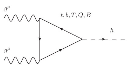
Figure 1: Feynman diagram for the production cross section $gg\to h$ in a setup with new vector-like fermions $Q$, $T$ and $B$.

The cross section, depicted in Fig. 1, is

$$\sigma_{gg\rightarrow h}={\alpha_{s}^{2}m_{h}^{2}\over 576\pi}\left[|c^{S}_{ggh}|^{2}+|c^{P}_{ggh}|^{2}\right]\ \delta(s-m_{h}^{2})$$ (7)

where

$$c^{S}_{ggh}=\sum^{3}_{n=1}\hbox{Re}\left({\frac{y_{nn}}{m_{n}}}\right)A^{S}_{1/2}(\tau_{f})\hskip 17.07182pt{\rm and}\hskip 17.07182ptc^{P}_{ggh}=\sum^{3}_{n=1}{\rm Im}\left(\frac{y_{nn}}{m_{n}}\right)A^{P}_{1/2}(\tau_{f})$$ (8)

with $\ \tau=m^{2}_{h}/4m^{2}_{n}\$ and with the loop functions $A^{S}_{1/2}(\tau)$ and $A^{P}_{1/2}(\tau)$ as defined in Gunion:1989we . Note that we use a normalization of the loop functions such that for very heavy quarks with masses $m_{n}$ much greater than the Higgs mass $m_{h}$ (i.e. when $\tau$ is very small) they behave asymptotically as $\displaystyle\lim_{\tau\to 0}A^{S}_{1/2}=1\hskip 5.69046pt\mbox{and}\hskip 5.69046pt\lim_{\tau\to 0}A^{P}_{1/2}=3/2.$ On the other hand, for light quarks (all the SM quarks except top and to some extent, bottom), the loop functions essentially vanish since $\displaystyle\lim_{\tau\to\infty}A^{S}_{1/2}=\lim_{\tau\to\infty}A^{P}_{1/2}=0$, and we thus neglect contributions from the light SM quarks and consider only the effect of the top, the bottom and the four remaining physical heavy quarks.

The amplitudes $c^{S}_{ggh}$ and $c^{P}_{ggh}$ can then be written in terms of traces involving the fermion mass and Yukawa matrices involving top and vector-like up-quarks, and bottom and any vector-like down quarks, ${\bf M}_{i}$ and ${\bf Y}_{i}$ with $i=t,b$, so that we obtain

$$c^{S}_{ggh}=\sum_{n}\hbox{Re}\left({\frac{y^{u}_{nn}}{m^{u}_{n}}}\right)+\sum_{n}\hbox{Re}\left({\frac{y^{d}_{nn}}{m^{d}_{n}}}\right)-\hbox{Re}\left({\frac{y_{b}}{m_{b}}}\right)+\hbox{Re}\left({\frac{y_{b}}{m_{b}}}\right)A^{S}_{1/2}(\tau_{b})$$ (9)

where we have added and subtracted the bottom quark loop contribution in order to keep the dependence in $A_{1/2}(\tau_{b})$, and with a similar expression holding for $c^{P}_{ggh}$. We evaluate exactly the sums in the top and bottom sectors and find

$$\sum_{n}\left({\frac{y^{u}_{nn}}{m^{u}_{n}}}\right) = \frac{1}{v}\frac{1+3\varepsilon_{Q_{t}}\varepsilon_{T}\frac{|Y^{t}_{2}|}{|Y_{t}^{0}|}e^{i\theta^{t}_{2}}\left(1-e^{i\theta^{t}_{1}}\frac{|Y^{t}_{1}||Y_{t}^{0}|}{|Y_{Qt}||Y_{qT}|}\right)}{1+\varepsilon_{Q_{t}}\varepsilon_{T}\frac{|Y^{t}_{2}|}{|Y_{t}^{0}|}e^{i\theta^{t}_{2}}\left(1-e^{i\theta^{t}_{1}}\frac{|Y^{t}_{1}||Y_{t}^{0}|}{|Y_{Qt}||Y_{qT}|}\right)},$$ (10)

and

$$\sum_{n}\left({\frac{y^{d}_{nn}}{m^{d}_{n}}}\right) = \frac{1}{v}\frac{1+3\varepsilon_{Q_{b}}\varepsilon_{B}\frac{|Y^{b}_{2}|}{|Y_{b}^{0}|}e^{i\theta^{b}_{2}}\left(1-e^{i\theta^{b}_{1}}\frac{|Y^{b}_{1}||Y_{b}^{0}|}{|Y_{Qb}||Y_{qB}|}\right)}{1+\varepsilon_{Q_{b}}\varepsilon_{B}\frac{|Y^{b}_{2}|}{|Y_{b}^{0}|}e^{i\theta^{b}_{2}}\left(1-e^{i\theta^{b}_{1}}\frac{|Y^{b}_{1}||Y_{b}^{0}|}{|Y_{Qb}||Y_{qB}|}\right)},$$ (11)

where we have defined the small parameters $\displaystyle\varepsilon_{T}=\frac{v|Y_{qT}|}{|M_{T}|}\$, $\displaystyle\varepsilon_{B}=\frac{v|Y_{qB}|}{|M_{B}|}\$, $\displaystyle\ \varepsilon_{Q_{t}}=\frac{v|Y_{Qt}|}{|M_{Q}|}\$ and $\displaystyle\ \varepsilon_{Q_{b}}=\frac{v|Y_{Qb}|}{|M_{Q}|}\$, and with the relative phases $\theta^{i}_{1}$ and $\theta^{i}_{2}$ defined as $\theta^{t}_{1}=Arg\left(\frac{Y_{t}^{0}Y^{t}_{1}}{Y_{Qt}Y_{qT}}\right)$ and $\theta^{t}_{2}=Arg\left(\frac{Y_{qT}Y_{Qt}Y^{t}_{2}}{M_{T}M_{Q}Y^{0}_{t}}\right)$, with similar definitions for $\theta_{1}^{b}$ and $\theta_{2}^{b}$. In the SM limit, the expression in Eq. (9) should tend to $\sim\displaystyle\frac{1}{v}(1+A_{1/2}^{S}(\tau_{b}))$, and so if one wished to limit the contribution coming from the top partners to Higgs production (in gluon fusion), we must reduce/eliminate these corrections. We note the following observations.

• Of course for heavier and heavier vector-like fermions, the parameters $\varepsilon_{i}$ become more and more suppressed, and thus we can smoothly recover the SM limit, but the new physics effect will decouple from everywhere else (and in particular the top Yukawa quark will also tend to its SM value).

• It might also be possible to reduce the couplings $|Y^{t}_{2}|$ or $|Y^{b}_{2}|$ , but then this will also affect the physical top or bottom Yukawa couplings shifts, and in particular no enhancement in the top quark Yukawa coupling will be possible (although suppression might still be possible), as we will show later.

• Another interesting possibility would be to set the overall phase of the correction term in Eqs. (10) or (11) to be $\pi/2$ so that the real part vanishes (in general, we expect that the real part would dominate the overall corrections, at least for $\varepsilon_{i}<1$). This possibility might limit the amount of enhancement in the top Yukawa coupling, since that correction also depends on the phase $\theta_{2}$. Again when we compute the approximate expression of the Yukawa couplings shift, we will see that the phase $\theta_{2}$ should be close to $0$ to yield an enhancement in the top Yukawa coupling.

• In our considerations, we will impose a seemingly contrived constraint on the model parameters, which we call the Brane Higgs Limit, such that

  $$\det{\bf\tilde{Y}_{t}}=\det{\bf\tilde{Y}_{b}}=0,$$ (12)

  with the matrices ${\bf\tilde{Y}_{t}}$ and ${\bf\tilde{Y}_{b}}$ defined in Eq. (4). This constraint implies that

  $$Y^{t}_{2}\left(1-e^{i\theta_{1}}\frac{|Y^{t}_{1}||Y_{t}^{0}|}{|Y_{Qt}||Y_{qT}|}\right)=0,$$ (13)

  and thus ensures that the top sector contribution to Higgs production, given in Eq. (10), gives the same result as the SM top quark contribution to the same process. The vanishing determinant condition could come from a specific flavor structure in the Yukawa matrix, emerging for example from democratic textures, etc. We will show in the next section that the flavor structure required can also be obtained in models of extra-dimensions, so that the cancellation in Eq. (13) is satisfied exactly if the scenario arises out of the usual Randall-Sundrum warped extra-dimensional scenario with matter fields in bulk. It is necessary, though, that the Higgs be sufficiently localized towards the brane and that the KK modes of the top quark (and bottom quark) be much lighter than the KK partners of the up and charm quarks (and the down and strange quarks). We will then refer to the vector-like partners of the top and bottom quarks throughout as KK partners, and we return to this scenario in Sec. III.

Therefore we work in the Brane Higgs Limit of the general parameter space. In the down sector, we also have $Y^{b}_{2}\left(1-e^{i\theta^{b}_{1}}\frac{|Y^{b}_{1}||Y_{b}^{0}|}{|Y_{Qb}||Y_{qB}|}\right)=0$, so that we have

$$\sum_{n}\left({\frac{y^{u}_{nn}}{m^{u}_{n}}}\right)\ =\ \sum_{n}\left({\frac{y^{d}_{nn}}{m^{d}_{n}}}\right)\ =\ \frac{1}{v}\,.$$ (14)

This means that now we can write the $ggh$ couplings as

$$c^{S}_{ggh} = \frac{1}{v}\left(1+A^{S}_{1/2}(\tau_{b})\right)+\hbox{Re}\left(\frac{\delta y_{b}}{m_{b}}\right)\left(1-A^{S}_{1/2}(\tau_{b})\right)\,,$$ (15)

$${\rm and}\hskip 85.35826pt$$

$$c^{P}_{ggh} = {\rm Im}\left(\frac{\delta y_{b}}{m_{b}}\right)\left(\frac{3}{2}-A^{P}_{1/2}(\tau_{b})\right),\ \ \ \ \ \$$ (16)

where we have used the definitions of the Yukawa coupling shifts in Eqs. (5) and (6). Evaluating the values for the bottom quark loop functions $A^{S,P}_{1/2}(\tau_{b})$ we obtain

$$\frac{\sigma_{gg\rightarrow h}}{\sigma^{SM}_{gg\rightarrow h}}=\frac{\Gamma_{h\rightarrow gg}}{\Gamma^{SM}_{h\rightarrow gg}}=(1+\Delta_{gg})~{},$$ (17)

where the correction term is

$$\Delta_{gg}=2.13v\left(\hbox{Re}\frac{\delta y_{b}}{m_{b}}\right)+1.13v^{2}\left(\hbox{Re}\frac{\delta y_{b}}{m_{b}}\right)^{2}+2.51v^{2}\left({\rm Im}\frac{\delta y_{b}}{m_{b}}\right)^{2}.$$ (18)

This result links in a simple and nontrivial way Higgs production through gluon fusion to the bottom quark Yukawa coupling (or more precisely to its relative shift $v\delta y_{b}/m_{b}$). In a similar fashion we can also obtain the correction to the Higgs decay into $\gamma\gamma$ in the Brane Higgs Limit, since the fermion loop is the same as the gluon fusion loop (although there is an additional $W$ loop contribution in this case). We obtain

$$\frac{\Gamma_{h\to\gamma\gamma}}{\Gamma^{SM}_{h\to\gamma\gamma}}=(1+\Delta_{\gamma\gamma})\,,$$ (19)

with

$$\Delta_{\gamma\gamma} = -0.14v\left(\hbox{Re}\frac{\delta y_{b}}{m_{b}}\right)+0.005v^{2}\left(\hbox{Re}\frac{\delta y_{b}}{m_{b}}\right)^{2}+0.01v^{2}\left({\rm Im}\frac{\delta y_{b}}{m_{b}}\right)^{2},$$ (20)

and where we took the SM loop contributions to be $|c_{\gamma\gamma}|=|-7A_{1}(\tau_{W})+16/9A^{S}_{1/2}(\tau_{t})+4/9A^{S}_{1/2}(\tau_{b})|\simeq 6.53$, with the W-loop function $A_{1}(\tau_{W})$ Gunion:1989we and the fermion loop function $A^{S}_{1/2}(\tau_{f})$ normalized so that $\lim_{\tau\to 0}A_{i}(\tau)=1$. Finally, from Eqs.(5) and (6) we can now write

$$\frac{\sigma_{pp\rightarrow tth}}{\sigma^{SM}_{pp\rightarrow tth}}=\left|\frac{y_{t}}{y_{SM}}\right|^{2}=(1+\Delta_{tt})\ \ \ \ \ \ \ {\rm and}\ \ \ \ \ \ \ \frac{\Gamma_{h\to b}}{\Gamma^{SM}_{h\to bb}}=\left|\frac{y_{b}}{y_{SM}}\right|^{2}=(1+\Delta_{bb}),\ \ \ \$$ (21)

where

$$\Delta_{tt}=-2v\hbox{Re}\left(\frac{\delta y_{t}}{m_{t}}\right)+v^{2}\left|\frac{\delta y_{t}}{m_{t}}\right|^{2}\ \ \ \ {\rm and}\ \ \ \ \Delta_{bb}=-2v\hbox{Re}\left(\frac{\delta y_{b}}{m_{b}}\right)+v^{2}\left|\frac{\delta y_{b}}{m_{b}}\right|^{2}\,.$$ (22)

We are interested in studying the dependence on the Yukawa shifts $\delta y_{t}$ and $\delta y_{b}$ of the signal strengths

$$\displaystyle\mu^{ii}_{ggh}=\frac{\sigma(gg\to h)Br(h\to ii)}{\sigma_{SM}(gg\to h)Br^{SM}(h\to ii)}\ =\frac{\sigma(gg\to h)}{\sigma_{SM}(gg\to h)}\ \frac{\Gamma(h\to ii)\ }{\Gamma_{SM}(h\to ii)}\ \frac{\Gamma_{SM}^{tot}(h)}{\Gamma^{tot}(h)},$$ (23)

with a similar expression for $\mu^{ii}_{t\bar{t}h}$ (and using the small width approximation). In these expressions, the ratio of total Higgs widths can be written as

$$\frac{\Gamma_{SM}^{tot}(h)}{\Gamma^{tot}(h)} = \frac{1}{\left(1+Br^{SM}_{h\to bb}\Delta_{bb}+Br^{SM}_{h\to gg}\Delta_{gg}+Br^{SM}_{h\to\gamma\gamma}\Delta_{\gamma\gamma}\right)}\ \ \ \,,$$ (24)

where, taking into account numerical values for the SM Higgs branching ratios, gives simply

$$\frac{\Gamma_{SM}^{tot}(h)}{\Gamma^{tot}(h)} \simeq \frac{1}{1+0.58\Delta_{bb}+0.086\Delta_{gg}}~{},$$ (25)

and where we have dropped the dependence in $\Delta_{\gamma\gamma}$ as it is much suppressed.

With all these ingredients, we find the $t{\bar{t}}h$ production-and-decay strengths

$$\mu^{VV}_{t{\bar{t}}h} = \frac{(1+\Delta_{tt})}{(1+0.58\Delta_{bb}+0.086\Delta_{gg})}\,,$$ (26)

$$\mu^{bb}_{t{\bar{t}}h} = \mu^{VV}_{t{\bar{t}}h}(1+\Delta_{bb})\,,$$ (27)

$$\mu^{\gamma\gamma}_{t{\bar{t}}h} = \mu^{VV}_{t{\bar{t}}h}(1+\Delta_{\gamma\gamma})~{},$$ (28)

as well as the $ggh$ strengths

$$\mu^{VV}_{ggh} = \frac{(1+\Delta_{gg})}{(1+0.58\Delta_{bb}+0.086\Delta_{gg})}\,,$$ (29)

$$\mu^{\gamma\gamma}_{ggh} = \mu^{VV}_{ggh}(1+\Delta_{\gamma\gamma})~{},$$ (30)

with the corrections $\Delta_{ii}$ depending only on top or bottom quark Yukawa coupling shifts

$$\Delta_{tt} = -2v\hbox{Re}\left(\frac{\delta y_{t}}{m_{t}}\right)+v^{2}\left|\frac{\delta y_{t}}{m_{t}}\right|^{2}\ \$$ (31)

$$\Delta_{bb} = -2v\hbox{Re}\left(\frac{\delta y_{b}}{m_{b}}\right)+v^{2}\left|\frac{\delta y_{b}}{m_{b}}\right|^{2}$$ (32)

$$\Delta_{gg} = 2.13v\left(\hbox{Re}\frac{\delta y_{b}}{m_{b}}\right)+1.13v^{2}\left(\hbox{Re}\frac{\delta y_{b}}{m_{b}}\right)^{2}+2.51v^{2}\left({\rm Im}\frac{\delta y_{b}}{m_{b}}\right)^{2}$$ (33)

$$\Delta_{\gamma\gamma} = -0.14v\left(\hbox{Re}\frac{\delta y_{b}}{m_{b}}\right)+0.005v^{2}\left(\hbox{Re}\frac{\delta y_{b}}{m_{b}}\right)^{2}+0.01v^{2}\left({\rm Im}\frac{\delta y_{b}}{m_{b}}\right)^{2}~{}.$$ (34)

II.2 Yukawa Coupling Shifts

As indicated before, the mass matrices ${\bf M_{t}}$ and ${\bf M_{b}}$ from Eqs. (2) and (3) are diagonalized by bi-unitary transformations, ${\bf V_{t}}^{\dagger}_{L}{\bf M_{t}}{\bf V_{t}}_{R}={\bf M_{t}}^{diag}$, and ${\bf V_{b}}^{\dagger}_{L}{\bf M_{b}}{\bf V_{b}}_{R}={\bf M_{b}}^{diag}$. In order to obtain simple analytical expressions for the Yukawa couplings emerging after the diagonalization, we expand the unitary matrices ${\bf V_{t,b}}_{L}$ and ${\bf V_{t,b}}_{R}$ in powers of $\varepsilon\sim v/M$, where $v$ is the Higgs VEV and $M$ represents the vector-like masses $M_{Q}$, $M_{T}$ or $M_{B}$.

In this approximation we can obtain the lightest mass eigenvalues (the top quark and the bottom quark masses) as well as the physical $t{\bar{t}}h$ Yukawa coupling and the $b{\bar{b}}h$ Yukawa coupling.

This yields the relative deviation between the physical Yukawa couplings $y_{t}^{phys}$ and $y_{b}^{phys}$, and the SM Yukawa couplings, defined as $y_{t}^{SM}=m_{t}^{phys}/v$ and $y_{b}^{SM}=m_{b}^{phys}/v$. In terms of the mass matrix parameters from Eqs. (2) and (3), we obtain

$$\frac{\delta y_{t}}{y_{t}^{SM}}\ =\ \varepsilon_{T}^{2}+\varepsilon_{Q_{t}}^{2}-2\varepsilon_{T}\varepsilon_{Q_{t}}\frac{|Y_{2}|}{|Y_{t}^{0}|}e^{i\theta^{t}_{2}}\ +\ {\cal O}(\varepsilon^{4}),$$ (35)

and similarly for the bottom quark

$$\frac{\delta y_{b}}{y_{b}^{SM}}=\ \varepsilon_{B}^{2}+\varepsilon_{Q_{b}}^{2}-2\varepsilon_{B}\varepsilon_{Q_{b}}\frac{|Y^{b}_{2}|}{|Y_{b}^{0}|}e^{i\theta^{b}_{2}}\ +\ {\cal O}(\varepsilon^{4}).$$ (36)

As previously, $\displaystyle\varepsilon_{T}=\frac{v|Y_{qT}|}{|M_{T}|}\$, $\displaystyle\varepsilon_{B}=\frac{v|Y_{qB}|}{|M_{B}|}\$, $\displaystyle\ \varepsilon_{Q_{t}}=\frac{v|Y_{Qt}|}{|M_{Q}|}\$ and $\displaystyle\ \varepsilon_{Q_{b}}=\frac{v|Y_{Qb}|}{|M_{Q}|}\$ and the relative phases $\theta_{2}^{t}$ and $\theta_{2}^{b}$ as $\theta_{2}^{t}=Arg\left(\frac{Y_{qT}Y_{Qt}Y^{t}_{2}}{M_{T}M_{Q}Y^{0}_{t}}\right)$ and $\theta_{2}^{b}=Arg\left(\frac{Y_{qB}Y_{Qb}Y^{b}_{2}}{M_{B}M_{Q}Y^{0}_{b}}\right)$. Note that these perturbative expressions are only valid for $\varepsilon_{i}<1$. Nevertheless they are very useful in identifying limits and parameter behavior, and moreover the limit $\varepsilon_{i}<1$ is the natural one as the top and bottom KK partners are expected to be heavy enough to make the expansions converge. The first two terms of both expressions always yield a suppression in the physical Yukawa coupling strength, irrespective of the phases within the original fermion mass matrices. However, the third term, proportional to $Y_{2}$, could induce an overall enhancement of the top Yukawa coupling or of the bottom Yukawa coupling, when the phases $\theta^{t,b}_{2}$ are such that $-\pi/2<\theta^{t,b}_{2}<\pi/2$, and for sufficiently high values of $Y_{2}$. An enhancement effect would be maximal when $\theta^{t,b}_{2}=0$.

Note that the top/bottom mirror sector, even though essentially decoupled from the light quarks, should still have some impact in the CKM quark mixing matrix. In the same perturbative limit used to obtain Yukawa shifts, we can also obtain an approximation to the corrections on $V_{tb}$, due to the presence of the top/bottom vector-like mirrors. the value is shifted as

$$|V_{tb}|\simeq 1-\frac{1}{2}|V_{cb}|^{2}-\frac{1}{2}|V_{ub}|^{2}-\frac{1}{2}(\varepsilon_{T}-\varepsilon_{B})^{2}\,,$$ (37)

where the first two terms represent the usual SM CKM unitarity constraint, and the last term is the new contribution (where we have eliminated the relative phases between $Y_{qT}$ and $M_{T}$, and between $Y_{qB}$ and $M_{B}$ through a phase redefinition). The current Tevatron and LHC average on $V_{tb}$, coming from single top production is $V_{tb}=1.009\pm 0.031$ Olive:2016xmw , which gives a lowest bound of about $V_{tb}\sim 0.97$. That means that the corrections from our scenario should be limited to about

$$\frac{1}{2}(\varepsilon_{T}-\varepsilon_{B})^{2}\mathrel{\raise 1.29167pt\hbox{$<$\kern-7.5pt\lower 4.30554pt\hbox{$\sim$}}}(0.15)^{2},$$ (38)

requiring that $Yv/M\mathrel{\raise 1.29167pt\hbox{$<$\kern-7.5pt\lower 4.30554pt\hbox{$\sim$}}}0.15$ or $M\mathrel{\raise 1.29167pt\hbox{$>$\kern-7.5pt\lower 4.30554pt\hbox{$\sim$}}}1$ TeV, unless a strong cancellation between the top and bottom terms happens. In a similar way, the rest of third row and third column CKM mixing angles $V_{ub}$, $V_{cb}$, $V_{td}$ and $V_{ts}$ will receive corrections producing deviations on the usual SM unitarity relations. For example we have

$$(1-\epsilon^{2}_{B})|V_{cb}|^{2} \simeq \left(1-|V_{cd}|^{2}-|V_{cs}|^{2}\right)$$ (39)

so that imposing the experimental uncertainties in $|V_{cd}|$, $|V_{cs}|$ and $|V_{cb}|$ Olive:2016xmw , we find that

$$\epsilon^{2}_{B}\mathrel{\raise 1.29167pt\hbox{$<$\kern-7.5pt\lower 4.30554pt\hbox{$\sim$}}}(0.44)^{2}.$$ (40)

This is a slightly less constraining bound on the vector-like sector, compared to the one in Eq. (38). A thorough full fit analysis on CKM unitarity is beyond the scope of this paper, although should the $tth$ signal survive the higher luminosity data, with improved constraints in the Higgs sector, such a study might become useful.

Finally, flavor mixing between vector-like quarks and the third generation can affect other flavor observables, particularly in $B$-physics. This was extensively discussed in the literature Bobeth:2016llm , where a suppression of BR($B_{s}\to\mu{\bar{\mu}}$) and an enhancement in BR($B_{d}\to\mu{\bar{\mu}}$) are shown to be most likely. Here we will simply ask that the mixing in the bottom sector remains small. i.e. we should consider parameter space points where the shift in bottom quark Yukawa coupling $\delta y_{b}$ is small. Again, a full flavor analysis should be addressed if the $tth$ enhanced signal is confirmed.

II.3 Higgs Phenomenology

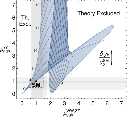
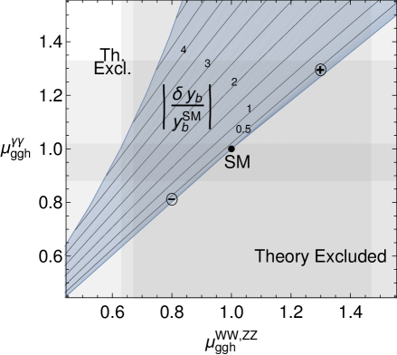
Figure 2: Contours of the bottom quark Yukawa correction $\displaystyle\left|\frac{\delta y_{b}}{y_{b}^{SM}}\right|$ with respect to the gluon fusion signal strengths $\mu_{ggh}^{VV}$ and $\mu^{\gamma\gamma}_{ggh}$. The right panel zooms in on the region marked by a dashed box in the left panel. The horizontal and vertical gray bands represent the experimental bounds set by the LHC RUN 1 (darker) and the preliminary data from LHC RUN 2 (lighter). The “Theory Excluded” regions are points excluded by the Brane Higgs Limit constraint. Each contour is traced by varying the phase of $\delta y_{b}$ and we include two parameter space points as example limits, marked by a $\oplus$ and a $\ominus$, representing, respectively, an overall enhancement or suppression with respect to the SM predictions.

As we have seen earlier, the Brane Higgs Limit condition is quite predictive, and easily falsifiable in the near future from LHC Higgs data. The first important point is that within our minimal general setup, all signal strengths associated with the Higgs will deviate from the SM values only due to shifts in the top and bottom quark Yukawa couplings. This means that ratios of Higgs signal strengths involving electroweak production processes, and decays through the same channels “$ii$”, should be equal to one, i.e

$$\frac{\mu^{ii}_{VBF}}{\mu^{ii}_{Wh}}=\frac{\mu^{ii}_{VBF}}{\mu^{ii}_{Zh}}=1$$ (41)

Also signal strengths involving decays into $WW$ should be equal to signals with decays into $ZZ$, i.e.

$$\frac{\mu^{WW}_{ggh}}{\mu^{ZZ}_{ggh}}=\frac{\mu^{WW}_{tth}}{\mu^{ZZ}_{tth}}=\frac{\mu^{WW}_{Vh}}{\mu^{ZZ}_{Vh}}=\frac{\mu^{WW}_{VBF}}{\mu^{ZZ}_{VBF}}=1.$$ (42)

These are strong model dependent predictions, likely testable at the present RUN 2 at the LHC.

Now, more specific to our setup, and as seen from Eqs. (31)-(34), the corrections to all of the Higgs signal strengths depend only on four parameters, i.e. the absolute values of the relative top and bottom Yukawa coupling deviations $|\delta y_{t}|$ and $|\delta y_{b}|$, and their two phases. Moreover, only the $t{\bar{t}}h$ signal strengths depend on all four parameters. We thus start exploring the dominant Higgs production mechanism, the gluon fusion process, paying particular attention to the signal strengths $\mu^{\gamma\gamma}_{ggh}$ and $\mu^{WW,ZZ}_{ggh}$. These depend only on the deviation of the bottom quark coupling (magnitude and phase). It is therefore possible to study the relationship between these two signal strengths, for different values of $\delta y_{b}$. This is plotted in Fig. 2, where we show that only a specific region in the ($\mu^{\gamma\gamma}_{ggh},\mu^{WW,ZZ}_{ggh})$ plane is allowed, due to the Brane Higgs Limit constraint. The horizontal and vertical gray bands correspond to limits set by LHC RUN 1 and preliminary LHC RUN 2 data, as summarized in Table 1. In the right panel of that figure, we zoom in the square enclosed by dashed lines in the left panel to consider signal strengths close to the SM model value, and we can see that the region where $\mu^{\gamma\gamma}_{ggh}<\mu^{WW,ZZ}_{ggh}$ is not allowed, thus providing a very simple and strong prediction of the scenario. Corrections in the direction $\mu^{\gamma\gamma}_{ggh}>\mu^{WW,ZZ}_{ggh}$ are possible, but require increasingly large deviations in the bottom Yukawa coupling. For relatively small values of $\delta y_{b}$, one can still obtain important deviations in the signals if one moves along the $\mu^{\gamma\gamma}_{ggh}\simeq\mu^{WW,ZZ}_{ggh}$ diagonal line. For future use, we choose two points along that line, close to the boundaries set by the LHC constraints. We denote them with a $\oplus$ and $\ominus$, and they represent either an overall enhancement in the $ggh$ signal strengths, or an overall suppression, with respect to the SM predictions.

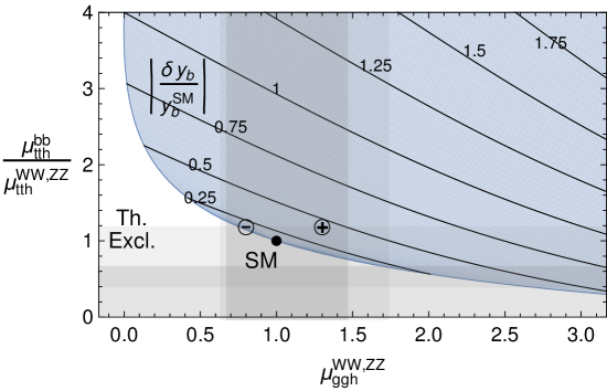
Figure 3: Contours of the bottom quark Yukawa correction $\displaystyle\left|\frac{\delta y_{b}}{y_{b}^{SM}}\right|$ with respect to the gluon fusion signal strength $\mu_{ggh}^{VV}$ and the ratio of the $t{\bar{t}}h$ signal strengths $\displaystyle\frac{\mu^{bb}_{tth}}{\mu_{tth}^{VV}}$. The horizontal and vertical grey bands represent the experimental bounds set by the LHC RUN 1 (darker) and the preliminary data from LHC RUN 2 (lighter). The “Th. Excl.” region comprises all points excluded by the Brane Higgs Limit constraint. Each contour is traced by varying the phase of $\delta y_{b}$ and we included two same parameter space points, marked by $\oplus$ and $\ominus$, as in the previous figure.

Once the gluon fusion signals have been fixed, we can study the effect on other signal strengths which receive corrections only through the bottom quark Yukawa coupling. In particular we can explore how the ratios $\displaystyle\frac{\mu^{bb}_{tth}}{\mu^{VV}_{tth}}=\frac{\mu^{bb}_{Vh}}{\mu^{VV}_{Vh}}$ behave as a function of $\mu^{VV}_{ggh}$ (all top quark Yukawa dependence cancels out in the ratio). This is shown in Fig. 3, where we consider variations of the ratio $\displaystyle\frac{\mu^{bb}_{tth}}{\mu^{VV}_{tth}}$ (with the corresponding LHC bounds represented by the horizontal gray bands), with respect to the gluon fusion strength $\mu^{bb}_{tth}$. As we can see, the current experimental data tend to prefer values for that ratio close to 1 or less, therefore putting some pressure on the allowed parameter space. We can see that if the $\mu^{bb}_{tth}$ signal strength is smaller than the $\mu^{VV}_{tth}$ one (both in $t{\bar{t}}h$ production), then the data prefers a slight enhancement in the gluon fusion production strength. Conversely, if the $\mu^{bb}_{tth}$ signal is enhanced, then gluon fusion signals should be suppressed. Overall, the deviations on the bottom quark Yukawa coupling must be kept small, unless the $\mu^{bb}_{tth}$ signal happens to be very much larger than the $\mu^{VV}_{tth}$ signal. The chosen example points $\oplus$ and $\ominus$ stay within a ratio of $\mu_{tth}$ production signals close to 1.

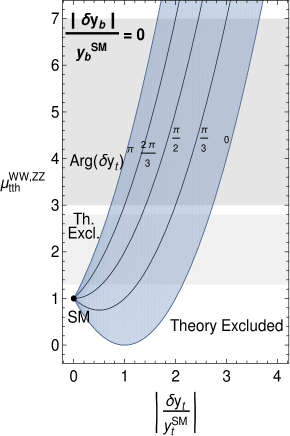
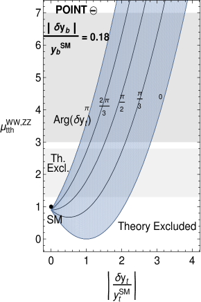
Figure 4: Higgs signal strength $\mu_{tth}^{VV}$ with respect to the top quark Yukawa coupling correction $\displaystyle\left|\frac{\delta y_{t}}{y_{t}^{SM}}\right|$. The contours trace points with constant value of the phase of $\delta y_{t}$, and the horizontal gray bands represent the experimental bounds set by the LHC RUN 1 (darker) and the preliminary data from LHC RUN 2 (lighter). The “Theory Excluded” regions are excluded by the Brane Higgs Limit constraint. In the left panel, we consider a parameter space point where the bottom Yukawa coupling is SM-like. In the central panel the bottom quark Yukawa coupling is corrected by 18% (point $\ominus$) and the right panel has a bottom quark Yukawa correction of 44% (point $\oplus$).

Once we analyzed the restriction on the deviations from bottom quark Yukawa couplings, we can investigate the signals that do depend on the top Yukawa coupling deviations. In Fig. 4 we choose to study the variation of $\mu^{VV}_{tth}$ with respect to the top Yukawa deviation $|\delta y_{t}|$. The rest of $t{\bar{t}}h$ signals strengths can be obtained from ratios of other Higgs production signals strengths, since for example $\displaystyle\mu^{\gamma\gamma}_{tth}=\frac{\mu^{\gamma\gamma}_{ggh}}{\mu^{VV}_{ggh}}\ \mu^{VV}_{tth}$. We fix the values of the bottom quark Yukawa coupling in three limits, i.e. when $y_{b}$ is SM-like ($\delta y_{b}=0$), when it has a 18% correction ($\left|\delta y_{b}/y_{b}^{SM}\right|=0.18$, corresponding to the point $\ominus$), and when it has a 44% correction ($\left|\delta y_{b}/y_{b}^{SM}\right|=0.44$, corresponding to the point $\oplus$). As can be seen in Fig. 4, for moderate values of $\delta y_{b}$ there is very mild dependence on $\delta y_{b}$, so that the three panels show very similar behavior of the signal strength as a function of the deviations in top quark Yukawa couplings. The parameter space region is a diagonal band, and we show contours of the phase of the top Yukawa shift $\delta y_{t}$, tracing the band diagonally. The dependence is very sensitive to variations in the phase of the shift of the top Yukawa coupling. We can clearly see that if the magnitude of the top Yukawa deviation is less than 1 (the natural expectation for heavy KK top partners), in order to obtain a signal enhancement (as hinted by LHC data), the phase must be close to $\pi$. This is in agreement with the perturbative expressions obtained earlier for the Yukawa shifts and it corresponds to values of the mass matrix phase $\theta^{t}_{2}$ close to 0.

III “Brane Higgs Limit” in Randall Sundrum models

In this section we describe briefly how to reproduce the previous phenomenological scenario within the context of the Randall Sundrum model RS1 . Consider a sector of a 5D scenario with a 5D top quark, i.e. a doublet fermion $Q(x,y)$ and a singlet $T(x,y)$ defined by the following action:

$$S=-i\int d^{4}xdy\sqrt{-g}\left[\bar{Q}D\!\!\!\!/Q+c_{q}\sigma^{\prime}\bar{Q}Q+\bar{T}D\!\!\!\!/T+c_{t}\sigma^{\prime}\bar{T}T\right.$$

$$\left.+\delta(y-y_{1})\left(\alpha_{qL}\bar{Q}_{L}\partial\!\!\!/Q_{L}+\alpha_{qR}\bar{Q}_{R}\partial\!\!\!/Q_{R}+\alpha_{tL}\bar{T}_{L}\partial\!\!\!/T_{L}+\alpha_{tR}\bar{T}_{R}\partial\!\!\!/T_{R}\right)\right.$$

$$\left.+\delta(y-y_{1})\left(Y_{1}H\bar{Q}_{L}T_{R}+Y_{2}H\bar{Q}_{R}T_{L}+h.c.\right)\right]$$ (43)

where $D\!\!\!\!/=\gamma_{A}e^{M}_{A}D_{M}$ and $\partial\!\!\!/=\gamma_{a}e^{\mu}_{a}\partial_{\mu}$, with $\gamma_{A}$ the 5D gamma matrices, $e^{M}_{A}$ the vielbein, and $D_{M}=(\partial_{M}+\Gamma_{M})$ the 5D covariant derivative involving the spin connection $\Gamma_{M}$, with $\Gamma_{\mu}=\frac{1}{2}\gamma_{5}\gamma_{\mu}\sigma^{\prime}$ and $\Gamma_{5}=0$. The fifth dimension is understood as an interval, with the boundary terms fixing the boundary conditions of the fields. We have added a set of fermion kinetic terms localized at the boundary $y=y_{1}$. Other boundary fermion kinetic terms, involving $y$-derivatives, are allowed but we leave them out for simplicity. Also note that we should only consider positive brane kinetic term coefficients $\alpha_{i}$, in order to avoid tachyons and/or ghosts delAguila:2006atw ; Carena:2004zn .

We also consider Higgs localized Yukawa couplings on the same boundary. Note that the doublet $Q$ is vector-like in 5D, and we define $Q=Q_{L}+Q_{R}$ and $T=T_{L}+T_{R}$ where $Q_{L},T_{L}$ and $Q_{R},T_{R}$ are the left and right handed components.

The background spacetime metric is assumed to take the form

$$ds^{2}=e^{-2\sigma(y)}\eta_{\mu\nu}dx^{\mu}dx^{\nu}+dy^{2}$$ (44)

where $\sigma(y)=ky$ is known as the warp factor (note that the signature is $(-,+,+,+,+)$) and with $k\sim M_{Pl}$ being the 5D curvature. We assume that $\sigma(y_{0})=1$ and $\sigma(y_{1})\simeq 34$ such that there are some 15 orders of magnitude of scale hierarchy between both boundaries.

In the absence of fermion brane kinetic terms (proportional to $\alpha_{i}$’s), this setup produces a tower of Kaluza Klein (KK) modes, such that the lowest lying modes of the doublet and singlet fields have wavefunctions exponentially localized towards either of the boundaries Davoudiasl:1999tf . The localization depends on the value of the 5D fermion mass parameters $c_{q}$ and $c_{t}$. When $c_{q}<1/2$ and $c_{t}>-1/2$, the zero modes of $Q$ and $T$ will be localized near the $y=y_{1}$ boundary, and will be identified as the two chiral components of the SM top quark. The rest of SM quarks will be obtained in a similar way, but the value of their bulk mass will localize them towards the $y=y_{0}$ boundary. Because the Higgs boson is by construction located at the $y=y_{1}$ boundary, the top quark will be “naturally” heavy (coupled strongly to the Higgs) whereas the rest of quarks quarks are lighter, since they couple to the Higgs weakly due to their geographical separation. On the other hand, the excited modes of all fermions will be very heavy and localized towards the $y=y_{1}$ boundary; their typical KK masses are of order $M_{\rm Pl}e^{-ky_{1}}\sim TeV$ and they will also couple strongly with the Higgs.

The scenario that we call the Brane Higgs Limit, requires the presence of $only$ the top quark and bottom quark heavy partners, which means the rest of KK partners should be decoupled (i.e. much heavier). For this we turn-on the fermion brane kinetic terms (the $\alpha_{i}$’s) of the 5D top and bottom quarks. There will still be massless fermion modes (associated to the SM top and bottom quarks), but it now becomes possible to lower the masses of the KK top and bottom modes. In general, it is possible to obtain analytically the associated KK spectrum (before electroweak symmetry breaking) in terms of Bessel functions. Nevertheless, since we are mainly interested in the top quark, it is much simpler and transparent to treat the special case where $c_{q}=c_{t}=0$. These simple bulk masses are perfectly top-like, and they have the advantage of producing very simple equations of motion. The usual dimensional reduction procedure involves a mixed separation of variables performed on the 5D fermions, i.e.

$$Q_{L}(x,y)=Q_{L}(y)t_{L}(x)$$ (45)

$$Q_{R}(x,y)=Q_{R}(y)t_{R}(x)$$ (46)

$$T_{L}(x,y)=T_{L}(y)t_{L}(x)$$ (47)

$$T_{R}(x,y)=T_{R}(y)t_{R}(x)$$ (48)

where $t_{L}(x)$ and $t_{R}(x)$ are the left and right handed components of 4D fermions (the lightest of which is the SM top quark). From there, one must solve for the KK profiles along the extra dimension $Q_{L}(y)$, $Q_{R}(y)$, $T_{L}(y)$ and $T_{R}(y)$. In the simple case of $c_{q}=c_{t}=0$, and before electroweak symmetry breaking,the equation for the profile $\tilde{Q}_{R}(y)=e^{-2\sigma(y)}Q_{R}(y)$, for example, becomes

$$\left(e^{-ky}\tilde{Q}^{\prime}_{R}\right)^{\prime}+m^{2}e^{ky}\tilde{Q}_{R}=0$$ (49)

with Dirichlet boundary condition on the $y=0$ boundary (since there are no kinetic terms there). The solution is simple,

$$\tilde{Q}_{R}(y)=N_{Q}\sin{\left(\frac{m(e^{ky}-1)}{k}\right)}$$ (50)

which obviously vanishes at $y=0$. The brane kinetic term on the $y=y_{1}$ boundary enforces a matching boundary condition at that location, and that boundary condition fixes the spectrum of the whole tower of KK modes. In this simple case, the KK spectrum of the 5D fermions $Q(x,y)$ and $T(x,y)$ is given by

$$\tan{\left(\frac{me^{ky_{1}}}{k}\right)}=-\sqrt{\frac{\alpha_{qL}}{\alpha_{qR}}}\tan{\left(me^{ky_{1}}\sqrt{\alpha_{qR}\alpha_{qL}}\right)}$$ (51)

and

$$\tan{\left(\frac{me^{ky_{1}}}{k}\right)}=-\sqrt{\frac{\alpha_{tL}}{\alpha_{tR}}}\tan{\left(me^{ky_{1}}\sqrt{\alpha_{tR}\alpha_{tL}}\right)},$$ (52)

in agreement with the flat metric limit considered in delAguila:2006atw . With a further simplification, taking $\alpha_{qR}=\alpha_{qL}=\alpha_{q}$ and $\alpha_{tR}=\alpha_{tL}=\alpha_{t}$, the conditions become

$$\tan{\left(\frac{me^{ky_{1}}}{k}\right)}=-\tan{\left(me^{ky_{1}}\alpha_{i}\right)}$$ (53)

with a spectrum given by

$$m_{n}=\frac{n\pi}{1+k\alpha_{i}}ke^{-ky_{1}}$$ (54)

for $n=0,1,2,3...$ This shows that, indeed, the spectrum of the KK tops can be significantly reduced in the presence of brane kinetic terms.

In the scenario we have in mind, only the 5D top and bottom quarks have large brane kinetic terms (without further justification) and therefore their associated KK modes can be much lighter than the rest, maybe as light as 1 TeV. At the same time, the rest of quarks and KK gauge bosons follow the usual RS pattern with KK masses maybe an order of magnitude larger ($\sim 10$ TeV). In this limit, flavor and precision electroweak bounds are much safer and the main phenomenological effects of the model may occur within the Higgs sector of the scenario.

If we decouple the $up$, $down$, $strange$ and $charm$ heavy KK quarks, the fermion mass matrices will involve only SM quarks along with KK $tops$ and KK $bottoms$. Mixing between light quarks localized near $y=0$ and heavier quarks localized near $y=y_{1}$ is going to be CKM suppressed, as usual in RS, and therefore the mass matrices to consider have the same form of those in Eqs. (2) and (3), but with the phases $\theta_{1}^{t}=\theta^{b}_{1}=0$. Indeed, the values of the off-diagonal terms in the mass matrices are now associated to the 5D Yukawa interactions localized at the $y=y_{1}$ brane and in this case are such that

$$Y_{t}^{0} = Y_{33}^{5D}f_{q_{L}}f_{t_{R}}$$ (55)

$$(Y_{1})_{nm} = Y_{33}^{5D}f_{Q^{n}_{L}}f_{T^{m}_{R}}$$ (56)

$$(Y_{qT})_{n} = Y_{33}^{5D}f_{q_{L}}f_{T^{n}_{R}}$$ (57)

$$(Y_{Qt})_{n} = Y_{33}^{5D}f_{Q^{n}_{L}}f_{t_{R}}$$ (58)

where $Y_{33}^{5D}$ is the 5D top Yukawa coupling, and where the $f_{i}$’s are the wavefunctions evaluated at the $y=y_{1}$ brane, with $q_{L}$ and $t_{R}$ being zero modes and $Q^{n}_{L}$ and $T^{n}_{R}$ representing the $n^{th}$ KK modes. We can see that all these terms share the same phase, so that we can set $\theta_{1}^{t}=\theta^{b}_{1}=0$.

Now, consider first a mass matrix with only one KK level ($n=1$), so that the matrices are exactly the same as before and thus the corresponding effect in Higgs production will come from the sum

$$\sum_{n}\left({\frac{y^{u}_{nn}}{m^{u}_{n}}}\right) = \frac{1}{v}\frac{1+3\varepsilon_{Q_{t}}\varepsilon_{T}\frac{|Y_{2}|}{|Y_{t}^{0}|}e^{i\theta^{t}_{2}}\left(1-\frac{|Y_{1}||Y_{t}^{0}|}{|Y_{Qt}||Y_{qT}|}\right)}{1+\varepsilon_{Q_{t}}\varepsilon_{T}\frac{|Y_{2}|}{|Y_{t}^{0}|}e^{i\theta^{t}_{2}}\left(1-\frac{|Y_{1}||Y_{t}^{0}|}{|Y_{Qt}||Y_{qT}|}\right)}.$$ (59)

It becomes then apparent that $\left(1-\frac{|Y_{1}||Y_{t}^{0}|}{|Y_{Qt}||Y_{qT}|}\right)=0$ due to the structure of the 5D couplings. It is important that the zero modes (SM top and bottom) come from the same 5D fermion as the KK modes, since the cancellation will only happen if they all share the same 5D Yukawa coupling. It turns out that it is simple to prove that if we take into account the complete towers of KK tops we still have

$$\sum^{\infty}_{n}\left({\frac{y^{u}_{nn}}{m^{u}_{n}}}\right) = \frac{1}{v}$$ (60)

and similarly for the bottom quarks, and thus the Higgs phenomenology of this scenario is indeed the same as in the Brane Higgs limit introduced earlier in a bottom-up approach, since relative corrections due to the KK modes of the up, down, strange and charm quarks, will scale as $\left(m_{KK}^{tops}/m_{KK}^{rest}\right)^{2}\sim 1\%$ (assuming that the rest of KK quarks are an order of magnitude heavier than KK tops/bottoms). Note that if the Higgs boson is not exactly localized at the boundary, then the cancellation will not be exact and new corrections will arise.

The contributions of this RS scenario to flavor and precision electroweak observables will be limited to effects due to the mixing of top and bottom with the vector-like partners, since we are considering very heavy KK gauge bosons ($\sim 10$ TeV). As pointed out earlier, Yukawa coupling mixing effects can lead to deviations in $|V_{tb}|$ which can easily be kept under control. Also effects can appear in the couplings $Z\to b_{R}{\bar{b}}_{R}$ and in $Z\to b_{L}{\bar{b}}_{L}$ Agashe:2006at , but since we consider the contribution from heavy KK gauge bosons to be suppressed, only Yukawa coupling mixings contribute, limiting the correction. In the usual RS scenario, it was already possible to find points in the $(c_{b},c_{q_{3}})$ plane, such that $Zb{\bar{b}}$ couplings remain within experimental bounds, with all the SM masses and mixings correctly obtained Casagrande:2008hr . In our scenario, finding parameter points safe from precision tests will be even easier, since the source of corrections is further limited.

IV Conclusion

In this work, we presented a simple explanation of the possible enhancement in the $t{\bar{t}}h$ associated production seen at the LHC. We added one $SU(2)$ doublet, and two $SU(2)$ singlet vector-like quarks to the matter content of the SM, as partners of the third family, and allow significant mixing between these with the third family only. After electroweak symmetry breaking, Yukawa couplings induce off-diagonal terms into the fermion mass matrix and, once in the physical basis, the top and bottom Yukawa couplings and their corresponding masses loose their SM alignment. With the proper sign (or phase), this misalignment can induce an enhancement of the top quark Yukawa coupling, and thus increase the cross section for $t{\bar{t}}h$ production. But the mechanism should also affect other observables in the Higgs sector, in particular, the cross section for Higgs production through gluon fusion. This is the main production channel for the SM Higgs and, being a radiative effect, it receives a contribution from all the fermions in the model. Each contribution is proportional to the ratio of the Yukawa fermion couplings to the fermion mass, so that the main contributions come from the top quark (with an enhanced Yukawa coupling), and from the new vector-like quarks.

We showed that working in a particular limit of parameter space, the corrections to gluon fusion caused by the top Yukawa coupling enhancement are exactly offset by the contributions of the new top partners, so that the overall top sector of our scenario (top quark plus heavy partners) gives the same contribution as the single top quark contribution in the SM. We call this scenario the Brane Higgs limit and it yields extremely predictive relationships between the productions cross sections ($gg$ and $t{\bar{t}}h$) and decay branching ratios for the Higgs bosons (into $WW,\,ZZ,\,b{\bar{b}}$ and $\gamma\gamma$), where the only free parameters are the absolute values of the shifts in the Yukawa couplings of the top and the bottom quarks, and their phases. For instance, in $t{\bar{t}}h$ production, if the branching ratio into $b{\bar{b}}$ is smaller than that into $VV$, then the gluon fusion production cross section must be also greater than its SM value, and conversely, an enhancement of the $b{\bar{b}}$ branching ratio in $t{\bar{t}}h$ production indicates a suppressed gluon fusion signal. Overall, the deviations in the Yukawa coupling of the bottom quark are constrained to be small, unless new data indicates a significant enhancement of the $b{\bar{b}}$ branching ratio. The scenario we consider predicts that any enhancement or suppression in the $\gamma\gamma$ signal should be matched with identical enhancement or suppression in $VV=WW,ZZ$ decays (for gluon fusion production), or at least remain always slightly higher than decays into $VV=WW,ZZ$, but never lower. Finally, a shift in the top quark Yukawa coupling will affect all $t{\bar{t}}h$ signals through the production cross section, and enhancement or suppression will depend on the phase of the shift.

The mixing in the top quark and bottom quark sectors should have also consequences in the Cabibbo-Kobayashi-Makskawa (CKM) mixing matrix $V_{CKM}$, as well as in precise electroweak measurements. We briefly discussed how the scenario affects (and thus is constrained by) the $V_{tb}$ entry of $V_{CKM}$ and the decay $Z\to b{\bar{b}}~{}(A_{FB}^{b})$.

Finally we showed that the phenomenology we described here depends on a specific structure of the fermion mixing matrix, mixing top quark with its partners. In particular the Yukawa coupling matrix should have a vanishing determinant, and thus some mechanism or flavor symmetry should be invoked to realize the scenario. The required structure is naturally realized in a Randall Sundrum model without a need for flavor symmetries. A key ingredient of this scenario is the presence of brane kinetic terms for the top and bottom, which can then result in lighter $n=1$ KK modes for the top and bottom partners, but heavy masses for all other KK modes. If the Higgs is localized exactly at the boundary, the overall phenomenology of the simple model introduced here is essentially recovered (i.e the cancellation of the terms happening in the gluon fusion calculation occurs by construction, even if in this case the effect comes from a complete tower of KK states).

The model presented here thus has a simple theoretical realization, is highly predictable, and can be tested (or ruled out) by more precise measurements of the Higgs signal strength in RUN 2 at LHC.

V Acknowledgments

M.T. would like to thank FRQNT for partial financial support under grant number PRCC-191578 and M.F. acknowledges NSERC support under grant number SAP105354.

References

- (1) V. Khachatryan et al. [CMS Collaboration], JHEP 1409, 087 (2014) Erratum: [JHEP 1410, 106 (2014)] doi:10.1007/JHEP09(2014)087, 10.1007/JHEP10(2014)106 [arXiv:1408.1682 [hep-ex]].
- (2) G. Aad et al. [ATLAS Collaboration], Phys. Lett. B 749, 519 (2015) doi:10.1016/j.physletb.2015.07.079 [arXiv:1506.05988 [hep-ex]].
- (3) CMS Collaboration [CMS Collaboration], CMS-PAS-HIG-16-022.
- (4) The ATLAS collaboration [ATLAS Collaboration], ATLAS-CONF-2016-58; The ATLAS collaboration [ATLAS Collaboration], ATLAS-CONF-2016-080.
- (5) CMS Collaboration [CMS Collaboration], CMS-PAS-HIG-17-004.
- (6) CMS Collaboration [CMS Collaboration], CMS-PAS-HIG-17-003.
- (7) G. Aad et al. [ATLAS and CMS Collaborations], JHEP 1608, 045 (2016) doi:10.1007/JHEP08(2016)045 [arXiv:1606.02266 [hep-ex]].
- (8) The ATLAS collaboration [ATLAS Collaboration], ATLAS-CONF-2016-081.
- (9) CMS Collaboration [CMS Collaboration], CMS-PAS-HIG-16-020.
- (10) CMS Collaboration [CMS Collaboration], CMS-PAS-HIG-16-033.
- (11) The ATLAS collaboration [ATLAS Collaboration], ATLAS-CONF-2016-068.
- (12) A. Angelescu, A. Djouadi and G. Moreau, Eur. Phys. J. C 76, no. 2, 99 (2016) doi:10.1140/epjc/s10052-016-3950-y [arXiv:1510.07527 [hep-ph]].
- (13) D. Choudhury, T. M. P. Tait and C. E. M. Wagner, Phys. Rev. D 65, 053002 (2002) doi:10.1103/PhysRevD.65.053002 [hep-ph/0109097]. D. E. Morrissey and C. E. M. Wagner, Phys. Rev. D 69, 053001 (2004) doi:10.1103/PhysRevD.69.053001 [hep-ph/0308001]; K. Kumar, W. Shepherd, T. M. P. Tait and R. Vega-Morales, JHEP 1008, 052 (2010) doi:10.1007/JHEP08(2010)052 [arXiv:1004.4895 [hep-ph]];
- (14) A. Azatov, O. Bondu, A. Falkowski, M. Felcini, S. Gascon-Shotkin, D. K. Ghosh, G. Moreau, A.Y. Rodriguez-Marrero and S. Sekmen, Phys. Rev. D 85, 115022 (2012) doi:10.1103/PhysRevD.85.115022 [arXiv:1204.0455 [hep-ph]]; B. Batell, D. McKeen and M. Pospelov, JHEP 1210, 104 (2012) doi:10.1007/JHEP10(2012)104 [arXiv:1207.6252 [hep-ph]]; D. McKeen, M. Pospelov and A. Ritz, Phys. Rev. D 86, 113004 (2012) doi:10.1103/PhysRevD.86.113004 [arXiv:1208.4597 [hep-ph]]; M. B. Voloshin, Phys. Rev. D 86, 093016 (2012) doi:10.1103/PhysRevD.86.093016 [arXiv:1208.4303 [hep-ph]]; B. Batell, S. Gori and L. T. Wang, JHEP 1301, 139 (2013) doi:10.1007/JHEP01(2013)139 [arXiv:1209.6382 [hep-ph]]; S. Dawson, E. Furlan and I. Lewis, Phys. Rev. D 87, no. 1, 014007 (2013) doi:10.1103/PhysRevD.87.014007 [arXiv:1210.6663 [hep-ph]]; J. A. Aguilar-Saavedra, R. Benbrik, S. Heinemeyer and M. Perez-Victoria, Phys. Rev. D 88, no. 9, 094010 (2013) doi:10.1103/PhysRevD.88.094010 [arXiv:1306.0572 [hep-ph]]; S. Gori, J. Gu and L. T. Wang, JHEP 1604, 062 (2016) doi:10.1007/JHEP04(2016)062 [arXiv:1508.07010 [hep-ph]]; C. H. Chen and T. Nomura, Phys. Rev. D 94, no. 3, 035001 (2016) doi:10.1103/PhysRevD.94.035001 [arXiv:1603.05837 [hep-ph]].
- (15) G. Aad et al. [ATLAS Collaboration], Phys. Rev. D 91, no. 11, 112011 (2015) doi:10.1103/PhysRevD.91.112011 [arXiv:1503.05425 [hep-ex]]. G. Aad et al. [ATLAS Collaboration], JHEP 1508, 105 (2015) doi:10.1007/JHEP08(2015)105 [arXiv:1505.04306 [hep-ex]]. G. Aad et al. [ATLAS Collaboration], Phys. Rev. D 92, no. 11, 112007 (2015) doi:10.1103/PhysRevD.92.112007 [arXiv:1509.04261 [hep-ex]].
- (16) P. Huang, A. Ismail, I. Low and C. E. M. Wagner, Phys. Rev. D 92, no. 7, 075035 (2015) doi:10.1103/PhysRevD.92.075035 [arXiv:1507.01601 [hep-ph]]; M. Badziak and C. E. M. Wagner, JHEP 1605 (2016) 123 doi:10.1007/JHEP05(2016)123 [arXiv:1602.06198 [hep-ph]]; M. Badziak and C. E. M. Wagner, JHEP 1702 (2017) 050 doi:10.1007/JHEP02(2017)050 [arXiv:1611.02353 [hep-ph]].
- (17) A. Das, N. Maru and N. Okada, arXiv:1704.01353 [hep-ph].
- (18) M. Frank, N. Pourtolami and M. Toharia, Phys. Rev. D 95, no. 3, 036007 (2017) doi:10.1103/PhysRevD.95.036007 [arXiv:1607.04534 [hep-ph]].
- (19) A. Azatov, M. Toharia and L. Zhu, Phys. Rev. D 80, 035016 (2009) doi:10.1103/PhysRevD.80.035016 [arXiv:0906.1990 [hep-ph]].
- (20) J. F. Gunion, H. E. Haber, G. L. Kane and S. Dawson, Front. Phys. 80, 1 (2000).
- (21) C. Patrignani et al. [Particle Data Group], Chin. Phys. C 40, no. 10, 100001 (2016). doi:10.1088/1674-1137/40/10/100001
- (22) C. Bobeth, A. J. Buras, A. Celis and M. Jung, JHEP 1704, 079 (2017); K. Ishiwata, Z. Ligeti and M. B. Wise, JHEP 1510, 027 (2015); G. Cacciapaglia, A. Deandrea, L. Panizzi, N. Gaur, D. Harada and Y. Okada, JHEP 1203, 070 (2012); A. K. Alok, S. Banerjee, D. Kumar, S. U. Sankar and D. London, Phys. Rev. D 92, 013002 (2015); S. A. R. Ellis, R. M. Godbole, S. Gopalakrishna and J. D. Wells, JHEP 1409, 130 (2014); G. Isidori, Y. Nir and G. Perez, Ann. Rev. Nucl. Part. Sci. 60, 355 (2010); G. Cacciapaglia, A. Deandrea, D. Harada and Y. Okada, JHEP 1011, 159 (2010); F. del Aguila, M. Perez-Victoria and J. Santiago, JHEP 0009, 011 (2000); G. Barenboim, F. J. Botella and O. Vives, Nucl. Phys. B 613, 285 (2001).
- (23) L. Randall and R. Sundrum, Phys. Rev. Lett. 83, 3370 (1999); ibid., Phys. Rev. Lett. 83, 4690 (1999).
- (24) F. del Aguila, M. Perez-Victoria and J. Santiago, JHEP 0302, 051 (2003) doi:10.1088/1126-6708/2003/02/051 [hep-th/0302023]; F. del Aguila, M. Perez-Victoria and J. Santiago, JHEP 0610, 056 (2006) doi:10.1088/1126-6708/2006/10/056 [hep-ph/0601222].
- (25) M. Carena, A. Delgado, E. Ponton, T. M. P. Tait and C. E. M. Wagner, Phys. Rev. D 71, 015010 (2005) doi:10.1103/PhysRevD.71.015010 [hep-ph/0410344].
- (26) H. Davoudiasl, J. L. Hewett and T. G. Rizzo, Phys. Lett. B 473, 43 (2000); S. Chang, J. Hisano, H. Nakano, N. Okada and M. Yamaguchi, Phys. Rev. D 62, 084025 (2000); T. Gherghetta and A. Pomarol, Nucl. Phys. B 586, 141 (2000). A. Pomarol, Phys. Lett. B 486, 153 (2000).
- (27) K. Agashe, A. Delgado, M. J. May and R. Sundrum, JHEP 0308, 050 (2003); K. Agashe, R. Contino, L. Da Rold and A. Pomarol, Phys. Lett. B 641, 62 (2006).
- (28) S. Casagrande, F. Goertz, U. Haisch, M. Neubert and T. Pfoh, JHEP 0810, 094 (2008).