Sharp rates of convergence for accumulated spectrograms

Abstract.

We investigate an inverse problem in time-frequency localization: the approximation of the symbol of a time-frequency localization operator from partial spectral information by the method of accumulated spectrograms (the sum of the spectrograms corresponding to large eigenvalues). We derive a sharp bound for the rate of convergence of the accumulated spectrogram, improving on recent results.

1. Introduction

In this article we obtain sharp rates of convergence for the approximation of the symbol of a time-frequency filter from (phaseless) measurements of its eigenspectrograms, using the method of accumulated spectrograms. The method is within the realm of inverse problems of time-frequency localization, where one aims to recover a localization operator from partial spectral information.

1.1. Time-frequency localization

In several branches of signal processing, signals change their frequency properties over time. It is the case of acoustical signals, such as music, where frequency variation is perceived as melody. Since the signal’s Fourier transform provides frequency information without localization in time, it is often preferable to represent a signal simultaneously in the time and frequency domain. The short-time Fourier transform of a function $f:{\mathbb{R}^{d}}\rightarrow{\mathbb{C}}$ is defined with the aid of a window function $g:{\mathbb{R}^{d}}\rightarrow{\mathbb{C}}$ as follows:

$$V_{g}f(z)=\int_{\mathbb{R}^{d}}f(t)\overline{g(t-x)}e^{-2\pi i\xi t}dt,\qquad z=(x,\xi)\in{\mathbb{R}^{2d}}\text{.}$$

The spectrogram of $f$, defined as

$$\mathrm{Spec}(f)(x,\xi):=\left|V_{g}f(x,\xi)\right|^{2}\text{,}$$

measures the intensity of the contribution to $f$ of the frequency $\xi$ near $x$. Time concentration for $f$ corresponds to decay of $\mathrm{Spec}(f)(x,\xi)$ in $x$, frequency concentration for $f$ corresponds to decay of $\mathrm{Spec}(f)(x,\xi)$ in $\xi$, and simultaneous concentration in time and frequency corresponds to decay of $\mathrm{Spec}(f)(x,\xi)$ in $(x,\xi)$.

Since a signal can only be observed and processed when concentrated within a bounded region of the time-frequency plane, a common practice in signal processing is to use a time-frequency filter that selects the portion of the spectrogram of a signal that is mostly concentrated on a given domain.

1.2. Localization operators

As a mathematical model of a time-frequency filter, Daubechies suggested an analogy to the Landau-Pollack-Slepian theory of prolate spheroidal functions [28, 29, 42, 27, 41]. This led to the following notion of localization operator ${H_{\Omega}}$ acting on a signal $f$. Given a compact set $\Omega\subseteq{\mathbb{R}^{2d}}$ and a function $f:{\mathbb{R}^{d}}\rightarrow{\mathbb{C}}$, let

(1.1) $${H_{\Omega}}f(t)=\int_{{\mathbb{R}^{2d}}}1_{\Omega}(x,\xi)V_{g}f(x,\xi)g(t-x)e^{2\pi i\xi t}dxd\xi\text{,}\qquad t\in{\mathbb{R}^{d}}\text{.}$$

The indicator function $1_{\Omega}(x,\xi)$ is called the symbol of ${H_{\Omega}}$. The spectrogram of ${H_{\Omega}}f$ is an approximation of $1_{\Omega}\cdot\mathrm{Spec}(f)$ - while $1_{\Omega}\cdot\mathrm{Spec}(f)$ does not in general correspond to the spectrogram of any signal.

More generally, it is usual to consider time-frequency localization operators associated with a general symbol $m\in L^{\infty}({\mathbb{R}^{2d}})$

(1.2) $${H_{m}}f(t)=\int_{{\mathbb{R}^{2d}}}m(x,\xi)V_{g}f(x,\xi)g(t-x)e^{2\pi i\xi t}dxd\xi\text{,}\qquad t\in{\mathbb{R}^{d}}\text{.}$$

These operators have been studied from the perspective of pseudodifferential calculus [23, 24, 10, 44].

If $\Omega\subseteq{\mathbb{R}^{2d}}$ is compact, then ${H_{\Omega}}$ is a compact and positive operator on $L^{2}(\mathbb{R}^{d})$ [9, 10, 16, 39]. Hence ${H_{\Omega}}$ can be diagonalized as

$${H_{\Omega}}f=\sum_{k\geq 1}{\lambda_{k}^{\Omega}}\left\langle f,h_{k}^{\Omega}\right\rangle h_{k}^{\Omega},\qquad f\in{L^{2}({\mathbb{R}^{d}})}\text{,}$$

where $\left\{{\lambda_{k}^{\Omega}}:k\geq 1\right\}$ are the non-zero eigenvalues of ${H_{\Omega}}$ ordered non-increasingly and $\left\{h_{k}^{\Omega}:k\geq 1\right\}$ are the corresponding orthonormal eigenfunctions. The quality of ${H_{\Omega}}$ as a simultaneous cut-off in the time-frequency variables can be described by its spectral properties, because the ($L^{2}$-normalized) eigenfunctions of $\left\{h_{k}^{\Omega}:k\geq 1\right\}$ of ${H_{\Omega}}$ maximize the time-frequency concentration of the spectrogram within $\Omega$. Indeed, since

$$\left\langle H_{\Omega}f,f\right\rangle=\int_{\Omega}\left|V_{g}f(x,\xi)\right|^{2}dxd\xi\text{,}$$

the min-max lemma for self-adjoint operators gives:

(1.3) $$\lambda_{k}^{\Omega}=\max\left\{\int_{\Omega}\left|V_{g}f(x,\xi)\right|^{2}dxd\xi:\left\|f\right\|=1,f\perp h_{1}^{\Omega},...,h_{k-1}^{\Omega}\right\}\text{.}$$

Thus, the eigenfunctions $h^{\Omega}_{k}$ have short-time Fourier transforms that are optimally concentrated on the target domain $\Omega$ in the $L^{2}$ sense. Time-frequency concentration can also be considered with respect to other metrics, and the fundamental results are contained in various uncertainty principles - see e.g. [30, 37, 38, 31, 22].

1.3. Inverse problems in time-frequency localization

The spectral problem of time-frequency localization presented in the previous section consists in describing the eigenfunctions and eigenvalues of ${H_{\Omega}}$. The corresponding inverse problem consist in recovering the different ingredients of ${H_{\Omega}}$ (the window $g$ or the domain $\Omega$) from (partial) spectral information. Thus, the inverse TF localization problem is a special case of the more general problem of channel identification [26, 8, 32, 33].

When $g$ is a Gaussian window and $\Omega$ is a disk, the eigenfunctions of ${H_{\Omega}}$ are Hermite functions, and the corresponding eigenvalues have an explicit expression (see Section 2 for more details). For the corresponding inverse problem, the following was established in [1].

Theorem 1.1 ([1]).

Let $g(t):=2^{1/4}e^{-\pi t^{2}}$, $t\in{\mathbb{R}}$, be the one-dimensional Gaussian and let $\Omega\subseteq{\mathbb{R}}^{2}$ be compact and simply connected. If one of the eigenfunctions of ${H_{\Omega}}$ is a Hermite function, then $\Omega$ is a disk centered at $0$.

Hence, for a Gaussian window $g$, the localization domain $\Omega$ is completely determined by the information that $\Omega\subseteq{\mathbb{R}^{2d}}$ is a simply connected set with given measure $|\Omega|$ and that one of the eigenfunctions of ${H_{\Omega}}$ is a Hermite function. However, the stylized assumptions of the Theorem 1.1 restrict its use in real applications. First, the restriction on the window $g$ is significant: the result holds only for Gaussian windows. It is not clear at all how to adapt the proofs in [1] to more general situations, since they depend on one variable complex analysis methods, which only apply to Gaussian windows [4]. In addition, Theorem 1.1 does not offer numerical stability: from the information that the eigenmodes of a time-frequency localization operator ${H_{\Omega}}$ look approximately like Hermite functions, one cannot conclude that the localization domain $\Omega$ is approximately a disk.

A more feasible approach to the approximate recovery of the localization domain from partial spectral information has been developed in [2], based on the concept of accumulated spectrogram. It provides a method for approximating the symbol of a localization operator from the intensities of the time-frequency representations of its eigenfunctions. Here, the chosen window $g$ plays only a minor role.

1.4. Symbol retrieval and the accumulated spectrogram

Suppose we can measure the spectrograms of the first eigenfunctions $h_{1}^{\Omega},\ldots,h_{N}^{\Omega}$ of the eigenvalue problem associated with ${H_{\Omega}}$ (that is, the eigenfunctions with higher time-frequency energy within the domain $\Omega$ - cf. (1.3)). The following is the central notion of the article.

Definition 1.2.

Let $A_{\Omega}$ be the smallest integer greater than or equal to $\left|\Omega\right|$. The accumulated spectrogram associated with $g$ and $\Omega$ is:

(1.4) $$\rho_{g,\Omega}(z):=\sum_{k=1}^{A_{\Omega}}\mathrm{Spec}_{g}\left(h_{k}^{\Omega}\right)(z)=\sum_{k=1}^{A_{\Omega}}\left|V_{g}h_{k}^{\Omega}(z)\right|^{2},\qquad z\in{\mathbb{R}^{2d}}\text{.}$$

(When the underlying window $g$ is clear from the context, we write $\rho_{\Omega}$ instead of $\rho_{g,\Omega}$.)

The idea of adding several uncorrelated spectrograms is not new. It is a basic tool in spectral estimation [7], it has been applied to the analysis of brain signals [46] and it is also an important step in the recent high-resolution time-frequency algorithm ConceFT [14]. The accumulated spectrogram has also been investigated in non-Euclidean contexts [20] - see also [25]. Numerical experiments show that when $N$ is close to the critical value $\approx\left|\Omega\right|$, the sum of the $N$ spectrograms that are most concentrated on $\Omega$ almost exhaust the domain $\Omega$; i.e., the accumulated spectrogram looks approximately like $1_{\Omega}$. The following result from [2] provides a rigorous formulation of this observation.

Theorem 1.3.

[2, Theorem 1.3] Let $g\in L^{2}({\mathbb{R}^{d})}$, $\left\|g\right\|_{2}=1$, and let $\Omega\subset{\mathbb{R}^{2d}}$ be compact. Then, in $L^{1}({\mathbb{R}^{2d})}$,

(1.5) $$\lim_{R\rightarrow\infty}\rho_{R\cdot\Omega}(R\cdot)\rightarrow 1_{\Omega}\text{.}$$

This shows that a large domain - $R\Omega$, with $R\gg 1$ - can be approximated, by sensing the intensity of the corresponding eigenspectrograms, without additional knowledge of the window. However, such a conclusion is only asymptotic. In practice, one needs a quantitative approximation estimate. In other words, we want to measure the rate of convergence to the limit in (1.5). We assume that $g$ satisfies the following time-frequency concentration condition:

(1.6) $$\lVert g\rVert_{M^{\ast}}^{2}:=\int_{\mathbb{R}^{2d}}\left|z\right|\left|V_{g}g(z)\right|^{2}dz<+\infty,$$

and let ${M^{\ast}}({\mathbb{R}^{d}})$ denote the class of all $L^{2}({\mathbb{R}^{d}})$ functions satisfying (1.6). The following has been obtained in [2].

Theorem 1.4 ([2]).

Let $g\in{M^{\ast}}({\mathbb{R}^{d}})$ with $\left\|g\right\|_{2}=1$ and $\Omega\subset\mathbb{R}^{2d}$ a compact set with finite perimeter. Then

(1.7) $$\left\|\rho_{g,\Omega}-1_{\Omega}\right\|_{L^{1}({\mathbb{R}^{2d}})}\leq C_{g}\sqrt{\left|\partial{\Omega}\right|}\sqrt{{|\Omega|}}\text{,}$$

where $\left|\partial{\Omega}\right|$ is the perimeter of $\Omega$ and $C_{g}$ is a constant that only depends on $g$.

The main result of this article is the following improvement of (1.7).

Theorem 1.5.

Let $g\in{M^{\ast}}({\mathbb{R}^{d}})$ with $\left\|g\right\|_{2}=1$ and $\Omega\subset\mathbb{R}^{2d}$ a compact set with finite perimeter and $\left|\partial{\Omega}\right|\geq 1$. Then

$$\left\|\rho_{g,\Omega}-1_{\Omega}\right\|_{L^{1}({\mathbb{R}^{2d}})}\leq C_{g}\left|\partial{\Omega}\right|\text{.}$$

Similar $L^{1}$ bounds have applications in signal analysis, namely in multi-taper stabilization of power spectrum estimation [3]. Besides being technically related to the main results [3], we expect the present results to be instrumental in non-stationary multi-taper estimation [7].

1.5. Phaseless approximation of time-frequency filters

The accumulated spectrogram is defined in terms of the absolute value of the short-time Fourier transform of the most significant eigenfunctions $V_{g}h^{\Omega}_{1},\ldots,V_{g}h^{\Omega}_{A_{\Omega}}$, and is thus related to the phase retrieval problem - see e.g. [18, 19, 5, 6]. Indeed, for a Schwartz-class window $g$, time-frequency localization operators (with general symbols as in (1.2)) satisfy a trace-norm estimate

$$\lVert H_{m}\rVert_{S^{1}}\lesssim\lVert m\rVert_{L^{1}},$$

where $S^{1}$ denotes the trace norm - see e.g. [10, 44]. Therefore, the estimate in Theorem 1.5 implies the spectral error bound

$$\lVert H_{\rho_{\Omega}}-H_{\Omega}\rVert_{S^{1}}=\lVert H_{\rho_{\Omega}-1_{\Omega}}\rVert_{S^{1}}\lesssim\lVert\rho_{\Omega}-1_{\Omega}\rVert_{L^{1}}\lesssim\left|\partial\Omega\right|.$$

In this way, the absolute values of the short-time Fourier transforms of the eigenfunctions $\{h^{\Omega}_{k}:k\geq 1\}$ lead to a spectral approximation of the operator $H_{\Omega}$.

1.6. Sharpness of the estimates

We establish the sharpness of the estimate in Theorem 1.5 by testing it on the family of all Euclidean balls.

Theorem 1.6.

Let $g\in L^{2}({\mathbb{R}^{d}})$ have norm 1 and let $B_{R}\subset{\mathbb{R}^{2d}}$ be the ball of radius $R>0$ centered at the origin. Then there exist constants $C,C^{\prime}$ such that

(1.8) $$CR^{2d-1}\leq\left\|\rho_{g,{B_{R}}}-1_{{B_{R}}}\right\|_{L^{1}({\mathbb{R}^{2d}})}\leq C^{\prime}R^{2d-1},\qquad R>0.$$

To compare, the estimate given by (1.7) is of the order $R^{2d-1/2}$. See Figures 2.1 and 2.2 for an illustration of Theorem 1.6, and [2] for numerical examples with other domains. Results in the spirit of Theorem 1.5 are also available in the context of spaces of weighted analytic functions (see e.g. [45]) and the corresponding bounds match the ones in Theorem 1.5.

2. Example: Gaussian windows

Let us consider the spectral problem associated with an operator of the form (1.1), and symbol $1_{B_{R}}(z)$, the indication function of a disk $B_{R}\subseteq{\mathbb{R}}^{2}$. Let

(2.1) $${\mathsf{h_{0}}}(t):=2^{1/4}e^{-\pi t^{2}},\text{ \ \ }t\in{\mathbb{R}}$$

be the one-dimensional Gaussian, normalized in $L^{2}$. Daubechies (on the signal side [11]) and Seip (directly on the phase space [40]) calculated the eigenfunctions and eigenvalues of the time-frequency localization operator with window ${\mathsf{h_{0}}}$ and domain $\Omega=B_{R}$. For all $R>0$, the eigenfunctions of $H_{B_{R}}$ are the Hermite functions:

$${\mathsf{h_{k}}}(t)=\frac{2^{1/4}}{\sqrt{k!}}\left(\frac{-1}{2\sqrt{\pi}}\right)^{k}e^{\pi t^{2}}\frac{d^{k}}{dt^{k}}\left(e^{-2\pi t^{2}}\right),\qquad k\geq 0.$$

Writing $z:=x+i\xi\in{\mathbb{C}}$, the short-time Fourier transform of the Hermite functions with respect to $h_{0}$ is

$$V_{{\mathsf{h_{0}}}}{\mathsf{h_{k}}}(z)=e^{\pi ix\xi}\left(\frac{\pi^{k}}{k!}\right)^{1/2}\overline{z}^{k}e^{-\pi\left|z\right|^{2}/2},\qquad k\geq 0\text{.}$$

Hence the corresponding spectrograms are

$$\left|V_{{\mathsf{h_{0}}}}{\mathsf{h_{k}}}(z)\right|^{2}=\frac{\pi^{k}}{k!}\left|z\right|^{2k}e^{-\pi\left|z\right|^{2}},\qquad k\geq 0\text{.}$$

Now, we have $\left|\Omega\right|=\left|B_{R}\right|=\pi$ $R^{2}$. Consequently, in Definition 1.2, we can take $N=\lceil\pi$ $R^{2}\rceil$. The resulting accumulated spectrogram is

(2.2) $$\rho_{{\mathsf{h_{0}}},B_{R}}(z)=\sum_{k=0}^{\lceil\pi R^{2}\rceil-1}\frac{\pi^{k}}{k!}\left|z\right|^{2k}e^{-\pi\left|z\right|^{2}}\text{.}$$

Theorem 1.5 says that, as $R\longrightarrow+\infty$,

(2.3) $$\rho_{{\mathsf{h_{0}}},B_{R}}(Rz)=\sum_{k=0}^{\lceil\pi R^{2}\rceil-1}\frac{\pi^{k}}{k!}R^{2k}\left|z\right|^{2k}e^{-\pi\left|Rz\right|^{2}}\longrightarrow 1_{B_{1}}(z),\mbox{ in }L^{1}({\mathbb{C}},dz)\text{,}$$

and gives a convergence rate of $O(1/R)$. Thus one recovers the indicator function of the disk. Theorem 1.5 provides us with much more information: since the limit function $1_{\Omega}$ does not depend on the window $g$, if one replaces the Gaussian (2.1) by an arbitrary $g\in{M^{\ast}}({\mathbb{R}^{d}})$ with $\left\|g\right\|_{2}=1$, the limit (2.3) would give the same result, and moreover the convergence rate is still $O(1/R)$. This gives a method to evaluate limits of the type (2.3) in situations where one has no explicit formulas for $V_{g}h^{\Omega}_{k}(z)$ or when the formulas are too complex to be analyzed directly.

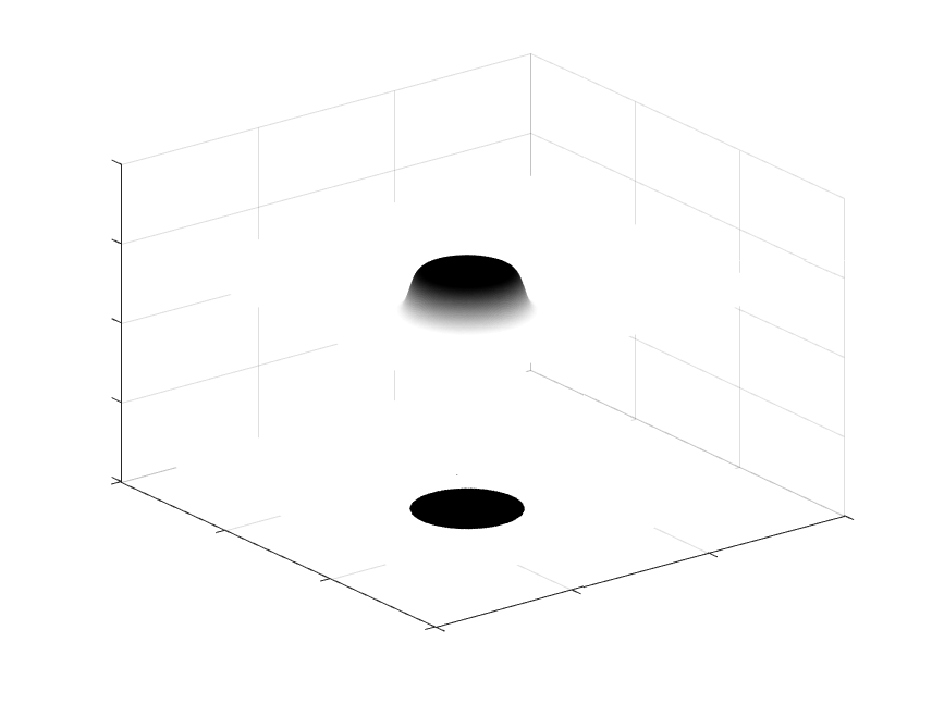
(a) The accumulated spectrogram corresponding to a circular domain of area $\approx$ 28.

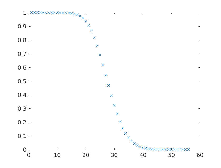
(b) A plot of the eigenvalues of the corresponding TF localization operator

Figure 2.1. An illustration of Theorem 1.6 with a Gaussian window.

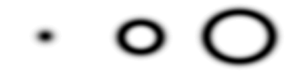
Figure 2.2. Some of the eigenspectrograms corresponding to Figure 2.1.

3. Some tools

3.1. Regularization by convolution

A function $f\in L^{1}(\mathbb{R}^{d})$ is said to have bounded variation if its distributional partial derivatives are finite Radon measures. We let $\mathit{BV}({\mathbb{R}^{d}})$ denote the space of functions of bounded variation. The variation of $f$ is defined as

$$\mathrm{Var}(f):=\sup\left\{\int_{{\mathbb{R}^{d}}}f(x)\mathrm{div}\phi(x)dx:\phi\in C_{c}^{1}(\mathbb{R}^{d},\mathbb{R}^{d}),\left|\phi(x)\right|_{2}\leq 1\right\}\text{,}$$

where $C_{c}^{1}(\mathbb{R}^{d},\mathbb{R}^{d})$ denotes the class of compactly supported $C^{1}$-vector fields and $\mathrm{div}$ is the divergence operator. If $f$ is continuously differentiable and has integrable derivatives, then $f\in\mathit{BV}({\mathbb{R}^{d}})$ and

$$\mathrm{Var}(f)=\int_{{\mathbb{R}^{d}}}\left|\nabla f(x)\right|_{2}dx\text{.}$$

A set $\Omega\subseteq{\mathbb{R}^{d}}$ is said to have finite perimeter if its indicator function $1_{\Omega}$ is of bounded variation. In this case, the corresponding perimeter is defined as

$$\left|\partial\Omega\right|=\mathrm{Var}(1_{\Omega})\text{.}$$

Every compact set $\Omega\subseteq{\mathbb{R}^{d}}$ with smooth boundary has a finite perimeter and its perimeter is the $(d-1)$-dimensional surface measure of its topological boundary (see [17, Chapter 5] for a detailed account of these topics). The following lemma quantifies the error introduced by convolution regularization. (For a proof, see [2, Lemma 3.2].)

Lemma 3.1.

Let $f\in\mathit{BV}({\mathbb{R}^{d}})$ and $\varphi\in{L^{1}({\mathbb{R}^{d}})}$ with $\int\varphi=1$. Then

$$\lVert f\ast\varphi-f\rVert_{L^{1}({\mathbb{R}^{d}})}\leq\mathrm{Var}(f)\int_{\mathbb{R}^{d}}\left|x\right|_{2}\left|\varphi(x)\right|dx\text{.}$$

In particular, for a set of finite perimeter $\Omega$:

$$\lVert 1_{\Omega}\ast\varphi-1_{\Omega}\rVert_{L^{1}({\mathbb{R}^{d}})}\leq\left|\partial{\Omega}\right|\int_{\mathbb{R}^{d}}\left|x\right|_{2}\left|\varphi(x)\right|dx\text{.}$$

3.2. Traces and disks

Proposition 3.2.

Let $g\in L^{2}({\mathbb{R}^{d}})$ have norm 1 and let $B_{R}\subset{\mathbb{R}^{2d}}$ be the ball of radius $R>0$ centered at the origin. Then there exist a constant $C>0$ such that

(3.1) $$\mathrm{trace}(H_{{B_{R}}})-\mathrm{trace}(H^{2}_{B_{R}})\geq CR^{2d-1}.$$

Proof.

This result is a special case of the asymptotics for the so-called plunge region of the eigenvalues of time-frequency localization operators [11, 13, 12] - that is, the region where the eigenvalues are away from both $0$ and $1$, cf. Figure 2.1; see also [35, 36, 23, 24, 15]. Concretely, (3.1) follows, for example, by combining Proposition 4.2 and Lemma 4.3 in [15]. (The result in [15] applies to certain families of domains that behave qualitatively like dilates of a single domain; the constant $C$ depends on the size of $\left|V_{g}g\right|$ near the origin.) ∎

4. Proof of Theorem 1.5

Step 1. A direct calculation shows that the traces of $H_{\Omega}$ and $H_{\Omega}^{2}$ are given by

(4.1) $$\mathrm{trace}(H_{\Omega})={|\Omega|},$$

(4.2) $$\mathrm{trace}(H_{\Omega}^{2})=\int_{\Omega}\int_{\Omega}\left|V_{g}g(z-z^{\prime})\right|^{2}dzdz^{\prime}\text{.}$$

(See for example [2, Lemma 2.1].). Therefore,

$$0\leq\mathrm{trace}(H_{\Omega})-\mathrm{trace}(H_{\Omega}^{2}) =\int_{\Omega}1-\left(1_{\Omega}\ast\left|V_{g}g\right|^{2}\right)(z)\,dz$$

$$\leq\lVert 1_{\Omega}\ast\left|V_{g}g\right|^{2}-1_{\Omega}\rVert_{L^{1}({\mathbb{R}^{2d}})}\text{.}$$

Hence, by Lemma 3.1 we conclude that

(4.3) $$0\leq\mathrm{trace}(H_{\Omega})-\mathrm{trace}(H_{\Omega}^{2})\leq\lVert g\rVert_{M^{\ast}}^{2}\left|\partial{\Omega}\right|\text{.}$$

Step 2. Since

$$\mathrm{trace}(H_{\Omega}) = \sum_{k\geq 1}{\lambda_{k}^{\Omega}},$$

$$\mathrm{trace}(H_{\Omega}^{2}) = \sum_{k\geq 1}{(\lambda_{k}^{\Omega}})^{2},$$

we have

$$\mathrm{trace}(H_{\Omega})-\mathrm{trace}(H_{\Omega}^{2})=\sum_{k\geq 1}{\lambda_{k}^{\Omega}}(1-{\lambda_{k}^{\Omega}})$$

$$\qquad=\sum_{k=1}^{A_{\Omega}}{\lambda_{k}^{\Omega}}(1-{\lambda_{k}^{\Omega}})+\sum_{k>A_{\Omega}}{\lambda_{k}^{\Omega}}(1-{\lambda_{k}^{\Omega}})$$

$$\qquad\geq\lambda_{A_{\Omega}}\sum_{k=1}^{A_{\Omega}}(1-{\lambda_{k}^{\Omega}})+(1-\lambda_{A_{\Omega}}^{\Omega})\sum_{k>A_{\Omega}}{\lambda_{k}^{\Omega}}$$

$$\qquad=\lambda_{A_{\Omega}}A_{\Omega}-\lambda_{A_{\Omega}}\sum_{k=1}^{A_{\Omega}}{\lambda_{k}^{\Omega}}+(1-\lambda_{A_{\Omega}}^{\Omega})\left(\left|\Omega\right|-\sum_{k=1}^{A_{\Omega}}{\lambda_{k}^{\Omega}}\right)$$

$$\qquad=\lambda_{A_{\Omega}}A_{\Omega}+\left|\Omega\right|(1-\lambda_{A_{\Omega}}^{\Omega})-\sum_{k=1}^{A_{\Omega}}{\lambda_{k}^{\Omega}}$$

$$\qquad=\left|\Omega\right|-\sum_{k=1}^{A_{\Omega}}{\lambda_{k}^{\Omega}}+\lambda_{A_{\Omega}}^{\Omega}(A_{\Omega}-\left|\Omega\right|)$$

$$\qquad\geq\left|\Omega\right|-\sum_{k=1}^{A_{\Omega}}{\lambda_{k}^{\Omega}}.$$

Therefore, using the estimate in (4.3), we obtain

(4.4) $$\left|\Omega\right|-\sum_{k=1}^{A_{\Omega}}{\lambda_{k}^{\Omega}}\leq C_{g}\left|\partial{\Omega}\right|\text{.}$$

Step 3. Since $0\leq\rho_{\Omega}(z)\leq 1$, we can estimate

(4.5) $$\int_{\Omega}\left|\rho_{\Omega}(z)-1_{\Omega}(z)\right|\,dz =\left|\Omega\right|-\int_{\Omega}\rho_{\Omega}(z)\,dz$$

$$=\left|\Omega\right|-\sum_{k=1}^{A_{\Omega}}\int_{\Omega}\left|V_{g}h^{\Omega}_{k}(z)\right|^{2}dz$$

$$=\left|\Omega\right|-\sum_{k=1}^{A_{\Omega}}\left<H_{\Omega}h^{\Omega}_{k},h^{\Omega}_{k}\right>$$

$$=\left|\Omega\right|-\sum_{k=1}^{A_{\Omega}}{\lambda_{k}^{\Omega}}.$$

Similarly,

(4.6) $$\int_{{\mathbb{R}^{2d}}\setminus\Omega}\left|\rho_{\Omega}(z)-1_{\Omega}(z)\right|\,dz =\int_{{\mathbb{R}^{2d}}\setminus\Omega}\rho_{\Omega}(z)\,dz=\sum_{k=1}^{A_{\Omega}}(1-{\lambda_{k}^{\Omega}})$$

(4.7) $$=A_{\Omega}-\sum_{k=1}^{A_{\Omega}}{\lambda_{k}^{\Omega}}$$

$$\leq 1+\left|\Omega\right|-\sum_{k=1}^{A_{\Omega}}{\lambda_{k}^{\Omega}}.$$

Using (4.4) and the fact that $\left|\partial{\Omega}\right|\geq 1$ we obtain the desired conclusion:

$$\int_{{\mathbb{R}^{d}}}\left|\rho_{\Omega}(z)-1_{\Omega}(z)\right|\,dz\leq 1+2\left(\left|\Omega\right|-\sum_{k=1}^{A_{\Omega}}{\lambda_{k}^{\Omega}}\right)\leq C_{g}\left|\partial{\Omega}\right|\text{.}$$

5. Proof of Theorem 1.6

In view of Theorem 1.5, we only need to prove the lower bound in (1.8). Let $\Omega\subseteq{\mathbb{R}^{2d}}$ be a compact domain with finite perimeter. Using (4.5), (4.6) and (4.7) we obtain

$$\int_{\mathbb{R}^{2d}}\left|\rho_{\Omega}(z)-1_{\Omega}(z)\right|\,dz =\left|\Omega\right|+A_{\Omega}-2\sum_{k=1}^{A_{\Omega}}{\lambda_{k}^{\Omega}}$$

$$=\left(A_{\Omega}-\sum_{k=1}^{A_{\Omega}}{\lambda_{k}^{\Omega}}\right)+\left(\mathrm{trace}(H_{\Omega})-\sum_{k=1}^{A_{\Omega}}{\lambda_{k}^{\Omega}}\right)$$

$$=\sum_{k=1}^{A_{\Omega}}(1-\lambda^{\Omega}_{k})+\sum_{k>A_{\Omega}}\lambda^{\Omega}_{k}$$

$$\geq\sum_{k=1}^{A_{\Omega}}\lambda^{\Omega}_{k}(1-\lambda^{\Omega}_{k})+\sum_{k>A_{\Omega}}\lambda^{\Omega}_{k}(1-\lambda^{\Omega}_{k})$$

$$=\mathrm{trace}(H_{\Omega})-\mathrm{trace}(H^{2}_{\Omega}).$$

We apply these calculations to $\Omega=B_{R}$ to obtain

(5.1) $$\int_{\mathbb{R}^{2d}}\left|\rho_{{B_{R}}}(z)-1_{{B_{R}}}(z)\right|\,dz\geq\mathrm{trace}(H_{{B_{R}}})-\mathrm{trace}(H^{2}_{{B_{R}}}).$$

Therefore, by Proposition 3.2,

(5.2) $$\int_{\mathbb{R}^{2d}}\left|\rho_{{B_{R}}}(z)-1_{{B_{R}}}(z)\right|\,dz\gtrsim R^{2d-1},$$

as desired.

6. Acknowledgements

Part of the research for this article was conducted while L. D. A. and J. L. R. visited the Program in Applied and Computational Mathematics at Princeton University. They thank PACM and in particular Prof. Amit Singer for their kind hospitality. The figures were prepared with the Large Time-Frequency Analysis Toolbox (LTFAT) [43, 34].

References

• [1] L. D. Abreu and M. Dörfler. An inverse problem for localization operators. Inverse Problems, 28(11):115001, 16, 2012.
• [2] L. D. Abreu, K. Gröchenig, and J. L. Romero. On accumulated spectrograms. Trans. Amer. Math. Soc., 368(5):3629 – 3649, 2016.
• [3] L. D. Abreu, and J. L. Romero. MSE estimates for multitaper spectral estimation and off-grid compressive sensing. Preprint. Arxiv: 1703.08190.
• [4] G. Ascensi and J. Bruna. Model space results for the Gabor and wavelet transforms. IEEE Trans. Inform. Theory, 55(5):2250–2259, 2009.
• [5] R. M. Balan, B. G. Bodmann, P. G. Casazza, and D. Edidin. Painless reconstruction from magnitudes of frame coefficients. J. Fourier Anal. Appl., 15 (2009), no. 4, 488-501.
• [6] A. S. Bandeira, J. Cahill, D. G. Mixon, A. A. Nelson. Saving phase: Injectivity and stability for phase retrieval. Appl. Comput. Harmon. Anal., 37 (2014), no. 1, 106-125.
• [7] M. Bayram, R. G. Baraniuk. Multiple window time-varying spectrum estimation. In Nonlinear and Nonstationary Signal Processing (Cambridge, 1998), 292-316. Cambridge Univ. Press, Cambridge, 2000.
• [8] P. A. Bello. Measurement of random time-variant linear channels. IEEE Trans. Inform. Theory, 15(4):469–475, 1969.
• [9] P. Boggiatto, E. Cordero, and K. Gröchenig. Generalized anti-Wick operators with symbols in distributional Sobolev spaces. Integr. Equ. Oper. Theory, 48(4):427–442, 2004.
• [10] E. Cordero and K. Gröchenig. Time-frequency analysis of localization operators. J. Funct. Anal., 205(1):107–131, 2003.
• [11] I. Daubechies. Time-frequency localization operators: a geometric phase space approach. IEEE Trans. Inform. Theory, 34(4):605–612, July 1988.
• [12] I. Daubechies. The wavelet transform, time-frequency localization and signal analysis. IEEE Trans. Inform. Theory, 36(5):961–1005, 1990.
• [13] I. Daubechies and T. Paul. Time-frequency localisation operators - a geometric phase space approach: II. The use of dilations. Inverse Problems, 4(3):661–680, 1988.
• [14] I. Daubechies, Y. Wang, and H. Wu. ConceFT: concentration of frequency and time via a multitapered synchrosqueezed transform. Philosophical Transactions of the Royal Society of London Series A, 374:20150193, apr 2016.
• [15] F. DeMari, H. G. Feichtinger, and K. Nowak. Uniform eigenvalue estimates for time-frequency localization operators. J. London Math. Soc., 65(3):720–732, 2002.
• [16] M. Dörfler and J. L. Romero. Frames adapted to a phase-space cover. Constr. Approx., 39(3):445–484, 2014.
• [17] L. C. Evans and R. F. Gariepy. Measure Theory and Fine Properties of Functions. Studies in Advanced Mathematics. CRC Press, Boca Raton, 1992.
• [18] Ph. Jaming. Phase Retrieval Techniques for Radar Ambiguity Problems. J. Fourier Anal. Appl. 5 (1999), 313-333.
• [19] Ph. Jaming and A. Powell. Uncertainty principles for orthonormal bases. J. Funct Anal. 243 (2007), 611-630.
• [20] S. Ghobber. Some results on wavelet scalograms. Int. J. Wavelets Multiresolut. Inf. Process., DOI: 10.1142/S0219691317500199.
• [21] K. Gröchenig. Foundations of Time-Frequency Analysis. Appl. Numer. Harmon. Anal. Birkhäuser Boston, Boston, MA, 2001.
• [22] K. Gröchenig and E. Malinnikova. Phase space localization of Riesz bases for ${L}^{2}({R}^{d})$. Rev. Mat. Iberoam. 29(1):115–134, 2013.
• [23] C. Heil, J. Ramanathan, and P. Topiwala. Asymptotic Singular Value Decay of Time-frequency Localization Operators, in ”Wavelet Applications in Signal and Image Processing II, Proc. SPIE”, Vol.2303 (1994) p.15–24.
• [24] C. Heil, J. Ramanathan, and P. Topiwala. Singular values of compact pseudodifferential operators. J. Funct. Anal., 150(2):426–452, 1997.
• [25] O. Hutník. Wavelets from Laguerre polynomials and Toeplitz-type operators. Integral Equations Operator Theory. 71 (2011), no. 3, 357-388.
• [26] T. Kailath. Measurements on time-variant communication channels. IEEE Trans. Inform. Theory, 8(5):229– 236, 1962.
• [27] H. J. Landau. Necessary density conditions for sampling an interpolation of certain entire functions. Acta Math., 117:37–52, 1967.
• [28] H. J. Landau and H. O. Pollak. Prolate spheroidal wave functions, Fourier analysis and uncertainty II. Bell System Tech. J., 40:65–84, 1961.
• [29] H. J. Landau and H. O. Pollak. Prolate spheroidal wave functions, Fourier analysis and uncertainty III: The dimension of the space of essentially time- and band-limited signals. Bell System Tech. J., 41:1295–1336, 1962.
• [30] E. H. Lieb. Integral bounds for radar ambiguity functions and Wigner distributions. J. Math. Phys., 31(3):594–599, 1990.
• [31] A. Olivero, B. Torrésani, R. Kronland-Martinet. Refined support and entropic uncertainty inequalities. IEEE Trans. Audio, Speech and Language Processing, 21:8 (2013), pp. 1550-1559.
• [32] G. E. Pfander. Measurement of time-varying multiple-input multiple-output channels. Appl. Comput. Harmon. Anal., 24(3):393–401, 2008.
• [33] G. E. Pfander and D. F. Walnut. Measurement of time-variant channels. IEEE Trans. Inform. Theory, 52(11):4808–4820, November 2006.
• [34] Z. Průša, P. L. Søndergaard, N. Holighaus, C. Wiesmeyr, and P. Balazs. The Large Time-Frequency Analysis Toolbox 2.0. In M. Aramaki, O. Derrien, R. Kronland-Martinet, and S. Ystad, editors, Sound, Music, and Motion, Lecture Notes in Computer Science, pages 419–442. Springer International Publishing, 2014.
• [35] J. Ramanathan and P. Topiwala. Time-frequency localization via the Weyl correspondence. SIAM J. Math. Anal., 24(5):1378–1393, 1993.
• [36] J. Ramanathan and P. Topiwala. Time-frequency localization and the spectrogram. Appl. Comput. Harmon. Anal., 1(2):209–215, 1994.
• [37] B. Ricaud and B. Torrésani. A survey of uncertainty principles and some signal processing applications. Adv. Comput. Math., 40:3 (2014), pp. 629-650.
• [38] B. Ricaud and B. Torrésani. Refined support and entropic uncertainty inequalities applications. IEEE Trans. Inform. Theory, 59:7 (2013), pp. 4272-4279.
• [39] J. L. Romero. Characterization of coorbit spaces with phase-space covers. J. Funct. Anal., 262(1):59–93, 2012.
• [40] K. Seip. Reproducing formulas and double orthogonality in Bargmann and Bergman spaces. SIAM J. Math. Anal., 22(3):856–876, 1991.
• [41] D. Slepian, Some comments on Fourier analysis, uncertainty and modeling, SIAM Rev. 25 (1983) 379-393.
• [42] D. Slepian and H. O. Pollak. Prolate Spheroidal Wave Functions, Fourier Analysis and Uncertainty I. I. Bell Syst. Tech.J., 40(1):43–63, 1961.
• [43] P. L. Søndergaard, B. Torrésani, and P. Balazs. The Linear Time Frequency Analysis Toolbox. International Journal of Wavelets, Multiresolution Analysis and Information Processing, 10(4), 2012.
• [44] N. Teofanov. Continuity and Schatten-von Neumann properties for localization operators on modulation spaces. Mediterr. J. Math. 13 (2016), no. 2, 745-758.
• [45] G. Tian. On a set of polarized Kähler metrics on algebraic manifolds. J. Differential Geom. 32 (1990), no. 1, 99-130.
• [46] J. Xiang, Q. Luo, R. Kotecha, A. Korman, F. Zhang, H. Luo, H. Fujiwara, N. Hemasilpin, D. F. Rose Accumulated source imaging of brain activity with both low and high-frequency neuromagnetic signals Front Neuroinform. 2014; 8: 57.