Transition from vibrational to rotational characters in low-lying states of hypernuclei

Abstract

In order to clarify the nature of hypernuclear low-lying states, we carry out a comprehensive study for the structure of ${}^{144-154}_{~{}~{}~{}~{}~{}~{}~{}~{}\Lambda}$Sm-hypernuclei, which exhibit a transition from vibrational to rotational characters as the neutron number increases. To this end, we employ a microscopic particle-core coupling scheme based on a covariant density functional theory. We find that the positive-parity ground-state band in the hypernuclei shares a similar structure to that of the corresponding core nucleus. That is, regardless of whether the core nucleus is spherical or deformed, each hypernuclear state is dominated by the single configuration of the $\Lambda$ particle in the $s_{1/2}$ state ($\Lambda s_{1/2}$) coupled to one core state of the ground band. In contrast, the low-lying negative-parity states mainly consist of $\Lambda p_{1/2}$ and $\Lambda p_{3/2}$ configurations coupled to plural nuclear core states. We show that, while the mixing amplitude between these configurations is negligibly small in spherical and weakly-deformed nuclei, it strongly increases as the core nucleus undergoes a transition to a well-deformed shape, being consistent with the Nilsson wave functions. We demonstrate that the structure of these negative-parity states with spin $I$ can be well understood based on the $LS$ coupling scheme, with the total orbital angular momentum of $L=[I\otimes 1]$ and the spin angular momentum of $S=1/2$.

I Introduction

With the advent of the high-resolution Ge detector array, “Hyperball”, the $\gamma$-ray spectroscopy has been carried out for many hypernuclei Hashimoto and Tamura (2006). We particularly mention the measurement for ${}^{13}_{~{}\Lambda}$C, which has provided a quantitative information on the spin-orbit splittings Ajimura et al. (2001). In this experiment, the energy difference between the $1/2^{-}$ and $3/2^{-}$ states was determined to be $152\pm 54\pm 36$ keV, which has been interpreted as the spin-orbit splitting between 1$p_{1/2}$ and 1$p_{3/2}$ hyperon states in ${}^{13}_{~{}\Lambda}$C. This measurement, together with other measurements, thus has provided a solid evidence for that the spin-orbit splitting of hyperon states is smaller than that of nucleons, by more than one order of magnitude Hashimoto and Tamura (2006), which had been explained theoretically in terms of several different mechanisms Brockmann and Weise (1977); Noble (1980); Boguta and Bohrmann (1981); Boussy (1981).

A similar interpretation in other hypernuclei may need a caution, however. That is, the previous studies Motoba et al. (1985); Mei et al. (2014, 2015, 2016) have demonstrated that most $\Lambda$ hypernuclei are different from the ${}^{13}_{~{}\Lambda}$C, in a sense that the lowest $1/2^{-}$ and $3/2^{-}$ states cannot be naively interpreted as pure 1$p_{1/2}$ and 1$p_{3/2}$ hyperon states, respectively, due to a large effect of configuration mixings. This perturbs an interpretation of their energy difference as the spin-orbit splitting for the $p$ orbits. It has been shown that the amplitudes of the configuration mixing depend much on the the collective properties of the core nuclei Motoba et al. (1983); Bandō et al. (1983); Hiyama et al. (2000).

In this paper, we investigate systematically the nature of configuration mixing in several hypernuclei which exhibit different collective properties. The Sm isotopes around $N\sim 90$ provide an ideal playground for this purpose, even though the production of these hypernuclei may still be difficult at this moment, since it is well known that they exhibit a shape phase transition from vibrational to rotational characters as the number of neutron increases Casten and Zamfir (2001). To this end, we shall use the microscopic particle-core coupling scheme, based on the covariant density functional theory. It is worth mentioning that a covariant density functional theory has been successfully applied to the shape phase transition in ordinary Sm nuclei  Meng et al. (2005); Nikšić et al. (2007); Li et al. (2009).

The paper is organized as follows. In Sec. II, we briefly introduce the microscopic particle-core scheme for hypernuclei, which uses results of the multi-reference covariant density functional theory for nuclear core excitations. In Sec. III, we apply this method to the low-lying states of the Sm isotopes as well as the Sm $\Lambda$ hypernuclei, and discuss the nature of low-lying collective states in these hypernuclei. We particularly discuss how the configuration mixing alters as the shape of a core nucleus changes from spherical to deformed. We then summarize the paper in Sec. IV.

II method

II.1 Multi-reference covariant density functional theory for nuclear core excitations

We describe low-lying states of hypernuclei in the particle-core coupling scheme. The first step in this method is to construct the low-lying states of the core nuclei. To this end, we adopt the multi-reference covariant density functional theory (MR-CDFT) Yao et al. (2010, 2014). In the MR-CDFT, the wave function of each nuclear core state is obtained as a superposition of a set of quantum-number projected mean-field reference states, $|\beta\rangle$. Here, the reference states $|\beta\rangle$ are obtained with deformation constrained relativistic mean-field plus BCS calculations with the quadrupole deformation parameter $\beta$. These states are then projected onto states with a good quantum number of angular momentum and particle number as,

$$|\Phi_{IM}(\beta)\rangle=\hat{P}^{I}_{MK}\hat{P}^{N}\hat{P}^{Z}|\beta\rangle,$$ (1)

where $\hat{P}^{I}_{MK}$ is the angular momentum projection operator, and $\hat{P}^{N}$ and $\hat{P}^{Z}$ are the particle number projection operators for neutron and proton, respectively. For simplicity, we impose axial symmetry on the reference mean-field states, and thus the $K$ quantum number in Eq. (1) is zero. Following the philosophy of the generator coordinate method (GCM), the wave functions in the MR-CDFT are then constructed by superposing the projected wave functions as,

$$|\Phi_{nIM}\rangle=\sum_{\beta}F_{nI}(\beta)|\Phi_{IM}(\beta)\rangle.$$ (2)

Here, the weight function $F_{nI}(\beta)$ and the energy for the state $|\Phi_{nI}\rangle$ are obtained by solving the Hill-Wheeler-Griffin (HWG) equation, which is derived from the variational principle Ring and Schuck (1980).

In this paper, we calculate the Hamiltonian kernel in the HWG equation with the mixed-density prescription. That is, we assume the same functional form for the off-diagonal elements of the energy overlap (sandwiched by two different reference states) as that for the diagonal elements, by replacing all the densities and currents with the mixed ones  Yao et al. (2009, 2010). In the calculations shown below, we adopt the PC-F1 parametrization Bürvenich et al. (2002) for the relativistic point-coupling energy functional.

II.2 Microscopic particle-core coupling scheme for $\Lambda$ hypernuclei

We next construct the hypernuclear wave functions by expanding them on the nuclear core states, Eq. (2), which provide a set of basis. The resultant wave functions read,

$$\Psi_{JM}(\mbox{\boldmath$r$},\{\mbox{\boldmath$r$}_{i}\})=\sum_{n,\ell,j,I}{\mathscr{R}}_{j\ell nI}(r)[{\mathscr{Y}}_{j\ell}(\hat{\mbox{\boldmath$r$}})\otimes\Phi_{nI}(\{\mbox{\boldmath$r$}_{i}\})]^{(JM)},$$ (3)

where $r$ and $\mbox{\boldmath$r$}_{i}$ are the coordinates of the $\Lambda$ hyperon and the nucleons, respectively. ${\mathscr{R}}_{j\ell nI}(r)$ and ${\mathscr{Y}}_{j\ell}(\hat{\mbox{\boldmath$r$}})$ are the radial wave function and the spin-angular wave function for the $\Lambda$-particle, respectively. The index $n=1,2,\ldots$ distinguishes different core states with the same angular momentum $I$. In our previous publications Mei et al. (2014, 2015, 2016), we have called this method “the microscopic particle-rotor model”, since we have mainly considered couplings of a $\Lambda$ particle to rotational states of deformed core nuclei. We instead call it “the microscopic particle-core coupling scheme” in this paper, as we deal with both spherical and deformed core nuclei.

The radial wave functions, ${\mathscr{R}}_{j\ell nI}(r)$, in Eq. (3) and the energy of the state, $E_{J}$, are obtained by solving the equation $\hat{H}|\Psi_{JM}\rangle=E_{J}|\Psi_{JM}\rangle$. We assume that the Hamiltonian $\hat{H}$ for the whole $\Lambda$ hypernucleus is given by Mei et al. (2016),

$$\hat{H}=\hat{T}_{\Lambda}+\hat{H}_{\rm c}+\sum^{A_{c}}_{i=1}\hat{V}^{N\Lambda}(\mbox{\boldmath$r$},\mbox{\boldmath$r$}_{i}),$$ (4)

where $\hat{T}_{\Lambda}$ is the relativistic kinetic energy for the $\Lambda$ particle and $\hat{H}_{c}$ is the many-body Hamiltonian for the core nucleus, satisfying $\hat{H}_{c}|\Phi_{nI}\rangle=E_{nI}|\Phi_{nI}\rangle$. The last term on the right side of Eq. (4) represents the interaction term between the $\Lambda$ particle and the nucleons in the core nucleus, where $A_{c}$ is the mass number of the core nucleus. We here use the $N\Lambda$ interaction derived from the point-coupling energy functional with the PCY-S4 parametrization Tanimura and Hagino (2012),

$$\hat{V}^{N\Lambda}_{\rm S}(\mbox{\boldmath$r$},\mbox{\boldmath$r$}_{i})= \alpha_{S}^{N\Lambda}\gamma^{0}_{\Lambda}\delta(\mbox{\boldmath$r$}-\mbox{\boldmath$r$}_{i})\gamma^{0}_{N}+\delta_{S}^{N\Lambda}\gamma^{0}_{\Lambda}\Big{[}\overleftarrow{\nabla}^{2}\delta(\mbox{\boldmath$r$}-\mbox{\boldmath$r$}_{i})$$

$$+ \delta(\mbox{\boldmath$r$}-\mbox{\boldmath$r$}_{i})\overrightarrow{\nabla}^{2}+2\overleftarrow{\nabla}\cdot\delta(\mbox{\boldmath$r$}-\mbox{\boldmath$r$}_{i})\overrightarrow{\nabla}\Big{]}\gamma^{0}_{N},$$ (5)

$$\hat{V}^{N\Lambda}_{\rm V}(\mbox{\boldmath$r$},\mbox{\boldmath$r$}_{i})= \alpha_{V}^{N\Lambda}\delta(\mbox{\boldmath$r$}-\mbox{\boldmath$r$}_{i})+\delta_{V}^{N\Lambda}\Big{[}\overleftarrow{\nabla}^{2}\delta(\mbox{\boldmath$r$}-\mbox{\boldmath$r$}_{i})$$

$$+ \delta(\mbox{\boldmath$r$}-\mbox{\boldmath$r$}_{i})\overrightarrow{\nabla}^{2}+2\overleftarrow{\nabla}\cdot\delta(\mbox{\boldmath$r$}-\mbox{\boldmath$r$}_{i})\overrightarrow{\nabla}\Big{]},$$ (6)

$$\hat{V}^{N\Lambda}_{\rm Ten}(\mbox{\boldmath$r$},\mbox{\boldmath$r$}_{i})= i\alpha_{T}^{N\Lambda}\gamma^{0}_{\Lambda}\Big{[}\overleftarrow{\nabla}\delta(\mbox{\boldmath$r$}-\mbox{\boldmath$r$}_{i})+\delta(\mbox{\boldmath$r$}-\mbox{\boldmath$r$}_{i})\overrightarrow{\nabla}\Big{]}\cdot\mbox{\boldmath$\alpha$}.$$ (7)

In practice, the equation $\hat{H}|\Psi_{JM}\rangle=E_{J}|\Psi_{JM}\rangle$ is transformed into coupled-channels equations in the relativistic framework, in which all the diagonal and off-diagonal potentials are determined from the MR-CDFT calculation. We solve the coupled-channels equations by expanding the four-component radial wave function ${\mathscr{R}}_{j\ell nI}(r)$ on a spherical harmonic oscillator basis. See Refs. Mei et al. (2014, 2015, 2016) for more details on the framework.

III Results and discussion

Let us now apply the microscopic particle-core coupling scheme to Sm hypernuclei and discuss their low-lying collective states. To this end, we generate the reference states $|\beta\rangle$ by expanding the single-particle wave functions on a harmonic oscillator basis with 12 major shells. In the particle-number and angular-momentum projection calculations, we choose the number of mesh points to be 9 for the gauge angle in $[0,\pi]$, and 16 for the Euler angle $\theta$ in the interval $[0,\pi]$. In the coupled-channels calculations, we include up to $l_{\rm max}=19$, $j_{\rm max}=37/2$, and $n_{\rm max}=3$ in the total wave function, Eq. (3). For each $j,l,n,$ and $I$, we include up to 18 (19) major shells in the expansion of the upper (lower) component of radial wave functions on the spherical harmonic oscillator basis.

III.1 Shape transition in Sm isotopes

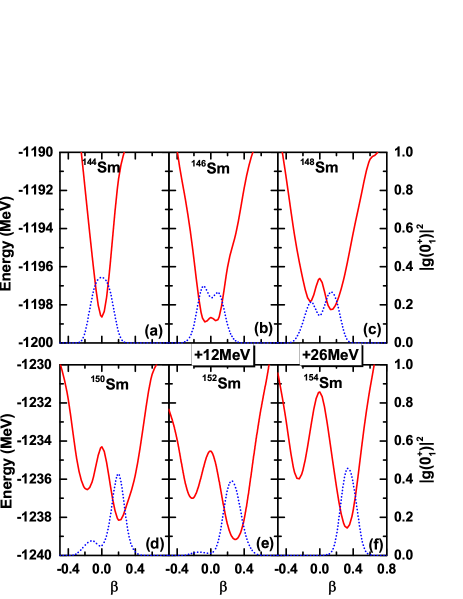
Figure 1: The total energy in the mean-field approximation for Sm isotopes as a function of the the intrinsic quadrupole deformation $\beta$ (the solid lines). The energy curves for ¹⁴⁶Sm and ¹⁵²Sm are shifted upward by 12 MeV, while those for ¹⁴⁸Sm and ¹⁵⁴Sm are shifted by 26 MeV. The square of the collective wave functions, $|g_{nI}(\beta)|^{2}$, for the GCM ground states ($0_{1}^{+}$) are also shown with the dashed curves.

Before we discuss the structure of the hypernuclei, we first discuss the structure of the core nuclei. The solid lines in Fig. 1 show the total mean-field energy for the ^144-154Sm nuclei as a function of the quadrupole deformation parameter, $\beta$. For the ¹⁴⁴Sm nucleus, one can see that the potential energy curve is almost parabolic centered at the spherical shape. As the neutron number increases, the energy curve gradually presents two pronounced minima, located on the oblate and the prolate sides, respectively. A previous study Li et al. (2009) has shown that these two minima are connected with a tunneling along the trixiality (that is, a $\gamma$ deformation). In other words, the oblate minimum is actually a saddle point on the energy surface. The true energy minimum is thus the prolate one, that shifts gradually towards a large $\beta$ as the neutron number increases, from $\beta=0.08$ for ¹⁴⁸Sm to $\beta=0.32$ for ¹⁵⁴Sm.

The square of the collective wave function, $|g_{nI}(\beta)|^{2}$, for the ground state ($0^{+}_{1}$) of each isotope is shown by the dashed lines in the figure. Here, the collective wave function is defined as Ring and Schuck (1980),

$$g_{nI}(\beta)\equiv\sum_{\beta^{\prime}}\big{[}\mathcal{N}^{I}\big{]}^{1/2}(\beta,\beta^{\prime})F_{nI}(\beta^{\prime}),$$ (8)

where the norm kernel is given as $\mathcal{N}^{I}(\beta,\beta^{\prime})\equiv\langle\beta|\hat{P}^{I}\hat{P}^{N}\hat{P}^{Z}|\beta^{\prime}\rangle$. Notice that the weight function $F_{nI}(\beta)$ in Eq. (2) cannot be interpreted as a probability amplitude due to the non-orthgonality of the reference wave functions. The figure clearly indicates that the predominant component in the ground state changes gradually from the spherical configuration in ¹⁴⁴Sm to the prolate deformed one in ¹⁵⁴Sm.

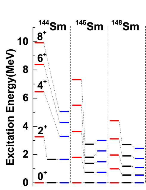
Figure 2: The yrast levels of the Sm isotopes calculated with the MR-CDFT (the red lines) in comparison to the experiment data (the black lines) taken from Ref. NND . The figure also shows the scaled levels (the blue lines) with a multiplicative factor of $f=E^{\mathrm{exp}.}_{2^{+}}/E^{\mathrm{MR-CDFT}}_{2^{+}}$, that is $E^{\mathrm{Scaled}}_{I^{+}}=f\cdot E^{\mathrm{MR-CDFT}}_{I^{+}}$.

Figure 2 shows calculated energy spectra for the lowest $0^{+}$, $2^{+}$, $4^{+}$, $6^{+}$, and $8^{+}$ states in the Sm isotopes, in comparison to the corresponding data. As one can see, the main characters of the energy spectra are reasonably reproduced in this calculation, although the excitation energies are somewhat overestimated. In fact, the energy spectra become close to the data, as shown in the figure, after all the excitation energies are scaled so that the experimental energy is reproduced for the first $2^{+}$ state.

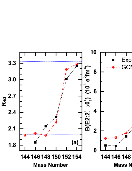
Figure 3: (a) The ratio $R_{4/2}$ of the excitation energy for the first 4⁺ state to that for the first 2⁺ state for the Sm isotopes as a function of the mass number. (b) The electromagnetic transition strength, in units $10^{3}\,e^{2}$fm⁴, from the first 2⁺ state to the ground state, $B(E2:2^{+}_{1}\rightarrow 0^{+}_{1})$, as a function of the mass number for the Sm isotopes. The experiment data are taken from Ref. NND .

In literature, the energy ratio, $R_{4/2}\equiv E(4^{+}_{1})/E(2^{+}_{1})$, of the excitation energy for the $4^{+}_{1}$ state to that for the $2^{+}_{1}$ state has often been adopted to characterize nuclear collective excitations. This value for ¹⁴⁴Sm, ¹⁴⁶Sm and ¹⁴⁸Sm is $R_{4/2}=1.98$, $2.01$ and $1.98$, respectively, all of which are close to the value in the harmonic oscillator limit, $R_{4/2}=2.0$. With the increase of the neutron number, the value of $R_{4/2}$ increases up to 3.29 for ¹⁵⁴Sm, that is close to the value in the rigid rotor limit, $R_{4/2}=3.33$. Figure 3(a) illustrates this transition. The figure clearly demonstrates that the theoretical results present shape transition from spherical to deformed in the Sm isotopes around $N=90$, which is in good agreement with the experimental data. This picture is verified also from the mass number dependence of the electric quadrupole transition strength from the first 2⁺ state to the ground state, $B(E2;2^{+}_{1}\rightarrow 0^{+}_{1})$, as shown in Fig. 3(b).

III.2 Low-lying spectrum of _ΛSm isotopes

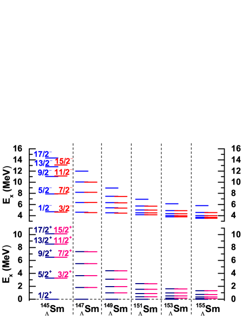
Figure 4: The spectrum for the first positive parity states in the _ΛSm isotopes. The location of the spin doublet states are arranged based on the yrast levels of the even Sm core nuclei.

Table 1: The probability $P$ of the dominant components, defined as $P\equiv\int drr^{2}|{\mathscr{R}}_{j\ell nI}(r)|^{2}$, in the wave functions for the positive-parity states.

$J^{\pi}$	$(lj)\otimes I^{\pi}_{n}$	${}^{145}_{~{}~{}\Lambda}$Sm	${}^{147}_{~{}~{}\Lambda}$Sm	${}^{149}_{~{}~{}\Lambda}$Sm	${}^{151}_{~{}~{}\Lambda}$Sm	${}^{153}_{~{}~{}\Lambda}$Sm	${}^{155}_{~{}~{}\Lambda}$Sm
$1/2^{+}_{1}$	$s_{1/2}\otimes 0_{1}^{+}$	$0.998$	$0.998$	$0.997$	$0.994$	$0.988$	$0.982$
$3/2^{+}_{1}$	$s_{1/2}\otimes 2_{1}^{+}$	$0.997$	$0.997$	$0.996$	$0.993$	$0.988$	$0.982$
$5/2^{+}_{1}$	$s_{1/2}\otimes 2_{1}^{+}$	$0.997$	$0.997$	$0.996$	$0.993$	$0.988$	$0.982$
$7/2^{+}_{1}$	$s_{1/2}\otimes 4_{1}^{+}$	$0.991$	$0.996$	$0.996$	$0.993$	$0.987$	$0.982$
$1/2^{+}_{2}$	$s_{1/2}\otimes 0_{2}^{+}$	$0.987$	$0.983$	$0.993$	$0.992$	$0.987$	$0.990$
$3/2^{+}_{2}$	$s_{1/2}\otimes 2_{2}^{+}$	$0.981$	$0.996$	$0.995$	$0.992$	$0.986$	$0.989$
$5/2^{+}_{2}$	$s_{1/2}\otimes 2_{2}^{+}$	$0.980$	$0.996$	$0.995$	$0.991$	$0.986$	$0.989$
$7/2^{+}_{2}$	$s_{1/2}\otimes 4_{2}^{+}$	$0.988$	$0.993$	$0.994$	$0.987$	$0.985$	$0.986$

We now discuss the low-lying states in the _ΛSm hypernuclei, in which a $\Lambda$ particle couples to the core states presented in the previous subsection. Figure 4 shows the calculated yrast positive-parity states in the _ΛSm isotopes. The probability for the dominant configuration in the wave function for the $1/2^{+}$, $3/2^{+}$, $5/2^{+}$, and $7/2^{+}$ states is also presented in Table 1. These positive-parity states are dominated by the configuration of $[\Lambda_{s_{1/2}}\otimes I^{+}_{1}]$ with the weight around $99\%$, where $\Lambda_{s_{1/2}}$ denotes the $\Lambda$ particle in the $s_{1/2}$ configuration. They are nontrivial results obtained for all the _ΛSm isotopes. These states have a similar excitation energy to that of the nuclear core state with $I^{+}_{1}$, and are nearly two-fold degenerate except for the $1/2^{+}_{1}$ state. These characters are similar to hypernuclei in the light-mass region, and are also consistent with our previous calculation for ${}^{155}_{~{}~{}\Lambda}$Sm with a simplified $\Lambda N$ interaction Mei et al. (2015).

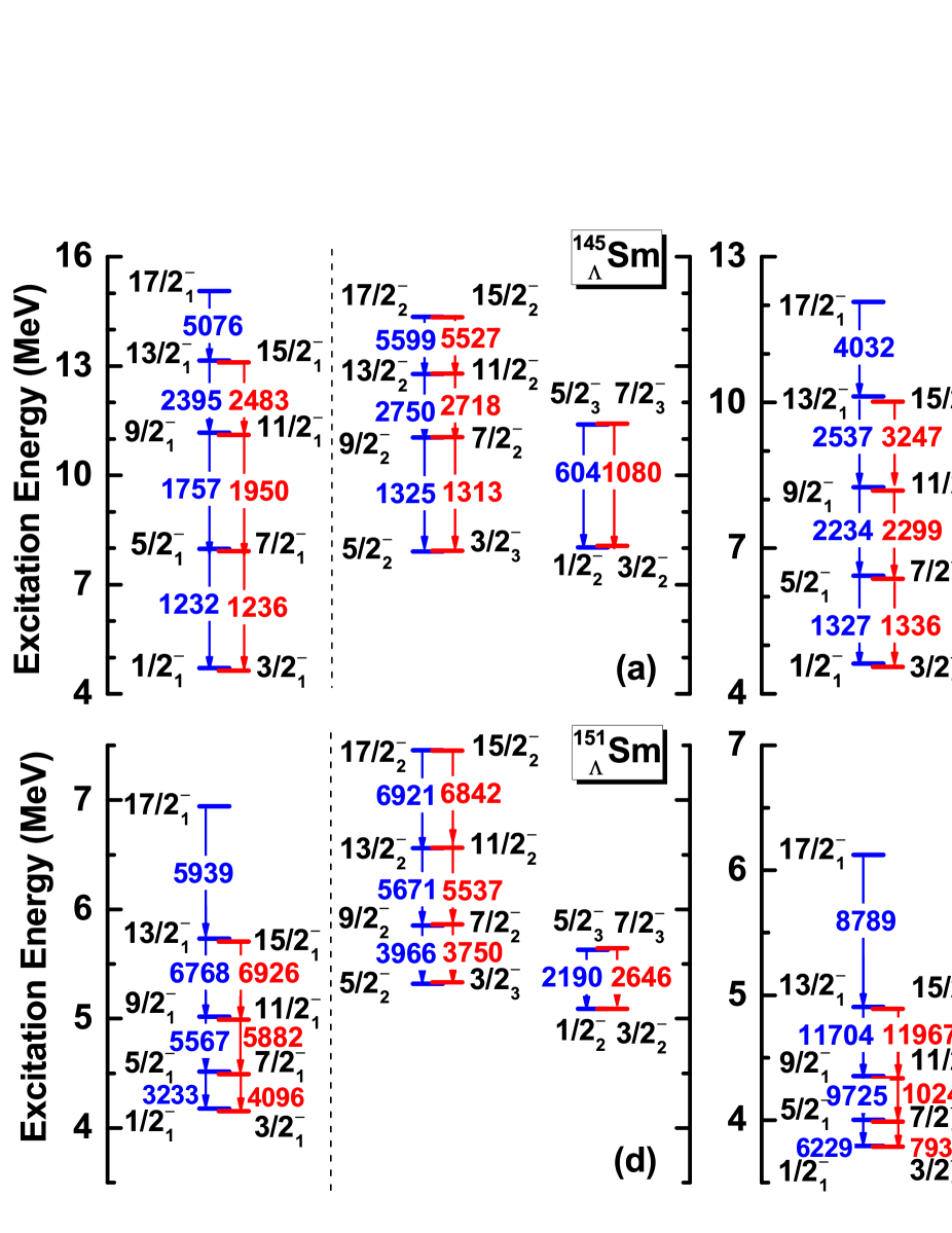
Figure 5: The low-lying negative-parity states in the _ΛSm isotopes obtained with the microscopic particle-core coupling scheme based on the covariant density functional theory. The arrows indicate the E2 transition strengths, given in units of $e^{2}$ fm⁴.

Table 2: Same as Table 1, but for the negative-parity states shown in Fig. 5. The blank entries indicate the probabilities smaller than $0.001$.

$J^{\pi}$	$(lj)\otimes I^{\pi}_{n}$	${}^{145}_{~{}~{}\Lambda}$Sm	${}^{147}_{~{}~{}\Lambda}$Sm	${}^{149}_{~{}~{}\Lambda}$Sm	${}^{151}_{~{}~{}\Lambda}$Sm	${}^{153}_{~{}~{}\Lambda}$Sm	${}^{155}_{~{}~{}\Lambda}$Sm
$1/2^{-}_{1}$	$p_{1/2}\otimes 0_{1}^{+}$	$0.986$	$0.964$	$0.859$	$0.484$	$0.348$	$0.322$
	$p_{3/2}\otimes 2_{1}^{+}$	$0.012$	$0.033$	$0.136$	$0.503$	$0.627$	$0.639$
$3/2^{-}_{1}$	$p_{1/2}\otimes 2_{1}^{+}$	$0.006$	$0.015$	$0.054$	$0.204$	$0.271$	$0.281$
	$p_{3/2}\otimes 0_{1}^{+}$	$0.986$	$0.965$	$0.876$	$0.545$	$0.395$	$0.363$
	$p_{3/2}\otimes 2_{1}^{+}$	$0.006$	$0.017$	$0.064$	$0.238$	$0.309$	$0.318$
$5/2^{-}_{1}$	$p_{1/2}\otimes 2_{1}^{+}$	$0.980$	$0.959$	$0.573$	$0.453$	$0.385$	$0.346$
	$p_{3/2}\otimes 4_{1}^{+}$	$0.012$	$0.034$	$0.154$	$0.377$	$0.462$	$0.504$
	$p_{3/2}\otimes 2_{1}^{+}$			$0.262$	$0.156$	$0.127$	$0.112$
$7/2^{-}_{1}$	$p_{1/2}\otimes 4_{1}^{+}$	$0.008$	$0.022$	$0.074$	$0.183$	$0.232$	$0.258$
	$p_{3/2}\otimes 2_{1}^{+}$	$0.980$	$0.954$	$0.854$	$0.653$	$0.554$	$0.497$
	$p_{3/2}\otimes 4_{1}^{+}$	$0.006$	$0.018$	$0.062$	$0.150$	$0.188$	$0.207$
$9/2^{-}_{1}$	$p_{1/2}\otimes 4_{1}^{+}$	$0.843$	$0.931$	$0.570$	$0.481$	$0.398$	$0.372$
	$p_{3/2}\otimes 4_{1}^{+}$	$0.071$	$0.016$	$0.288$	$0.210$	$0.166$	$0.154$
	$p_{3/2}\otimes 6_{1}^{+}$	$0.040$	$0.033$	$0.131$	$0.295$	$0.407$	$0.437$
$1/2^{-}_{2}$	$p_{1/2}\otimes 0_{1}^{+}$	$0.013$	$0.035$	$0.133$	$0.498$	$0.635$	$0.654$
	$p_{3/2}\otimes 2_{1}^{+}$	$0.978$	$0.945$	$0.813$	$0.472$	$0.351$	$0.330$
$3/2^{-}_{2}$	$p_{1/2}\otimes 2_{1}^{+}$	$0.734$	$0.655$	$0.272$	$0.210$	$0.136$	$0.119$
	$p_{3/2}\otimes 2_{1}^{+}$	$0.246$	$0.295$	$0.583$	$0.322$	$0.266$	$0.258$
	$p_{3/2}\otimes 0_{1}^{+}$	$0.012$	$0.031$	$0.113$	$0.435$	$0.583$	$0.605$
$5/2^{-}_{2}$	$p_{1/2}\otimes 2_{1}^{+}$			$0.283$	$0.221$	$0.210$	$0.202$
	$p_{3/2}\otimes 2_{1}^{+}$	$0.988$	$0.978$	$0.658$	$0.746$	$0.764$	$0.780$
$7/2^{-}_{2}$	$p_{1/2}\otimes 4_{1}^{+}$	$0.261$	$0.240$	$0.580$	$0.497$	$0.478$	$0.484$
	$p_{3/2}\otimes 4_{1}^{+}$	$0.695$	$0.726$	$0.205$	$0.486$	$0.492$	$0.499$
	$p_{3/2}\otimes 2_{2}^{+}$	$0.014$		$0.139$
$9/2^{-}_{2}$	$p_{1/2}\otimes 4_{1}^{+}$	$0.083$	$0.013$	$0.303$	$0.281$	$0.263$	$0.265$
	$p_{3/2}\otimes 4_{1}^{+}$	$0.888$	$0.943$	$0.619$	$0.703$	$0.707$	$0.719$
$3/2^{-}_{3}$	$p_{1/2}\otimes 2_{1}^{+}$	$0.253$	$0.313$	$0.636$	$0.553$	$0.571$	$0.579$
	$p_{3/2}\otimes 2_{1}^{+}$	$0.741$	$0.672$	$0.304$	$0.416$	$0.402$	$0.401$
$5/2^{-}_{3}$	$p_{1/2}\otimes 2_{1}^{+}$	$0.007$	$0.034$	$0.123$	$0.313$	$0.389$	$0.429$
	$p_{3/2}\otimes 4_{1}^{+}$	$0.712$	$0.759$	$0.724$	$0.609$	$0.514$	$0.464$
$7/2^{-}_{3}$	$p_{1/2}\otimes 4_{1}^{+}$	$0.527$	$0.476$	$0.302$	$0.307$	$0.266$	$0.237$
	$p_{3/2}\otimes 4_{1}^{+}$	$0.251$	$0.132$	$0.368$	$0.350$	$0.294$	$0.272$
	$p_{3/2}\otimes 2_{2}^{+}$	$0.116$	$0.269$	$0.137$
	$p_{3/2}\otimes 2_{1}^{+}$	$0.010$	$0.033$	$0.124$	$0.336$	$0.428$	$0.472$

In the negative parity states of _ΛSm isotopes, novel and interesting features are disclosed. The low-lying negative-parity states are shown in Fig. 5. We summarize in Table 2 the dominant components in the wave functions for a few selected levels. One can see that these negative-parity states are formed mainly from a $\Lambda$-particle in $p$ orbitals coupled to core states, and are nearly two-fold degenerate. The E2 transition strengths between the negative parity states are also shown in the figure. The ratio of the $E2$ transition strength for the transition $5/2_{1}^{-}\rightarrow 1/2_{1}^{-}$ to that for $9/2_{1}^{-}\rightarrow 5/2_{1}^{-}$ is 0.641 and 0.695 in ${}^{153}_{~{}~{}\Lambda}$Sm and ${}^{155}_{~{}~{}\Lambda}$Sm, respectively. These values are both close to 0.7, that is the ratio of the $E2$ transition strength for $2^{+}\rightarrow 0^{+}$ to that for $4^{+}\rightarrow 2^{+}$ in the $K=0$ ground-state rotational band of well-deformed nuclei Ring and Schuck (1980). A simple relation among the $B(E2)$ values for the negative-parity bands in a well deformed hypernucleus is further discussed in Appendix A.

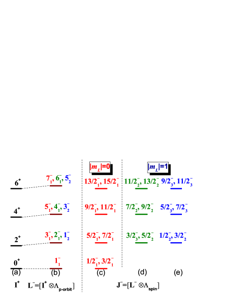
Figure 6: A schematic picture for hypernuclear states based on the $LS$ coupling scheme. It is assumed that a $\Lambda$-particle is in a $p$-orbital and coupled to spherical core states.

The level structure of the negative-parity states shown in Fig. 5 can be understood in terms of the $LS$ coupling scheme. To demonstrate this, let us consider a simplified situation in which the core states with $K=0$ shown in Fig.  6 (a) are coupled to a $\Lambda$ particle in $p$ orbitals. We first couple the core angular momentum $I$ with the orbital angular momentum of the $\Lambda$ particle, $l_{\Lambda}=1$. This results in the levels shown in Fig. 6 (b). These levels may be categorized according to the projection of the total orbital angular momentum, $\mbox{\boldmath$L$}=\mbox{\boldmath$I$}+\mbox{\boldmath$l$}_{\Lambda}$, on to the symmetric axis, that is, $m_{L}=K+m_{\Lambda}$. Since $K$=0, there are two possibilities for $|m_{L}|$, that is, $m_{L}=0$ and $\pm 1$. The levels with $m_{L}=0$ form a band with $1_{1}^{-},3_{1}^{-},5_{1}^{-},7_{1}^{-},\cdots$, while the levels with $m_{L}=\pm 1$ form another band with $1_{2}^{-},2_{1}^{-},3_{2}^{-},4_{1}^{-},\cdots$. If one further couples the spin 1/2 of the $\Lambda$ particle to these rotational bands, one obtains the levels in Fig. 6 (c) for the $m_{L}=0$ band, and the levels in Figs. 6 (d) and (e) for the $m_{L}=\pm 1$ band. For a given $I$, the levels belonging to the $m_{L}=0$ and the $m_{L}=\pm 1$ bands are degenerate in energy for spherical hypernuclei. For prolately deformed hypernuclei, on the other hand, the level in the $m_{L}=0$ band is lower in energy than the levels in the $m_{L}=\pm 1$ band because the former configuration gains more energy due to a better overlap with the core nucleus. This feature explain well the energy relation among the three doublet states of (5/2${}_{1}^{-}$, 7/2${}_{1}^{-}$), (3/2${}_{2}^{-}$, 5/2${}_{2}^{-}$), and (1/2${}_{2}^{-}$, 3/2${}_{2}^{-}$) in, e.g., ${}^{145}_{~{}~{}\Lambda}$Sm and ${}^{155}_{~{}~{}\Lambda}$Sm (see Fig. 5).

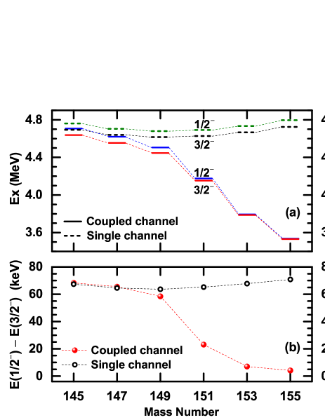
Figure 7: (a) The energy levels of the $1/2^{-}_{1}$ and $3/2^{-}_{1}$ states in the _ΛSm hypernuclei as a function of the mass number. The solid line and the dashed line indicate the results of the coupled-channels and the single-channel calculations, respectively. (b) The energy splitting between the $1/2^{-}_{1}$ and $3/2^{-}_{1}$ states shown in the upper panel.

Figure 7(a) shows in details the excitation energy of the lowest $1/2^{-}_{1}$ and $3/2^{-}_{1}$ states in the _ΛSm isotopes as a function of the neutron number. The dashed energy levels show the results of the single-channel calculations, for which the sum in Eq. (3) is restricted only to a single configuration. For the lowest $1/2^{-}_{1}$ and $3/2^{-}_{1}$ states, the configuration in the single-channel calculation is a pure configuration of $[\Lambda p_{1/2}\otimes 0^{+}_{1}]$ and $[\Lambda p_{3/2}\otimes 0^{+}_{1}]$, respectively. Their excitation energies are around 4.8 MeV for all the hypernuclei considered in this paper, which is close to the energy $\frac{2}{3}\times 41A^{-1/3}\sim 5.14$ MeV with $A\sim 150$ for exciting one hyperon from $s$ orbit to $p$ orbit. The energy difference between these states remains around 70 keV, as shown by the open circles in Figure 7(b). In marked contrast, the energy of the $1/2^{-}_{1}$ and $3/2^{-}_{1}$ states obtained by including the configuration mixing effect decreases continuously from 4.7 MeV to 3.5 MeV as the neutron number increases from 82 to 92 (see the solid lines in Fig. 7(a)). The splitting of these two states also decreases from 68 keV to 4 keV, as shown in Fig. 7(b) by the filled circles. The deviation from the single-channel calculations increases as the core nucleus undergoes phase transition from a spherical vibrator to a well-deformed rotor, indicating a stronger configuration mixing effect in deformed hypernuclei.

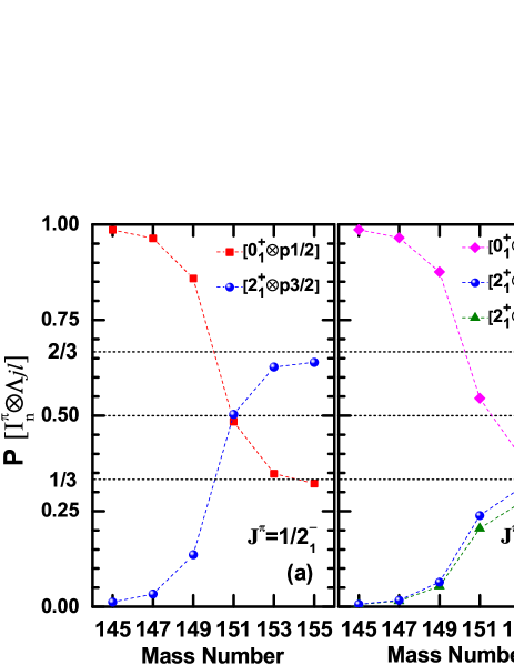
Figure 8: The probability $P_{k}$ for the dominant components in the wave function of (a) the $1/2^{-}_{1}$ state and (b) the $3/2^{-}_{1}$ state as a function of the mass number of the _ΛSm isotopes.

This feature can be seen also in the compositions of the wave functions listed in Table 2. In ${}^{145}_{~{}~{}\Lambda}$Sm(${}^{147}_{\Lambda}$Sm), the $1/2^{-}_{1}$ and $3/2^{-}_{1}$ states are almost pure configuration of $[\Lambda p_{1/2}\otimes 0^{+}_{1}]$ and $[\Lambda p_{3/2}\otimes 0^{+}_{1}]$, respectively. This is consistent with the fact that the single-channel calculation works well for this hypernucleus (see Fig. 7). With the increase of the neutron number, the mixing between the $[\Lambda p_{1/2}\otimes 0^{+}_{1}]$ and $[\Lambda p_{3/2}\otimes 2^{+}_{1}]$ configurations in the $1/2^{-}_{1}$ state becomes stronger and reaches the largest value in ${}^{155}_{~{}~{}\Lambda}$Sm. This feature is shown clearly in Fig. 8(a). One can see that the mixing between $0^{+}_{1}$ and $2^{+}_{1}$ becomes almost half-and-half in ${}^{151}_{~{}~{}\Lambda}$Sm. In the well-deformed ${}^{155}_{~{}~{}\Lambda}$Sm, the weight for the $[\Lambda p_{1/2}\otimes 0_{1}^{+}]$ configuration becomes 32.2% while that for the $[\Lambda p_{3/2}\otimes 2_{1}^{+}]$ configuration becomes 63.9%. For the $3/2^{-}_{1}$ state, on the other hand, the wave function shows a mixture of the $[\Lambda p_{3/2}\otimes 0_{1}^{+}]$, $[\Lambda p_{1/2}\otimes 2_{1}^{+}]$ and $[\Lambda p_{3/2}\otimes 2_{1}^{+}]$ configurations. The mass number dependence of the weight factors is shown in Fig. 8(b), indicating a similar feature as in the $1/2_{1}^{-}$ state. That is, the configuration mixing becomes stronger as the core nucleus undergoes a transition from spherical to deformed. For the ${}^{155}_{~{}~{}\Lambda}$Sm hypernucleus, the weight factors are 36.3%, 28.1%, and 31.8%, for the $[\Lambda p_{3/2}\otimes 0_{1}^{+}]$, $[\Lambda p_{1/2}\otimes 2_{1}^{+}]$ and $[\Lambda p_{3/2}\otimes 2_{1}^{+}]$ configurations, respectively.

It is worth mentioning that for all the negative-parity states in the $m_{L}=0$ band of ${}^{155}_{~{}~{}\Lambda}$Sm shown in Table 2, the weight for the configurations with $p_{1/2}$ is around 33%, while a sum of the weight factors for the configurations with $p_{3/2}$ is close to 67%. To understand this, let us employ the Nilsson model for the hyperon with an axially deformed potential, $V(\mbox{\boldmath$r$})=V_{0}(r)-\beta R_{0}\frac{dV_{0}(r)}{dr}Y_{20}(\hat{\mbox{\boldmath$r$}})$. Notice that, with this deformed potential, several orbital angular momenta $l$ and total angular momenta $j$ are mixed in the hyperon wave function. Treating the deformed part of the potential, $-\beta R_{0}\frac{dV_{0}(r)}{dr}Y_{20}(\hat{\mbox{\boldmath$r$}})$, with the first order perturbation theory and neglecting the mixture across two major shells, one can write the wave function for the lowest negative parity state as $|\psi_{\Lambda}\rangle=C_{1}|p3/2,1/2\rangle+C_{2}|p1/2,1/2\rangle$, where $|p3/2,1/2\rangle$ and $|p1/2,1/2\rangle$ are single-particle wave functions in the spherical limit with $j_{z}=1/2$. The coefficients $C_{1}$ and $C_{2}$ are simply determined by the following eigenvalue equation,

$$\left(\begin{array}[]{cc}\langle\mathscr{Y}_{p3/2,1/2}|Y_{20}|\mathscr{Y}_{p3/2,1/2}\rangle&\langle\mathscr{Y}_{p3/2,1/2}|Y_{20}|\mathscr{Y}_{p1/2,1/2}\rangle\\ \langle\mathscr{Y}_{p1/2,1/2}|Y_{20}|\mathscr{Y}_{p3/2,1/2}\rangle&\langle\mathscr{Y}_{p1/2,1/2}|Y_{20}|\mathscr{Y}_{p1/2,1/2}\rangle\\ \end{array}\right)$$ (11)

$$\times\left(\begin{array}[]{c}C_{1}\\ C_{2}\\ \end{array}\right)=\lambda\left(\begin{array}[]{c}C_{1}\\ C_{2}\\ \end{array}\right).$$ (16)

The value of the matrix elements $\displaystyle\langle\mathscr{Y}_{p3/2,1/2}|Y_{20}|\mathscr{Y}_{p3/2,1/2}\rangle$, $\displaystyle\langle\mathscr{Y}_{p3/2,1/2}|Y_{20}|\mathscr{Y}_{p1/2,1/2}\rangle$, $\displaystyle\langle\mathscr{Y}_{p1/2,1/2}|Y_{20}|\mathscr{Y}_{p3/2,1/2}\rangle$ and $\displaystyle\langle\mathscr{Y}_{p1/2,1/2}|Y_{20}|\mathscr{Y}_{p1/2,1/2}\rangle$ is $\displaystyle\frac{1}{\sqrt{20\pi}}$, $\displaystyle-\dfrac{2}{\sqrt{20\pi}}$, $\displaystyle-\frac{2}{\sqrt{20\pi}}$ and 0, respectively. The solutions of Eq.(11) then give two eigenvectors, $\displaystyle(C_{1},C_{2})^{T}=(\sqrt{2/3},-\sqrt{1/3})^{T}$ and $\displaystyle(\sqrt{1/3},\sqrt{2/3})^{T}$, with the eigenvalues of $\displaystyle\lambda=2/\sqrt{20\pi}$ and $\displaystyle-1/\sqrt{20\pi}$, respectively. For a positive value of $\beta$, the former state is lower in energy. For this state, the probability of the $p_{3/2}$ component reads 66.7% and that of $p_{1/2}$ component is 33.3%. This clearly implies that the weight factors shown in Table 2 are consistent with the Nilsson model and thus can be understood in terms of the strong coupling limit of the particle-rotor model.

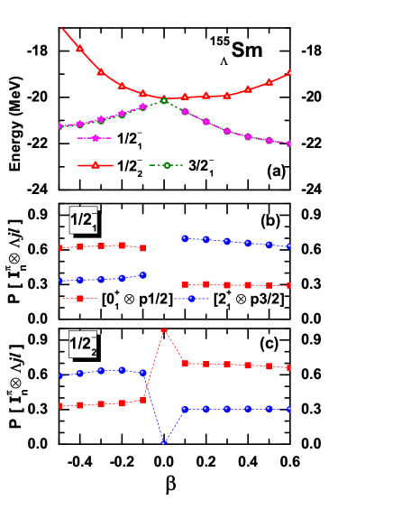
Figure 9: (a) The energy of the $J^{\pi}=1/2^{-}_{1},1/2^{-}_{2}$ and $3/2^{-}_{1}$ states of the ${}^{155}_{~{}~{}\Lambda}$Sm hypernucleus as a function of the quadrupole deformation $\beta$ of the core nucleus. These curves are obtained with the microscopic particle-rotor model calculation by setting the excitation energies of the core states to be zero. (b) The probability $P_{k}$ of the dominant components in the $1/2^{-}_{1}$ state as a function of the deformation parameter, $\beta$. (c) Same as (b), but for the $1/2^{-}_{2}$ state.

In addition, we also carry out the coupled-channels calculation for ${}^{155}_{~{}~{}\Lambda}$Sm by setting the excitation energies of the nuclear core states to be zero. In order to draw the energy curve as a function of the deformation parameter, we take $F_{nI}(\beta)=\delta_{\beta,\beta^{\prime}}$ in Eq. (2) and compute the total energy for $\beta=\beta^{\prime}$ Xue et al. (2015). Notice that this is a reasonable approximation for well-deformed hypernuclei. The calculated energy for the $1/2^{-}_{1},1/2^{-}_{2}$ and $3/2^{-}_{1}$ states are shown in Fig. 9(a). The splitting of the single-particle states due to nuclear deformation is a well known feature of the Nilsson diagram Ring and Schuck (1980). The main components of the wave function are shown in Figs.  9(b) and (c) for the $1/2_{1}^{-}$ and $1/2_{2}^{-}$ states, respectively. One can see that the $1/2^{-}_{1}$ state composes mainly of the $[\Lambda p_{1/2}\otimes 0_{1}^{+}]$ and $[\Lambda p_{3/2}\otimes 2_{1}^{+}]$ configurations with a rather constant mixing weight of around 30% and 70%, respectively, on the prolate side. The mixing weights for these two configurations are exchanged on the oblate side. The mixing weights for the $1/2^{-}_{2}$ state are just opposite to those for the $1/2^{-}_{1}$ state. These findings confirm the analysis based on the simple Nilsson potential presented in the previous paragraph.

IV Summary

We have systematically investigated the configuration mixing in low-lying states of Sm hypernuclei using the microscopic particle-core coupling scheme based on the covariant density functional theory. We emphasize that this is the first microscopic calculation for hypernuclear spectra in (medium-)heavy hypernuclei and can be achieved only with the mean-field based calculations, in which the beyond-mean-field correlations are also included. We have found that the positive-parity ground-state band shares a similar structure to that for the core nucleus. That is, the hypernuclear states with spin-parity of $(I\pm 1/2)^{+}$ are dominated by the configuration of $[\Lambda s_{1/2}\otimes I^{+}]$, where $\Lambda s_{1/2}$ denotes the $\Lambda$ particle in the $s_{1/2}$ state, regardless of whether the core nucleus is spherical or deformed. In contrast, the low-lying negative-parity states show an admixture of the $\Lambda p_{1/2}$ and the $\Lambda p_{3/2}$ configurations coupled with nuclear core states having $I$ and $I\pm 2$. We have shown that the mixing amplitude is negligibly small in spherical and weakly-deformed nuclei, while it becomes increasingly stronger as the core nucleus undergoes a shape transition to a well-deformed shape. We have demonstrated that the energy spectra for low-lying negative parity states in Sm hypernuclei can be well understood with the $LS$ coupling scheme with the orbital angular momentum of $L=|I-1|,I,I+1$ and the spin angular momentum of $S=1/2$. For well-deformed hypernuclei, the spectra as well as the wave functions are also consistent with the Nilsson model.

The conclusion obtained in this paper can be applied to hypernuclei in any mass region, provided that the low-lying states of the core nucleus are dominated by quadrupole collective excitations. This indicates that the spin-orbit splitting for the hyperon $p$-orbital should be estimated from the energy difference between the first $1/2^{-}$ and $3/2^{-}$ states in hypernuclei with a nearly spherical nuclear core.

Appendix A $E2$ transition strengths in a well deformed hypernucleus

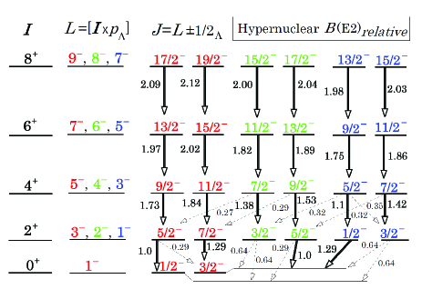
Figure 10: The relation among the $E2$ transition strengths for transition between low-lying negative parity states in a well deformed hypernucleus. The solid line indicates strong transitions, for which the $B(E2)$ value is larger than the $B(E2)$ value for the transition from the first excited state with $(I,L,J)=(2,3,5/2)$ to the ground state with $(I,L,J)=(0,1,1/2)$, where $I$, $L$, and $J$ are the spin of the core nucleus, the total orbital angular momentum of the hypernuclei and the total spin of the hypernuclei, respectively. The dashed lines denote weaker transitions. See Table 3 for the actual values of the transition strengths. We note that the band with $m_{L}=0$ should be lower in energy than the other two with $m_{L}=\pm 1$ for a well-deformed hypernucleus, as we have discussed in Figs. 5 and 6.

Table 3: The $E2$ transition strengths for transition between low-lying negative parity states in a well deformed hypernucleus. The $B(E2)$ values are given relative to the value for the transition from the first excited state with $(I,L,J)=(2,3,5/2)$ to the ground state with $(I,L,J)=(0,1,1/2)$, where $I$, $L$, and $J$ are the spin of the core nucleus, the total orbital angular momentum of the hypernuclei and the total spin of the hypernuclei, respectively. Only the $B(E2)$ values larger than 0.25 are listed.

$I_{i}$	$L_{i}$	$J_{i}$	$I_{f}$	$L_{f}$	$J_{f}$	$B(E2:J_{i}\to J_{f})$
2	3	5/2	0	1	1/2	1.00
2	3	5/2	0	1	3/2	0.286
2	3	7/2	0	1	3/2	1.29
2	2	3/2	0	1	1/2	0.643
2	2	3/2	0	1	3/2	0.643
2	2	5/2	0	1	1/2	0.286
2	2	5/2	0	1	3/2	1.00
2	1	1/2	0	1	3/2	1.29
2	1	3/2	0	1	1/2	0.643
2	1	3/2	0	1	3/2	0.643
4	5	9/2	2	3	5/2	1.73
4	5	11/2	2	3	7/2	1.84
4	4	7/2	2	3	5/2	0.273
4	4	9/2	2	3	7/2	0.289
4	4	7/2	2	2	3/2	1.38
4	4	9/2	2	2	5/2	1.53
4	3	5/2	2	2	3/2	0.315
4	3	7/2	2	2	5/2	0.354
4	3	5/2	2	1	1/2	1.10
4	3	5/2	2	1	3/2	0.315
4	3	7/2	2	1	3/2	1.42
6	7	13/2	4	5	9/2	1.97
6	7	15/2	4	5	11/2	2.02
6	6	11/2	4	4	7/2	1.82
6	6	13/2	4	4	9/2	1.89
6	5	9/2	4	3	5/2	1.75
6	5	11/2	4	3	7/2	1.86

In this Appendix, we derive a simple expression for the $B(E2)$ values for the $E2$ transition between the negative-parity states in a well deformed hypernucleus. To this end, we use the $LS$ coupling scheme discussed in Sec. III.2 and consider a transition from the initial state $|J_{i}M_{i}\rangle$ to the final state $|J_{f}M_{f}\rangle$, whose wave function is given by

$$|J_{i}M_{i}\rangle=\left|\left[[I_{i}\otimes l_{\Lambda}]^{(L_{i})}\otimes s_{\Lambda}\right]^{(J_{i}M_{i})}\right\rangle,$$ (17)

$$|J_{f}M_{f}\rangle=\left|\left[[I_{f}\otimes l_{\Lambda}]^{(L_{f})}\otimes s_{\Lambda}\right]^{(J_{f}M_{f})}\right\rangle,$$ (18)

respectively. Here, $I_{i}$ and $I_{f}$ are the initial and the final spin of the core nucleus, respectively, and $s_{\Lambda}=1/2$ is the spin of the $\Lambda$ particle. We assume that the initial and the final states are dominated by configurations with the $\Lambda$ particle in the $p$ orbits, and we take the orbital angular momentum of the $\Lambda$ particle to be $l_{\Lambda}=1$.

The $E2$ transition operator, $\hat{T}_{2}$, acts only on the core states. Using Eq. (7.1.7) in Ref. Edmonds (1957), the reduced matrix element of the $E2$ operator between the initial and the final states reads,

$$\langle J_{f}||\hat{T}_{2}||J_{i}\rangle = (-1)^{L_{f}+\frac{1}{2}+J_{i}+2}\,\hat{J_{i}}\hat{J_{f}}\left\{\begin{array}[]{ccc}L_{f}&J_{f}&1/2\\ J_{i}&L_{2}&2\end{array}\right\}$$ (25)

$$\times(-1)^{I_{f}+l_{\Lambda}+L_{i}+2}\,\hat{L_{i}}\hat{L_{f}}\left\{\begin{array}[]{ccc}I_{f}&L_{f}&l_{\Lambda}\\ L_{i}&I_{i}&2\end{array}\right\}$$

$$\times\langle I_{f}||\hat{T}_{2}||I_{i}\rangle.$$

Here, we have used a shorthanded notation of $\hat{J}\equiv\sqrt{2J+1}$. The $B(E2)$ value for the transition from the initial to the final states is then given as

$$B(E2;J_{i}\to J_{f}) = \frac{1}{2J_{i}+1}\,|\langle J_{f}||\hat{T}_{2}||J_{i}\rangle|^{2},$$ (32)

$$= (2J_{f}+1)(2L_{i}+1)(2L_{f}+1)$$

$$\times\left\{\begin{array}[]{ccc}L_{f}&J_{f}&1/2\\ J_{i}&L_{i}&2\end{array}\right\}^{2}\left\{\begin{array}[]{ccc}I_{f}&L_{f}&l_{\Lambda}\\ L_{i}&I_{i}&2\end{array}\right\}^{2}$$

$$\times|\langle I_{f}||\hat{T}_{2}||I_{i}\rangle|^{2}.$$

Notice that $|\langle I_{f}||\hat{T}_{2}||I_{i}\rangle|^{2}$ in the last line is related to the $B(E2)$ value for the core transition as $|\langle I_{f}||\hat{T}_{2}||I_{i}\rangle|^{2}=(2I_{i}+1)\,B(E2;I_{i}\to I_{f})$. In order to evaluate it, we use the collective model Ring and Schuck (1980), that is,

$$B(E2;I+2\to I)=Q_{0}^{2}\,\frac{5}{16\pi}\,\frac{3}{2}\,\frac{(I+1)(I+2)}{(2I+3)(2I+5)},$$ (33)

for $K=0$, where $Q_{0}$ is the intrinsic quadrupole moment of a deformed nucleus. One then obtains,

$$B(E2;J_{i}\to J_{f}) \propto (2J_{f}+1)(2L_{i}+1)(2I+1)$$ (39)

$$\times\left\{\begin{array}[]{ccc}L_{f}&J_{f}&1/2\\ J_{i}&L_{i}&2\end{array}\right\}^{2}\left\{\begin{array}[]{ccc}I&L_{f}&l_{\Lambda}\\ L_{i}&I+2&2\end{array}\right\}^{2}$$

$$\times\frac{(I+1)(I+2)}{(2I+3)},$$

for $I_{i}=I+2$ and $I_{f}=I$.

Table 3 summarizes the $B(E2)$ values. Here, the $B(E2)$ values are given relative to the one for the transition from the first $5/2^{-}$ to the first $1/2^{-}$ states, which is $7/9$ times $B(E2;2^{+}\to 0^{+})$ in the core nucleus. Only the values larger than 0.25 are listed. The transition strengths are also graphically shown in Fig. 10. The formation of the band structures can be clearly seen in the figure. The inter-band transitions are much stronger than the intra-band transitions, except for the low-lying states. That is, as expected, the $E2$ cascade transitions are exclusively strong within the stretched angular momentum states with spin-up (or spin-down), particularly because the $E2$ operator is spin-independent.

It should be pointed out that the $B(E2)$ values for the states shown in Fig. 10 are derived based on the simple picture that only one rotational band is taken into account for the core nuclei. In our actual calculations for the _ΛSm isotopes, three states ($n_{\rm max}=3$) for a given angular momentum $I$ are adopted, which is much more realistic.

References

- Hashimoto and Tamura (2006) O. Hashimoto and H. Tamura, Prog. Part. Nucl. Phys. 57, 564 (2006).
- Ajimura et al. (2001) S. Ajimura, H. Hayakawa, T. Kishimoto, H. Kohri, K. Matsuoka, S. Minami, T. Mori, K. Morikubo, E. Saji, A. Sakaguchi, Y. Shimizu, M. Sumihama, R. E. Chrien, M. May, P. Pile, A. Rusek, R. Sutter, P. Eugenio, G. Franklin, P. Khaustov, K. Paschke, B. P. Quinn, R. A. Schumacher, J. Franz, T. Fukuda, H. Noumi, H. Outa, L. Gan, L. Tang, L. Yuan, H. Tamura, J. Nakano, T. Tamagawa, K. Tanida, and R. Sawafta, Phys. Rev. Lett. 86, 4255 (2001).
- Brockmann and Weise (1977) R. Brockmann and W. Weise, Phys. Lett. 69B, 167 (1977).
- Noble (1980) J. V. Noble, Phys. Lett. B 89B, 325 (1980).
- Boguta and Bohrmann (1981) J. Boguta and S. Bohrmann, Phys. Lett. 102B, 93 (1981).
- Boussy (1981) A. Boussy, Phys. Lett. 99B, 305 (1981).
- Motoba et al. (1985) T. Motoba, H. Bandō, K. Ikeda, and T. Yamada, Prog. Theor. Phys. Suppl. 81, 42 (1985).
- Mei et al. (2014) H. Mei, K. Hagino, J. M. Yao, and T. Motoba, Phys. Rev. C 90, 064302 (2014).
- Mei et al. (2015) H. Mei, K. Hagino, J. M. Yao, and T. Motoba, Phys. Rev. C 91, 064305 (2015).
- Mei et al. (2016) H. Mei, K. Hagino, J. M. Yao, and T. Motoba, Phys. Rev. C 93, 044307 (2016).
- Motoba et al. (1983) T. Motoba, H. Bandō, and K. Ikeda, Prog. Theor. Phys. 70, 189 (1983).
- Bandō et al. (1983) H. Bandō, K. Ikeda, and T. Motoba, Prog. Theor. Phys. 69, 918 (1983).
- Hiyama et al. (2000) E. Hiyama, M. Kamimura, T. Motoba, T. Yamada, and Y. Yamamoto, Phys. Rev. Lett. 85, 270 (2000).
- Casten and Zamfir (2001) R. F. Casten and N. V. Zamfir, Phys. Rev. Lett. 87, 052503 (2001).
- Meng et al. (2005) J. Meng, W. Zhang, S. G. Zhou, H. Toki, and L. S. Geng, Eur. Phys. J. A 25, 23 (2005).
- Nikšić et al. (2007) T. Nikšić, D. Vretenar, G. A. Lalazissis, and P. Ring, Phys. Rev. Lett. 99, 092502 (2007).
- Li et al. (2009) Z. P. Li, T. Nikšić, D. Vretenar, J. Meng, G. A. Lalazissis, and P. Ring, Phys. Rev. C 79, 054301 (2009).
- Yao et al. (2010) J. M. Yao, J. Meng, P. Ring, and D. Vretenar, Phys. Rev. C 81, 044311 (2010).
- Yao et al. (2014) J. M. Yao, K. Hagino, Z. P. Li, J. Meng, and P. Ring, Phys. Rev. C 89, 054306 (2014).
- Ring and Schuck (1980) P. Ring and P. Schuck, The Nuclear Many-Body Problem ((Springer-Verlag, New York, 1980)).
- Yao et al. (2009) J. M. Yao, J. Meng, P. Ring, and D. Pena Arteaga, Phys. Rev. C 79, 044312 (2009).
- Bürvenich et al. (2002) T. Bürvenich, D. G. Madland, J. A. Maruhn, and P.-G. Reinhard, Phys. Rev. C 65, 044308 (2002).
- Tanimura and Hagino (2012) Y. Tanimura and K. Hagino, Phys. Rev. C 85, 014306 (2012).
- (24) National Nuclear Data Center (NNDC),[http://www.nndc.bnl.gov/]. .
- Xue et al. (2015) W. X. Xue, J. M. Yao, K. Hagino, Z. P. Li, H. Mei, and Y. Tanimura, Phys. Rev. C 91, 024327 (2015).
- Edmonds (1957) A. R. Edmonds, Angular Momentum in Quantum Mechanics ((Princeton University Press, 1957)).