Multiqubit Greenberger-Horne-Zeilinger state generated by synthetic magnetic field in circuit QED

Abstract

We propose a scheme to generate Greenberger-Horne-Zeilinger (GHZ) state for N superconducting qubits in a circuit QED system. By sinusoidally modulating the qubit-qubit coupling, a synthetic magnetic field has been made which broken the time-reversal symmetry of the system. Directional rotation of qubit excitation can be realized in a three-qubit loop under the artificial magnetic field. Based on the special quality that the rotation of qubit excitation has different direction for single- and double-excitation loops, we can generate three-qubit GHZ state and extend this preparation method to arbitrary multiqubit GHZ state. Our analysis also shows that the scheme is robust to various operation errors and environmental noise.

I introduction

Entanglement, which lets the measurement of one particle instantaneously determine the quantum state of a partner particle, is a salient nonclassical feature of quantum physics EPR . Besides the use in testing of fundamental quantum theories Bell ; Pan-Nature ; Bell test , entangled state plays a fundamental role in quantum technology applications such as quantum computation, quantum communication nielsen , quantum simulation Quantum simulation and quantum-enhanced precision measurements Measurements . As the maximally entangled state of three or more particles, Greenberger-Horne-Zeilinger (GHZ) states GHZ represent a paradigmatic multipartite entangled states that are, in particular, useful for error correction in quantum computing and quantum secret sharing Use of GHZ . Many efforts have been devoted to generation of GHZ states in different qubit systems, including photons photon-threeGHZ ; photon-three-GHZ-realize ; 10-photon GHZ , atoms in cavity QED atom-GHZ , trapped ions Molmer ; GHZ14 , Bose-Einstein condensed atoms BEC-GHZ ; BEC-GHZ2 , nuclear spins in nitrogen-vacancy (NV) defect center NV-center , and mechanical resonators in optomechanical system Optomechanical GHZ .

The circuit QED, in which superconducting circuits based on Josephson junctions serve as artificial atoms, has many advantages such as tunability, flexibility, and fabricating on solid-state chip with standard lithographical technologies CQED-Review ; CQED-RMP ; CQED-review2 ; CQED-science . It is a promising candidate among many architectures for realization of quantum computation and quantum information protocols. Moreover, in contrast to natural atoms, superconducting circuits have strong coupling with electromagnetic fields and can be designed with special characteristics. These merits made it to be a ideal artificial system in which many phenomenons of quantum optics can be studied in a regime which was difficult to achieve with natural atoms Feng Wei . Recently, experiments have great progress on the subjects related to circuit QED, such as generation of arbitrary quantum states of a single superconducting resonator Martinis-Nature-2009 , realization of tunable qubit-qubit coupling Martinis-PRL-2014 , and arranging qubits in the form of a lattice Circuit QED Lattices .

Under the drive of huge potential application, many different protocols have been proposed to generate GHZ states in circuit QED setups WangYinDan-circuit_QED ; WangYinDan-circuit_QED2 ; cqed-GHZ ; cqed-GHZ1 ; cqed-GHZ2 ; cqed-GHZ3 ; cqed-GHZ4 ; cqed-GHZ5 . Some of them are based on measurement, i.e., if a special measurement has a special result, the system is known to be in a GHZ state after the measurement cqed-GHZ1 ; cqed-GHZ3 ; cqed-GHZ5 . These methods are of a probabilistic nature or need cumbersome feedback control. Some others are one-step schemes using a Mølmer-Sørensen approach WangYinDan-circuit_QED ; WangYinDan-circuit_QED2 , i.e., a effective Hamiltonian of the type $\hat{J}_{x}^{2}$ will produce a GHZ state after a definite duration Molmer . These methods are deterministic and efficient, but it is hard to realize homogeneous coupling among qubits, especially for large-number GHZ state generation. To date, 10-qubit and 14-qubit GHZ states have been successfully generated in experiments for photons 10-photon GHZ and trapped ions GHZ14 , respectively. However, in recent report, the number of experimentally realized N-qubit GHZ state for superconducting circuit is just three and five three-GHZ1 ; three-GHZ2 ; Five-GHZ . Therefore, new schemes which combine recent experimental progress on circuit QED are highly needed to generate multiqubit GHZ state for superconducting circuit.

In the present paper, we introduce a new mechanism to generate GHZ states in a systematic way. The method is inspired by a recent experimental work in which the chiral ground-state currents are detected under a synthetic magnetic field naturePhysics_Martinis . Using a recent technology of sinusoidally modulating the qubit-qubit couplingMartinis-PRL-2014 , an effective resonance hopping between qubits with a complex hopping amplitude can be realized. Under this interaction, a synthetic magnetic field has been made which broken the time-reversal symmetry of the system. For three-qubit loop of superconducting circuits, there is a novel character: when the hopping amplitudes are pure imaginary numbers, the qubit excitation will have directional rotation and the directions are different for single- and two-excitation cases. Owing to this character, we can generate three-qubit GHZ state and extend this preparation method to arbitrary multiqubit GHZ state. Our analysis also shows that the scheme is robust to various operation errors and environmental noise.

This paper is organized as following. In Sec. II, we derive on effective Hamiltonian with qubit-qubit interaction amplitude is a complex number, and show the directional rotation of excitation in three-qubit loop. In Sec. III, we describe the protocol for generating GHZ states in our system. In Sec. IV, we discuss experimental feasibility considering the environmental decoherence and operation errors. Finally, we make a conclusion in Sec. V.

II effective hamiltonian and excitation circulation for three-qubit loop

We consider a system consisting of three qubits where tunable coupling is exist between each two of them. The Hamiltonian of the system is

$$H\left(t\right)=\hbar\sum_{i=1}^{3}\frac{\omega_{i}}{2}\sigma_{i}^{z}+\hbar\sum_{i\neq j}g_{ij}\left(t\right)\left(\sigma_{i}^{+}\sigma_{j}^{-}+\sigma_{j}^{+}\sigma_{i}^{-}\right),$$ (1)

where $\omega_{i}$ is the frequency of qubit $Q_{i}$, $g_{ij}$ is the strength of the inter-qubit coupling between qubits $Q_{i}$ and $Q_{j}$. The Pauli matrices $\sigma^{z}=\left|1\right\rangle\left\langle 1\right|-\left|0\right\rangle\left\langle 0\right|$, and $\sigma^{+}=\left|1\right\rangle\left\langle 0\right|$ ($\sigma^{-}=\left|0\right\rangle\left\langle 1\right|$) is the raising (lowering) operators. $\left|0\right\rangle$ and $\left|1\right\rangle$ denote the two energy level of the qubit. We modulate the coupling strength according to $g_{ij}\left(t\right)=g_{0}\cos\left(\Delta_{ij}t+\phi_{ij}\right)$, and set $\Delta_{ij}=\omega_{i}-\omega_{j}$. Under the condition that $\left|g_{0}\right|\ll\left|\Delta_{ij}\right|$, we can do the rotating-wave approximation, and the effective Hamiltonian of the system in the interaction picture is

$$H_{I}=\hbar\sum_{i\neq j}\frac{g_{0}}{2}\left(e^{i\phi_{ij}}\sigma_{i}^{+}\sigma_{j}^{-}+e^{-i\phi_{ij}}\sigma_{j}^{+}\sigma_{i}^{-}\right).$$ (2)

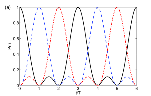
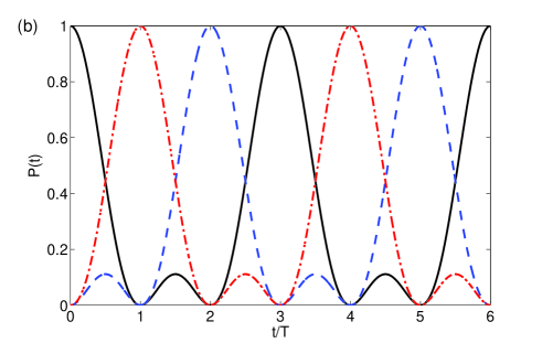
Figure 1: (Color online) The time evolution of the state occupation probabilities for the three-qubit system with $\phi_{ij}=\pi/2$. (a) One-excited case with initial state $|100\rangle$. The excitation from qubit $Q_{1}$ (black solid line) is swapped to qubit $Q_{2}$ (blue dash line) at time $T$ and then to qubit $Q_{3}$ (red dash dot line) at time $2T$, and then repeat this circle. (b) Two-excited case with initial state $|011\rangle$, the population of $|011\rangle$ (black solid line) transfer to $|110\rangle$ (red dash dot line) at time $T$ and then to $|101\rangle$ (blue dash line) at time $2T$, and then repeat this circle.

Now we consider the cases that inter-qubit coupling amplitudes are pure imaginary numbers, i.e., set $\phi_{ij}=\pi/2$. The Hamiltonian in Eq. (2) commutes with $\sum_{i}\sigma_{i}^{z}$ and the number of excitation is conserved. We first investigate the single-excitation dynamics in the subspace expanded by $|100\rangle$, $|010\rangle$ and $|001\rangle$, in which the Hamiltonian has the following matrix representation

$$M_{1}=\hbar\frac{g_{0}}{2}\left(\begin{array}[]{ccc}0&i&-i\\ -i&0&i\\ i&-i&0\end{array}\right).$$ (3)

The eigen frequencies are $\lambda_{1}=0$, $\lambda_{2}=\frac{\sqrt{3}}{2}g_{0}$ and $\lambda_{3}=-\frac{\sqrt{3}}{2}g_{0}$. The corresponding eigenstates are

$$|\psi_{1}\rangle=\frac{1}{\sqrt{3}}\left(|100\rangle+|010\rangle+|001\rangle\right),$$ (4)

$$|\psi_{2}\rangle=\frac{1}{\sqrt{3}}\left(|100\rangle+e^{i2\pi/3}|010\rangle+e^{i4\pi/3}|001\rangle\right),$$

$$|\psi_{3}\rangle=\frac{1}{\sqrt{3}}\left(|100\rangle+e^{i4\pi/3}|010\rangle+e^{i2\pi/3}|001\rangle\right).$$

If we initially prepare the state $|\Psi(0)\rangle=|100\rangle=\left(|\psi_{1}\rangle+|\psi_{2}\rangle+|\psi_{3}\rangle\right)/\sqrt{3}$, the evolution of the wavefunction is

$$|\Psi\left(t\right)\rangle= \frac{1}{\sqrt{3}}\sum\limits_{j=1}^{3}e^{-i\lambda_{j}t}|\psi_{j}\rangle$$ (5)

$$= \frac{1}{3}\left[\left(1+2\cos\left(\frac{\sqrt{3}}{2}g_{0}t\right)\right)|100\rangle\right.$$

$$+\left(1+2\cos\left(\frac{\sqrt{3}}{2}g_{0}t-2\pi/3\right)\right)|010\rangle$$

$$+\left.\left(1+2\cos\left(\frac{\sqrt{3}}{2}g_{0}t+2\pi/3\right)\right)|001\rangle\right].$$

It is clear that at time $t=T\equiv 4\pi/(3\sqrt{3}g_{0})$, $|\Psi\left(T\right)\rangle=|010\rangle$, and at time $t=2T$, $|\Psi\left(2T\right)\rangle=|001\rangle$, as shown in Fig.1 (a).

Next we consider the subspace containing two excitations, $|011\rangle$, $|101\rangle$ and $|110\rangle$, the reversed states of the three states in the single excitation subspace. The corresponding matrix of the Hamiltonian is

$$M_{2}=-M_{1}.$$ (6)

The overall minus sign indicates a excitation rotation in the opposite direction. The evolution of an initial state $|011\rangle$ can be obtained by changing $g_{0}$ to $-g_{0}$ and reversing the states in Eq. (5). The time evolution of the state occupation probabilities is plotted in Fig. 1 (b). For clearly see the difference of the time evolution of above two cases, we also plot a schematic figure for the single-excitation and two-excitation circulation, see Fig. 2 .

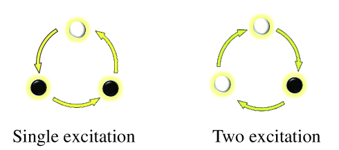
Figure 2: Excitation circulation for single- and two-excitation cases in three-qubit loop. The white dot stand for qubit in the excited state and the black dot stand for qubit in the ground state. While the single excitation rotate in the anticlockwise direction, the two excitations rotate in the reverse direction.

The surprising results that the single-excitation and two-excitation cases have different circulation directions can be understood as following. The state $|011\rangle\rightarrow|100\rangle$ can be seen as simply reverse the definition of $\left|0\right\rangle$ and $\left|1\right\rangle$. To express the Hamiltonian in this reversed new basis, we need to switch $\sigma_{j}^{+}\rightarrow\sigma_{j}^{-}$ and $\sigma_{j}^{-}\rightarrow\sigma_{j}^{+}$, which results in $H\rightarrow-H$. The state will evolve backward in time equivalently. Actually, the condition to produce this different circulations for single- and two-excitation cases, i.e., $\phi_{ij}=\pi/2$, can be loosen to $\Phi=\phi_{12}+\phi_{23}+\phi_{31}=\pm\pi/2$. The total phase $\Phi$ can be seen as an effective magnetic flux. The restrictive phase of oscillating coupling introduce a effective magnetic field, which produce the circulation of qubit excitation.

III protocol for generating ghz states

The directional circulation of excitation allow us to produce GHZ state by turning on the interaction for a definite duration and manipulating a sequence of electromagnetic pulses. Firstly, we prepare three-qubit GHZ state, and then extend it to produce large-number GHZ states. The devise employed here is a superconducting circuit lattice Circuit QED Lattices ; naturePhysics_Martinis . A schematic diagram is shown in Fig. 3. With mature nanofabrication techniques, the circuit QED can be assemble as design. The most important experimental technology for realizing our scheme is tunable coupling between qubits, which is reported in reference Martinis-PRL-2014 .

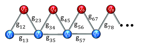
Figure 3: Schematic diagram of circuit QED lattice. The coupling between any two qubits is tunable $g_{ij}\left(t\right)=g_{0}\cos\left(\Delta_{ij}t+\phi_{ij}\right),$ with $\Delta_{ij}$ equal to the frequency difference between $Q_{i}$ and $Q_{j}$.The simplest operation for realizing our protocol is use $\omega_{1}=\omega_{3}=\omega_{5}=\omega_{7}\cdots,$ $\omega_{2}=\omega_{4}=\omega_{6}=\omega_{8}\cdots$, $\Delta_{13}=\Delta_{35}=\Delta_{57}=\cdots=0,$ $\Delta_{12}=\Delta_{23}=\Delta_{34}=\Delta_{45}=\cdots=\omega_{1}-\omega_{2},$ $\phi_{12}=\phi_{34}=\phi_{56}=\cdots=\pi/2$, and $\phi_{23}=\phi_{45}=\phi_{67}=\cdots=0$.

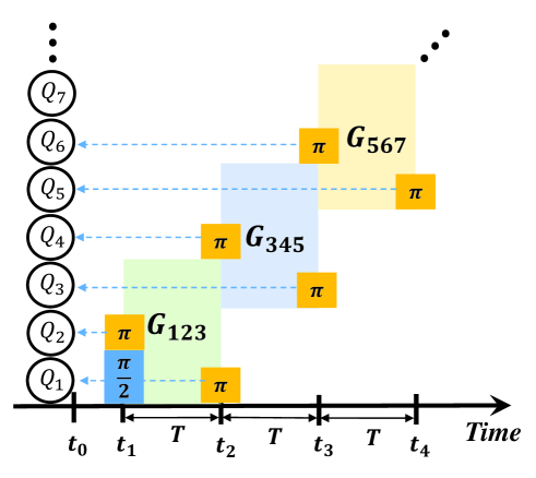
Figure 4: Sequence of operations. The blue box stand for a $\pi/2$ pulse and the yellow box stand for a $\pi$ pulse. They act on the qubits that arrows point to at the determinate points in time $t_{i}$. The characteristic time for excitation swapping is $T=4\pi/(3\sqrt{3}g_{0})$. The shaded area in color label with $G_{123}$($G_{345}$, $G_{567}$) mean turning on the couplings in the corresponding three-qubit loop.

time	states transfer under $\pi/2$ and $\pi$ pulse
$t_{1}$	$|0000000\cdots 0\rangle$$\rightarrow$$\frac{1}{\sqrt{2}}\left(|0\rangle+|1\rangle\right)_{1}\otimes|100000\cdots 0\rangle$
$t_{2}$	$\frac{1}{\sqrt{2}}\left(|100\rangle+|011\rangle\right)_{123}\otimes|0\cdots 00\rangle\rightarrow\frac{1}{\sqrt{2}}\left(|000\rangle+|111\rangle\right)_{123}\otimes|1\cdots 00\rangle$
$t_{3}$	$\frac{1}{\sqrt{2}}\left(|00100\rangle+|11011\rangle\right)_{12345}\otimes|0\cdots 00\rangle\rightarrow\frac{1}{\sqrt{2}}\left(|00000\rangle+|11111\rangle\right)_{12345}\otimes|1\cdots 00\rangle$
$t_{4}$	$\frac{1}{\sqrt{2}}\left(|0000100\rangle+|1111011\rangle\right)_{1234567}\otimes|0\cdots 00\rangle\rightarrow\frac{1}{\sqrt{2}}\left(|0000000\rangle+|1111111\rangle\right)_{1234567}\otimes|0\cdots 00\rangle$

Table 1: State evolution, basic steps of generation GHZ states. $t_{1}$: prepare the first qubits in a superposition of 0 and 1 state, flip the second qubits. $t_{1}\rightarrow t_{2}$: introduce an interaction $G_{123}$ among first three qubits, which leads to opposite rotations of the two states as shown in Eq.(7). $t_{2}$, send in $\pi$ pulse to flip the first and fourth qubits. $t_{2}\rightarrow t_{3}$: introduce the same interaction as in $t_{1}\rightarrow t_{2}$ with $G_{345}$. $t_{3}$, send in $\pi$ pulse to flip the third and sixth qubits. Repeat steps to realize GHZ state for larger number of qubits, each time adding two qubits to the GHZ chain. For a GHZ state with $2n+1$ qubits, we need in total $2n$ $\pi$ pulses and one $\pi/2$ pulse.

The sequence of operations is shown in Fig. 4. We start from ground state $|000\cdots 00\rangle$. At time $t_{1}$, we send a $\pi/2$ pulse to $Q_{1}$ and a $\pi$ pulse to $Q_{2}$. Qubit $Q_{1}$ is been prepared in a superposition state $\frac{1}{\sqrt{2}}\left(|0\rangle+|1\rangle\right)$ and $Q_{2}$ is been flipped to $|1\rangle$ state. The state of system transfer to $\frac{1}{\sqrt{2}}\left(|0\rangle+|1\rangle\right)_{1}\otimes|100\cdots 00\rangle$. The following step is crucial. We switch on the couplings among the first three qubits (denoted by $G_{123}$), as demonstrated in above section, the three-qubit loop undergo opposite rotations for $\left|010\right\rangle$ and $\left|110\right\rangle$ states.

$$|010\rangle\rightarrow|100\rangle\rightarrow|001\rangle\rightarrow|010\rangle,$$ (7)

$$|110\rangle\rightarrow|011\rangle\rightarrow|101\rangle\rightarrow|110\rangle.$$

After a definite time $T=4\pi/(3\sqrt{3}g_{0})$, turn off the interactions $G_{123}$, the system evolve to $\frac{1}{\sqrt{2}}\left(|100\rangle+|011\rangle\right)_{123}\otimes|0\cdots 00\rangle$ state. Then, we send a $\pi$ pulse to flip the first qubit. The first three qubits are in a GHZ state. Next we continue our production of multiqubit GHZ state: send a $\pi$ pulse to the fourth qubit and switch on the same special couplings among the third, fourth and fifth qubits (denoted by $G_{345}$). After these three-qubit states undergo the process $|010\rangle\rightarrow|100\rangle$ and $|110\rangle\rightarrow|011\rangle$ in Eq. (7) for the two component of the superposition state, respectively, we obtain the state $\frac{1}{\sqrt{2}}\left(|00100\rangle+|11011\rangle\right)_{12345}$. Then we send a $\pi$ pulse to the third qubit, the first five qubits are prepared in a 5-qubit GHZ state, as shown in Tab. 1. We can repeat the process to generate the GHZ state involving more qubits.

Above scheme is only for odd-number GHZ states. For even-number GHZ states, we can use same method base on two-qubit Bell state $\frac{1}{\sqrt{2}}\left(|00\rangle+|11\rangle\right)_{12}$. The entangled Bell states for superconducting qubit have been validly studied and realized in several experiments Bell-state1 ; Bell-state2 ; Bell-staet3 ; Bell-state4 . Starting in the ground state, a $\pi/2$ pulse is applied to qubit $Q_{1}$ to create the superposition $\frac{1}{\sqrt{2}}\left(|0\rangle+|1\rangle\right)_{1}\otimes|0\cdots 00\rangle$. Next, a CNOT gate is applied to flip qubit $Q_{2}$ conditioned on qubit $Q_{1}$, resulting in the Bell state $\frac{1}{\sqrt{2}}\left(|00\rangle+|11\rangle\right)_{12}\otimes|0\cdots 00\rangle$ three-GHZ2 ; Bell-state2 . Following the above described method, we can generate large even-number GHZ states.

IV preparation errors and fidelity

In this section, we analyze the experimental feasibility of our scheme by investigating preparation errors. Errors mainly come from two aspects. The first one is the precision of the control of the interaction time. For each “rotation” operation, if the interaction time is not exactly $T$, the state realized is not a exact GHZ state. The second is the environmental noises. We refer to recent experimental achievement to discuss the feasibility of our scheme. The operations of switching on (off) and dynamically modulating of inter-qubit coupling in circuit QED can be in nanosecond timescales Martinis-PRL-2014 . The typical qubit-qubit coupling strength is several megahertz naturePhysics_Martinis , so the characteristic time $T$ for excitation circulation is hundreds of nanosecond. The switching time is much less than $T$, therefore, the precision of the control of the interaction time made the error acceptable.

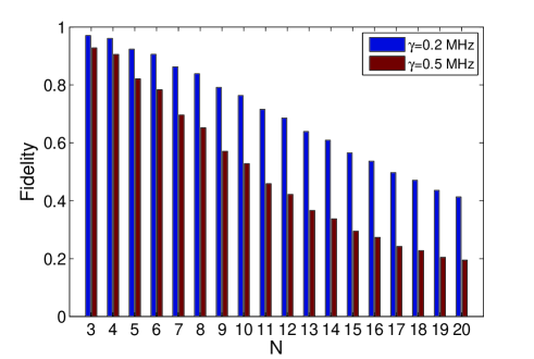
Figure 5: (Color online) Fidelity for different N-qubit GHZ states. Two kinds of bars corresponding to decay rate of qubit $\gamma=0.2\thinspace\mathrm{MHz}$ (blue bar) and $\gamma=0.5\thinspace\mathrm{MHz}$ (red bar). The characteristic time for excitation circulation $T=100\thinspace\mathrm{ns}$.

The qubit relaxation and dephasing during the operation certainly changes the final output state. In contrast to natural atoms, an advantage of superconducting qubit is that its coherence time can be large as tens of microseconds T1-1 ; T1-2 ; T1-3 . We calculate the fidelity for N-qubit GHZ state in our scheme. To be on the safe said, we assume for the qubit $T=100\thinspace\mathbf{\mathrm{ns}}$, and choose two decay rates $\gamma=0.2\thinspace\mathrm{MHz}$ and $\gamma=0.5\thinspace\mathrm{MHz}$ for reference. The results are shown in Fig. 5, where for even-number GHZ state, we neglect the errors in preparing initial Bell state.

Definitely, there will be other complicated factors influencing the fidelity of GHZ state in real preparation process. Here, our analysis is optimistic but the parameter we chosen for qubit decay rate is not rigorous compare to existing experiments. In the Ref. naturePhysics_Martinis , a similar circulation of photons can exist several cycles in the coherence time of superconducting qubit. Therefore, we have confidence that our scheme can work in appropriate circuit QED system.

V conclusion

In conclusion, we propose a totally new mechanism for generation of multiqubit GHZ states. The essential of this scheme is the directional excitation circulation in three-qubit coupling loop, and this phenomenon is derived from the complex hopping amplitude which break the time-reversal symmetry. We can realize the pure imaginary hopping constant by dynamically modulating the inter-qubit coupling which has been realized in circuit QED experiment. There is another method to obtain the effective interaction with imaginary hopping amplitude by dynamically modulating the frequency of qubit Dawei2016PRL . Based on these modulating methods, our scheme for generation of multiqubit GHZ state can be applied to other system. In this paper, we employ superconducting qubit to demonstrate the experimental feasibility of our scheme. Our results of fidelity analysis show the scheme is realizable with the existing experimental conditions.

- (1) A. Einstein, B. Podolsky, and N. Rosen, Can quantummechanical description of physical reality be considered complete?, Phys. Rev. 47, 777 (1935).
- (2) John S. Bell, On the Einstein Podolsky Rosen paradox, Physics 1, 195 (1964).
- (3) J. W. Pan, D. Bouwmeester, M. Daniell, H. Weinfurter, A. Zeilinger, Nature (London) 403, 515 (2000).
- (4) J. Handsteiner et al., Cosmic Bell Test: Measurement Settings from Milky Way Stars, Phys. Rev. Lett. 118, 060401 (2017).
- (5) M. A. Nielsen, I. L. Chuang, Quantum Computation and Quantum Information (Cambridge University Press, Cambridge, 2000).
- (6) I. M. Georgescu, S. Ashhab, and Franco Nori, Quantum simulation, Rev. Mod. Phys. 86, 153 (2014).
- (7) V. Giovannetti, S. Lloyd, and L. Maccone, Quantum-Enhanced Measurements: Beating the Standard Quantum Limit, Science 306, 1330 (2004).
- (8) D. M. Greenberger, M. A. Horne, A. Shimony, and A. Zeilinger, Bell’s theorem without inequalities, Am. J. Phys. 58, 1131 (1990).
- (9) M. Hillery, V. Buzek, and A. Berthiaume, Phys. Rev. A 59, 1829 (1999).
- (10) A. Zeilinger, M. A. Horne, H. Weinfurter, and M. Żukowski, Three-Particle Entanglements from Two Entangled Pairs, Phys. Rev. Lett. 78, 3031 (1997).
- (11) D. Bouwmeester, Jian-Wei Pan, M. Daniell, H. Weinfurter, and A. Zeilinger, Phys. Rev. Lett. 82, 1345 (1999).
- (12) L. K. Chen, Z. D. Li, X. C. Yao, M. Huang, W. Li, H. Lu, X. Yuan, Y. B. Zhang, X. Jiang, C. Z. Peng, L. Li, N. L. Liu, X. Ma, C. Y. Lu, Y. A. Chen, and J. W. Pan, Optica 4, 77 (2017).
- (13) S. B. Zheng, Phys. Rev. Lett. 87, 230404 (2001).
- (14) K. Mølmer and A. Sørensen, Multiparticle Entanglement of Hot Trapped Ions, Phys. Rev. Lett. 82, 1835 (1999).
- (15) T. Monz, P. Schindler, J. T. Barreiro, M. Chwalla, D. Nigg, W. A. Coish, M. Harlander, W. Hansel, M. Hen- nrich, and R. Blatt, 14-Qubit Entanglement: Creation and Coherence, Phys. Rev. Lett. 106, 130506 (2011).
- (16) K. Helmerson and L. You, Phys. Rev. Lett. 87, 170402 (2001).
- (17) L. You, Phys. Rev. Lett. 90, 030402 (2003).
- (18) P. Neumann, N. Mizuochi, F. Rempp, P. Hemmer, H. Watanabe, S. Yamasaki, V. Jacques, T. Gaebel, F. Jelezko, J. Wrachtrup, Science. 320, 1326 (2008).
- (19) X. W. Xu, Y. J. Zhao, and Y. X. Liu, Phys. Rev. A 88, 022325 (2013).
- (20) J. Q. You and F. Nori, Nature (London) 474, 589 (2011).
- (21) Y. Makhlin, G. Schon, and A. Shnirman, Rev. Mod. Phys. 73, 357 (2001).
- (22) J. Clarke and F. K.Wilhelm, Nature (London) 453, 1031 (2008).
- (23) J. E. Mooij, T. P. Orlando, L. Levitov, L. Tian, C. H. van der Wal, and S. Lloyd, Science 285, 1036 (1999).
- (24) W. Feng, Y. Li, and S. Y. Zhu, Phys. Rev. A, 89, 013816 (2014).
- (25) M. Hofheinz et al., Nature (London) 459, 546 (2009).
- (26) Y. Chen, C. Neill, P. Roushan, N. Leung, M. Fang, R. Barends, J. Kelly, B. Campbell, Z. Chen, B. Chiaro, A. Dunsworth, E. Jeffrey, A. Megrant, J. Y. Mutus, P. J. J. O’Malley, C. M. Quintana, D. Sank, A. Vainsencher, J. Wenner, T. C. White, M. R. Geller, A. N. Cleland, and J. M. Martinis, Qubit Architecture with High Coherence and Fast Tunable Coupling, Phys. Rev. Lett. 113, 220502 (2014).
- (27) S. Schmidt and J. Koch, Circuit QED Lattices: Towards Quantum Simulation with Superconducting Circuits, Ann. Phys. (Amsterdam) 525, 395 (2013).
- (28) Y. D. Wang, S. Chesi, D. Loss, and C. Bruder, Phys. Rev. B 81, 104524 (2010).
- (29) S. Aldana, Y. D. Wang, and C. Bruder, Phys. Rev. B 84, 134519 (2011).
- (30) L. F. Wei, Y. X. Liu, and F. Nori, Phys. Rev. Lett. 96, 246803 (2006).
- (31) F. Helmer and F. Marquardt, Phys. Rev. A 79, 052328 (2009).
- (32) A. Galiautdinov, M. W. Coffey, and R. Deiotte, Phys.Rev.A 80, 062302 (2009).
- (33) W. Feng, P. Wang, X. Ding, L. Xu, and X. Q. Li, Phys.Rev.A 83, 042313 (2011).
- (34) D. I. Tsomokos, S. Ashhab, and F. Nori, New J. Phys. 10, 113020 (2008).
- (35) L. S. Bishop, L. Tornberg, D. Price, E. Ginossar, A. Nunnenkamp, A. A. Houck, J. M. Gambetta, J. Koch, G. Johansson, S. M. Girvin, New J. Phys. 11, 073040 (2009).
- (36) L. DiCarlo, M. D. Reed, L. Sun, B. R. Johnson, J. M. Chow, J. M. Gambetta, L. Frunzio, S. M. Girvin, M. H. Devoret, and R. J. Schoelkopf, Nature (London) 467, 574 (2010).
- (37) M. Neeley, R. C. Bialczak, M. Lenander, E. Lucero, M. Mariantoni, A. D. O’Connell, D. Sank, H. Wang, M. Weides, J. Wenner, Y. Yin, T. Yamamoto, A. N. Cleland, and J. M. Martinis, Nature (London) 467, 570 (2010).
- (38) R. Barends, J. Kelly, A. Megrant, A. Veitia, D. Sank, E. Jeffrey, T. C. White, J. Mutus, A. G. Fowler, B. Campbell, Y. Chen, Z. Chen, B. Chiaro, A. Dunsworth, C. Neill, P. O’Malley, P. Roushan, A. Vainsencher, J. Wenner, A. N. Korotkov, A. N. Cleland, and John M. Martinis, Nature 508, 500 (2014).
- (39) P. Roushan, et al., Chiral ground-state currents of interacting photons in a synthetic magnetic field, Nature Physics, 13, 146 (2017).
- (40) M. Steffen, M. Ansmann, R. C. Bialczak, N. Katz, E. Lucero, R. McDermott, M. Neeley, E. M. Weig, A. N. Cleland, and J. M. Martinis, Science 313, 1423 (2006).
- (41) J. H. Plantenberg, P. C. de Groot, C. J. P. M. Harmans, and J. E. Mooij, Nature (London) 447, 836 (2007).
- (42) L. DiCarlo, J. M. Chow, J. M. Gambetta, L. S. Bishop, B. R. Johnson, D. I. Schuster, J. Majer, A. Blais, L. Frunzio, S. M. Girvin, and R. J. Schoelkopf, Nature (London) 460, 240 (2009).
- (43) M. Ansmann, H. Wang, R. C. Bialczak, M. Hofheinz, E. Lucero, M. Neeley, A. D. O’Connell, D. Sank, M. Weides, J. Wenner, A. N. Cleland, and J. M. Martinis, Nature (London) 461, 504 (2009).
- (44) R. Barends, J. Kelly, A. Megrant, D. Sank, E. Jeffrey, Y. Chen, Y. Yin, B. Chiaro, J. Mutus, C. Neill, P. O’Malley, P. Roushan, J. Wenner, T. C. White, A. N. Cleland, and J. M. Martinis, Phys. Rev. Lett. 111, 080502 (2013).
- (45) Chad Rigetti, Jay M. Gambetta, Stefano Poletto, B. L. T. Plourde, Jerry M. Chow, A. D. Córcoles, John A. Smolin, Seth T. Merkel, J. R. Rozen, George A. Keefe, Mary B. Rothwell, Mark B. Ketchen, and M. Steffen, Phys. Rev. B 86, 100506(R) (2012).
- (46) Hanhee Paik, D. I. Schuster, Lev S. Bishop, G. Kirchmair, G. Catelani, A. P. Sears, B. R. Johnson, M. J. Reagor, L. Frunzio, L. I. Glazman, S. M. Girvin, M. H. Devoret, and R. J. Schoelkopf, Phys. Rev. Lett. 107, 240501 (2011).
- (47) D. W. Wang, H. Cai, R. B. Liu, and M. O. Scully, Mesoscopic Superposition States Generated by Synthetic Spin-Orbit Interaction in Fock-State Lattices, Phys. Rev. Lett. 116, 220502 (2016).