A study of jet mass distributions with grooming

Abstract

We perform a phenomenological study of the invariant mass distribution of hadronic jets produced in proton-proton collisions, in conjunction with a grooming algorithm. In particular, we consider the modified MassDrop Tagger (mMDT), which corresponds to Soft Drop with angular exponent $\beta=0$. Our calculation, which is differential in both jet mass and jet transverse momentum, resums large logarithms of the jet mass, including the full dependence on the groomer’s energy threshold $z_{\text{cut}}$, and it is matched to fixed-order QCD matrix elements at next-to-leading order. In order to account for non-perturbative contributions, originating from the hadronisation process and from the underlying event, we also include a phenomenological correction factor derived from Monte Carlo parton shower simulations. Furthermore, we consider two different possibilities for the jet transverse momentum: before or after grooming. We show that the former should be preferred for comparisons with upcoming experimental data essentially because the mMDT transverse momentum spectrum is not collinear safe, though the latter exhibits less sensitivity to underlying event and displays properties that may provide complementary information for probing non-perturbative effects.

1 Introduction

The CERN Large Hadron Collider has been running at an energy of 13 TeV in the centre-of-mass frame, thus reaching energies far above the electroweak scale. Consequently, $Z/W^{\pm}$, Higgs, top quarks and any new particle with a mass around the electroweak scale can be produced with a large boost, causing their hadronic decays to become collimated so that they may be reconstructed as a single jet Seymour:1993mx ; Butterworth:2002tt . As a results, jet substructure is playing a central role during Run-II of the LHC and its importance is only going to increase for future runs, as well as at future higher-energy colliders Abdesselam:2010pt ; Altheimer:2012mn ; Altheimer:2013yza ; Adams:2015hiv . For example, even though not confirmed in Run-II (see e.g. ATLAS:2016yqq ), an interesting excess in the invariant mass distribution of two $W$ bosons was observed with Run-I data Aad:2015owa ; Khachatryan:2014hpa , relying on jet-substructure techniques to isolate the signal from the QCD background.

Jet substructure studies aim to better understand radiation patterns in jets, in order to build efficient algorithms that can distinguish signal jets from the QCD background. Examples include jet angularities Berger:2003iw ; Ellis:2010rwa , energy-energy correlation functions Larkoski:2013eya ; Moult:2016cvt , and other jet shapes Seymour:1997kj ; Thaler:2010tr ; Thaler:2011gf ; Salam:2016yht ; Dasgupta:2016ktv ; Larkoski:2015kga ; Larkoski:2014gra ; Larkoski:2014zma of high-$p_{t}$ jets. Perhaps the simplest example of such observables is the jet invariant mass. Signal jets, which originate from the decay of a boosted massive particle, are expected to have a mass in the region of that massive state. QCD jets instead acquire mass through parton branching and their mass is proportional to the jet transverse momentum. Thus, a cut on the jet mass could be, in principle, a good discriminant. However, many issues come into play and make this simple picture too naive. First, the mass of QCD jets often appears to be in the same range as the signal jets. Then, radiation can leak outside the jet, altering both signal and background. Moreover, hadron colliders are not clean environments and there are many sources of additional, non-perturbative, radiation that pollute the parton-level picture, e.g. the underlying event, caused by secondary scattering in a proton-proton collision, and pile-up, caused by multiple proton-proton interactions.

For the above reasons, many substructure algorithms, often referred to as “groomers” and “taggers”, have been developed. Broadly speaking, a grooming procedure takes a jet as an input and tries to clean it up by removing constituents which, being at wide angle and relatively soft, are likely to come from contamination, such as the underlying event or pile-up. A tagging procedure instead focuses on some kinematic variable that is able to distinguish signal from background, such as, for instance, the energy sharing between two prongs within the jet, and cuts on it. Many of the most commonly used substructure algorithms such as the MassDrop Tagger (MDT) Butterworth:2008iy , trimming Krohn:2009th , pruning Ellis:2009su ; Ellis:2009me , or Soft Drop Larkoski:2014wba perform both grooming and tagging, so a clear distinction between the two is not always obvious. These techniques have now been successfully tested and are currently used in experimental analyses.

A quantitative understanding of groomed jet cross sections and distributions is of paramount importance not only in order to devise more efficient substructure algorithms but also in order to understand their systematics, thus assessing their robustness. For instance, the study of Refs. Dasgupta:2013ihk ; Dasgupta:2013via revealed unwanted features (kinks) in the mass distribution of background jets with certain grooming algorithms, such as trimming and pruning, that deteriorate the discrimination power at high $p_{t}$. Therefore, more robust grooming techniques, with better theoretical properties, such as the modified MassDrop Tagger (mMDT) Dasgupta:2013ihk and Soft Drop Larkoski:2014wba , defined in Section 2, were developed in order to overcome these issues. A deeper understanding of these tools can be achieved by comparing accurate theoretical predictions to data. On the experimental side, one would like to have unfolded distributions of substructure variables measured on QCD jets, as for instance in Refs. ATLAS:2012am ; Chatrchyan:2013vbb . On the theory side, all-order calculations have been performed for a variety of substructure variables with Soft Drop (or mMDT) Larkoski:2014wba , such as the jet invariant mass, energy correlations, the effective groomed radius and the prongs’ momentum sharing Larkoski:2015lea . More recently, using the framework of Soft-Collinear Effective Theory (SCET), these calculations have achieved the precision frontier, reaching next-to-next-to-leading logarithmic accuracy (NNLL) Frye:2016okc ; Frye:2016aiz , albeit in some approximation, such as the small-$z_{\text{cut}}$ limit, as we will discuss in what follows. Furthermore, it has been shown that jet observables with grooming are less sensitive to non-perturbative corrections than traditional ones. This was expected in the case of contamination from the underlying event and pile-up because groomers are indeed designed to remove soft radiation at large angle, which constitutes the bulk of these contributions. Less obvious, but now understood from a variety of Monte Carlo simulations as well as theoretical considerations, is the reduction of the hadronisation contribution. These properties contribute to make groomed distribution even more amenable for comparisons between data and calculations in perturbative QCD.

In this paper, we perform a phenomenological study of the jet mass distribution with mMDT — also corresponding to Soft Drop with $\beta=0$ — motivated by an upcoming CMS measurement CMS-coming . We consider jet mass distributions in several transverse momentum bins. Our theoretical prediction accounts for the resummation of the leading large logarithms of the ratio of the jet mass over the jet transverse momentum and it is matched to fixed-order matrix elements computed at next-to-leading order (NLO). While the accuracy of this resummation is one logarithmic order less than the one presented in Refs. Frye:2016okc ; Frye:2016aiz in the case $\beta=0$, we do lift the small-$z_{\text{cut}}$ approximation. Crucially, working at finite $z_{\text{cut}}$ allows us to keep track of the distinction between the jet transverse momentum before or after grooming, henceforth $p_{t,\text{jet}}$ and $p_{t,\text{\text{mMDT}}}$, respectively. The two are, of course, equal at $z_{\text{cut}}=0$. We find that the use of $p_{t,\text{\text{mMDT}}}$ has several theoretical disadvantages with respect to $p_{t,\text{jet}}$. While the two resummations coincide as $z_{\text{cut}}\to 0$, the $p_{t,\text{\text{mMDT}}}$ selection leads to a more involved perturbative structure even at the leading nontrivial order. This difference stems from a basic fact, namely while the ungroomed $p_{t,\text{jet}}$ spectrum is an Infra-Red and Collinear (IRC) safe quantity, the jet $p_{t,\text{\text{mMDT}}}$ spectrum (with no additional cuts) is Sudakov safe Larkoski:2013paa ; Larkoski:2014wba ; Larkoski:2015lea but not IRC safe. Conversely, the $p_{t,\text{\text{mMDT}}}$ spectrum is less sensitive to the underlying event than $p_{t,\text{jet}}$ one and, arguably, more resilient to pile-up. It is therefore interesting to explore both options in more details.

This paper is organised as follows. In Section 2 we review definition and properties of Soft Drop and mMDT. Resummation and matching of the mass distribution with $p_{t,\text{jet}}$ are done in Section 3, followed by the case of $p_{t,\text{\text{mMDT}}}$ in Section 4. A Monte Carlo study of non-perturbative corrections is presented in Section 5, while we collect our final phenomenological predictions in Section 6. Finally, we conclude in Section 7.

2 A brief reminder of the grooming procedure

The Soft Drop grooming procedure Larkoski:2014wba takes a jet with momentum $p_{t,\text{jet}}$ and radius $R$. It re-clusters its constituents using the Cambridge/Aachen (C/A) algorithm Dokshitzer:1997in ; Wobisch:1998wt and iteratively performs the following steps:

1. it de-clusters the jet into 2 subjets $j\to j_{1}+j_{2}$;

2. it checks the condition

   $$\frac{\min(p_{t1},p_{t2})}{p_{t1}+p_{t2}}>z_{\mathrm{cut}}\left(\frac{\theta_{12}}{R}\right)^{\beta}\,;$$ (1)

3. if the jet passes the condition, the recursion stops; if not the softer subjet is removed and the algorithms goes back to step 1 with the hardest of the two subjets.

As previously anticipated, in this study we only consider $\beta=0$. In this case Soft Drop essentially reduces to the mMDT, albeit without any actual mass-drop condition. Moreover, while the original MDT algorithm imposed a cut on the ratio of angular distances to masses, a so-called $y_{\mathrm{cut}}$, the mMDT variant instead cuts on momentum fractions Dasgupta:2013ihk (see e.g. Dasgupta:2013ihk ; Dasgupta:2016ktv for a comparison between $y_{\mathrm{cut}}$ and $z_{\mathrm{cut}}$).

From a theoretical point of view, Soft Drop has numerous advantages. For instance, non-global logarithms Dasgupta:2001sh ; Dasgupta:2002bw , which require sophisticated treatments, e.g. Banfi:2002hw ; Forshaw:2006fk ; Forshaw:2008cq ; DuranDelgado:2011tp ; Weigert:2003mm ; Hatta:2013iba ; Schwartz:2014wha ; Larkoski:2015zka ; Larkoski:2016zzc ; Neill:2016stq ; Caron-Huot:2015bja ; Becher:2015hka ; Becher:2016mmh and are often the bottle-neck of resummed calculations, are removed. Moreover, if we concentrate on mMDT, as we do here, the perturbative behaviour of observables such as the jet mass, which are double-logarithmic when measured on ungroomed jets, is changed into a single-logarithmic one because the soft-collinear region of phase-space is groomed away. Furthermore, the action of the groomer greatly reduces the impact of non-perturbative contributions, such as hadronisation, the underlying event and pile-up, extending the regime of validity of perturbation theory down to smaller values of the observables of interest. This opens up the possibility of performing sensible comparisons between data and first-principle theoretical predictions across a significant region of phase-space.

3 Jet mass distributions with mMDT

Throughout this paper, we focus on the invariant mass of a mMDT jet produced in proton-proton collisions with a centre-of-mass energy of 13 TeV. Our selection cuts closely follow the ones of the upcoming CMS measurement CMS-coming : jets are defined with the anti-$k_{t}$ algorithm Cacciari:2008gp with jet radius $R=0.8$. Next, we select the two hardest jets, $j_{a}$ and $j_{b}$, of the event and impose the following conditions:

1. both jets must have $p_{t,\text{jet}}>200\,\mathrm{GeV}$ and central rapidity, namely $|y|<2.4$;

2. the transverse momenta of the jets must satisfy $|p_{ta}-p_{tb}|<0.3(p_{ta}+p_{tb})$, in order to select symmetric configurations;

3. the jets should be well-separated in azimuth, i.e. $\Delta\phi_{j_{a},j_{b}}>\pi/2$.

In practice, these cuts are intended to select dijet events. We note however that the transverse momentum cut on the second jet results in large perturbative corrections for the dijet cross-section which render the mass distribution unstable in the first transverse momentum bin. Imposing only a $p_{t}$ cut on the leading jet and the symmetry condition would have been similarly efficient at selecting dijet events, and would have improved the perturbative convergence.

For every jet that passes the above cuts, we apply the mMDT procedure with $z_{\mathrm{cut}}=0.1$. We compute the (groomed) jet mass squared defined as $m^{2}=\left(\sum_{i}p_{i}\right)^{2},$ where the sum runs over all particles in the groomed jet. We also find useful to define the dimensionless variable

$$\rho=\frac{m^{2}}{p_{t,\text{jet}}^{2}R^{2}}.$$ (2)

We calculate the $\rho$ distribution in a given transverse momentum bin $p_{t1}<p_{t,\text{jet}}<p_{t2}$:

$$\frac{d\sigma}{d\rho}\left(\rho;z_{\mathrm{cut}},p_{t1},p_{t2}\right)=\int_{p_{t1}}^{p_{t2}}dp_{t,\text{jet}}\frac{d^{2}\sigma}{dp_{t,\text{jet}}d\rho}.$$ (3)

We also define the normalised distribution as

$$\frac{d\tilde{\sigma}}{d\rho}\left(\rho;z_{\mathrm{cut}},p_{t1},p_{t2}\right)=\frac{1}{\sigma_{\text{bin}}(p_{t1},p_{t2})}\frac{d\sigma}{d\rho}\left(\rho;z_{\mathrm{cut}},p_{t1},p_{t2}\right),$$ (4)

where $\sigma_{\text{bin}}$ is the jet cross section in the transverse momentum bin under consideration. We also explicitly consider the jet mass distribution

$$\frac{d\sigma}{dm}\left(m;z_{\mathrm{cut}},p_{t1},p_{t2}\right)=\int_{p_{t1}}^{p_{t2}}dp_{t,\text{jet}}\frac{d^{2}\sigma}{dp_{t,\text{jet}}dm}=\int_{p_{t1}}^{p_{t2}}dp_{t,\text{jet}}\frac{2m}{p_{t,\text{jet}}^{2}R^{2}}\frac{d^{2}\sigma}{dp_{t,\text{jet}}d\rho},$$ (5)

and the corresponding normalised version. Furthermore, the quantity that is measured experimentally is the mass distribution integrated over a set of mass bins $m_{i}<m<m_{i+1}$, which is the observable we are going to explicitly show in our plots. Note that in both Eq. (2) and Eq. (3) $p_{t,\text{jet}}$ is the jet transverse momentum before grooming. We will consider the alternative choice, namely the groomed transverse momentum $p_{t,\text{\text{mMDT}}}$ in Section 4.

Analytic all-order calculations of jet shapes with grooming is a rapidly developing field. In particular, the leading logarithmic resummation of mMDT jet masses has been performed in Dasgupta:2013ihk and resummation for Soft Drop observables, i.e. for generic $\beta$, was performed to NLL accuracy in Larkoski:2014wba and to NNLL accuracy in Frye:2016okc ; Frye:2016aiz . All the logarithmic contributions in Soft Drop observables are of collinear origin, while soft-emission at large angle can at most contribute with logarithms of $z_{\mathrm{cut}}$. Thanks to this observation, the resummed calculation can be done in the collinear limit and the resulting structure is much simpler than the one that we encounter in the resummation of the jet mass distributions without grooming, see for instance Dasgupta:2012hg ; Jouttenus:2013hs ; Chien:2012ur . In particular, soft radiation at large angle, which would give rise to a nontrivial matrix structure in colour space, is groomed away: only dipoles involving the measured jet are logarithmically enhanced and require resummation, while initial-state radiation does not contribute. For the same reason, these observables are free of non-global logarithms.

At this stage, a word of caution about our counting of the logarithmic accuracy is in order. While for a generic (non-zero) $\beta$, the Soft Drop mass distribution is dominated by double logarithms — with LL accuracy resumming those double logarithms, NLL accuracy including single-logarithms as well, etc… — these double logarithms are absent for mMDT (i.e. Soft Drop with $\beta=0$) in the region $\rho<z_{\mathrm{cut}}$:

$$\rho\frac{d\tilde{\sigma}}{d\rho}\left(\rho;z_{\mathrm{cut}}\right)=\left[\sum_{n=1}^{\infty}\sum_{m=1}^{n}c_{n,m}(z_{\mathrm{cut}})\,\alpha_{s}^{n}\log^{m-1}\left(\frac{1}{\rho}\right)+\mathcal{O}(\rho)\right],$$ (6)

where the dependence on the transverse momentum bin is understood. Single logarithmic terms in the jet mass are therefore formally the leading contribution and will be referred to as LL in what follows. The logarithmic counting of Refs. Frye:2016okc ; Frye:2016aiz differs from ours because it refers to the accuracy of the objects that appear in the factorisation theorem. These functions are separately double-logarithmic, even for $\beta=0$, and the cancellation of the double logarithms only happens when they are combined. In our counting, the NLL Larkoski:2014wba and NNLL Frye:2016okc ; Frye:2016aiz results obtained for a generic $\beta$, actually correspond respectively to LL and NLL accuracy, in the small $z_{\mathrm{cut}}$ limit, for mMDT. Thus, the state-of-the art evaluation of Eq. (6) accounts for all the coefficients $\tilde{c}_{n,n}(z_{\mathrm{cut}})$ and $\tilde{c}_{n,n-1}(z_{\mathrm{cut}})$, where

$$\lim_{z_{\mathrm{cut}}\to 0}c_{n,m}(z_{\mathrm{cut}})=\tilde{c}_{n,m}(z_{\mathrm{cut}})+\mathcal{O}(z_{\mathrm{cut}}).$$ (7)

For phenomenology, one typically uses $z_{\mathrm{cut}}\simeq 0.1$, so it is important to investigate the size of finite $z_{\mathrm{cut}}$ corrections. In this study we restrict ourselves to LL accuracy, while maintaining for the full $z_{\mathrm{cut}}$ dependence, i.e. we fully account for all coefficients $c_{n,n}(z_{\mathrm{cut}})$.

Finally, in the region $\rho>z_{\mathrm{cut}}$ grooming is not active and we recover the traditional jet mass result Dasgupta:2013ihk . In this region we are going to perform a less sophisticated calculation which resums the double logarithms and those single logarithmic contributions of collinear origin. We find this procedure acceptable because in this region $\rho\sim z_{\mathrm{cut}}$ and we expect these contributions to be less important than the fixed-order corrections, which we include at NLO.

3.1 Resummation at finite $z_{\mathrm{cut}}$

The resummation of the mMDT mass distribution at finite $z_{\mathrm{cut}}$ was outlined in Ref. Dasgupta:2013ihk in the fixed-coupling limit. The major complication with respect to the small-$z_{\mathrm{cut}}$ limit has to do with the flavour structure. Let us consider for instance a $q\to qg$ splitting which does not satisfy the mMDT condition. There is an $\mathcal{O}(z_{\mathrm{cut}})$ probability for the gluon to be harder than the quark. In such a case, the declustering sequence would follow the gluon branch rather than the quark, resulting into a nontrivial mixing between quarks and gluons. The resummed distribution therefore acquires a matrix structure in flavour space Dasgupta:2013ihk

$$\rho\dfrac{d^{2}\sigma}{dp_{t,\text{jet}}d\rho}=(R^{\prime}_{q}\;\;R^{\prime}_{g})\exp\left(\begin{array}[]{cc}-R_{q}-R_{q\to g}&R_{g\to q}\\ R_{q\to g}&-R_{g}-R_{g\to q}\end{array}\right)\left(\begin{array}[]{c}\sigma_{q}\\ \sigma_{g}\end{array}\right),$$ (8)

where $\sigma_{q(g)}$ is Born-level cross section for a quark (gluon) with transverse momentum $p_{t,\text{jet}}$ and $R^{\prime}_{q(g)}=\partial_{L}R_{q(g)}$, with $L=\log(1/\rho)$. As previously discussed, because we are dealing with a Soft Drop observable, the radiators $R_{i}$ can be computed in the collinear limit. Denoting by $\theta$ the emission angle (in units of the jet radius $R$) with respect to the hard momentum and with $z$ the momentum fraction, we have 

$$R_{q} =C_{F}\int_{0}^{1}\dfrac{d\theta^{2}}{\theta^{2}}\int_{0}^{1}dz\;p_{gq}(z)\dfrac{\alpha_{s}(z\theta p_{t,\text{jet}}R)}{\pi}\Theta\left(z_{\mathrm{cut}}<z<1-z_{\mathrm{cut}}\right)\Theta(z\theta^{2}>\rho),$$ (9a)

$$R_{g} =C_{A}\int_{0}^{1}\dfrac{d\theta^{2}}{\theta^{2}}\int_{0}^{1}dz\;p_{xg}(z)\dfrac{\alpha_{s}(z\theta p_{t,\text{jet}}R)}{\pi}\Theta\left(z_{\mathrm{cut}}<z<1-z_{\mathrm{cut}}\right)\Theta(z\theta^{2}>\rho),$$ (9b)

$$R_{q\to g} \>=\>C_{F}\int_{0}^{1}\dfrac{d\theta^{2}}{\theta^{2}}\int_{0}^{1}dz\;p_{gq}(z)\dfrac{\alpha_{s}(z\theta p_{t,\text{jet}}R)}{\pi}\Theta\left(1-z<z_{\mathrm{cut}}\right)\Theta(z\theta^{2}>\rho),$$ (9c)

$$R_{g\to q} =T_{R}n_{f}\int_{0}^{1}\dfrac{d\theta^{2}}{\theta^{2}}\int_{0}^{1}dz\;p_{qg}(z)\dfrac{\alpha_{s}(z\theta p_{t,\text{jet}}R)}{\pi}\left[\Theta\left(1-z<z_{\mathrm{cut}}\right)+\Theta\left(z<z_{\mathrm{cut}}\right)\right]\Theta(z\theta^{2}>\rho),$$ (9d)

where $C_{A}=3$, $C_{F}=4/3$, $T_{R}=1/2$, $n_{f}$ is the number of active quark flavours and $p_{ab}(z)$ are the splitting functions given in Appendix A.1.

At the LL accuracy we are working at, the above expressions can be further simplified. Besides the strict leading-logarithmic terms in $\rho$, it is trivial to also include the double-logarithmic terms in $z_{\mathrm{cut}}$ and this allows for a more transparent treatment of the transition point at $\rho=z_{\mathrm{cut}}$. In that context, it is helpful to separate Eq. (9) in a contribution $\mathcal{R}_{i}$, coming from the $1/z$ part of the splitting function that includes the logarithmic and constant terms in $z_{\mathrm{cut}}$, and a remainder which contains the corrections power-suppressed in $z_{\mathrm{cut}}$. Later, this will make it easy to study the size of the finite-$z_{\mathrm{cut}}$ corrections. For these contributions, we neglect the $z$ factor in the argument of $\alpha_{s}$ and in the constraint $z\theta^{2}>\rho$. The details of our calculation are given in Appendix A.1 and, our final result reads

$$R_{q} =C_{F}\mathcal{R}_{q}(\rho;z_{\mathrm{cut}})\,\Theta(\rho<e^{B_{q}})+C_{F}\,\mathcal{I}(\rho;z_{\mathrm{cut}})\,\pi_{q}(z_{\mathrm{cut}})\,\Theta(\rho<z_{\mathrm{cut}}),$$ (10a)

$$R_{g} =C_{A}\mathcal{R}_{g}(\rho;z_{\mathrm{cut}})\,\Theta(\rho<e^{B_{g}})+C_{A}\,\mathcal{I}(\rho;z_{\mathrm{cut}})\,\pi_{g}(z_{\mathrm{cut}})\,\Theta(\rho<z_{\mathrm{cut}}),$$ (10b)

$$R_{q\to g} =C_{F}\,\mathcal{I}(\rho;z_{\mathrm{cut}})\,\pi_{q\to g}(z_{\mathrm{cut}})\,\Theta(\rho<z_{\mathrm{cut}}),$$ (10c)

$$R_{q\to g} =n_{f}T_{R}\,\mathcal{I}(\rho;z_{\mathrm{cut}})\,\pi_{g\to q}(z_{\mathrm{cut}})\,\Theta(\rho<z_{\mathrm{cut}}),$$ (10d)

where we have introduced

$$\mathcal{R}_{i}(\rho;z_{\mathrm{cut}}) =\frac{1}{2\pi\alpha_{s}\beta_{0}^{2}}\Big{[}W\big{(}1+2\alpha_{s}\beta_{0}B_{i}\big{)}-W\big{(}1+2\alpha_{s}\beta_{0}\log(z_{m})\big{)}$$ (11a)

$$\phantom{=\frac{1}{2\pi\alpha_{s}\beta_{0}^{2}}}+2W\big{(}1+\alpha_{s}\beta_{0}\log(\rho z_{m})\big{)}-2W\big{(}1+\alpha_{s}\beta_{0}(\log(\rho)+B_{i})\big{)}\Big{]},$$

$$\mathcal{I}(\rho;z_{\mathrm{cut}}) =\int_{\rho}^{z_{\mathrm{cut}}}\frac{dx}{x}\frac{\alpha_{s}(xp_{t}R)}{\pi}=\frac{1}{\pi\beta_{0}}\log\bigg{(}\frac{1+\alpha_{s}\beta_{0}\log(z_{\mathrm{cut}})}{1+\alpha_{s}\beta_{0}\log(\rho)}\bigg{)},$$ (11b)

with $W(x)=x\log(x)$, $z_{m}=\text{max}(z_{\mathrm{cut}},\rho)$, $B_{q}=-\frac{3}{4}$, $B_{g}=-\frac{11}{12}+\frac{n_{f}T_{R}}{3C_{A}}$ and

$$\pi_{q}(z_{\mathrm{cut}}) =\log(1-z_{\mathrm{cut}})+\frac{3z_{\mathrm{cut}}}{2},$$ (12a)

$$\pi_{g}(z_{\mathrm{cut}}) =\log(1-z_{\mathrm{cut}})+2z_{\mathrm{cut}}-\frac{z_{\mathrm{cut}}^{2}}{2}+\frac{z_{\mathrm{cut}}^{3}}{3}-\frac{n_{f}T_{R}}{C_{A}}\Big{(}z_{\mathrm{cut}}-z_{\mathrm{cut}}^{2}+\frac{2z_{\mathrm{cut}}^{3}}{3}\Big{)},$$ (12b)

$$\pi_{q\to g}(z_{\mathrm{cut}}) =-\log(1-z_{\mathrm{cut}})-\frac{z_{\mathrm{cut}}}{2}-\frac{z_{\mathrm{cut}}^{2}}{4},$$ (12c)

$$\pi_{g\to q}(z_{\mathrm{cut}}) =z_{\mathrm{cut}}-z_{\mathrm{cut}}^{2}+\frac{2z_{\mathrm{cut}}^{3}}{3}.$$ (12d)

We note that the diagonal radiators vanish for $\rho=\exp(B_{i})$ and, since $B_{q}$ is (slightly) larger than $B_{g}$, this produces distributions with an end-point at $\rho=\exp(B_{q})$. Furthermore, the appearance of $z_{m}=\text{max}(z_{\mathrm{cut}},\rho)$ reproduces the transition point at $\rho=z_{\mathrm{cut}}$, when the mMDT becomes active. We show explicitly below that it corresponds to a transition between a plain jet mass behaviour at large mass and a single-logarithmic behaviour at low mass.

To gain some insight in this direction, it is helpful to consider the limit of these expressions in a fixed-order approximation, where we find

$$\mathcal{R}_{i}^{\text{(f.c.)}}(\rho;z_{\mathrm{cut}}) =\frac{\alpha_{s}}{2\pi}\Big{[}\big{(}\log(\rho)-B_{i}\big{)}^{2}-\log^{2}(z_{m}/\rho)\Big{]},$$ (13a)

$$\mathcal{I}^{\text{(f.c.)}}(\rho;z_{\mathrm{cut}}) =\int_{\rho}^{z_{\mathrm{cut}}}\frac{dx}{x}\frac{\alpha_{s}(xp_{t}R)}{\pi}=\frac{\alpha_{s}}{\pi}\log\Big{(}\frac{z_{\mathrm{cut}}}{\rho}\Big{)}.$$ (13b)

This clearly shows that the distribution is double-logarithmic for $\rho>z_{\mathrm{cut}}$ (where $z_{m}=\rho$), and becomes single-logarithmic for $\rho<z_{\mathrm{cut}}$ (where $z_{m}=z_{\mathrm{cut}}$). In the latter case, we also see that the finite-$z_{\mathrm{cut}}$ corrections, proportional to $\mathcal{I}$ are entering at the same order as the small-$z_{\mathrm{cut}}$ contributions, that is at the leading-logarithmic accuracy. Thus, these contributions must be included to formally obtain the full LL result.

In order to assess perturbative uncertainties we follow a standard procedure. We vary the factorisation scale (in the Born-level cross-sections $\sigma_{q}$ and $\sigma_{g}$) and the renormalisation scale (both in the resummation formula and in the Born-level cross-sections) by a factor of two around the hard scale $p_{t,\text{jet}}R$, keeping the ratio of scales never larger than 2 or smaller than 1/2, i.e. we employ a canonical 7-point scale variation Cacciari:2003fi . We also introduce a resummation scale $\mu_{Q}$, which we use to rescale the argument of the logarithms we are resumming $L=\log\frac{p_{t,\text{jet}}R}{\mu_{\text{Q}}\rho}$. We use variations of $\mu_{Q}$ by a factor of 2 around the hard scale $p_{t,\text{jet}}R$ to assess the size of logarithmic contributions beyond our accuracy.

3.2 Fixed-order calculations and matching prescription

The resummed jet mass spectrum discussed in the previous section is reliable in the $\rho\ll 1$ region, where the distribution is dominated by collinear splittings. In order to accurately describe the $\rho\sim 1$ region we have to resort to fixed-order computations. Ultimately, we will match the two calculations yielding theoretical predictions which are accurate at both small and large $\rho$, as discussed in the following.

All our fixed-order predictions are obtained using the public code NLOJet++ Catani:1996vz ; Nagy:2003tz together with the parton distribution set CT14 Dulat:2015mca at NLO. Jets are then clustered with the anti-$k_{t}$ algorithm as implemented in FastJet Cacciari:2005hq ; Cacciari:2011ma and we use the implementation of mMDT in fjcontrib fjcontrib . Jet mass distributions are obtained by considering $2\to 3$ partonic processes at LO and NLO. Moreover, we also use NLOJet++ to calculate the bin cross section $\sigma_{\text{bin}}$, see Eq. (4), and the quark and gluon cross sections, $\sigma_{q}$ and $\sigma_{g}$ respectively. In order to estimate the theoretical uncertainty, we vary renormalisation and factorisation scales around the central value $\mu_{\text{R}}=\mu_{\text{F}}=p_{t,\text{jet}}R$, with the 7-point method.

We are now ready to match the resummed and the fixed-order calculations. Before discussing different matching schemes, we address the issue of the end-point of the distribution at large $\rho$. It is not difficult to show, see e.g. Dasgupta:2012hg , that the LO distribution has an end-point at $\rho_{\max,\text{LO}}=\frac{1}{4}+\mathcal{O}\left(R^{2}\right)$. At NLO up to three partons can be reconstructed in a single jet, leading to $\rho_{\max,\text{NLO}}=\frac{25}{64}+\mathcal{O}\left(R^{2}\right)$ (see Appendix B for details). On the other hand, our resummed calculation has an end-point at $\rho=\exp(B_{q})$, see Eq. (10). It is clearly desirable to match curves with the same end-point, therefore we modify the argument of the logarithms in the resummation in such a way that the resummed distribution has the same end-point as the fixed-order it is matched to Catani:1992ua

$$\log\left(\dfrac{1}{\rho}\right)\to\log\left(\dfrac{1}{\rho}-\dfrac{1}{{\rho_{\max,i}}}+e^{-B_{q}}\right),$$ (14)

where for $R=0.8$ the end-points are found to be $\rho_{\max,\text{LO}}=0.279303$ and $\rho_{\max,\text{NLO}}=0.44974$ (see Appendix B).

The combination of resummed and fixed-order results comes with a certain degree of ambiguity. Different matching schemes must produce resummed and matched distributions, LO+LL and NLO+LL, at the quoted accuracy but they can differ for terms that are subleading in both logarithmic and fixed-order counting. The simplest matching scheme is the additive one, which consists of adding the two results while removing double counting. This scheme suffers from two issues. Firstly, when matching to NLO fixed-order results, our LL calculation only includes the leading $\alpha_{s}^{2}\log(1/\rho)$ contribution and misses the constant $\alpha_{s}^{2}$ term, so an additive matching would tend to a constant at small $\rho$ which is not physically correct. Secondly, even at LO, matching with our LL calculation requires a precise numerical calculation of the small-$\rho$ tail, which can be delicate to reach in the fixed-order calculation. Therefore, we have decided to employ an alternative matching scheme, namely multiplicative matching. We discuss it in some detail for the NLO+LL case and then recover from it the simpler LO+LL. Naively, multiplicative matching can be defined as

$$\sigma_{\mathrm{NLO+LL},\text{naive}}^{(m)}=\dfrac{\sigma_{\mathrm{LL}}^{(m)}\;\sigma_{\mathrm{NLO}}^{(m)}}{\sigma_{\mathrm{LL,NLO}}^{(m)}},$$ (15)

where, to keep the notation compact, $\sigma_{X}^{(m)}$ indicates the jet mass differential distribution computed at accuracy $X$, i.e. $\sigma_{X}^{(m)}\equiv\frac{d\sigma_{X}}{dm}$. This construction applies both to the normalised and unnormalised distributions.

Equation (15) is however not ideal either because at NLO accuracy, the fixed-order cross-section turns negative at small mass. Asymptotically both $\sigma_{\mathrm{NLO}}^{(m)}$ and $\sigma_{\mathrm{LL,NLO}}^{(m)}$ would be negative and their ratio would tend to 1 but there is a region where they would be close to zero and where Eq. (15) would therefore be unreliable. To fix this issue, we can write the fixed-order distribution explicitly as

$$\sigma_{\mathrm{NLO}}^{(m)} =\sigma_{\mathrm{LO}}^{(m)}+\alpha_{s}\delta_{\mathrm{NLO}}^{(m)},$$ (16)

while the expansion of the resummation to second order is

$$\sigma_{\mathrm{LL,NLO}}^{(m)} =\sigma_{\mathrm{LL,LO}}^{(m)}+\alpha_{s}\delta_{\mathrm{LL,NLO}}^{(m)}.$$ (17)

We can then substitute Eq. (16) and (17) into Eq. (15) and expand to the desired accuracy, to obtain

$$\sigma_{\mathrm{NLO+LL}}^{(m)} =\sigma_{\mathrm{LL}}^{(m)}\left[\frac{\sigma_{\mathrm{LO}}^{(m)}}{\sigma_{\mathrm{LL,LO}}^{(m)}}+\alpha_{s}\left(\frac{\delta_{\mathrm{NLO}}^{(m)}}{\sigma_{\mathrm{LL,LO}}^{(m)}}-\sigma_{\mathrm{LO}}^{(m)}\frac{\delta_{\mathrm{LL,NLO}}^{(m)}}{{\sigma_{\mathrm{LL,LO}}^{(m)}}^{2}}\right)\right].$$ (18)

This is the expression we use in order to obtain our matched results. The LO+LL results can be easily deduced from the above expression by simply dropping the $\mathcal{O}(\alpha_{s})$ correction in brackets, in which case the expression corresponds to what would have been obtained with a naive multiplicative matching. We can also define alternative matching schemes. For instance, we can work with cumulative distributions

$$\Sigma_{X}(m)=\int_{0}^{m}dm^{\prime}\,\frac{d\tilde{\sigma}_{X}}{dm^{\prime}}=1+\alpha_{s}\Sigma_{X}^{(1)}+\alpha_{s}^{2}\Sigma_{X}^{(2)}+\mathcal{O}\left(\alpha_{s}^{3}\right),$$ (19)

and employ the so-called log-$R$ matching Catani:1992ua , which combines together the logarithm of the cumulative distributions. This results in

$$\Sigma_{\text{NLO+LL}}^{\text{log-}R} =\Sigma_{\text{LL}}\exp\left[\alpha_{s}\left(\Sigma^{(1)}-\Sigma^{(1)}_{\text{LL}}\right)+\alpha_{s}^{2}\left(\Sigma^{(2)}-\Sigma^{(2)}_{\text{LL}}\right)-\frac{\alpha_{s}^{2}}{2}\left({\Sigma^{(1)}}^{2}-{\Sigma^{(1)}_{\text{LL}}}^{2}\right)\right].$$ (20)

A comparison between the different matching schemes will be discussed in the following.

3.3 Perturbative results

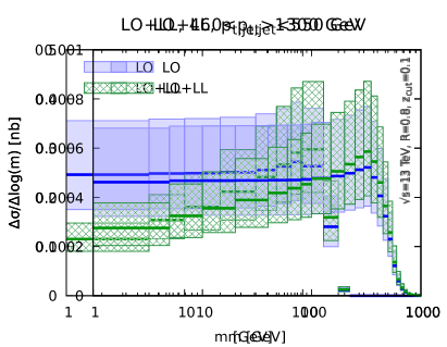
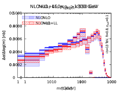
Figure 1: In this figure we show the resummed and matched jet mass distribution in the $460<p_{t,\text{jet}}<550$ GeV transverse momentum bin (on the left), and in the $p_{t,\text{jet}}>1300$ GeV bin (on the right). The top panels show LO+LL, while the bottom panels show NLO+LL.

We now present our results for the resummed and matched jet mass distribution. We pick two representative bins in transverse momentum, namely $460<p_{t,\text{jet}}<550$ GeV and $p_{t,\text{jet}}>1300$ GeV. In Fig. 1 we show the mass distribution in logarithmic bins of the mass:

$$\frac{\Delta\sigma}{\Delta\log m}\equiv\frac{m_{i+1}-m_{i}}{\log\left(m_{i+1}/m_{i}\right)}\frac{\Delta\sigma}{\Delta m},$$ (21)

where $m_{i+1}$ and $m_{i}$ are, respectively, the upper and lower edge of each mass bin. Blue lines with a solid band represent distributions obtained with fixed-order calculations and their uncertainty, while green or red curves with a hatched band are for resummed and matched results obtained using Eq. (18). We estimate the theoretical uncertainty on the matched result by taking the envelope of all the curves obtained by varying the arbitrary scales ($\mu_{\text{R}},\mu_{\text{F}},\mu_{\text{Q}}$) which enter the fixed-order and resummed calculations, as previously detailed. At the top we compare leading order distributions to LO+LL results, while at the bottom we show the NLO curve compared to NLO+LL. The plots on the left are for the lower-$p_{t,\text{jet}}$ bin, while the ones on the right are for the boosted bin. We can see that the normalisation uncertainty is rather large especially when we consider LO distributions. Therefore, it is also interesting to look at normalised distributions, with the normalisation taken to be the jet cross-section in the relevant transverse momentum bin calculated at LO and NLO, respectively for the LO(+LL) and NLO(+LL) results. We show our results for the normalised distributions in Fig. 2.

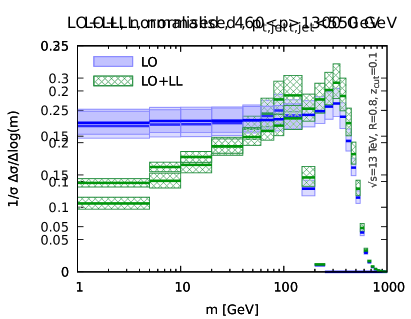
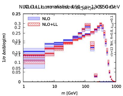
Figure 2: Same as in Fig. 1 but for the normalised distribution.

Since the state-of-the-art NLL studies Frye:2016okc ; Frye:2016aiz neglect the finite $z_{\mathrm{cut}}$ corrections, it is interesting to check their importance. In Fig. 3 we compare the resummed and matched NLO+LL normalised distribution, in red, to an approximation in which the resummation is performed in the $z_{\mathrm{cut}}\to 0$ limit, in grey, for two different transverse momentum bins. From the top plots we can already see that, for $z_{\mathrm{cut}}=0.1$, these effects are small and the two curves fall well within each other’s uncertainty bands. Looking at the bottom plots we can see that these effects are at most a couple of percent at NLO+LL (red curves). For comparison, we also show, in green, the same ratio in the case of the LO+LL result. Note that the bands in the ratio plots represent the uncertainty on the effect, not the overall uncertainty which is of the order of 10%, as can be seen from the top plots. We also note that for a pure LL calculation, finite $z_{\text{cut}}$ effects are found to be of the order of $2\%$, rising to about $5\%$ for $z_{\text{cut}}=0.2$. These findings justify the approximation of Refs. Frye:2016okc ; Frye:2016aiz , which achieved higher-logarithmic accuracy but in the small-$z_{\mathrm{cut}}$ limit. We will see in the next section that the situation radically changes when consider bins in $p_{t,\text{\text{mMDT}}}$.

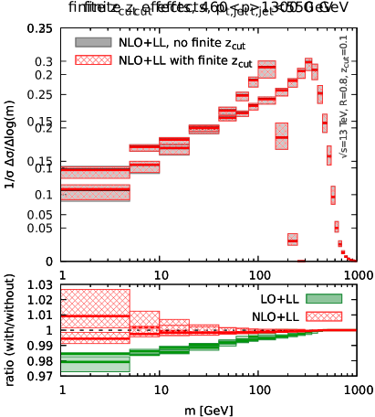
Figure 3: Comparison between the resummed and matched calculation with finite $z_{\mathrm{cut}}$ (red) and the result with the resummation computed in the $z_{\mathrm{cut}}\to 0$ limit. The ratio plots at the bottom show that for $z_{\mathrm{cut}}=0.1$ this type of correction is very small.

Finally, in Fig. 4 we compare two different matching schemes. In particular, we plot the ratio between the NLO+LL distribution obtained with log-$R$ matching Eq. (20) to the one obtained with multiplicative matching Eq. (18), with their respective perturbative uncertainties. We see that the two results are in good agreement and they fall within each other’s scale variation bands.

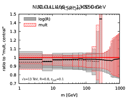
Figure 4: Comparison of the jet mass distribution in two different matching schemes, the multiplicative one Eq. (18) and the log-$R$ one Eq. (20).

4 Jet mass distributions with mMDT using $p_{t,\text{\text{mMDT}}}$

We now consider the alternative option where the mMDT jet mass is measured in bins of $p_{t,\text{\text{mMDT}}}$ rather than $p_{t,\text{jet}}$. We begin our discussion pointing out a known but perhaps under-appreciated fact: the transverse momentum distribution $\frac{d\sigma}{dp_{t,\text{\text{mMDT}}}}$ is not IRC safe, see e.g. Larkoski:2014wba . We then proceed, as before, by discussing our calculation for the jet mass distribution in bins of $p_{t,\text{\text{mMDT}}}$.

4.1 Collinear unsafety (but Sudakov safety) of $p_{t,\text{\text{mMDT}}}$

The mMDT groomer only imposes a cut on the transverse momentum fraction $z$. Therefore, real emissions below $z_{\mathrm{cut}}$ are groomed away without any constraint on the emission angle, resulting in collinear singularities that do not cancel against the corresponding virtual corrections. Thus, the $p_{t,\text{\text{mMDT}}}$ distribution is IRC unsafe and it cannot be computed order-by-order in the strong coupling $\alpha_{s}$, producing a divergence even at the level of the first emission. However, this observable still enjoys the property of Sudakov safety Larkoski:2013paa ; Larkoski:2014wba ; Larkoski:2015lea and it is therefore calculable provided we perform an all-order computation. We note that the situation is instead different if one considers Soft Drop with $\beta>0$, which does regulate the collinear region.

One way to explicitly show the IRC unsafety of the $p_{t,\text{\text{mMDT}}}$ distribution is to study fixed-order distributions in $e^{+}e^{-}$ collisions using the program EVENT2  Catani:1996jh ; Catani:1996vz , for which we can easily control the infrared cut-off scale. In practice, we simulate events at Born level and at ${\cal O}(\alpha_{s})$, including both real emissions and virtual corrections. We cluster the full event with the $e^{+}e^{-}$ version of the anti-$k_{t}$ algorithm with radius $R=0.4$ and select jets with an energy larger than $0.95\sqrt{s}$/2, with $\sqrt{s}=1$ TeV. We note that, at this order in perturbation theory, jets have either one or two constituents. We then run the following $e^{+}e^{-}$ version of mMDT: jets with one constituent are kept untouched, and for jets with two constituents we either keep them intact if $\text{min}(E_{1},E_{2})>z_{\mathrm{cut}}E_{\text{jet}}$, or only keep the most energetic particle otherwise. We use $z_{\mathrm{cut}}=0.1$. We consider the jet cross section for $E>0.95\sqrt{s}/2$ before and after applying mMDT. At Born level, jets after the mMDT procedure are identical to the ungroomed jets. At ${\cal O}(\alpha_{s})$, for an initial jet with an energy above the cut-off, the mMDT jet energy can drop below the cut-off because of a collinear real emission inside the jet that does not pass the mMDT condition. This cannot happen for virtual corrections and so we do expect a leftover singularity.

In numerical codes, both the real and the virtual terms are simulated down to an infrared cut-off so that the numerical result is always finite. When lowering the infrared cut-off parameter the cross section for the ungroomed case is expected to remain constant (modulo small power corrections), while the cross section for mMDT jets is expected to have a residual logarithmic dependence on the cut-off as a consequence of the IRC unsafety. Fig. 5 shows the results of our simulations when varying the infra-red cut-off used in EVENT2 . We indeed clearly see a constant behaviour for the (IRC safe) inclusive cross-section and a logarithmically diverging behaviour for the (IRC unsafe) cross-section after the mMDT procedure.

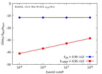
Figure 5: Dependence of the jet cross-section before and after applying mMDT, as a function of the infrared cut-off used in EVENT2 . The cross-section before grooming is stable but the one after grooming diverges logarithmically, thus making IRC unsafety apparent.

Moving back to $pp$ collisions, we study how the nature of the observable, IRC safety for $p_{t,\text{jet}}$ and Sudakov safety for $p_{t,\text{\text{mMDT}}}$, correlates with the size of non-perturbative corrections due to the hadronisation process and to multiple parton interactions, i.e. the underlying event (UE). Although the question of a field-theoretical understanding of non-perturbative corrections and their interplay with substructure algorithms is of great interest, in this study we limit ourselves to a phenomenological approach based on Monte Carlo parton-showers simulations. In order to minimise potential bias due to a particular non-perturbative model, we use a variety of parton showers with different tunes, namely the AUET2 ATLAS:2011gmi tune of Herwig 6.521 Corcella:2000bw ; Corcella:2002jc , the Z2 Field:2010bc and Perugia 2011 Skands:2010ak ; Cooper:2011gk tunes of Pythia 6.428 Sjostrand:2006za , the 4C Corke:2010yf and the Monash 13 tune Skands:2014pea of Pythia 8.223 Sjostrand:2007gs . The results of this study are presented in Fig. 6, where the plot on the left shows the ungroomed $p_{t,\text{jet}}$ spectrum, while the one on the right the $p_{t,\text{\text{mMDT}}}$ distribution. In each plot, we show two sets of curves. The first set (labelled “hadronisation” on the plots) represents, for each Monte Carlo, the ratio between hadron-level and parton-level results, without UE. The second set (labelled “UE”) instead shows the ratio of hadron-level results with and without the UE contribution. The $p_{t,\text{jet}}$ plot shows all the features we would expect from an IRC safe observable. Non-perturbative corrections are suppressed by negative powers of the jet transverse momentum. Moreover, since we are dealing with high-$p_{t}$ jet with a fairly large radius ($R=0.8$) hadronisation corrections are rather small Dasgupta:2007wa . The Sudakov-safe $p_{t,\text{\text{mMDT}}}$ distribution instead exhibits larger hadronisation corrections, which do not appear to be power suppressed Larkoski:2015lea . On the other hand, as perhaps expected in the presence of a groomer, we note that $p_{t,\text{\text{mMDT}}}$ is less sensitive to the UE contribution than $p_{t,\text{jet}}$, especially at moderate transverse momentum. We can therefore expect that $p_{t,\text{\text{mMDT}}}$ will be more resilient against pile-up (not considered here), which has a structure similar to the UE. To cast more light on Sudakov-safe observables, it would be interesting to investigate analytically the structure of hadronisation corrections to the $p_{t,\text{\text{mMDT}}}$ cross-section, using e.g. techniques from Ref. Dasgupta:2007wa .

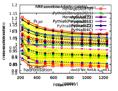
Figure 6: Monte Carlo study of the impact of hadronisation and underlying event (UE) on the ungroomed $p_{t,\text{jet}}$ distribution (on the left) and on the $p_{t,\text{\text{mMDT}}}$ distribution.

In this study we are primarily interested in jet mass distributions, while we only use the jet cross section for normalisation purposes. Measuring a non-vanishing mMDT mass resolves a two-prong structure within the jet, thus acting as an angular cut-off and regulating the collinear divergence. This means that the unnormalised distribution

$$\frac{d\sigma}{d\rho}(\rho;z_{\mathrm{cut}},p_{t1},p_{t2}) =\int_{p_{t1}}^{p_{t2}}dp_{t,\text{\text{mMDT}}}\frac{d^{2}\sigma}{dp_{t,\text{\text{mMDT}}}d\rho},\quad\text{with}\quad\rho=\left(\frac{m}{p_{t,\text{\text{mMDT}}}R}\right)^{2},$$ (22)

is IRC safe. However, as we shall see in the following section, the resulting all-order structure is different compared to the one previously described and rather cumbersome. We also note that, because the difference between $p_{t,\text{jet}}$ and $p_{t,\text{\text{mMDT}}}$ is $\mathcal{O}(z_{\mathrm{cut}})$, if we choose to use $p_{t,\text{\text{mMDT}}}$ we are forced to work at finite $z_{\mathrm{cut}}$.

As a final note, we point out that despite its issues related to IRC safety, $p_{t,\text{\text{mMDT}}}$ shows some interesting properties in perturbative QCD. For example, it is directly related to the “energy loss” distribution computed in Ref. Larkoski:2014wba in the small $z_{\mathrm{cut}}$ limit. Modulo small corrections induced by the running of the coupling, the energy loss distribution — i.e. the $p_{t,\text{\text{mMDT}}}$ distribution at fixed $p_{t,\text{jet}}$ — is independent of $\alpha_{s}$ and of the colour factor of the parton initiating the jet. We discuss this briefly in the context of the $p_{t,\text{jet}}$ jet cross-section in Appendix C.

4.2 Fixed-order structure of the mass distribution

In order to better understand the structure of the mass distribution with $p_{t,\text{\text{mMDT}}}$ we analytically calculate Eq. (22) to LO and NLO, in the collinear limit. We start with a jet of momentum $p_{t,\text{jet}}$. At $\mathcal{O}(\alpha_{s})$ the jet is made of at most two partons. If one of them is groomed away by mMDT, then the resulting groomed jet is massless. Thus, in order to have a non-vanishing mass, the emission must pass the $z_{\mathrm{cut}}$ condition, leading to $p_{t,\text{\text{mMDT}}}=p_{t,\text{jet}}$. Therefore, the LL distribution at LO is the same for the two transverse momentum choices and it reads (see also Ref. Dasgupta:2013via )

$$\rho\frac{d\sigma^{\text{LL,LO}}}{d\rho}(\rho;z_{\mathrm{cut}},p_{t1},p_{t2}) =\int_{p_{t1}}^{p_{t2}}dp_{t,\text{jet}}\left[\sigma_{q}(p_{t,\text{jet}})R^{\prime}_{q}+\sigma_{g}(p_{t,\text{jet}})R^{\prime}_{g}\right],$$ (23)

where $R^{\prime}_{q(g)}$ have been defined in Section 3.1.

The situation changes when we move to NLO. We consider the sum of the double real emission diagrams and the real-virtual contributions, while the double virtual one only gives vanishing masses. At NLO we have different colour structures. For convenience, we explicitly consider the $C_{F}^{2}$ contribution, which originates from the independent emission of two collinear gluons $1$ and $2$ off a quark leg. Analogous results can be obtained for the other colour structures. Because we are interested in the LL contribution, we can order the two emissions in angle, i.e. $\theta_{1}\gg\theta_{2},\theta_{12}$. The relevant contributions correspond to the situation where gluon 2 is real (and dominates the mMDT jet mass) and the large-angle gluon 1 is either real and groomed away, or virtual. The only difference with respect to our calculation in the $p_{t,\text{jet}}$ case (and of Ref. Dasgupta:2013via ) is that here we further have to make sure that the measured $p_{t,\text{\text{mMDT}}}$ falls in the transverse momentum bin under consideration, say ${p_{t1}}<p_{t,\text{\text{mMDT}}}<{p_{t2}}$. Assuming for the moment that ${p_{t1}}<p_{t,\text{jet}}<{p_{t2}}$, we therefore have the additional constraint on the double-real emission contribution that $p_{t,\text{\text{mMDT}}}=(1-z_{1})p_{t,\text{jet}}$ still falls in the same transverse momentum bin. We thus have

$$\rho\frac{d\sigma^{\text{LL,NLO},C_{F}^{2}a}}{d\rho} =\left(\frac{\alpha_{s}C_{F}}{\pi}\right)^{2}\rho\int_{p_{t1}}^{p_{t2}}dp_{t,\text{jet}}\,\sigma_{q}(p_{t,\text{jet}})$$ (24)

$$\cdot\int_{0}^{1}\frac{d\theta_{1}^{2}}{\theta_{1}^{2}}\int_{0}^{1}dz_{1}\,p_{gq}(z_{1})\Big{[}\Theta\left(z_{\mathrm{cut}}>z_{1}\right)\Theta\left((1-z_{1})p_{t,\text{jet}}>p_{t1}\right)-1\Big{]}$$

$$\cdot\int_{0}^{1}\frac{d\theta_{2}^{2}}{\theta_{2}^{2}}\int_{0}^{1}dz_{2}\,p_{gq}(z_{2})\Theta\left(z_{2}>z_{\mathrm{cut}}\right)\Theta\left(1-z_{2}>z_{\mathrm{cut}}\right)\Theta\left(\theta_{1}^{2}>\theta_{2}^{2}\right)\delta\left(\rho-z_{2}\theta_{2}^{2}\right).$$

After some algebra, the distribution in the $\rho<z_{\mathrm{cut}}$ region can be written in terms of the $R_{i}$ functions previously defined

$$\rho\frac{d\sigma^{\text{LL,NLO},C_{F}^{2}a}}{d\rho} =\int_{p_{t1}}^{p_{t2}}dp_{t,\text{jet}}\,\sigma_{q}(p_{t,\text{jet}})R^{\prime}_{q}\Big{[}-R_{q}-R_{q\to g}\Big{]}$$ (25)

$$-\int_{p_{t1}}^{\min\left[p_{t2},\frac{p_{t1}}{1-z_{\mathrm{cut}}}\right]}dp_{t,\text{jet}}\,\sigma_{q}(p_{t,\text{jet}})\;R^{\prime}_{q}\;\frac{\alpha_{s}C_{F}}{\pi}\log\frac{1}{\rho}\int_{1-\frac{p_{t1}}{p_{t,\text{jet}}}}^{z_{\mathrm{cut}}}dz_{1}\,p_{gq}(z_{1}).$$

We note that the first contribution coincides with the expansion of the resummation formula Eq. (8) to second order. However, the second term, proportional to $\alpha_{s}^{2}\log(1/\rho)$, is a new LL contribution that signals the different all-order structure of the mass distribution with $p_{t,\text{\text{mMDT}}}$. Note that we have put a label $a$ in Eqs. (24) and (25) because there is actually a second configuration that contributes, namely when the ungroomed jet has $p_{t,\text{jet}}>p_{t2}$. If the first emission is groomed away, we may end up with $p_{t,\text{\text{mMDT}}}<p_{t2}$, so that this contribution has now leaked into the lower bin. For a quark-initiated jet with two gluon emissions, this results into an additional LL piece:

$$\rho\frac{d\sigma^{\text{LL,NLO},C_{F}^{2}b}}{d\rho} =\int_{p_{t2}}^{\frac{p_{t2}}{1-z_{\mathrm{cut}}}}dp_{t,\text{jet}}\,\sigma_{q}(p_{t,\text{jet}})\;R^{\prime}_{q}\;\frac{\alpha_{s}C_{F}}{\pi}\log\frac{1}{\rho}\int_{1-\frac{p_{t2}}{p_{t,\text{jet}}}}^{z_{\mathrm{cut}}}dz_{1}\,p_{gq}(z_{1}).$$ (26)

4.3 Resummation

In order to resum the groomed jet mass spectrum in the case of the $p_{t,\text{\text{mMDT}}}$ selection we have to generalise the calculation described in the previous section to all orders. Clearly, the situation is much more complicated than the $p_{t,\text{jet}}$ case chiefly because the value of $p_{t,\text{\text{mMDT}}}$ is determined by all the emissions that fail the mMDT condition and therefore our calculation must keep track of them. Because of this complication we are not able to find simple analytic expressions that capture the all-order behaviour, nevertheless we can achieve LL accuracy in the groomed mass distribution using an approach based on generating functionals Ellis:1991qj ; Dokshitzer:1991wu and, in particular, the application of this formalism to the description of the angular evolution of jets with small radius Dasgupta:2014yra ; Dasgupta:2016bnd .

We start by defining an evolution variable which is closely related to the angular scale $\theta$ at which we resolve a jet

$$t=\int_{\theta^{2}}^{1}\frac{d{\theta^{\prime}}^{2}}{{\theta^{\prime}}^{2}}\frac{\alpha_{s}({\theta^{\prime}}p_{t,\text{jet}}R)}{2\pi}=\frac{1}{2\pi\beta_{0}}\,\log\bigg{(}\frac{1}{1+2\alpha_{s}\beta_{0}\log(\theta)}\bigg{)}=\frac{\alpha_{s}}{2\pi}\,\log\bigg{(}\frac{1}{\theta^{2}}\bigg{)}+{\cal{O}}(\alpha_{s}^{2}),$$ (27)

with, as before, $\alpha_{s}=\alpha_{s}(p_{t}R)$. This definition of $t$ includes leading collinear logarithms induced by the running of the QCD coupling when going to small angles. When mMDT (and more generically Soft Drop) recurses to smaller and smaller angular scales, the corresponding value of evolution variable $t$ increases until it reaches a non-perturbative value $t_{\text{max}}$. Thus, by considering successive $1\to 2$ angular-ordered splittings, we can write down LL evolution equations for a generating functional associated to a quark, $Q(x,t)$, or to a gluon $G(x,t)$, where $x$ is the momentum fraction. The relevant evolution equations were derived in Ref. Dasgupta:2014yra . The only difference here is that after each splitting we follow the branch with the highest transverse momentum, as it is appropriate for the mMDT algorithm. We obtain

$$\frac{d}{dt}Q(x,t) =2C_{F}\int_{0}^{1}dz\,p_{gq}(z)\left[Q\left((1-z)x\right)\Theta\left(z<\frac{1}{2}\right)+G\left(zx\right)\Theta\left(z>\frac{1}{2}\right)-Q(x,t)\right],$$ (28a)

$$\frac{d}{dt}G(x,t) =2C_{A}\int_{0}^{1}dz\,\bigg{[}\frac{1}{2}p_{gg}(z)G\big{(}\text{max}(z,1-z)x,t\big{)}+\frac{T_{R}n_{f}}{C_{A}}p_{qg}(z)Q\big{(}\text{max}(z,1-z)x,t\big{)}$$

$$\phantom{=2C_{A}\int_{0}^{1}dz\,[}-p_{xg}(z)G(x,t)\bigg{]}.$$ (28b)

These equations can be implemented numerically under the form of a Monte Carlo generator producing angular-ordered (from large angles to small ones) parton branchings. Compared to the implementation used in Dasgupta:2014yra , the only difference is that the successive branchings follow the hardest of the two partons obtained at the previous step of the showering. We record the angle $\theta$ and momentum fraction $z$ of all the emissions.

In order to obtain the mMDT mass spectrum, two extra ingredients are needed: firstly, we need to impose the mMDT condition and, secondly, we should impose an ordering in invariant mass rather than an ordering in angle. Since mMDT proceeds by declustering a C/A tree, imposing the mMDT condition on our angular-ordered events is trivial: we simply search for the first emission that satisfies $z_{\mathrm{cut}}<z<1-z_{\mathrm{cut}}$. From the momentum fractions of all the previous emissions, i.e. those at larger angles, we can then reconstruct the momentum fraction groomed away by the mMDT procedure and thus $p_{t,\text{\text{mMDT}}}$. Then, once we have reached an emission that passes the mMDT condition, we investigate all the emissions to find the one that dominates the mass. If these emissions have angles $\theta_{i}$, obtained by inverting Eq. (27), and momentum fractions $z_{i}$, we take, to LL accuracy, $\rho=\text{max}_{i}[\text{min}(z_{i},1-z_{i})\theta_{i}^{2}]$. In particular, it is worth pointing out that we can use the momentum fraction $z_{i}$, relative to each branching, instead of the actual momentum of each parton with respect to the initial jet. This is simply because the difference between the two does not generate any logarithmic enhancement. Finally, since the resummation is obtained from a Mote Carlo event generator, it can directly be interfaced with NLOJet++ at Born-level to obtain predictions for the jet mass cross-section.

Before we present matched results, we note that, compared to the resummation done in the previous section for the $p_{t,\text{jet}}$ case, the use of Eq. (27) implies that we are neglecting a factor $z$ in our choice of the scale of the running coupling. This means that we are not including running-coupling effects in the double-logarithmic small-$z_{\mathrm{cut}}$ contributions. This approximation can be explicitly studied in the context of a selection on $p_{t,\text{\text{mMDT}}}$ and we show in Appendix A.2 that this only have a modest impact on the final results.

4.4 Matching and perturbative results

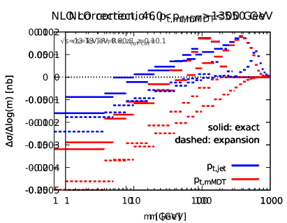
Figure 7: Comparison between the full NLO correction (solid) to the jet mass distribution and the ${\cal O}(\alpha_{s}^{2})$ expansion of the LL resummation (dashed) for both $p_{t,\text{jet}}$ (blue) and $p_{t,\text{\text{mMDT}}}$ (red) in two different transverse momentum bins.

As for the case of the ungroomed $p_{t,\text{jet}}$, an accurate description valid both in the $\rho\ll 1$ region and in the $\rho\sim 1$ region requires the matching of our LL resummation to a fixed-order calculation. As before, the latter is obtained using NLOJet++. We note that at LO, the results are identical to the ones obtained in the $p_{t,\text{jet}}$ case, Section 3.3.

In order to match fixed-order and resummed calculations we have to work out the expansion of the resummed cross-sections to LO and NLO. This can be obtained by expanding Eq. (28) to first and second order in $\alpha_{s}$. In practice, we have found more convenient to reuse here the same code as in Ref. Dasgupta:2014yra , with minor modifications to include additional information about the successive branching angles and momentum fractions as well as simplifications related to the fact that we do not have to include splittings in the soft branch. For fixed $p_{t}$, we have checked our numerical results against an explicit analytic calculation. Note that at NLO, i.e. at ${\cal O}(\alpha_{s}^{2})$, we should include both a contribution coming from two emissions (see also the earlier discussion in Section 4.2) as well as a running-coupling correction coming from the expansion of Eq. (27) to ${\cal O}(\alpha_{s}^{2})$.

We compare the expansion of the LL resummation to ${\cal O}(\alpha_{s}^{2})$ against the exact NLOJet++ NLO correction in Fig. 7, for both $p_{t,\text{jet}}$ (blue) and $p_{t,\text{\text{mMDT}}}$ (red) and for two different transverse momentum bins. We first note that at small mass the expansion of the resummed distribution has the same slope of the corresponding fixed-order, meaning that we do indeed control the ${\cal O}(\alpha_{s}^{2}\log(1/\rho))$ contribution, as expected from our LL calculation. More interestingly, Fig. 7 shows explicitly that the mass distributions obtained in the $p_{t,\text{\text{mMDT}}}$ and $p_{t,\text{jet}}$ cases have different slopes at small mass, i.e. different ${\cal O}(\alpha_{s}^{2}\log(1/\rho))$ contributions. This means that the two distributions already differ at the LL level. The difference in slope is captured by our analytic calculation and is due to the effects already discussed in Section 4.2.

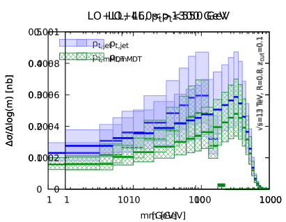
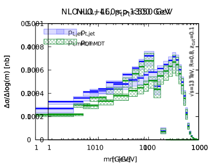
Figure 8: In this figure we compare resummed and matched jet mass distributions in the case of ungroomed $p_{t,\text{jet}}$ selection (blue) or groomed $p_{t,\text{\text{mMDT}}}$ selection (green).

We are now ready to discuss the matching itself. We adopt the multiplicative matching scheme introduced in Eq. (18). Our results are shown in Fig. 8 for the (unnormalised) jet-mass cross-section. The hatched (green) curves are the results obtained for the $p_{t,\text{\text{mMDT}}}$ case and they are compared to the results already obtained in Section 3.3 shown in shaded blue. The plots on the top are for LO+LL, while the ones at the bottom for NLO+LL. We pick the same representative bins in transverse momentum as before, namely $460<p_{t}<550$ GeV and $p_{t}>1300$ GeV, with $p_{t}$ being either $p_{t,\text{\text{mMDT}}}$ or $p_{t,\text{jet}}$. Fig. 7. The cross-sections are smaller for the $p_{t,\text{\text{mMDT}}}$ case than for the $p_{t,\text{jet}}$ case, mostly because the overall inclusive jet cross-section is smaller. This is related to the loss of transverse momentum when applying the mMDT procedure, which is also discussed in Appendix C. We also see, in particular in the NLO+LL results for the high-$p_{t}$ bin, that $p_{t,\text{\text{mMDT}}}$ distributions decrease slightly faster than the $p_{t,\text{jet}}$ ones, at small mass. This feature was already observed in Fig. 7 and it can be attributed to the presence of extra logarithmic contributions, which further suppress the distribution at small values of the mass.

We note that due to the IRC unsafety of the $p_{t,\text{\text{mMDT}}}$ jet cross-section, the normalisation of the fixed-order jet mass distribution is ill-defined. The resummed and matched cross-sections could simply be normalised to unity but we found that this procedure tends to clearly underestimate the size of the perturbative uncertainty and is potentially dangerous as it relies on the computation of the resummed cross-section down to very small masses where non-perturbative effects are dominant. We have therefore decided to present only predictions for the unnormalised distributions.

5 Non-perturbative corrections

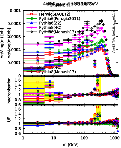
Figure 9: The top plots show the groomed jet mass distribution for $460<p_{t}<550$ GeV, with hadronisation and the underlying event, for different Monte Carlo parton showers. The plot on the left is for the ungroomed $p_{t,\text{jet}}$, while the one of the right for $p_{t,\text{\text{mMDT}}}$. The bottom plots show the ratios hadron-to-parton level and with-to-without the underlying event.

Figure 10: Same as Fig. 9 but for the bin $p_{t}>1300$ GeV.

In this section we perform a Monte Carlo study of non-perturbative contributions considering effects coming from the hadronisation process as well as from the underlying event. In order to study non-perturbative corrections to the jet mass distribution we consider the same set of Monte Carlo tunes used for studying the $p_{t}$ spectra in Section 4. As usual, we consider two representative transverse momentum bins. In Fig. 9 we consider $460<p_{t}<550$ GeV, while in Fig. 10 we consider $p_{t}>1300$ GeV. In both cases, the plots on the left refer to the ungroomed $p_{t,\text{jet}}$ selection, while the ones on the right refer to the $p_{t,\text{\text{mMDT}}}$ case.

In the top plots we show the (unnormalised) jet mass distributions as obtained from each Monte Carlo program. The striking feature is the huge discrepancy between these results, even at large masses. In particular, the predictions obtained with the most recent Pythia 8 tunes appear to be a factor of 2 larger than the other tunes in the region of interest for this study. This performance of standard parton shower tools, worrisome at first glance, should be put in parallel with our LO+LL results (see e.g. Fig. 8) which exhibit a similar uncertainty band. This indicates the need to match the parton shower with NLO fixed-order matrix elements.

In the bottom plots of Figs. 9 and 10 we instead show, for each Monte Carlo, the ratio of hadron-to-parton level results (labelled “hadronisation”) and the ratio with-to-without the underlying event contribution (labelled “UE”). We first note that in both the $p_{t,\text{jet}}$ and $p_{t,\text{\text{mMDT}}}$ selection cases, the groomed mass distribution has very small sensitivity to the underlying event, as we expect from mMDT being an (aggressive) groomer. This contribution becomes more sizeable at large masses essentially because the effective jet radius becomes larger. Moreover, this effect is more visible in the moderate $p_{t}$ bin since the power-suppression in the hard scale of the process becomes weaker. Hadronisation corrections have instead a different shape for the $p_{t,\text{jet}}$ and $p_{t,\text{\text{mMDT}}}$ selections, most likely stemming from the different properties of the underlying transverse momentum distribution. For the $p_{t,\text{jet}}$ case, hadronisation corrections are sizeable in the low mass bins, with a peculiar peak in the 5-10 GeV bin, and at very large masses, close to the end-point region. For both small and large masses, this also comes with a larger spread of the hadronisation corrections across the generators and tunes. However, there exists a rather large region in mass, increasing in size as $p_{t,\text{jet}}$ grows, where these contributions are genuinely small. Hadronisation corrections have a similar size in the $p_{t,\text{\text{mMDT}}}$ selection case. This is not unexpected because the mass distribution is itself IRC safe. However, they do exhibit a rather different shape. They come with opposite sign at small masses and appear to be non-negligible in a wider region of the mass distribution, similarly to what was already noticed in Section 4.1 for the jet cross-section.

Given the large kinematic range over which the non-perturbative corrections appear to be small, upcoming LHC data could bring valuable constraints on the perturbative aspects of parton showers. Additionally, the behaviour at low mass, with very little sensitivity to the underlying event, could help constraining hadronisation models. For example, measurements on both quark and gluon-enriched jet samples would be complementary to the quark-dominated LEP data currently used to tune hadronisation models Badger:2016bpw ; QuarkGluon .

In practice, for this study, we use the above Monte Carlo results to estimate the size and the uncertainty of non-perturbative corrections on the groomed mass distribution. For each Monte Carlo generator and tune we construct the ratio particle-level, i.e. hadronisation with UE, to parton-level, in each mass and transverse momentum bin. We take the average value of this ratio as a correction factor to apply to the perturbative NLO+LL results obtained in the previous sections. We take the envelope of the corrections across different generators and tunes as an estimate of the non-perturbative uncertainty, which we add in quadrature to the perturbative uncertainty. We consider this solution an acceptable and rather conservative estimate of non-perturbative contributions, lacking a detailed, field-theoretical study of these corrections in the presence of grooming algorithms.

6 Final results

We can now present our final results for the groomed jet mass distribution for both the $p_{t,\text{jet}}$ and $p_{t,\text{\text{mMDT}}}$ selection. Our perturbative results, which are accurate to NLO+LL, are multiplied by a bin-by-bin (in both mass and transverse momentum) non-perturbative correction factor obtained from Monte Carlo parton showers. The total uncertainty is taken as the sum in quadrature of the perturbative and non-perturbative uncertainties. The former is obtained by varying renormalisation, factorisation, and resummation scales as described in Section 3 and taking the envelope of the result; the latter by considering the envelope of the five different Monte Carlo generators and tunes.

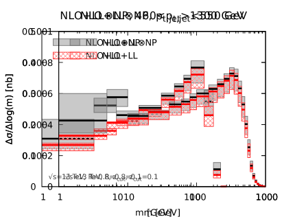
Figure 11: Final results for the jet mass distribution in the case of the ungroomed $p_{t,\text{jet}}$ selection. The perturbative calculation is performed at NLO+LL and non-perturbative corrections are included as a multiplicative factor obtained from Monte Carlo parton showers. Perturbative uncertainties are obtained varying renormalisation, factorisation and resummation scales as detailed in Section 3. Non-perturbative uncertainties are obtained considering the spread of five different Monte Carlo tunes, as detailed in Section 5. Perturbative and non-perturbative uncertainties are added in quadrature.

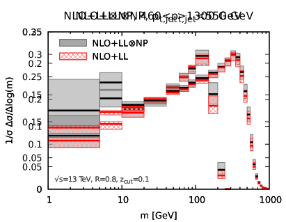
Figure 12: Final results at NLO+LL, with non-perturbative corrections, for the normalised jet mass distribution, in the case of the ungroomed $p_{t,\text{jet}}$ selection.

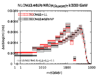
Figure 13: Final results at NLO+LL, with non-perturbative corrections, for the $p_{t,\text{\text{mMDT}}}$ selection.

Fig. 11 and Fig. 12 show the results (in black, with grey uncertainty bands) for the ungroomed $p_{t,\text{jet}}$ selection in the two representative transverse momentum bins: $460<p_{t,\text{jet}}<550$ GeV and $p_{t,\text{jet}}>1300$ GeV. The former is the jet mass distribution, while the latter is normalised to the NLO jet cross-section in the appropriate transverse momentum bin. Similarly, in Fig. 13 we show our final results for the $p_{t,\text{\text{mMDT}}}$ selection. As discussed in the paper, the NLO jet cross section is not well-defined in this case, so we only present unnormalised distributions. For comparison, we also show in red the purely perturbative NLO+LL results with their uncertainties. As previously noted, non-perturbative corrections are sizeable (with large uncertainties) in the first few mass bins ($m\lesssim 10$ GeV) and at very large masses, close to the end-point region. Nevertheless, there exists a region in mass, which increases in size as $p_{t,\text{jet}}$ grows, where non-perturbative effects are genuinely small and a meaningful comparisons between experiments and perturbation theory can be performed. However, we have found that, when we consider normalised distributions in Fig. 12, the uncertainty related to these non-perturbative contributions is, at best, of the same order as the NLO+LL perturbative calculation.

The above results clearly demonstrate the value of jet substructure algorithms to perform phenomenological studies in QCD. In particular, the region in mass where non-perturbative contributions are genuinely small offers an opportunity to test the modeling of perturbative radiation in analytic resummations and parton showers. In that respect, one could even consider the possibility to use experimental data in this mass region for a novel measurement of the strong coupling. On the other hand, the lower mass bins, which are sensitive to hadronisation but have small UE contaminations, can be used to test (and tune) the hadronisation models of Monte Carlo event generators. To this purpose, it will be also interesting to extend this analysis to different jet shapes and angularities, and to different processes, e.g.  Z+jet, which have different sensitivity to QCD radiation, both at the perturbative and non-perturbative level. Furthermore, while the $p_{t,\text{jet}}$ selection is under better theoretical control and should be amenable to a higher logarithmic accuracy, we think that the $p_{t,\text{\text{mMDT}}}$ case also offers many interesting physics opportunities. While the jet mass distribution is IRC safe in both cases, the underlying $p_{t,\text{\text{mMDT}}}$ itself is not. Detailed studies of these types of observables will improve our understanding of Sudakov safety. Furthermore, the two transverse-momentum selections exhibit different sensitivities to non-perturbative effects (especially hadronisation). Such a measurement could therefore shed some light on power corrections for Sudakov-safe observables and be of further help for Monte Carlo tuning.

7 Conclusions

In this paper we have considered the production of hadronic jets in proton-proton collisions and studied the invariant mass distributions of groomed jets, focusing on the mMDT algorithm, sometimes also referred to as Soft Drop with the angular exponent set to zero. Our calculation is double-differential in jet mass and transverse momentum and fully takes into account the kinematic cuts of an upcoming CMS measurement at $\sqrt{s}=13$ TeV. We present our results as jet mass distributions in different transverse-momentum bins.

Jet mass distributions receive logarithmic corrections originating from the emissions of soft and/or collinear partons. However, the presence of a grooming algorithm mitigates the contributions from the soft region of phase-space. The resulting mMDT mass distribution is single-logarithmic with the logarithmic enhancements only stemming from the hard-collinear region. We have resummed this contribution to LL accuracy. In doing so we have lifted the small-$z_{\mathrm{cut}}$ approximation which has been used in other studies aimed at a higher logarithmic accuracy Frye:2016okc ; Frye:2016aiz . In order to also describe the high-mass tail of the distribution we match to fixed-order matrix elements at NLO using the program NLOJet++.

We have considered two different choices for the transverse momentum selection. The first option consists in selecting and binning the jets according to their transverse momentum before grooming, namely $p_{t,\text{jet}}$, while in the second one the transverse momentum after grooming $p_{t,\text{\text{mMDT}}}$ is used. We note that a calculation performed in the small-$z_{\mathrm{cut}}$ limit cannot resolve this difference, as the two are equal at $z_{\text{cut}}=0$.

We have found that the $p_{t,\text{jet}}$ selection is better suited for theoretical calculations and the resulting resummation has a relatively simple form that can be, in principle, extended to higher-logarithmic accuracy. Moreover, for the typical choice $z_{\mathrm{cut}}=0.1$, finite $z_{\mathrm{cut}}$ corrections, although formally entering already at LL accuracy, appear to be very small. This justifies the small-$z_{\mathrm{cut}}$ approximation used in Refs. Frye:2016okc ; Frye:2016aiz to achieve higher logarithmic accuracy. However, the finite $z_{\text{cut}}$ corrections would inevitably increase for larger values of $z_{\text{cut}}$. Also, it would be interesting to achieve a complete picture at NLL accuracy, including the finite $z_{\text{cut}}$ corrections, even though our findings in this paper suggest that the latter would be small. We have also found that logarithms of $z_{\mathrm{cut}}$ give a non-negligible contribution, thus indicating the necessity of their resummation. We have also studied the perturbative uncertainty of our calculation, observing that matching to NLO greatly reduces the theoretical uncertainty especially in the case of unnormalised distributions. Finally, we have studied non-perturbative contributions from hadronisation and the underlying event using different Monte Carlo parton showers. Non-perturbative effects are reduced compared to the ungroomed jet mass and only remain sizeable at low mass, where hadronisation dominates, or at very large masses, close to the end-point of the distribution.

The $p_{t,\text{\text{mMDT}}}$ selection has instead more theoretical issues but it can also present some advantages from a phenomenological viewpoint. The main theoretical complication stems from the fact that the $p_{t,\text{\text{mMDT}}}$ jet spectrum is not IRC safe, but only Sudakov safe. The jet mass distribution is itself safe, with the mass acting as a regulator for collinear emissions, but the inclusive $p_{t,\text{\text{mMDT}}}$ cross-section is only Sudakov safe. Due to the complicated flavour structure of the all-order resummation, we were only able to arrive at a numerical resummation of the LL contributions. A possible extension of our results to a higher logarithmic accuracy is therefore expected to be difficult, even in principle. From a phenomenological viewpoint, it would be interesting to see whether the slightly smaller sensitivity to the underlying event of the $p_{t,\text{\text{mMDT}}}$ choice implies a smaller sensitivity to pileup.

To summarise, in this work we have derived theoretical predictions for the invariant mass distribution of jets groomed with mMDT, including a study of the perturbative and non-perturbative theoretical uncertainties. The situation where distributions are computed in bins of the initial (ungroomed) jet $p_{t}$ exhibit a simpler analytic structure, compared to the case where the binning is done using the groomed jet $p_{t}$. This means that the former is more likely to be amenable to a theoretical calculation with higher logarithmic accuracy. We look forward to comparing our calculations to upcoming LHC measurements and extend our predictions to additional observables.

Appendix A Details of the analytic calculation

In this Appendix we give more detail about the calculations of the resummation functions $R_{i}$ introduced in Section 3.1.

A.1 Resummed exponents

The splitting functions introduced in Eqs. (9) are defined as

$$p_{gq} = \dfrac{1+(1-z)^{2}}{2z},$$ (29)

$$p_{qg} = \dfrac{1}{2}\big{(}z^{2}+(1-z)^{2}\big{)},$$ (30)

$$p_{gg} = \dfrac{2(1-z)}{z}+z(1-z),$$ (31)

and we have also defined the following combination

$$p_{xg}\equiv\dfrac{1}{2}p_{gg}+\dfrac{T_{R}n_{f}}{C_{A}}p_{qg}.$$ (32)

The running coupling used in Eqs. (9) is computed at the one-loop accuracy, namely

$$\alpha_{s}(\kappa)=\frac{\alpha_{s}(Q)}{1+2\alpha_{s}(Q)\beta_{0}\log\frac{\kappa}{Q}}\ .$$ (33)

Our results are expressed in terms of $\alpha_{s}=\alpha_{s}(R\,p_{t,\text{jet}})$, evolved from $\alpha_{s}(m_{Z})=0.118$ with a two-loop approximation ($n_{f}=5$). Note that for the minimal jet mass of 1 GeV that we consider in this paper and the variations of the renormalisation and resummation scales, $\mu_{R}$ and $\mu_{Q}$, our perturbative results always remain above the Landau pole. We could decide to freeze the coupling at a scale $\mu_{\text{NP}}$ that we would vary around 1 GeV, and hence obtain an uncertainty associated to using perturbative QCD in a region sensitive to non-perturbative effects. However this effect should be included already in our estimate of the non-perturbative effects via the Monte-Carlo simulations discussed in Section 5.

To obtain the results presented in the main text, we have written the splitting functions entering the flavour-diagonal contributions as a sum of two different contributions:

$$p_{gq}(z) =\frac{C_{F}}{z}\Theta(z<e^{B_{q}})+p_{gq}^{\text{(finite)}}(z),$$ (34a)

$$p_{xg}(z) =\frac{C_{A}}{z}\Theta(z<e^{B_{g}})+p_{xg}^{\text{(finite)}}(z).$$ (34b)

The cut-off at $z=e^{B_{i}}$ is such that the leftover finite part only generates power corrections in $z_{\mathrm{cut}}$ while the $\log(1/z_{\mathrm{cut}})$ and constant terms are included in the first terms proportional to $1/z$. Note that this will naturally produce distributions with an end-point at $\rho=e^{B_{i}}$. That said, the contribution from the first term can be integrated straightforwardly and gives the ${\mathcal{R}}_{i}$ function given in Eq. (10).

Next, we consider the contributions coming from the second term in Eq. (34), as well as from the flavour-changing contributions, which will be power-suppressed in $z_{\mathrm{cut}}$. For these, we can safely ignore the factor $z$ in both the argument of $\alpha_{s}$ and the constraint $\Theta(z\theta^{2}>\rho)$. The $z$ and $\theta^{2}$ integration then factorise to give

$$\text{finite part: }\int_{\rho}^{z_{\mathrm{cut}}}\frac{d\theta^{2}}{\theta^{2}}\frac{\alpha_{s}(\theta p_{t,\text{jet}}R)}{\pi}\>\int_{z_{\text{min}}}^{z_{\text{max}}}dz\,p^{\text{(finite)}}_{ij}(z),$$ (35)

where the integration boundaries $z_{\text{min}}$ and $z_{\text{max}}$ depend on which matrix element we consider and should match those imposed by the mMDT conditions in Eq. (9). Once again, to our accuracy, there is some freedom in the choice of the upper integration boundary of the $\theta^{2}$ integration. Setting it to $z_{\mathrm{cut}}$ ensures that there are no corrections beyond the transition point $\rho=z_{\mathrm{cut}}$. Note that neglecting the finite $z_{\mathrm{cut}}$ effects is equivalent to keeping only the contribution from $\mathcal{R}_{i}$ while neglecting the contribution from Eq. (35).

A.2 Impact of the $z$ factor in the scale of the running coupling

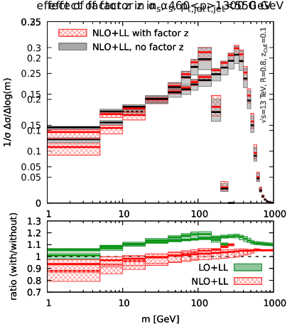
Figure 14: Comparison of the jet mass distribution with and without the resummation of logarithmic corrections in $z_{\mathrm{cut}}$ originating from the running of the strong coupling. We note that these effects are sizeable, although still within the theoretical uncertainty.

If the parameter $z_{\mathrm{cut}}$ is chosen to be rather small, finite-$z_{\mathrm{cut}}$ corrections are negligible but logarithmic corrections can become relevant. The resummation of the leading-logarithmic corrections in $z_{\mathrm{cut}}$ is relatively straightforward and it was discussed in Ref. Dasgupta:2013ihk (see also Refs. Frye:2016okc ; Frye:2016aiz ). Firstly, successive gluon emissions must be ordered in mass rather than in angle. Secondly, the argument of the QCD running coupling should be taken as $k_{t}=z\theta p_{t,\text{jet}}R$ (at least for the calculation of $\mathcal{R}_{i}$). Both effects are included in our calculation. However, to LL accuracy (in $\rho)$ the argument of the running coupling could more simply be chosen as $\theta p_{t,\text{jet}}R$. This choice leads to simpler analytic expressions and is what we naturally obtain when we consider bins of $p_{t,\text{\text{mMDT}}}$, see Eq. (27). It is therefore of some interest to investigate how neglecting the factor $z$ in the argument of the running coupling affects our findings. In this case, the $\mathcal{R}_{i}$ functions in Eq. (11) become

$$\widetilde{\mathcal{R}}_{i}=\frac{1}{\pi\alpha_{s}\beta_{0}^{2}}\Big{[}W\big{(}1+\alpha_{s}\beta_{0}(\log(\rho)-B_{i})\big{)}-W\big{(}1+\alpha_{s}\beta_{0}\log(\rho/z_{m})\big{)}-\alpha_{s}\beta_{0}(\log(z_{m})-B_{i})\Big{]}.$$ (36)

In Fig. 14 we show the impact of these corrections on the normalised matched distributions. Remembering that the uncertainty on the lower panels is the actual uncertainty on the ratio, we see that the effects are genuinely present. However, they remain within our overall theoretical uncertainties shown on the mass distribution (upper plots).

Appendix B End-point of the $\rho$ distribution

As discussed in Section 3.2, we have modified the argument $\log\left(1/\rho\right)$ to take into account end-point effects i.e. the fact that $\rho$ has a maximum value $\rho_{\max}$ for a jet with transverse momentum $p_{t}$ and radius $R$. In this Appendix, we give the details of the computation of $\rho_{\max}$ at LO and NLO.

Figure 15: Configurations with maximal mass for LO (left) and NLO (right).

At LO, where we have two partons $p_{1}$ and $p_{2}$ in the jet, the calculation is straightforward. The mass of the jet, and therefore $\rho$, will be maximal when the final partons are as distant as possible, but are still clustered into a single jet. Let us first work in the small-angle limit. Then, the angular distance between the two partons is $\theta_{12}=R$, as shown in the left plot of Fig. 15. If the two partons carry a transverse momentum $p_{t1}=xp_{t}$ and $p_{t2}=(1-x)p_{t}$, respectively, the jet mass is given by

$$m^{2}=p_{t}^{2}R^{2}x(1-x).$$ (37)

This is maximal when the momentum is equally distributed between the two partons, $x=1/2$, for which we have $\rho^{\text{(small-$R$)}}_{\max,\text{LO}}=1/4$. If we relax our small-angle approximation, we should take into account that the mass of the system of two partons separated by a distance $R$ will depend on their orientation in the rapidity-azimuthal angle plane. It is straightforward to include this in the above analytic calculation and we find that $\rho$ is maximal when the two partons have the same rapidity, leading to $\rho_{\max,\text{LO}}=R^{-2}\tan^{2}\frac{R}{2}$ Dasgupta:2012hg . For our choice of $R=0.8$, this gives $\rho_{\max,\text{LO}}=0.279303$.

At NLO, the same reasoning applies but is complicated by the presence of one more parton in the jet. We start again by considering the small-$R$ limit. Remembering that the three partons must be clustered into a single anti-$k_{t}$ jet of radius $R$, we can assume, without loss of generality, that $p_{1}$ and $p_{2}$ are the first pair of partons to be clustered into a subjet with momentum $p_{12}$, with $p_{12}$ then clustered with parton $p_{3}$. In order to have all 3 partons clustered into a single jet, we must have $\theta_{12}\leq R$ and $\theta_{(12)3}\leq R$. We define $\varphi$ as being the angle between $\theta_{12}$ and $\theta_{(12)3}$, as shown in the right plot of Fig. 15, and we parametrise the momentum fractions of the partons as

$$z_{1}=xt,\qquad z_{2}=x(1-t),\qquad z_{3}=1-x.$$ (38)

Since $\theta_{(12)1}=(1-t)\theta_{12}$ and $\theta_{(12)2}=t\theta_{12}$, we have

$$\theta_{13}^{2} = (1-t)^{2}\theta_{12}^{2}+\theta_{(12)3}^{2}+2(1-t)\theta_{12}\theta_{(12)3}\cos\varphi,$$ (39)

$$\theta_{23}^{2} = t^{2}\theta_{12}^{2}+\theta_{(12)3}^{2}+2t\theta_{12}\theta_{(12)3}\cos\varphi.$$ (40)

The jet mass is then found to be

$$m^{2}=p_{t}^{2}(z_{1}z_{2}\theta_{12}^{2}+z_{1}z_{3}\theta_{13}^{2}+z_{2}z_{3}\theta_{23}^{2})=p_{t}^{2}xt(1-t)\theta_{12}^{2}+p_{t}^{2}x(1-x)\theta_{(12)3}^{2}.$$ (41)

This is maximal for $\theta_{12}=\theta_{(12)3}=R$ and momentum equally distributed between $p_{1}$ and $p_{2}$, i.e. $t=1/2$, in which case we have

$$m^{2}=p_{t}^{2}R^{2}x\left(\dfrac{5}{4}-x\right).$$ (42)

The maximum jet mass is thus reached for $x=5/8$, which corresponds to $\rho^{\text{(small-$R$)}}_{\max,\text{NLO}}=25/64$. If we lift the small-$R$ approximation, the situation becomes more complex since the mass now depends explicitly on the angle $\varphi$ as well as on an additional overall rotation angle $\psi$ of the 3-parton system. One can write analytic expressions for the jet mass and transverse-momentum conservation and, for given values of $\varphi$ and $\psi$ we can maximise the mass. The maximisation over $\varphi$ and $\psi$ has been done numerically — imposing that $\Delta R_{12}<R$ and $\Delta R_{(12)3}<R$ as required by the clustering — and we find is $\rho_{\max,\text{NLO}}=0.44974$ for $R=0.8$.

Appendix C LL predictions for the $p_{t,\text{\text{mMDT}}}$ jet cross-section

Before investigating in detail the double-differential cross-section $d^{2}\sigma/(dp_{t,\text{\text{mMDT}}}\,dm)$, one might be tempted to study the jet cross-section, $d\sigma/dp_{t,\text{\text{mMDT}}}$. Despite looking simpler, the latter is actually plagued with the issue of IRC unsafety, while for the former, the measured jet mass acts as a regulator of the collinear divergence. In this Appendix, we therefore briefly depart from our study of the double-differential mass distribution to concentrate instead on the Sudakov-safe $d\sigma/dp_{t,\text{\text{mMDT}}}$.

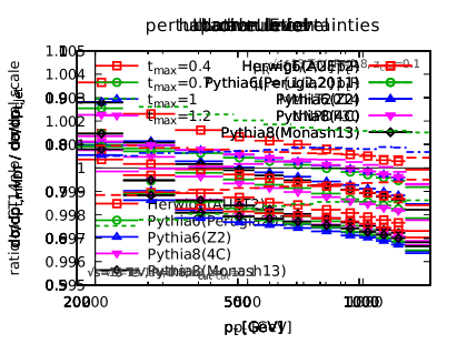
Figure 16: Ratio of the jet cross-section $d\sigma/dp_{t,\text{\text{mMDT}}}$, binned in the groomed jet $p_{t}$, to the standard jet cross-section $d\sigma/dp_{t,\text{jet}}$. The results of Monte-Carlo simulations performed with different generators and tunes are shown in the top-left, bottom-left and bottom-right plots, respectively for simulations at parton-level, hadron-level without UE, and hadron-level including UE. The top-right plot instead shows our LL analytic results.

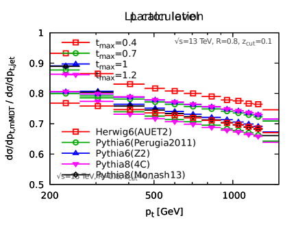
Figure 17: Theoretical uncertainties on the ratio $(d\sigma/dp_{t,\text{\text{mMDT}}})/(d\sigma/dp_{t,\text{jet}})$. Uncertainties associated with the choice of the renormalisation and factorisation scales as well as with the choice of PDF are shown relative to the ratio obtained for the central scale choice and our default CT14nlo PDF set.

The results of both our LL calculation and of Monte Carlo simulations at different levels are presented in Fig. 16, for the ratio $(d\sigma/dp_{t,\text{\text{mMDT}}})/(d\sigma/dp_{t,\text{jet}})$. We can make two main observations: firstly, our LL calculation provides a good description of what is observed at parton level. Secondly, as already noticed in Fig. 6, hadronisation effects are sizeable while UE correction are more modest. Additionally, Fig. 16 shows the dependence of our LL calculation when varying the value $t_{\text{max}}$ of $t$ at which we stop parton branchings. For all the results presented in the main body of the paper, we have adopted $t_{\text{max}}=1.2$ which shows stable results in Fig. 16.

From a theoretical viewpoint, $d\sigma/dp_{t,\text{\text{mMDT}}}$ can be viewed as the convolution of the jet spectrum $d^{2}\sigma/dp_{t,\text{jet}}$ with the “jet energy drop”, $1/\sigma\,d\sigma/d\Delta_{E}$ distribution, computed in the original Soft Drop paper Larkoski:2014wba at LL accuracy in $\Delta_{E}$, neglecting finite $z_{\mathrm{cut}}$ corrections. For the specific case of mMDT, i.e. the limit $\beta\to 0$ of Soft Drop, we found the remarkable property that, modulo running coupling corrections, the energy drop spectrum is independent of $\alpha_{s}$ and of the flavour of the parton initiating the jet. It is therefore interesting to study the theoretical uncertainty of our LL calculation of $d\sigma/dp_{t,\text{\text{mMDT}}}$, as measured from scale variation. This is shown in Fig. 17. The observed theoretical uncertainty is indeed very small, well below 1%. This should be contrasted with the much larger spread of the parton-level results from our Monte Carlo simulations, the top-left panel of Fig. 16. This could be related to subleading effects not captured by scale variation, or to effects of finite shower cut-off, seen also in our LL calculation when varying $t_{\text{max}}$. The question of the power corrections to the $p_{t,\text{\text{mMDT}}}$ cross-section, and to Sudakov-safe observables in general, is therefore interesting both from the point of view of Monte-Carlo simulations and all-order calculations.

References

- (1) M. H. Seymour, Searches for new particles using cone and cluster jet algorithms: A Comparative study, Z. Phys. C62 (1994) 127–138.
- (2) J. M. Butterworth, B. E. Cox, and J. R. Forshaw, scattering at the CERN LHC, Phys. Rev. D65 (2002) 096014, [hep-ph/0201098].
- (3) A. Abdesselam, E. B. Kuutmann, U. Bitenc, G. Brooijmans, J. Butterworth, et al., Boosted objects: A Probe of beyond the Standard Model physics, Eur.Phys.J. C71 (2011) 1661, [arXiv:1012.5412].
- (4) A. Altheimer, S. Arora, L. Asquith, G. Brooijmans, J. Butterworth, et al., Jet Substructure at the Tevatron and LHC: New results, new tools, new benchmarks, J.Phys. G39 (2012) 063001, [arXiv:1201.0008].
- (5) A. Altheimer et al., Boosted objects and jet substructure at the LHC. Report of BOOST2012, held at IFIC Valencia, 23rd-27th of July 2012, Eur. Phys. J. C74 (2014), no. 3 2792, [arXiv:1311.2708].
- (6) D. Adams et al., Towards an Understanding of the Correlations in Jet Substructure, Eur. Phys. J. C75 (2015), no. 9 409, [arXiv:1504.00679].
- (7) ATLAS Collaboration, Search for resonances with boson-tagged jets in 15.5 fb-1 of collisions at TeV collected with the ATLAS detector, Tech. Rep. ATLAS-CONF-2016-055, 2016.
- (8) ATLAS Collaboration, G. Aad et al., Search for high-mass diboson resonances with boson-tagged jets in proton-proton collisions at TeV with the ATLAS detector, JHEP 12 (2015) 055, [arXiv:1506.00962].
- (9) CMS Collaboration, V. Khachatryan et al., Search for massive resonances in dijet systems containing jets tagged as W or Z boson decays in pp collisions at = 8 TeV, JHEP 08 (2014) 173, [arXiv:1405.1994].
- (10) C. F. Berger, T. Kúcs, and G. Sterman, Event shape / energy flow correlations, Phys. Rev. D 68 (2003) 014012, [hep-ph/0303051].
- (11) S. D. Ellis, C. K. Vermilion, J. R. Walsh, A. Hornig, and C. Lee, Jet Shapes and Jet Algorithms in SCET, JHEP 1011 (2010) 101, [arXiv:1001.0014].
- (12) A. J. Larkoski, G. P. Salam, and J. Thaler, Energy Correlation Functions for Jet Substructure, JHEP 1306 (2013) 108, [arXiv:1305.0007].
- (13) I. Moult, L. Necib, and J. Thaler, New Angles on Energy Correlation Functions, JHEP 12 (2016) 153, [arXiv:1609.07483].
- (14) M. Seymour, Jet shapes in hadron collisions: Higher orders, resummation and hadronization, Nucl.Phys. B513 (1998) 269–300, [hep-ph/9707338].
- (15) J. Thaler and K. Van Tilburg, Identifying Boosted Objects with N-subjettiness, JHEP 1103 (2011) 015, [arXiv:1011.2268].
- (16) J. Thaler and K. Van Tilburg, Maximizing Boosted Top Identification by Minimizing N-subjettiness, JHEP 1202 (2012) 093, [arXiv:1108.2701].
- (17) G. P. Salam, L. Schunk, and G. Soyez, Dichroic subjettiness ratios to distinguish colour flows in boosted boson tagging, JHEP 03 (2017) 022, [arXiv:1612.03917].
- (18) M. Dasgupta, A. Powling, L. Schunk, and G. Soyez, Improved jet substructure methods: Y-splitter and variants with grooming, JHEP 12 (2016) 079, [arXiv:1609.07149].
- (19) A. J. Larkoski, I. Moult, and D. Neill, Analytic Boosted Boson Discrimination, JHEP 05 (2016) 117, [arXiv:1507.03018].
- (20) A. J. Larkoski, I. Moult, and D. Neill, Power Counting to Better Jet Observables, JHEP 12 (2014) 009, [arXiv:1409.6298].
- (21) A. J. Larkoski, I. Moult, and D. Neill, Building a Better Boosted Top Tagger, Phys. Rev. D91 (2015), no. 3 034035, [arXiv:1411.0665].
- (22) J. M. Butterworth, A. R. Davison, M. Rubin, and G. P. Salam, Jet substructure as a new Higgs search channel at the LHC, Phys. Rev. Lett. 100 (2008) 242001, [arXiv:0802.2470].
- (23) D. Krohn, J. Thaler, and L.-T. Wang, Jet Trimming, JHEP 1002 (2010) 084, [arXiv:0912.1342].
- (24) S. D. Ellis, C. K. Vermilion, and J. R. Walsh, Techniques for improved heavy particle searches with jet substructure, Phys.Rev. D80 (2009) 051501, [arXiv:0903.5081].
- (25) S. D. Ellis, C. K. Vermilion, and J. R. Walsh, Recombination Algorithms and Jet Substructure: Pruning as a Tool for Heavy Particle Searches, Phys.Rev. D81 (2010) 094023, [arXiv:0912.0033].
- (26) A. J. Larkoski, S. Marzani, G. Soyez, and J. Thaler, Soft Drop, JHEP 1405 (2014) 146, [arXiv:1402.2657].
- (27) M. Dasgupta, A. Fregoso, S. Marzani, and G. P. Salam, Towards an understanding of jet substructure, JHEP 09 (2013) 029, [arXiv:1307.0007].
- (28) M. Dasgupta, A. Fregoso, S. Marzani, and A. Powling, Jet substructure with analytical methods, Eur. Phys. J. C73 (2013), no. 11 2623, [arXiv:1307.0013].
- (29) ATLAS Collaboration, G. Aad et al., Jet mass and substructure of inclusive jets in TeV collisions with the ATLAS experiment, JHEP 1205 (2012) 128, [arXiv:1203.4606].
- (30) CMS Collaboration Collaboration, S. Chatrchyan et al., Studies of jet mass in dijet and W/Z + jet events, JHEP 1305 (2013) 090, [arXiv:1303.4811].
- (31) A. J. Larkoski, S. Marzani, and J. Thaler, Sudakov Safety in Perturbative QCD, Phys. Rev. D91 (2015), no. 11 111501, [arXiv:1502.01719].
- (32) C. Frye, A. J. Larkoski, M. D. Schwartz, and K. Yan, Precision physics with pile-up insensitive observables, arXiv:1603.06375.
- (33) C. Frye, A. J. Larkoski, M. D. Schwartz, and K. Yan, Factorization for groomed jet substructure beyond the next-to-leading logarithm, JHEP 07 (2016) 064, [arXiv:1603.09338].
- (34) S. Rappoccio. private communications, 2017.
- (35) A. J. Larkoski and J. Thaler, Unsafe but Calculable: Ratios of Angularities in Perturbative QCD, JHEP 1309 (2013) 137, [arXiv:1307.1699].
- (36) Y. L. Dokshitzer, G. Leder, S. Moretti, and B. Webber, Better jet clustering algorithms, JHEP 9708 (1997) 001, [hep-ph/9707323].
- (37) M. Wobisch and T. Wengler, Hadronization corrections to jet cross-sections in deep inelastic scattering, hep-ph/9907280.
- (38) M. Dasgupta and G. P. Salam, Resummation of non-global QCD observables, Phys. Lett. B512 (2001) 323–330, [hep-ph/0104277].
- (39) M. Dasgupta and G. P. Salam, Accounting for coherence in interjet E(t) flow: A Case study, JHEP 03 (2002) 017, [hep-ph/0203009].
- (40) A. Banfi, G. Marchesini, and G. Smye, Away from jet energy flow, JHEP 08 (2002) 006, [hep-ph/0206076].
- (41) J. R. Forshaw, A. Kyrieleis, and M. H. Seymour, Super-leading logarithms in non-global observables in QCD, JHEP 08 (2006) 059, [hep-ph/0604094].
- (42) J. R. Forshaw, A. Kyrieleis, and M. H. Seymour, Super-leading logarithms in non-global observables in QCD: Colour basis independent calculation, JHEP 09 (2008) 128, [arXiv:0808.1269].
- (43) R. M. Duran Delgado, J. R. Forshaw, S. Marzani, and M. H. Seymour, The dijet cross section with a jet veto, JHEP 08 (2011) 157, [arXiv:1107.2084].
- (44) H. Weigert, Nonglobal jet evolution at finite N(c), Nucl. Phys. B685 (2004) 321–350, [hep-ph/0312050].
- (45) Y. Hatta and T. Ueda, Resummation of non-global logarithms at finite , Nucl. Phys. B874 (2013) 808–820, [arXiv:1304.6930].
- (46) M. D. Schwartz and H. X. Zhu, Nonglobal logarithms at three loops, four loops, five loops, and beyond, Phys. Rev. D90 (2014), no. 6 065004, [arXiv:1403.4949].
- (47) A. J. Larkoski, I. Moult, and D. Neill, Non-Global Logarithms, Factorization, and the Soft Substructure of Jets, JHEP 09 (2015) 143, [arXiv:1501.04596].
- (48) A. J. Larkoski, I. Moult, and D. Neill, The Analytic Structure of Non-Global Logarithms: Convergence of the Dressed Gluon Expansion, JHEP 11 (2016) 089, [arXiv:1609.04011].
- (49) D. Neill, The Asymptotic Form of Non-Global Logarithms, Black Disc Saturation, and Gluonic Deserts, JHEP 01 (2017) 109, [arXiv:1610.02031].
- (50) S. Caron-Huot, Resummation of non-global logarithms and the BFKL equation, arXiv:1501.03754.
- (51) T. Becher, M. Neubert, L. Rothen, and D. Y. Shao, Effective Field Theory for Jet Processes, Phys. Rev. Lett. 116 (2016), no. 19 192001, [arXiv:1508.06645].
- (52) T. Becher, M. Neubert, L. Rothen, and D. Y. Shao, Factorization and Resummation for Jet Processes, JHEP 11 (2016) 019, [arXiv:1605.02737].
- (53) M. Cacciari, G. P. Salam, and G. Soyez, The Anti-k(t) jet clustering algorithm, JHEP 0804 (2008) 063, [arXiv:0802.1189].
- (54) M. Dasgupta, K. Khelifa-Kerfa, S. Marzani, and M. Spannowsky, On jet mass distributions in Z+jet and dijet processes at the LHC, JHEP 1210 (2012) 126, [arXiv:1207.1640].
- (55) T. T. Jouttenus, I. W. Stewart, F. J. Tackmann, and W. J. Waalewijn, Jet Mass Spectra in Higgs One Jet at NNLL, Phys. Rev. D 88 (2013) 054031, [arXiv:1302.0846].
- (56) Y.-T. Chien, R. Kelley, M. D. Schwartz, and H. X. Zhu, Resummation of Jet Mass at Hadron Colliders, Phys.Rev. D87 (2013) 014010, [arXiv:1208.0010].
- (57) M. Cacciari, S. Frixione, M. L. Mangano, P. Nason, and G. Ridolfi, The t anti-t cross-section at 1.8-TeV and 1.96-TeV: A Study of the systematics due to parton densities and scale dependence, JHEP 04 (2004) 068, [hep-ph/0303085].
- (58) S. Catani and M. H. Seymour, A general algorithm for calculating jet cross sections in NLO QCD, Nucl. Phys. B485 (1997) 291–419, [hep-ph/9605323].
- (59) Z. Nagy, Next-to-leading order calculation of three jet observables in hadron hadron collision, Phys. Rev. D68 (2003) 094002, [hep-ph/0307268].
- (60) S. Dulat, T.-J. Hou, J. Gao, M. Guzzi, J. Huston, P. Nadolsky, J. Pumplin, C. Schmidt, D. Stump, and C. P. Yuan, New parton distribution functions from a global analysis of quantum chromodynamics, Phys. Rev. D93 (2016), no. 3 033006, [arXiv:1506.07443].
- (61) M. Cacciari and G. P. Salam, Dispelling the myth for the jet-finder, Phys. Lett. B641 (2006) 57–61, [hep-ph/0512210].
- (62) M. Cacciari, G. P. Salam, and G. Soyez, FastJet User Manual, Eur.Phys.J. C72 (2012) 1896, [arXiv:1111.6097].
- (63) “Fastjet contrib.” http://fastjet.hepforge.org/contrib/.
- (64) S. Catani, L. Trentadue, G. Turnock, and B. R. Webber, Resummation of large logarithms in e+ e- event shape distributions, Nucl. Phys. B407 (1993) 3–42.
- (65) S. Catani and M. H. Seymour, The Dipole Formalism for the Calculation of QCD Jet Cross Sections at Next-to-Leading Order, Phys. Lett. B378 (1996) 287–301, [hep-ph/9602277].
- (66) New ATLAS event generator tunes to 2010 data, Tech. Rep. ATL-PHYS-PUB-2011-008, CERN, Geneva, Apr, 2011.
- (67) G. Corcella, I. G. Knowles, G. Marchesini, S. Moretti, K. Odagiri, P. Richardson, M. H. Seymour, and B. R. Webber, HERWIG 6: An Event generator for hadron emission reactions with interfering gluons (including supersymmetric processes), JHEP 01 (2001) 010, [hep-ph/0011363].
- (68) G. Corcella, I. G. Knowles, G. Marchesini, S. Moretti, K. Odagiri, P. Richardson, M. H. Seymour, and B. R. Webber, HERWIG 6.5 release note, hep-ph/0210213.
- (69) R. Field, Early LHC Underlying Event Data - Findings and Surprises, in Hadron collider physics. Proceedings, 22nd Conference, HCP 2010, Toronto, Canada, August 23-27, 2010, 2010. arXiv:1010.3558.
- (70) P. Z. Skands, Tuning Monte Carlo Generators: The Perugia Tunes, Phys. Rev. D82 (2010) 074018, [arXiv:1005.3457].
- (71) B. Cooper, J. Katzy, M. L. Mangano, A. Messina, L. Mijovic, and P. Skands, Importance of a consistent choice of alpha(s) in the matching of AlpGen and Pythia, Eur. Phys. J. C72 (2012) 2078, [arXiv:1109.5295].
- (72) T. Sjostrand, S. Mrenna, and P. Z. Skands, PYTHIA 6.4 Physics and Manual, JHEP 0605 (2006) 026, [hep-ph/0603175].
- (73) R. Corke and T. Sjostrand, Interleaved Parton Showers and Tuning Prospects, JHEP 03 (2011) 032, [arXiv:1011.1759].
- (74) P. Skands, S. Carrazza, and J. Rojo, Tuning PYTHIA 8.1: the Monash 2013 Tune, Eur. Phys. J. C74 (2014), no. 8 3024, [arXiv:1404.5630].
- (75) T. Sjostrand, S. Mrenna, and P. Skands, A Brief Introduction to PYTHIA 8.1, Comput.Phys.Commun.178:852-867,2008 (Oct., 2007) [arXiv:0710.3820v].
- (76) M. Dasgupta, L. Magnea, and G. P. Salam, Non-perturbative QCD effects in jets at hadron colliders, JHEP 02 (2008) 055, [arXiv:0712.3014].
- (77) R. K. Ellis, W. J. Stirling, and B. Webber, QCD and collider physics, Camb.Monogr.Part.Phys.Nucl.Phys.Cosmol. 8 (1996) 1–435.
- (78) Y. L. Dokshitzer, V. A. Khoze, A. H. Mueller, and S. I. Troian, Basics of perturbative QCD. 1991.
- (79) M. Dasgupta, F. Dreyer, G. P. Salam, and G. Soyez, Small-radius jets to all orders in QCD, JHEP 04 (2015) 039, [arXiv:1411.5182].
- (80) M. Dasgupta, F. A. Dreyer, G. P. Salam, and G. Soyez, Inclusive jet spectrum for small-radius jets, JHEP 06 (2016) 057, [arXiv:1602.01110].
- (81) J. R. Andersen et al., Les Houches 2015: Physics at TeV Colliders Standard Model Working Group Report, in 9th Les Houches Workshop on Physics at TeV Colliders (PhysTeV 2015) Les Houches, France, June 1-19, 2015, 2016. arXiv:1605.04692.
- (82) P. Gras, S. Hoeche, D. Kar, A. Larkoski, L. Lönnblad, S. Plätzer, S. Prestel, A. Siódmok, P. Skands, G. Soyez, and J. Thaler, “Systematics of quark/gluon tagging.” In preparation.