The vacuum seagull: evaluating a 3-loop Feynman diagram with 3 mass scales

Abstract

We study a 3-loop 5-propagator Feynman Integral, which we call the vacuum seagull, with arbitrary masses and spacetime dimension using the Symmetries of Feynman Integrals method. It is our first example with potential numerators. We determine the associated group $G\subset GL(3)$ which happens to be 5 dimensional and the associated set of 5 differential equations. $G$ is determined by a geometric approach which we term “current freedom”. We find the generic $G$-orbit to be co-dimension 0 and hence the method is maximally effective, and the diagram reduces to a line integral over simpler diagrams. For a reduced parameter space with 3 mass scales we are able to present explicit results in terms of special functions. This might be the first such example.

1 Introduction

Feynman diagrams and their evaluation have been known for long and much is known about them, yet the Symmetries of Feynman Integrals (SFI) method Kol:2015gsa is a recent contribution which is rather general and natural. The SFI method considers the total parameter space of a diagram of fixed topology, composed of all possible masses and kinematical invariants of the external momenta. The parameter space is found to foliate into orbits of a continuous group $G$ which is naturally associated with the diagram. Within each leaf the Feynman integral obeys a set of linear partial differential equations, whose solution reduces to a line integral over simpler diagrams. Depending on the diagram the foliation leaves can range from being co-dimension 0, which is maximally effective, to being dimension 0 (point-like) and hence useless.

Currently our research group is following a program to apply the SFI method to several specific diagrams in order to demonstrate it and refine it. For this purpose diagrams are naturally ordered by edge contraction since contracted diagrams appear as source terms in the SFI equation set of parent diagrams, and hence it is reasonable to proceed step by step, see Figure 1. The 1-loop 1-propagator diagram (tadpole) is immediate. The 1-loop 2 leg diagram (bubble) was studied in Kol:2016veg where the orbit co-dimension was found to be zero, and a new derivation was found for the known expression with general parameters. The vacuum 2-loop diagram (diameter) is studied in diameter wherein just as the previous case, the orbit co-dimension is zero and a new derivation is supplied for the known results which depends on all 3 masses.

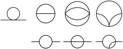
Figure 1: Topologies of relevant Feynman diagrams. The upper row represents vacuum diagrams ordered by number of loops and propagators; each of these diagrams is the vacuum closure of the corresponding diagram at the bottom row.

In this paper we study a 3-loop 5-propagator vacuum diagram shown in Figure 2(a). We did not find a standard term for it in the literature so we felt free to refer to it as the vacuum seagull diagram, and the reason is illustrated in Figure 2. Referring to the contraction order, this diagram can be contracted to two types of diagrams: contracting edge 2 (or equivalently 3, 4 or 5) factorizes into the diameter times the tadpole and hence is known, while contracting edge 1 results in a 2-vertex 4-propagator “watermelon” diagram which we chose to leave for future study, since the associated sunset diagram is known to involve elliptic dilogarithms (in 2d), see sunset and references therein.

As usual the complexity of the integral increases with the number of non-zero mass scales. 3-loop vacuum integrals with one mass scale have been solved, and in some special cases two scales are also known analytically (see references within Freitas:2016zmy ; Martin:2016bgz ). In particular Davydychev:2000na considered the vacuum seagull in an $\epsilon$ expansion around $d=4$ with one mass scale; two arbitrary mass scales were studied in Chung:2002vp ; Kalmykov:2005hb in an $\epsilon$ expansion. Freitas:2016zmy ; Bauberger:2017nct studied this diagram with general masses in an $\epsilon$ expansion and used dispersion relations to reduce the computation to a one dimensional integral suitable for numerical integration. Martin:2016bgz studied the vacuum seagull around $d=4$ by using the method of differential equations (essentially the same as SFI) and introduced a computer package which solves an associated set of ordinary differential equations.

In the widely used Integration By Parts (IBP) method Chetyrkin:1981qh Feynman Integrals are first reduced to master integrals (MIs). The perspective of the SFI method is somewhat different: in IBP we wish to express integrals with all possible indices as a linear combination of the MIs, while in SFI we can obtain higher indices through differentiation of the general expression with respect to parameters, namely using it as a generating function. In fact, at generic points in parameter space the vacuum seagull (having all indices equal to unity) is a master integral itself, while the other master integrals correspond to simpler diagrams (contractions of the vacuum seagull), see Martin:2016bgz . At some special locus of points in parameter space the vacuum seagull can be expressed as a combination of simpler diagrams (see Section 4) and hence it is not an MI over there.

This paper is organized as follows. We start by reviewing the SFI method in Section 2. In Section 3 we apply the method to the vacuum seagull diagram and determine the SFI group $G$, the SFI equation set and the group structure. The $G$-orbits are found to be co-dimension zero, and hence the SFI method reduces the dependence on all mass parameters to a line integral over simpler diagrams. The algebraic locus is a subvariety of the parameter space where the differential SFI equation set degenerates and becomes algebraic and hence the integral can be written as a linear combination of simpler diagrams. In Section 4 we determine the algebraic locus and the solutions on it. In Section 5 we solve the SFI equation set in terms of an explicit line integral. So far the discussion applies to the most general masses. In Section 5.1 we focus our attention to a specific 3 mass scale subspace in parameter space where the source functions (integrals associated with simpler diagrams) are known explicitly in terms of special functions. In this case we are able to present a formula in terms of a 1 dimensional integral and moreover we are able to solve it explicitly in terms of (rather rare) special functions. Section 5.2 gives various checks for the results of Section 5.1. Finally in Section 6 we offer a summary of our results.

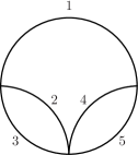
(a)

(b)

(c)

Figure 2: (a) The vacuum seagull with our labelling choice. Illustration (b) of a seagull in front of a setting sun and (c) the standard seagull vertex explain together the motivation behind the term vacuum seagull.

2 Symmetries of Feynman Integrals (SFI) method - general

Current freedom and the SFI group

Here we shall present the geometry underlying the definition of the SFI group $G$ for a general diagram, and review the derivation of the SFI system of equations. The group $G$ was defined in Kol:2015gsa and was termed “the numerator-free sub-group”. The current perspective was originally developed in the context of the vacuum seagull and was briefly introduced in Kol:2016hak , Section 2.

We start by setting the notation for a general diagram, limiting ourselves to vacuum diagrams for concreteness, though the discussion generalizes also to the presence of external legs.

Consider a general $L$ loop Feynman integral

$$I(x_{1},x_{2},\dots,x_{P},d)=\int\frac{d^{d}l_{1}\dots d^{d}l_{L}}{(k_{1}^{2}-x_{1})(k_{2}^{2}-x_{2})\dots(k_{P}^{2}-x_{P})}$$ (1)

where $x_{i}=m_{i}^{2}$ are the masses on the propagators, $\{l_{1},\dots,l_{L}\}$ are the loop momenta (or currents) and $k_{i}=C_{ir}l_{r}$ with $i=1,\dots,P$, $r=1,\dots,L$ and $C_{ir}$ a matrix of constants, are the propagator momenta. The value of this integral is invariant under invertible linear transformations of the loop momenta $\tilde{l}_{a}=L_{ab}l_{b}$ where $L_{ab}\in GL(L)$ and the SFI group $G$ is a particular subgroup of $GL(L)$ as we will see below.

Given a choice of loop currents $l_{r},r=1,\dots,L$ the space of currents is given by the span

$$C:=Sp\{l_{r}\}_{r=1}^{L}~{}.$$ (2)

Next we recall the definition of the space of potential numerators $M$ given by

$$M:=Q/S$$ (3)

where

$$Q=S^{2}(C)\equiv Sp\{l_{r}\cdot l_{s}\}_{r,s=1}^{L}$$ (4)

is the space of all quadratic Lorentz scalars made out of currents, and

$$S=Sp\{k_{i}^{2}\}_{i=1}^{P}$$ (5)

is the space of all squares, spanned by the squares of edge (or propagator) currents $k_{i},~{}i=1,\dots,P$. Since each edge current $k_{i}$ is a linear combination of loop currents, we can identify

$$S\subset Q~{}.$$ (6)

We define the SFI group $G$ as the subgroup of $GL(L)$ which preserves $S$ within $Q$ as a subspace, but not necessarily pointwise.

SFI system of equations

Now we proceed to the review of the derivation of the SFI system of equations by the current freedom perspective, which consists of viewing the the SFI equations as being generated by infinitesimal loop currents redefinitions of the form

$$l_{r}\to l_{r}+\epsilon\,l_{s}$$ (7)

for arbitrary $r,s=1,\dots,L$. This is a linear redefinition of the basis for loop currents, and as such is interpreted as the freedom to choose such a basis. For this reason we refer to the above mentioned geometric method as “current freedom”. This redefinition is the basis for both the IBP method Chetyrkin:1981qh and the method of differential equations (DE) Kotikov1a ; Kotikov1b ; Kotikov1c ; Remiddi1997 ; GehrmannRemiddi1999 . Hence we consider SFI to be a refinement of these methods. The SFI method will be applied to the vacuum seagull diagram in the next section.

The current redefinition (7) operates on the integration variables and hence leaves the integral invariant as discussed above. Any such variation translates into a recursive equation in the usual IBP set-up. However we limit ourselves to linear transformations in the subgroup $G$. This guarantees that no Lorentz scalars which are not in $S$ will be generated and hence allows to recast the recursion relation into a differential equation in $x$ space (an SFI equation). The transformation (7) induces the following transformation on the Feynman integral (1)

$$\delta I(x_{1},\dots,x_{p})=\int d^{d}l_{1}\dots d^{d}l_{L}\big{(}l_{s}\frac{\partial}{\partial l_{r}}+d\delta_{rs}\big{)}\frac{1}{(k_{1}^{2}-x_{1})(k_{2}^{2}-x_{2})\dots(k_{P}^{2}-x_{P})}~{}.$$ (8)

On the other hand the variation vanishes being a change of integration variables. This can be written as the following equation

$$\int d^{d}l_{1}\dots d^{d}l_{L}\frac{\partial}{\partial l_{r}}l_{s}\frac{1}{(k_{1}^{2}-x_{1})(k_{2}^{2}-x_{2})\dots(k_{P}^{2}-x_{P})}=0~{}.$$ (9)

Considering only the linear transformations (7) which are in $G$ we find the relevant operations $\frac{\partial}{\partial l_{r}}l_{s}$ to act on the Feynman integral. For each of these operators we get a PDE in parameter space from (9) as we will describe now. The left hand side of (9) gives a sum of terms: the first comes from operating by $\frac{\partial}{\partial l_{r}}$ on $l_{s}$ and gives back the original integral multiplied by $d$ when $r=s$; the other terms come from operating on the integrand by $\frac{\partial}{\partial l_{r}}$ and gives a sum of terms. In each of these terms one propagator from the edges of the loop $r$ is squared and a numerator of the form $l_{s}\frac{\partial k_{i}(l_{r})}{\partial l_{r}}$ is generated. Since we have considered only transformations from $G$ we can express the numerator in terms of propagators and linear combinations of $x$’s. A squared propagator $i$ in the denominator is interpreted as taking a derivative by $x_{i}$, that is, $\frac{1}{(k_{i}^{2}-x_{i})^{2}}=\frac{\partial}{\partial x_{i}}\frac{1}{(k_{i}^{2}-x_{i})}$. In this way we obtain three types of terms from equation (9): the first are constants multiplying the original integral $I(x)$, the second are linear combinations of $x$ derivatives of $I(x)$ with linear combinations of $x$ as coefficients, the third are degenerate integrals where one propagator is eliminated and another is squared; we call these integrals “sources” and denote them by $J(x)$. By doing this for each operator in $G$ we get a system of PDEs of the form

$$c_{a}\,I(x)-M_{ai}(x)\frac{\partial}{\partial x_{i}}I(x)=J_{a}(x)$$ (10)

where $a$ enumerates the equations and $i=1,\dots,P$. The matrix $M(x)$ contains the linear $x$ dependent coefficients of $\frac{\partial I}{\partial x}$ and $J(x)$ denotes sums of degenerate integrals.

We believe that the SFI equation set is essentially not different from DE. SFI added value includes insisting on considering the whole set, exposing the underlying geometry (identification of $G$ and the foliation of parameter space) and finally steps towards the solution of the set (including the reduction to the line integral). In the next section we find the system of PDEs for a specific three loop vacuum diagram.

3 SFI group and system of equations for vacuum seagull

In this section we shall apply the SFI method to the vacuum seagull diagram to obtain the SFI group $G$ and the SFI equation set.

Consider the three-loop five-propagator diagram shown in Figure 2(a). For general masses on the propagator legs this diagram is given by the following integral

$$I(x_{1},\dots,x_{5},d) = \int\frac{d^{d}l_{1}d^{d}l_{2}d^{d}l_{3}}{(l_{1}^{2}-x_{1})(l_{2}^{2}-x_{2})((l_{1}+l_{2})^{2}-x_{3})(l_{3}^{2}-x_{4})((l_{1}+l_{3})^{2}-x_{5})}$$ (11)

where $x_{i}\equiv m_{i}^{2}$. The value of the integral depends only on the parameter space

$$X:=\{x_{i}\}_{i=1}^{5}$$ (12)

and on the spacetime dimension $d$.

SFI group for vacuum seagull

Let us apply the geometrical procedure from the previous section. The vacuum seagull has 3 loops ($L=3$) and hence $\rm{dim}(Q)=6$ while the number of propagators is 5, or equivalently $\rm{dim}(S)=5$. Therefore $\rm{dim}(M)=\rm{dim}(Q)-\rm{dim}(S)=1$. In all previously studies cases (the diameter and the bubbled diagrams) there were no potential numerators (namely $\rm{dim}(M)=0$) and so this is our first example with (non-trivial) potential numerators.

We shall see here how the current freedom perspective can facilitate the determination of the group $G$ for the diagram under study. According to the conventions of (11) the square subspace is given by

$$S=Sp\{l_{1}^{2},\,l_{2}^{2},\,l_{3}^{2},\left(l_{1}+l_{2}\right)^{2},\,\left(l_{1}+l_{3}\right)^{2}\,\}~{}.$$ (13)

Since $S$ is a 5-dimensional subspace of a 6d space, it is more convenient to characterize it by its perpendicular subspace $S_{\perp}$, which is a subspace of $Q^{*}$, the dual of $Q$. More concretely, the space dual the space of loop currents $C$ is spanned by ${\partial}^{r}\equiv{\partial}/{\partial}l_{r},~{}r=1,2,3$, and accordingly

$$Q^{*}=Sp\{{\partial}^{r}\cdot{\partial}^{s}\}_{r,s=1}^{3}~{}.$$ (14)

Since $s_{\perp}:={\partial}^{2}{\partial}^{3}$ annihilates all generators of $S$ (13) one sees that

$$S_{\perp}:=Sp\{{\partial}^{2}{\partial}^{3}\}~{}.$$ (15)

Transformations which preserve the 1d subspace $S_{\perp}$ must rescale $s_{\perp}$, and hence $G$ can be decomposed as

$$G=\{r\,\mathbb{1}\}\times G_{1}$$ (16)

where the first factor is proportional to the unit matrix $\mathbb{1}$ and $G_{1}$ is defined to preserve $s_{\perp}$. Since $s_{\perp}$ is a quadratic form of signature $(+-0)$, $G_{1}$ can be identified with a Lorentz group of a degenerate 3d space (with one timelike direction, one spacelike and one null). Concretely $G_{1}$ is seen to consist of transformations of the form

$$\left[\begin{array}[]{ccc}{\partial}^{1}&{\partial}^{2}&{\partial}^{3}\end{array}\right]=\left[\begin{array}[]{ccc}{\partial}^{\prime 1}&{\partial}^{\prime 2}&{\partial}^{\prime 3}\end{array}\right]\left[\begin{array}[]{ccc}a&0&0\\ &e^{w}&0\\ &0&e^{-w}\end{array}\right]$$ (17)

where $a\neq 0$ so that the transformation is invertible and $*$ denotes an arbitrary entry, independent of all other $*$s. After allowing back the unit matrix we find that $G$ is generated by the transformations

$$\left[\begin{array}[]{ccc}{\partial}^{1}&{\partial}^{2}&{\partial}^{3}\end{array}\right]=\left[\begin{array}[]{ccc}{\partial}^{\prime 1}&{\partial}^{\prime 2}&{\partial}^{\prime 3}\end{array}\right]\left[\begin{array}[]{ccc}*&0&0\\ &*&0\\ &0&*\end{array}\right]$$ (18)

(as long as the diagonal entries are non-zero).

This action translates back to generators in $C$ space as

$$\delta\left[\begin{array}[]{c}l_{1}\\ l_{2}\\ l_{3}\end{array}\right]=\left[\begin{array}[]{ccc}*&0&0\\ &*&0\\ &0&*\end{array}\right]\left[\begin{array}[]{c}l_{1}\\ l_{2}\\ l_{3}\end{array}\right]$$ (19)

where now the $*$’s are completely unconstrained. This can be seen as follows. A linear transformation of the form ${\partial}^{r}={\partial}^{\prime s}M_{s}^{~{}r}$ implies that $M_{s}^{~{}r}={\partial}l^{\prime}_{s}/{\partial}l_{r}$ and hence $l_{r}=(M^{-1})_{r}^{~{}s}\,l^{\prime}_{s}$. Given a linear transformation of form (18) both its inverse and the associated generators have a similar form leading to (19).

The form of the generators given by (19) means that $G$ has 5 generators, namely $\rm{dim}(G)=5$, and they can be listed as follows $\frac{{\partial}}{{\partial}l_{1}}l_{1},\,\frac{{\partial}}{{\partial}l_{2}}l_{2},\,\frac{{\partial}}{{\partial}l_{2}}l_{1},\,\frac{{\partial}}{{\partial}l_{3}}l_{3},\,\frac{{\partial}}{{\partial}l_{3}}l_{1}$. Note that while both $\rm{dim}(G)$ and the number of propagators happen to be 5 for the vacuum seagull, this property is a coincidence and does not generalize to other diagrams.

SFI system of equations for vacuum seagull

Applying these $5$ generators to (11) results in 5 linear PDEs which are of the form

$$c_{a}I(x)-M_{ai}(x)\,\frac{\partial}{\partial x_{i}}I(x)=J_{a}(x)$$ (20a)

where $$a=1,\dots,5 i=1,\dots,5 c_{a} d M(x) 5\times 5 x J_{a}(x) I(x)$$ enumerates the equations and is the propagator index. are constants that can depend on ; is a matrix with entries linear in and are combinations of integrals which originate from by eliminating one propagator and squaring another. Their explicit forms are given by

$$c=\begin{pmatrix}d-4\\ d-3\\ 0\\ d-3\\ 0\end{pmatrix},\quad J(x)=\begin{pmatrix}J_{13}-J_{23}+J_{15}-J_{45}\\ -J_{13}+J_{23}\\ -J_{12}+J_{32}+J_{13}-J_{23}\\ -J_{15}+J_{45}\\ -J_{14}+J_{54}+J_{15}-J_{45}\end{pmatrix}$$ (20b)

$$M(x)=\begin{pmatrix}2x_{1}&0&x_{1}-x_{2}+x_{3}&0&x_{1}-x_{4}+x_{5}\\ 0&2x_{2}&-x_{1}+x_{2}+x_{3}&0&0\\ 0&-x_{1}-x_{2}+x_{3}&x_{1}-x_{2}+x_{3}&0&0\\ 0&0&0&2x_{4}&-x_{1}+x_{4}+x_{5}\\ 0&0&0&-x_{1}-x_{4}+x_{5}&x_{1}-x_{4}+x_{5}\end{pmatrix}$$ (20c)

where $J_{ij}$ are the integrals obtained from Equation (11) by contracting the propagator $i$ and squaring the propagator $j$; their explicit form is given in (61)-(68).

The topologies of the $J$ integrals are given by the two possible degenerations of $I(x)$:

$$\mathrm{Degen}\left[\raisebox{-12.0pt}{\includegraphics[scale={0.2}]{3loop5prop}}\right]=\left\{\raisebox{-12.0pt}{\includegraphics[scale={0.2}]{3loop_4prop_vacuum}}\,,\;\raisebox{-7.0pt}{\includegraphics[scale={0.2}]{tadpole_w_ex}}\times\raisebox{-9.0pt}{\includegraphics[scale={0.2}]{2loop_3prop}}\right\}.$$

Group orbits within parameter space

The set of differential equations (20) defines the differential operators

$$T_{a}(x)\equiv M_{ai}(x)\frac{\partial}{\partial x_{i}},\quad a=1,\dots,5$$ (21)

which form a representation of $G$ on the parameter space $X$.

Computing the determinant $\det[M(x)]$ (see (24) below) we find that at a generic point in the 5 dimensional $X$ space the 5 operators $T_{a}$ are linearly independent, and hence the generic orbit is 5 dimensional, or in other words

$$\mathrm{codim}(G\,\mathrm{orbits})=0~{}.$$ (22)

This statement tells us that it is enough to know the value of the integral at a specific point (or at most at a discrete set) and then perform a line integral to any desired point in $X$ space. In the next section we will discuss special hypersurfaces which we call “the algebraic locus” on which the set $\{T_{a}\}$ is degenerate and where we can find algebraic solutions for $I(x)$ in terms of $J_{a}(x)$.

The $T_{a}$ operators (21) inherit the group structure of the fundamental set of operators $\frac{{\partial}}{{\partial}l_{1}}l_{1},\,\frac{{\partial}}{{\partial}l_{2}}l_{2},\,\frac{{\partial}}{{\partial}l_{2}}l_{1},\,\frac{{\partial}}{{\partial}l_{3}}l_{3},\,\frac{{\partial}}{{\partial}l_{3}}l_{1}$. In particular we find that they satisfy the commutation relations

$$[T_{3},T_{2}]=T_{3},\quad[T_{5},T_{4}]=T_{5}~{}.$$ (23)

The operator $T_{1}+T_{2}+T_{4}$ is responsible for transformations in the radial direction in $X$ space (the dimension operator). Using this observation and the commutation relations (23) we find that our group decomposes as $G=U(1)_{\mathrm{radial}}\times U(1)^{2}\rtimes U(1)^{2}$.

4 Algebraic locus

Before proceeding to the solution of the SFI system of equations (20), it is worth discussing a special set of hypersurfaces within the parameter space on which the system is degenerate and the value of the integral is determined algebraically.

For this diagram the matrix $M_{ai}(x)$ defined in (20c) is square and therefore we can compute its determinant

$$\det[M(x)]=-2x_{1}\lambda(x_{1},x_{2},x_{3})\lambda(x_{1},x_{4},x_{5})$$ (24)

where

$$\lambda(x,y,z)=x^{2}+y^{2}+z^{2}-2xy-2xz-2yz$$ (25)

is the Heron or Källén invariant. Since $\det[M(x)]\neq 0$ generically, we see that generic $G$ orbits are 5 dimensional. Furthermore, we see that the set $\{T_{a}\}$ is degenerate on the following hypersurfaces in $X$ space:

$$x_{1} = 0$$ (26)

$$\lambda_{123}\equiv\lambda(x_{1},x_{2},x_{3}) = 0$$ (27)

$$\lambda_{145}\equiv\lambda(x_{1},x_{4},x_{5}) = 0~{}.$$ (28)

As we shall explain immediately below, (20) reduces to algebraic equations for $I(x)$ on these hypersurfaces, therefore we will refer to them as “algebraic locus” hypersurfaces. They are represented schematically in Figure 3.

Figure 3: Schematic projective representation of $X$ space: the circle in the left triangle is $\lambda(x_{1},x_{2},x_{3})=0$, the circle in the right triangle is $\lambda(x_{1},x_{4},x_{5})=0$ and $x_{1}=0$ is represented by $(x_{2}x_{3})\cup(x_{4}x_{5})$.

Let us multiply (20) by the matrix of polynomials $\tilde{M}(x):=\text{det}[M(x)]M^{-1}(x)$

$$\tilde{M}(x)_{ia}c_{a}I-\text{det}[M(x)]\partial_{i}I=\tilde{M}(x)_{ia}J_{a}~{}.$$ (29)

Setting $\text{det}[M(x)]=0$ we arrive at a system of algebraic equations for $I(x)$:

$$(d-3)\begin{pmatrix}x_{145}x_{154}\lambda_{123}+x_{123}x_{132}\lambda_{145}-\frac{d-4}{d-3}\lambda_{123}\lambda_{145}\\ -2x_{1}x_{132}\lambda_{145}\\ -2x_{1}x_{123}\lambda_{145}\\ -2x_{1}x_{154}\lambda_{123}\\ -2x_{1}x_{145}\lambda_{123}\end{pmatrix}I$$ (30)

$$\quad=\begin{pmatrix}\lambda_{123}[2x_{5}x_{145}(J_{45}-J_{15})+2x_{4}x_{154}(J_{54}-J_{14})]+(4,5)\leftrightarrow(2,3)\\ -2x_{1}x_{231}\lambda_{145}(J_{12}-J_{32})+4x_{1}x_{3}\lambda_{145}(J_{13}-J_{23})\\ -2x_{1}x_{321}\lambda_{145}(J_{13}-J_{23})+4x_{1}x_{2}\lambda_{145}(J_{12}-J_{32})\\ -2x_{1}x_{451}\lambda_{123}(J_{14}-J_{54})+4x_{1}x_{5}\lambda_{123}(J_{15}-J_{45})\\ -2x_{1}x_{541}\lambda_{123}(J_{15}-J_{45})+4x_{1}x_{4}\lambda_{123}(J_{14}-J_{54})\end{pmatrix}$$

where we have defined $x_{ijk}:=x_{i}-x_{j}-x_{k}$. Now we can analyze the solutions of these equations on each branch of the algebraic locus (26-28) separately.

Solutions on $x_{1}=0$. To find the algebraic solution on $x_{1}=0$ we simply set $x_{1}=0$ in (30) to get

$$(d-2)I(0,x_{2},x_{3},x_{4},x_{5}) = \frac{2x_{2}\big{(}J_{32}-J_{12}\big{)}-2x_{3}\big{(}J_{23}-J_{13}\big{)}}{x_{2}-x_{3}}$$ (31)

$$+\frac{2x_{4}\big{(}J_{54}-J_{14}\big{)}-2x_{5}\big{(}J_{45}-J_{15}\big{)}}{x_{4}-x_{5}}~{}.$$

From here we can examine several simpler cases. For example, when additionally $x_{3}=x_{5}=0$ we get

$$(d-2)I(0,x_{2},0,x_{4},0)=2(J_{32}-J_{12})+2(J_{54}-J_{14})~{}.$$ (32)

We confirm that this result coincides with the answer obtained via FIRE Smirnov:2014hma .

Solutions on $\lambda_{123}=0$ and $\lambda_{145}=0$. On $\lambda_{145}=0$ we can find the solution for $I(x)$ by setting $\lambda_{145}=0$ in (30). Note that adding to the solution a multiple of $\lambda_{145}$ does not change the value of $I(x)$ and therefore we can get different but equivalent expressions for $I(x)$ on the algebraic locus hypersurfaces. The nicest form for the expression we got is

$$(d-3)I(x)=\sqrt{\frac{x_{4}}{x_{1}}}(J_{54}-J_{14})+\sqrt{\frac{x_{5}}{x_{1}}}(J_{45}-J_{15})~{}.$$ (33)

The solution on $\lambda_{123}=0$ can be read from (33) by exchanging $(4,5)\leftrightarrow(2,3)$. We also have compared this solution with the answer of FIRE for the point $x_{1}=x_{4}=m^{2}$, $x_{3}=x_{5}=0$ and $x_{2}=M^{2}$ and found full agreement.

An alternative combined expression on $\det[M(x)]=0$. From (30) a general solution for $I(x)$ on the algebraic locus can be obtained

$$I(x)=-\frac{2\big{[}\big{(}x_{1}(x_{1}-x_{3})+x_{2}(x_{2}-x_{3})\big{)}(J_{12}-J_{32})+(2\leftrightarrow 3)\big{]}\lambda_{145}+(2,3)\leftrightarrow(4,5)}{(d-3)(3x_{1}^{2}+(x_{2}-x_{3})^{2})\lambda_{145}+(2,3)\leftrightarrow(4,5)-(d-4)\lambda_{123}\lambda_{145}}~{}.$$ (34)

From this general expression one can read off the solutions (31) and (33) as well as solutions on intersections of the algebraic locus hypersurfaces.

5 Solution

It is always possible to reduce the solution to the SFI equation set into a line integral Kol:2015gsa . Here we apply this general procedure to (20). In the next section we will perform the line integral for a 3 dimensional parameter space.

The homogeneous solution of (20) is

$$I_{0}(x)=x_{1}^{1-\frac{d}{2}}\left[\lambda(x_{1},x_{2},x_{3})\lambda(x_{1},x_{4},x_{5})\right]^{\frac{d-3}{2}}~{}.$$ (35)

The complete solution could be presented in the following form

$$I(x)=I_{0}(x)c(x)$$ (36)

where $c(x)$ should satisfy

$$\begin{pmatrix}{\partial}_{x_{1}}\\ {\partial}_{x_{2}}\\ {\partial}_{x_{3}}\\ {\partial}_{x_{4}}\\ {\partial}_{x_{5}}\end{pmatrix}c(x)=\frac{1}{I_{0}(x)}\begin{pmatrix}\frac{\lambda_{123}\lambda_{145}J_{1}-\{(x_{1}-x_{2}+x_{3})\lambda_{145}\big{(}(x_{1}+x_{2}-x_{3})J_{2}+2x_{2}J_{3}\big{)}+(2,3)\leftrightarrow(4,5)\}}{2x_{1}\lambda_{123}\lambda_{145}}\\ \frac{(x_{1}-x_{2})(J_{2}+J_{3})+x_{3}(J_{2}-J_{3})}{\lambda_{123}}\\ \frac{2x_{2}J_{3}+(x_{1}+x_{2}-x_{3})J_{2}}{\lambda_{123}}\\ \frac{(x_{1}-x_{4})(J_{4}+J_{5})+x_{5}(J_{4}-J_{5})}{\lambda_{145}}\\ \frac{2x_{4}J_{5}+(x_{1}+x_{4}-x_{5})J_{4}}{\lambda_{145}}\end{pmatrix}~{}.$$ (37)

The value of $c(x)$ at any point $B$ in the parameter space can be calculated by a line integral from a chosen starting point $A$ to $B$ along an arbitrary path $\gamma$

$$c(B) = \int_{\gamma}\Big{[}\frac{\lambda_{123}\lambda_{145}J_{1}-\{(x_{1}-x_{2}+x_{3})\lambda_{145}\big{(}(x_{1}+x_{2}-x_{3})J_{2}+2x_{2}J_{3}\big{)}+(2,3)\leftrightarrow(4,5)\}}{2x_{1}\lambda_{123}\lambda_{145}I_{0}}dx_{1}$$ (38)

$$+\frac{(x_{1}-x_{2})(J_{2}+J_{3})+x_{3}(J_{2}-J_{3})}{\lambda_{123}I_{0}}dx_{2}+\frac{2x_{2}J_{3}+(x_{1}+x_{2}-x_{3})J_{2}}{\lambda_{123}I_{0}}dx_{3}$$

$$+\frac{(x_{1}-x_{4})(J_{4}+J_{5})+x_{5}(J_{4}-J_{5})}{\lambda_{145}I_{0}}dx_{4}+\frac{2x_{4}J_{5}+(x_{1}+x_{4}-x_{5})J_{4}}{\lambda_{145}I_{0}}dx_{5}\Big{]}+c(A)~{}.$$

From (36) it follows that

$$c(A)=\frac{I(A)}{I_{0}(A)}$$ (39)

it is therefore useful to choose the starting point $A$ where $I(A)$ is easy to calculate by other methods (for example where all but one of the masses are zero). Given (38) the complete solution at any point $B$ is given by

$$I(B)=I_{0}(B)c(B)~{}.$$ (40)

Now we shall present a concrete form for $I(B)$ by choosing a starting point $A$ and a path $\gamma$ from $A$ to a general point $B$ in $X$ space. We choose $A$ to be the point where $x_{1}=m^{2}$ and all the rest of the masses are zero, and $\gamma$ to be a straight line with constant $x_{1}$ such that

$$A = m^{2}(1,0,0,0,0)$$ (41a)

$$B = m^{2}(1,x,u,y,v)$$ (41b)

and it is parameterized by

$$(x_{1}(t),x_{2}(t),x_{3}(t),x_{4}(t),x_{5}(t))=m^{2}(1,x\,t,u\,t,y\,t,v\,t),\quad 0\leq t\leq 1~{}.$$ (41c)

Along this path $dx_{1}=0$ and the first term in (38) vanishes. We can therefore write

$$I(B) = \big{(}\lambda(1,x,u)\lambda(1,y,v)\big{)}^{\frac{d-3}{2}}$$ (42)

$$\times \Bigg{\{}\int_{0}^{1}\left[\lambda(1,xt,ut)\lambda(1,yt,vt)\right]^{\frac{3-d}{2}}$$

$$\Big{[}\frac{x(1-xt)(-J_{12}+J_{32})+u(1-ut)(-J_{13}+J_{23})+xut(-J_{12}+J_{32}-J_{13}+J_{23})}{\lambda(1,xt,ut)}$$

$$+\frac{y(1-yt)(-J_{14}+J_{54})+v(1-vt)(-J_{15}+J_{45})+yvt(-J_{14}+J_{54}-J_{15}+J_{45})}{\lambda(1,yt,vt)}\Big{]}dt$$

$$+\frac{I(m^{2},0,0,0,0)}{(m^{2})^{3d/2-5}}\Bigg{\}}~{}.$$

Note that the 2 terms in the integrand are related by symmetry, and that the $m^{2}$ dependence comes from the sources. In the next section we compute this integral on a reduced parameter space where $x_{3}=x_{5}=0$.

5.1 Solution with 3 different mass scales

On the subspace with $x_{3}=x_{5}=0$ all of the sources $J_{ij}$ are known in terms of special functions and we can perform the 1-dimensional integral (42) to get $I(x_{1},x_{2},0,x_{4},0)$ in terms of special functions as we will explain below. This 3 dimensional subspace $(x_{1},x_{2},x_{4})$ is depicted in Figure 4 where the blue lines represent the algebraic locus surfaces $x_{1}=0$, $x_{1}=x_{2}$ and $x_{1}=x_{4}$ and the thick black line represents the path (41) with $x_{3}=x_{5}=0$.

Figure 4: Projective representation of the 3 dimensional parameter space $(x_{1},x_{2},x_{4})$, namely the subspace $x_{1}+x_{2}+x_{4}=m^{2}$. The blue lines represent the algebraic locus surfaces. The thick line represents the trajectory from $A=m^{2}(1,0,0)$ to $B=m^{2}(1,x,y)$ with parameterization $(x_{1}(t),x_{2}(t),x_{4}(t))=m^{2}(1,x\,t,y\,t)$ and $0\leq t\leq 1$. The red shaded kite represents the region where the solution (50) is manifestly non-singular.

Setting $x_{3}=x_{5}=0$ (equivalently $u=v=0$) into (42) we get the following integral

$$I(m^{2},m^{2}x,0,m^{2}y,0) = \left[(1-x)(1-y)\right]^{d-3}\Big{\{}\int_{0}^{1}\Big{[}\frac{x(-J_{12}+J_{32})}{(1-xt)^{d-2}(1-yt)^{d-3}}$$

$$+\frac{y(-J_{14}+J_{54})}{(1-yt)^{d-2}(1-xt)^{d-3}}\Big{]}dt+\frac{I(m^{2},0,0,0,0)}{(m^{2})^{3d/2-5}}\Big{\}}~{}.$$

The expressions for $J_{12}$, $J_{14}$, $J_{32}$ and $J_{54}$ with $x_{3}=x_{5}=0$ are given by (71-74). On the chosen trajectory (41) they have the form

$$J_{12}(t) = -e^{-\frac{3}{2}(d-4)\gamma_{E}}(m^{2})^{\frac{3d}{2}-5}(y\,t)^{\frac{3d}{2}-5}\frac{\big{(}\Gamma(d/2-1)\big{)}^{2}}{\Gamma(d/2)}$$ (43)

$$\times \Big{[}\Gamma\big{(}5-\frac{3d}{2}\big{)}\Gamma(4-d)\Gamma\big{(}\frac{d}{2}-2\big{)}{{}_{2}F_{1}}\big{(}5-\frac{3d}{2},4-d,3-\frac{d}{2}\big{|}\frac{x}{y}\big{)}$$

$$+ \Big{(}\frac{x}{y}\Big{)}^{d/2-2}\Gamma(3-d)\big{(}\Gamma(2-d/2)\big{)}^{2}{{}_{2}F_{1}}\big{(}3-d,2-\frac{d}{2},\frac{d}{2}-1\big{|}\frac{x}{y}\big{)}\Big{]}$$

$$J_{32}(t) = -e^{-\frac{3}{2}(d-4)\gamma_{E}}(m^{2})^{\frac{3d}{2}-5}(x\,t)^{\frac{d}{2}-2}\frac{\Gamma(2-d/2)}{\Gamma(d/2)}$$ (44)

$$\times \Big{[}\Gamma(3-d)\Gamma\big{(}2-\frac{d}{2}\big{)}\big{(}\Gamma\big{(}\frac{d}{2}-1\big{)}\big{)}^{2}(1-y\,t)^{d-3}$$

$$+ (y\,t)^{\frac{d}{2}-1}\Gamma\big{(}1-\frac{d}{2}\big{)}\Gamma\big{(}2-\frac{d}{2}\big{)}\Gamma\big{(}\frac{d}{2}-1\big{)}{{}_{2}F_{1}}\big{(}1,2-\frac{d}{2},\frac{d}{2}\big{|}y\,t\big{)}\Big{]}~{}.$$

$J_{14}(t)$ and $J_{54}(t)$ are obtained from (43) and (44) respectively by $x\leftrightarrow y$. At the starting point $A$ the value of the integral is easily calculated to be

$$I(m^{2},0,0,0,0)=-e^{-\frac{3}{2}(d-4)\gamma_{E}}(m^{2})^{\frac{3d}{2}-5}\frac{\Gamma(5-3d/2)(\Gamma(2-d/2))^{2}(\Gamma(d/2-1))^{4}\Gamma(3d/2-4)}{(\Gamma(d-2))^{2}\Gamma(d/2)}~{}.$$ (45)

Plugging the explicit expressions (43), (44) into (5.1) we organize the result according to the different $t$ integrals to be performed:

$$I(m^{2},m^{2}x,0,m^{2}y,0) = (m^{2})^{\frac{3d}{2}-5}\big{(}(1-x)(1-y)\big{)}^{d-3}$$ (46a)

$$\Big{\{}c_{1}(x,y,d)\int_{0}^{1}\frac{t^{\frac{3d}{2}-5}}{(1-x\,t)^{d-2}(1-y\,t)^{d-3}}dt$$

$$+c_{2}(x,y,d)\int_{0}^{1}\frac{t^{\frac{d}{2}-2}}{(1-x\,t)^{d-2}}dt$$

$$+c_{3}(x,y,d)\int_{0}^{1}\frac{t^{d-3}{{}_{2}F_{1}}\big{(}1,2-\frac{d}{2},\frac{d}{2}\big{|}y\,t\big{)}}{(1-x\,t)^{d-2}(1-y\,t)^{d-3}}dt$$

$$+x\leftrightarrow y+c_{4}(d)\Big{\}}$$

where

$$c_{1}(x,y,d) = e^{-\frac{3}{2}(d-4)\gamma_{E}}\frac{\big{(}\Gamma(d/2-1)\big{)}^{2}}{\Gamma(d/2)}\Big{[}\Gamma\big{(}5-\frac{3d}{2}\big{)}\Gamma(4-d)\Gamma\big{(}\frac{d}{2}-2\big{)}{{}_{2}F_{1}}\big{(}5-\frac{3d}{2},4-d,3-\frac{d}{2}\big{|}\frac{x}{y}\big{)}$$ (46b)

$$+\Big{(}\frac{x}{y}\Big{)}^{d/2-2}\Gamma(3-d)\big{(}\Gamma(2-d/2)\big{)}^{2}{{}_{2}F_{1}}\big{(}3-d,2-\frac{d}{2},\frac{d}{2}-1\big{|}\frac{x}{y}\big{)}\Big{]}x\,y^{\frac{3d}{2}-5}$$

$$c_{2}(x,y,d) = -e^{-\frac{3}{2}(d-4)\gamma_{E}}\frac{\Gamma(3-d)\big{(}\Gamma\big{(}2-\frac{d}{2}\big{)}\Gamma\big{(}\frac{d}{2}-1\big{)}\big{)}^{2}}{\Gamma(d/2)}\,x^{\frac{d}{2}-1}$$ (46c)

$$c_{3}(x,y,d) = -e^{-\frac{3}{2}(d-4)\gamma_{E}}\frac{\Gamma\big{(}1-\frac{d}{2}\big{)}\big{(}\Gamma\big{(}2-\frac{d}{2}\big{)}\big{)}^{2}\Gamma\big{(}\frac{d}{2}-1\big{)}}{\Gamma(d/2)}(x\,y)^{\frac{d}{2}-1}$$ (46d)

$$c_{4}(d) = -e^{-\frac{3}{2}(d-4)\gamma_{E}}\frac{\Gamma(5-3d/2)(\Gamma(2-d/2))^{2}(\Gamma(d/2-1))^{4}\Gamma(3d/2-4)}{\Gamma(d/2)(\Gamma(d-2))^{2}}~{}.$$ (46e)

The first two integrals in (46a) are recognized as the Appell $F_{1}$ function and the hypergeometric ${{}_{2}F_{1}}$

$$\int_{0}^{1}\frac{t^{\frac{3d}{2}-5}}{(1-x\,t)^{d-2}(1-y\,t)^{d-3}}dt = \frac{2}{3d-8}F_{1}(3d/2-4,d-2,d-3,3d/2-3|\,x,y)$$ (47)

$$\int_{0}^{1}\frac{t^{\frac{d}{2}-2}}{(1-x\,t)^{d-2}}dt = \frac{2}{d-2}{{}_{2}F_{1}}(d/2-1,d-2,d/2\big{|}\,x)~{}.$$ (48)

The third integral in (46a) we find to be the Kampé de Fériet function defined in (78)

$$\int_{0}^{1}\frac{t^{d-3}{{}_{2}F_{1}}\big{(}1,2-\frac{d}{2},\frac{d}{2}\big{|}y\,t\big{)}}{(1-x\,t)^{d-2}(1-y\,t)^{d-3}}dt=\int_{0}^{1}\frac{t^{d-3}{{}_{2}F_{1}}\big{(}\frac{d}{2}-1,d-2,\frac{d}{2}\big{|}y\,t\big{)}}{(1-x\,t)^{d-2}}dt$$

$$=\frac{1}{d-2}\sum_{k=0}^{\infty}\sum_{n=0}^{\infty}\frac{(d-2)_{k+n}(d-2)_{k}(d/2-1)_{n}(d-2)_{n}}{(d-1)_{k+n}(d/2)_{n}}\frac{x^{k}}{k!}\frac{y^{n}}{n!}$$

$$=\frac{1}{d-2}F^{\begin{subarray}{c}1:1;2\\ 1:0;1\end{subarray}}\left(\begin{matrix}d-2:d-2;d/2-1,d-2\\ d-1:\quad;d/2\end{matrix}\Big{|}x,y\right)~{}.$$ (49)

We thus obtain an explicit expression for the vacuum seagull diagram on the reduced parameter space with 3 arbitrary masses:

$$I(m^{2},m^{2}x,0,m^{2}y,0) = e^{-\frac{3}{2}(d-4)\gamma_{E}}(m^{2})^{\frac{3d}{2}-5}\big{(}(1-x)(1-y)\big{)}^{d-3}$$ (50)

$$\Big{\{}c_{1}(x,y,d)\frac{2}{3d-8}F_{1}(3d/2-4,d-2,d-3,3d/2-3|\,x,y)$$

$$+c_{2}(x,y,d)\frac{2}{d-2}{{}_{2}F_{1}}(d/2-1,d-2,d/2|\,x)$$

$$+c_{3}(x,y,d)\frac{1}{d-2}F^{\begin{subarray}{c}1:1;2\\ 1:0;1\end{subarray}}\left(\begin{matrix}d-2:d-2;d/2-1,d-2\\ d-1:\quad;d/2\end{matrix}\Big{|}x,y\right)$$

$$+x\leftrightarrow y+c_{4}(d)\Big{\}}~{}.$$

where all symbols were defined above. This expression is manifestly non-singular when $0<x,y<1$, namely when the end point $B$ is within the red shaded region in Figure 4.

5.2 Checks

Comparison for $x_{2}=0$

Setting $x_{2}=0$ (equivalently $x=0$) in our reduced line integral (5.1), we obtain the following integral to compute

$$I(m^{2},0,0,m^{2}y,0) = (1-y)^{d-3}\Big{\{}\int_{0}^{1}\frac{y(-J_{14}+J_{54})}{(1-yt)^{d-2}(1-xt)^{d-3}}dt+\frac{I(m^{2},0,0,0,0)}{(m^{2})^{3d/2-5}}\Big{\}}~{}.$$

The trajectory (41) for $x_{2}=0$ on the 3 dimensional subspace $(x_{1},x_{2},x_{4})$ is shown in Figure 5.

Figure 5: In the 3 dimensional parameter space $(x_{1},x_{2},x_{4})$ the thick line represents the trajectory from $A=m^{2}(1,0,0)$ to $B=m^{2}(1,0,y)$ with the parameterization $(x_{1}(t),x_{2}(t),x_{4}(t))=m^{2}(1,0,y\,t)$ and $0\leq t\leq 1$.

In this case ($x_{2}=x_{3}=x_{5}=0$) the sources $J_{14}$ and $J_{54}$ can be calculated directly from their integral definitions (63) and (68). On the trajectory given by (41) they have the following form

$$J_{14}(t) = -e^{-\frac{3}{2}(d-4)\gamma_{E}}(m^{2})^{\frac{3d}{2}-5}\frac{\Gamma(5-3d/2)\Gamma(3-d)(\Gamma(d/2-1))^{3}}{\Gamma(d/2)}(y\,t)^{3d/2-5}$$ (52)

$$J_{54}(t) = -e^{-\frac{3}{2}(d-4)\gamma_{E}}(m^{2})^{\frac{3d}{2}-5}\frac{(\Gamma(2-d/2))^{2}(\Gamma(d/2-1))^{2}\Gamma(3-d)}{\Gamma(d/2)}(y\,t)^{d/2-2}~{}.$$ (53)

Plugging (52) and (53) into (5) we find

$$I(m^{2},0,0,m^{2}y,0) = -e^{-\frac{3}{2}(d-4)\gamma_{E}}(m^{2})^{\frac{3d}{2}-5}(1-y)^{d-3}$$ (54)

$$\times\Big{[}-\frac{\Gamma(5-3d/2)\Gamma(3-d)(\Gamma(d/2-1))^{3}}{\Gamma(d/2)}\int_{0}^{1}\frac{y(y\,t)^{3d/2-5}}{(1-y\,t)^{d-2}}dt$$

$$+\frac{(\Gamma(2-d/2))^{2}(\Gamma(d/2-1))^{2}\Gamma(3-d)}{\Gamma(d/2)}\int_{0}^{1}\frac{y(y\,t)^{d/2-2}}{(1-y\,t)^{d-2}}dt$$

$$+\frac{\Gamma(5-3d/2)(\Gamma(2-d/2))^{2}(\Gamma(d/2-1))^{4}\Gamma(3d/2-4)}{(\Gamma(d-2))^{2}\Gamma(d/2)}\Big{]}$$

which we easily integrate to

$$I(m^{2},0,0,m^{2}y,0) = -e^{-\frac{3}{2}(d-4)\gamma_{E}}(m^{2})^{\frac{3d}{2}-5}(1-y)^{d-3}\frac{(\Gamma(d/2-1))^{2}}{\Gamma(d/2)}$$ (55)

$$\times\Big{[}-\Gamma(3-d)\Gamma(5-3d/2)\Gamma(d/2-1)\frac{2}{3d-8}y^{3d/2-4}{{}_{2}F_{1}}\big{(}d-2,\frac{3d}{2}-4,\frac{3d}{2}-3\big{|}y\big{)}$$

$$+(\Gamma(3-d)\Gamma(2-d/2))^{2}\frac{2}{d-2}y^{d/2-1}{{}_{2}F_{1}}\big{(}\frac{d}{2}-1,d-2,\frac{d}{2}\big{|}y)$$

$$+\frac{\Gamma(5-3d/2)(\Gamma(2-d/2))^{2}(\Gamma(d/2-1))^{2}\Gamma(3d/2-4)}{(\Gamma(d-2))^{2}}\Big{]}~{}.$$

We have compared this result with direct calculation via Schwinger parameters and found complete agreement. We have also performed the line integral starting at $(x_{1},x_{2},x_{4})=m^{2}(0,0,1)$. In addition we checked that in the limit $x\to 0$ (50) reduces to (55). We note that this integral has been evaluated in closed form in Kalmykov:2011ks , Eqs. (114, 116).

Epsilon expansion

In this subsection we present the results for the $\epsilon$-expansion of the vacuum seagull diagram around critical dimension $d=4$. This could serve as another check for our line integral answer (5.1), as we will compare our results obtained from this line integral with the results of two recent papers, Freitas:2016zmy and Martin:2016bgz , and will find perfect agreement.

Within the SFI approach one just needs to know the $\epsilon$-expansion of the sources, calculate the $\epsilon$-expansion of the homogeneous solution, combine them together under the line integral and perform this last integration. The general solution for 3 mass scales (5.1) can be presented as follows

$$I(B)=\int_{0}^{1}\frac{I_{0}(B)(J_{12}-J_{32})x}{(1-xt)^{d-2}(1-yt)^{d-3}}dt+\left(x\leftrightarrow y\right)+\frac{I_{0}(B)}{I_{0}(A)}I(A)~{}.$$ (56)

We will use this expression to study the $\epsilon$-expansion. In general, the $\epsilon$-expansion for the $I(B)$ could be written as follows

$$I(B)=I_{3}(B)\epsilon^{-3}+I_{2}(B)\epsilon^{-2}+I_{1}(B)\epsilon^{-1}+I_{0}(B)~{}.$$ (57)

Here we will discuss the first two leading divergent parts.

Order $\epsilon^{-3}$. Using explicit expressions for the sources (43), (44), one finds

$$\frac{I_{0}(B)(J_{12}-J_{32})x}{(1-xt)^{d-2}(1-yt)^{d-3}} = \frac{m^{2}x(1-x)(1-y)(3+ty)}{6(1-tx)^{2}(1-ty)}\epsilon^{-3}+\mathcal{O}(\epsilon^{-2})$$

$$\frac{I_{0}(B)}{I_{0}(A)}I(A) = \frac{1}{3}m^{2}(1-x)(1-y)\epsilon^{-3}+\mathcal{O}(\epsilon^{-2})$$

performing the integral over $t$ from $0$ to $1$ and combining all terms together we arrive to the following very simple expression

$$I_{3}(B)=\frac{1}{6}m^{2}\left(2+x+y\right)=\frac{1}{6}\left(2m_{1}^{2}+m_{2}^{2}+m_{4}^{2}\right)$$ (58)

which coincide with the expressions from Freitas:2016zmy and Martin:2016bgz , after proper redefinitions and in the limit of $m_{3}=m_{5}=0$.

Order $\epsilon^{-2}$. In this case the expressions are a bit longer and there is no point to present them explicitly. Naively, dilogarithms appear at this order after integration. However, by using the following identity

$$\rm{Li}_{2}(z)+\rm{Li}_{2}(1-z)=\frac{\pi^{2}}{6}-\log{(z)}\log{(1-z)}$$ (59)

we can get rid of them and after all other possible simplifications we arrive to the following answer for the $\epsilon^{-2}$ order term

$$I_{2}(B) = \frac{m^{2}}{6}\left[10+6x+6y+3(2+x+y)\log{m^{2}}+3x\log{x}+3y\log{y}\right]=$$ (60)

$$= m_{1}^{2}\left(\frac{5}{3}-\log{m_{1}^{2}}\right)+m_{2}^{2}\left(1-\frac{1}{2}\log{m_{2}^{2}}\right)+m_{4}^{2}\left(1-\frac{1}{2}\log{m_{4}^{2}}\right)$$

which is again in an agreement with Freitas:2016zmy and Martin:2016bgz .

Numerical results

The integral (5.1) with (43) and (44) can be integrated numerically for non-integer $d$. In Table 1 we present numerical results for various values of $d$ with $x_{1}=1$ and $x_{2},x_{4}\in[0.01,0.9]$. These values of $x_{1},x_{2},x_{4}$ cover the region colored in red in Figure 4. We did not cross the algebraic locus surfaces since the integral (5.1) diverges there and must be regularized. We have compared the numerical integral values with the values obtained from our explicit analytic solution (50) and found complete agreement.

Table 1: Numerical results for various $d$. We normalized the results by setting $x_{1}=1$ and $x_{2},x_{4}\in[0.01,0.9]$. The horizontal and vertical axis represent increasing $x_{2}$ and $x_{4}$ respectively.

$d=3.2$	$d=3.7$
$d=3.8$	$d=3.9$
$d=4.1$	$d=4.2$

6 Summary

In this section we summarize our results

• We applied the SFI method to the vacuum seagull. The group $G$ is given by (19) and equivalently by the defining relations (23); the $G$ foliation is found to be co-dimension 0 (22). The SFI differential equation set is given in (20). Finally, the expression for the vacuum seagull diagram in terms of a line integral over simpler diagrams is given in (38-40). A concrete 1-dimensional realization for the line integral is given in (42).

• We presented a geometrical method to determine $G$ as the stabilizer of the space of squares inside the space of quadratics, see Section 3 as well as Kol:2016veg . We presented the first example for this method in the presence of potential numerators (the vacuum seagull has one potential numerator). This method provides the geometry underlying the definition of the group $G$ introduced in Kol:2016hak , and allows for a simplified determination of $G$.

• We obtained explicit results for an integral with 3 mass scales (in the reduced parameter space) in terms of a (rare) special function (50), or alternatively in terms of an explicit 1 dimensional integral (46). This might be the first explicit determination of a 3-loop diagram with 3 arbitrary mass scales. We also supplied numerical results over the reduced parameter space (see Table 1) and some terms in the $\epsilon$-expansion (58, 60).

This work adds to that of the closely related Martin:2016bgz not only by the last item above, but also by presenting the equation set explicitly, as well as by determining the group structure and the $G$-foliation of parameter space, thereby exposing the underlying geometry.

Acknowledgments

We are grateful to A. Davydychev, A. Freitas, S. Martin, D. Robertson and V. Smirnov for useful comments on a draft. We also thank M. Kalmykov and A. Kotikov for useful correspondence. This research was supported by the “Quantum Universe” I-CORE program of the Israel Planning and Budgeting Committee.

Appendix A Appendix

Source integrals

$J_{ij}$ are the integrals obtained from equation (11) by contracting the propagator $i$ and squaring the propagator $j$.

$$J_{12} = \int\frac{d^{d}l_{1}d^{d}l_{2}d^{d}l_{3}}{(l_{2}^{2}-x_{2})^{2}((l_{1}+l_{2})^{2}-x_{3})(l_{3}^{2}-x_{4})((l_{1}+l_{3})^{2}-x_{5})}$$ (61)

$$J_{13} = \int\frac{d^{d}l_{1}d^{d}l_{2}d^{d}l_{3}}{(l_{2}^{2}-x_{2})((l_{1}+l_{2})^{2}-x_{3})^{2}(l_{3}^{2}-x_{4})((l_{1}+l_{3})^{2}-x_{5})}$$ (62)

$$J_{14} = \int\frac{d^{d}l_{1}d^{d}l_{2}d^{d}l_{3}}{(l_{2}^{2}-x_{2})((l_{1}+l_{2})^{2}-x_{3})(l_{3}^{2}-x_{4})^{2}((l_{1}+l_{3})^{2}-x_{5})}$$ (63)

$$J_{15} = \int\frac{d^{d}l_{1}d^{d}l_{2}d^{d}l_{3}}{(l_{2}^{2}-x_{2})((l_{1}+l_{2})^{2}-x_{3})(l_{3}^{2}-x_{4})((l_{1}+l_{3})^{2}-x_{5})^{2}}$$ (64)

$$J_{23} = \int\frac{d^{d}l_{1}d^{d}l_{2}d^{d}l_{3}}{(l_{1}^{2}-x_{1})((l_{1}+l_{2})^{2}-x_{3})^{2}(l_{3}^{2}-x_{4})((l_{1}+l_{3})^{2}-x_{5})}$$ (65)

$$J_{32} = \int\frac{d^{d}l_{1}d^{d}l_{2}d^{d}l_{3}}{(l_{1}^{2}-x_{1})(l_{2}^{2}-x_{2})^{2}(l_{3}^{2}-x_{4})((l_{1}+l_{3})^{2}-x_{5})}$$ (66)

$$J_{45} = \int\frac{d^{d}l_{1}d^{d}l_{2}d^{d}l_{3}}{(l_{1}^{2}-x_{1})(l_{2}^{2}-x_{2})((l_{1}+l_{2})^{2}-x_{3})((l_{1}+l_{3})^{2}-x_{5})^{2}}$$ (67)

$$J_{54} = \int\frac{d^{d}l_{1}d^{d}l_{2}d^{d}l_{3}}{(l_{1}^{2}-x_{1})(l_{2}^{2}-x_{2})((l_{1}+l_{2})^{2}-x_{3})(l_{3}^{2}-x_{4})^{2}}~{}.$$ (68)

The integrals (61-64) are of the “watermelon” topology discussed in the introduction; these integrals and their associated “sunset” diagrams can be represented in terms of 1-dimensional integrals of Bessel functions Groote:2005ay ; Berends:1993ee ; Mendels:1978wc . The integrals (65-68) have the topology of a product of the 2-loop “diameter” diagram and a tadpole.

Expressions for sources on reduced parameter space

On the 3 dimensional subspace discussed in Section 5.1 all of the sources can be obtained from the following vacuum two loop integral (diameter topology)

$$J(n_{1},n_{2},n_{3};x_{1},x_{3};d)=\int\frac{d^{d}l_{1}d^{d}l_{2}}{(l_{1}^{2}-x_{1})^{n_{1}}((l_{2})^{2})^{n_{2}}((l_{1}+l_{2})^{2}-x_{3})^{n_{3}}}~{}.$$ (69)

Equation (4.3) in Davydychev:1992mt gives the result for this two loop vacuum integral with three different masses. By taking one of the masses to zero we get the following expressions

$$J(n_{1},n_{2},n_{3};x_{1},x_{3};d)=\pi^{d}i^{2-2d}(-x_{3})^{d-n_{1}-n_{2}-n_{3}}\frac{1}{\Gamma(n_{1})\Gamma(n_{2})\Gamma(n_{3})\Gamma(d/2)}$$ (70)

$$\Big{[}\Gamma\big{(}\frac{d}{2}-n_{1}\big{)}\Gamma\big{(}\frac{d}{2}-n_{2}\big{)}\Gamma\big{(}n_{1}+n_{2}-\frac{d}{2}\big{)}\Gamma\big{(}n_{1}+n_{2}+n_{3}-d\big{)}$$

$$\times{{}_{2}F_{1}}\big{(}n_{1}+n_{2}+n_{3}-d,n_{1}+n_{2}-\frac{d}{2},n_{1}-d/2+1\big{|}\frac{x_{1}}{x_{3}}\big{)}$$

$$+\big{(}\frac{x_{1}}{x_{3}}\big{)}^{d/2-n1}\Gamma\big{(}n_{1}-\frac{d}{2}\big{)}\Gamma\big{(}\frac{d}{2}-n_{2}\big{)}\Gamma(n_{2})\Gamma\big{(}n_{2}+n_{3}-\frac{d}{2}\big{)}{{}_{2}F_{1}}\big{(}n_{2},n_{2}+n_{3}-\frac{d}{2},\frac{d}{2}-n_{1}+1\big{|}\frac{x_{1}}{x_{3}}\big{)}\Big{]}~{}.$$

Using this formula we can write the explicit form of $J_{12},J_{14},J_{32}$ and $J_{54}$

$$J_{12} = \frac{i}{\pi^{3d/2}e^{3\gamma_{E}(4-d)/2}}\pi^{d/2}i^{1-d}\Big{(}\frac{\Gamma\big{(}2-\frac{d}{2}\big{)}\Gamma\big{(}\frac{d}{2}-1\big{)}^{2}}{\Gamma(d-2)}\Big{)}J(2,2-d/2,1;x_{2},x_{4};d)$$ (71)

$$J_{14} = \frac{i}{\pi^{3d/2}e^{3\gamma_{E}(4-d)/2}}\pi^{d/2}i^{1-d}\Big{(}\frac{\Gamma\big{(}2-\frac{d}{2}\big{)}\Gamma\big{(}\frac{d}{2}-1\big{)}^{2}}{\Gamma(d-2)}\Big{)}J(2,2-d/2,1;x_{4},x_{2};d)$$ (72)

$$J_{32} = \frac{i}{\pi^{3d/2}e^{3\gamma_{E}(4-d)/2}}\pi^{d/2}i^{1-d}\Gamma\big{(}2-\frac{d}{2}\big{)}(-x_{2})^{d/2-2}J(1,1,1;x_{1},x_{4};d)$$ (73)

$$J_{54} = \frac{i}{\pi^{3d/2}e^{3\gamma_{E}(4-d)/2}}\pi^{d/2}i^{1-d}\Gamma\big{(}2-\frac{d}{2}\big{)}(-x_{4})^{d/2-2}J(1,1,1;x_{1},x_{2};d)~{}.$$ (74)

Generalized Hypergeometric functions

The hypergeometric function is defined by the power series

$${{}_{2}F_{1}}(a,b,c|x)=\sum_{n=0}^{\infty}\frac{(a)_{n}(b)_{n}}{(c)_{n}}\frac{z^{n}}{n!}$$ (75)

where $(a)_{n}=a(a+1)(a+2)\dots(a+n-1)$ with $(a)_{0}=1$ is the Pochhammer symbol.

This definition can be generalized to a double series depending on two variables. The Appell function $F_{1}$ is defined by the double series

$$F_{1}(a,b_{1},b_{2},c|x,y)=\sum_{k=0}^{\infty}\sum_{n=0}^{\infty}\frac{(a)_{k+n}(b_{1})_{k}(b_{2})_{n}}{(c)_{k+n}}\frac{x^{k}}{k!}\frac{y^{n}}{n!}~{}.$$ (76)

The definition (75) is also generalizes to the generalized hypergeometric function

$${{}_{A}F_{B}}(a_{1},a_{2},\dots,a_{A},b_{1},b_{2},\dots,b_{B}|x)=\sum_{n=0}^{\infty}\frac{(a_{1})_{n}(a_{2})_{n}\dots(a_{A})_{n}}{(b_{1})_{n}(b_{2})_{n}\dots(b_{B})_{n}}\frac{z^{n}}{n!}~{}.$$ (77)

The Kampé de Fériet function Kampedeferiet (see also the appendix of Boos:1990rg ) is a further generalization of (77) to a double series depending on two variables, defined by

$$F^{\begin{subarray}{c}A:B;B^{\prime}\\ C:D;D^{\prime}\end{subarray}}\left(\begin{matrix}a_{1},\dots,a_{A}:b_{1},\dots,b_{B};b^{\prime}_{1},\dots,b^{\prime}_{B^{\prime}}\\ c_{1},\dots,c_{C}:d_{1},\dots,d_{D};d^{\prime}_{1},\dots,d^{\prime}_{D^{\prime}}\end{matrix}\Big{|}x,y\right)$$

$$=\sum_{k=0}^{\infty}\sum_{n=0}^{\infty}\frac{(a_{1})_{k+n}\dots(a_{A})_{k+n}(b_{1})_{k}\dots(b_{B})_{k}(b^{\prime}_{1})_{n}\dots(b^{\prime}_{B^{\prime}})_{n}}{(c_{1})_{k+n}\dots(c_{C})_{k+n}(d_{1})_{k}\dots(d_{D})_{k}(d^{\prime}_{1})_{n}\dots(d^{\prime}_{D^{\prime}})_{n}}\frac{x^{k}}{k!}\frac{y^{n}}{n!}~{}.$$ (78)

References

- [1] B. Kol, “Symmetries of Feynman integrals and the Integration By Parts method,” arXiv:1507.01359 [hep-th].
- [2] B. Kol, “Bubble diagram through the Symmetries of Feynman Integrals method,” arXiv:1606.09257 [hep-th].
- [3] “Two-loop vacuum diagram through the Symmetries of Feynman Integrals method,” to appear.
- [4] L. Adams, C. Bogner and S. Weinzierl, “The two-loop sunrise graph in two space-time dimensions with arbitrary masses in terms of elliptic dilogarithms,” J. Math. Phys. 55, no. 10, 102301 (2014) doi:10.1063/1.4896563 [arXiv:1405.5640 [hep-ph]].
- [5] A. Freitas, “Three-loop vacuum integrals with arbitrary masses,” JHEP 1611 (2016) 145 doi:10.1007/JHEP11(2016)145 [arXiv:1609.09159 [hep-ph]].
- [6] S. P. Martin and D. G. Robertson, “Evaluation of the general 3-loop vacuum Feynman integral,” arXiv:1610.07720 [hep-ph].
- [7] A. I. Davydychev and M. Y. Kalmykov, “New results for the epsilon expansion of certain one, two and three loop Feynman diagrams,” Nucl. Phys. B 605 (2001) 266 doi:10.1016/S0550-3213(01)00095-5 [hep-th/0012189].
-
[8]
J. M. Chung and B. K. Chung,
“Evaluation of a class of two scale three loop vacuum diagrams,”
J. Korean Phys. Soc. 40, 435 (2002)
[hep-ph/0203143].
J. M. Chung and B. K. Chung, “Calculation of a class of three loop vacuum diagrams with two different mass values,” Phys. Rev. D 59, 105014 (1999) doi:10.1103/PhysRevD.59.105014 [hep-ph/9805432]. - [9] M. Y. Kalmykov, “About higher order epsilon-expansion of some massive two- and three-loop master-integrals,” Nucl. Phys. B 718 (2005) 276 doi:10.1016/j.nuclphysb.2005.04.027 [hep-ph/0503070].
- [10] S. Bauberger and A. Freitas, “TVID: Three-loop Vacuum Integrals from Dispersion relations,” arXiv:1702.02996 [hep-ph].
- [11] K. G. Chetyrkin and F. V. Tkachov, “Integration by Parts: The Algorithm to Calculate beta Functions in 4 Loops,” Nucl. Phys. B 192 (1981) 159. doi:10.1016/0550-3213(81)90199-1
- [12] B. Kol, “The algebraic locus of Feynman integrals,” arXiv:1604.07827 [hep-th].
- [13] A. V. Kotikov, “Differential equations method: New technique for massive Feynman diagrams calculation,” Phys. Lett. B 254 (1991) 158. doi:10.1016/0370-2693(91)90413-K
- [14] A. V. Kotikov, “Differential equations method: The Calculation of vertex type Feynman diagrams,” Phys. Lett. B 259 (1991) 314. doi:10.1016/0370-2693(91)90834-D
- [15] A. V. Kotikov, “Differential equation method: The Calculation of N point Feynman diagrams,” Phys. Lett. B 267 (1991) 123 Erratum: [Phys. Lett. B 295 (1992) 409]. doi:10.1016/0370-2693(91)90536-Y, 10.1016/0370-2693(92)91582-T
- [16] E. Remiddi, “Differential equations for Feynman graph amplitudes,” Nuovo Cim. A 110, 1435 (1997) [hep-th/9711188].
- [17] T. Gehrmann and E. Remiddi, “Differential equations for two loop four point functions,” Nucl. Phys. B 580, 485 (2000) [hep-ph/9912329].
- [18] A. V. Smirnov, “FIRE5: a C++ implementation of Feynman Integral REduction,” Comput. Phys. Commun. 189 (2015) 182 doi:10.1016/j.cpc.2014.11.024 [arXiv:1408.2372 [hep-ph]].
- [19] V. V. Bytev, M. Y. Kalmykov and B. A. Kniehl, “HYPERDIRE, HYPERgeometric functions DIfferential REduction: MATHEMATICA-based packages for differential reduction of generalized hypergeometric functions , ,,,,” Comput. Phys. Commun. 184 (2013) 2332 doi:10.1016/j.cpc.2013.05.009 [arXiv:1105.3565v2 [math-ph]].
- [20] S. Groote, J. G. Korner and A. A. Pivovarov, “On the evaluation of a certain class of Feynman diagrams in x-space: Sunrise-type topologies at any loop order,” Annals Phys. 322 (2007) 2374 doi:10.1016/j.aop.2006.11.001 [hep-ph/0506286].
- [21] F. A. Berends, M. Buza, M. Bohm and R. Scharf, “Closed expressions for specific massive multiloop selfenergy integrals,” Z. Phys. C 63 (1994) 227. doi:10.1007/BF01411014
- [22] E. Mendels, “Feynman Diagrams Without Feynman Parameters,” Nuovo Cim. A 45 (1978) 87. doi:10.1007/BF02729917
- [23] A. I. Davydychev and J. B. Tausk, “Two loop selfenergy diagrams with different masses and the momentum expansion,” Nucl. Phys. B 397 (1993) 123. doi:10.1016/0550-3213(93)90338-P
- [24] Weisstein, Eric W. “Kampé de Fériet Function.” From MathWorld–A Wolfram Web Resource. http://mathworld.wolfram.com/KampedeFerietFunction.html
- [25] E. E. Boos and A. I. Davydychev, “A Method of evaluating massive Feynman integrals,” Theor. Math. Phys. 89 (1991) 1052 [Teor. Mat. Fiz. 89 (1991) 56]. doi:10.1007/BF01016805