Proportional Approval Voting, Harmonic k-median,
and Negative Association

Abstract

We study a generic framework that provides a unified view on two important classes of problems: (i) extensions of the k-median problem where clients are interested in having multiple facilities in their vicinity (e.g., due to the fact that, with some small probability, the closest facility might be malfunctioning and so might not be available for using), and (ii) finding winners according to some appealing multiwinner election rules, i.e., election system aimed for choosing representatives bodies, such as parliaments, based on preferences of a population of voters over individual candidates. Each problem in our framework is associated with a vector of weights: we show that the approximability of the problem depends on structural properties of these vectors. We specifically focus on the harmonic sequence of weights, since it results in particularly appealing properties of the considered problem. In particular, the objective function interpreted in a multiwinner election setup reflects to the well-known Proportional Approval Voting (PAV) rule.

Our main result is that, due to the specific (harmonic) structure of weights, the problem allows constant factor approximation. This is surprising since the problem can be interpreted as a variant of the $k$-median problem where we do not assume that the connection costs satisfy the triangle inequality. To the best of our knowledge this is the first constant factor approximation algorithm for a variant of $k$-median that does not require this assumption. The algorithm we propose is based on dependent rounding [Srinivasan, FOCS’01] applied to the solution of a natural LP-relaxation of the problem. The rounding process is well known to produce distributions over integral solutions satisfying Negative Correlation (NC), which is usually sufficient for the analysis of approximation guarantees offered by rounding procedures. In our analysis, however, we need to use the fact that the carefully implemented rounding process satisfies a stronger property, called Negative Association (NA), which allows us to apply standard concentration bounds for conditional random variables.

1 Introduction

This paper considers a general unified framework for two classes of problems: (i) extensions of the k-median problem where clients care about having multiple facilities in their vicinity, and (ii) finding winning committees according to a number of well-known, but hard-to-compute multiwinner election systems. Let us first formalize our framework; we will discuss motivation and explain the relation to $k$-median and to multiwinner elections later on.

For a natural number $t\in{{\mathbb{N}}}$, by $[t]$ we denote the set $\{1,\ldots,t\}$. Let $\mathcal{F}=\{F_{1},\ldots,F_{m}\}$ be the set of $m$ facilities and let $\mathcal{D}=\{D_{1},\ldots,D_{n}\}$ be the set of $n$ clients (demands). The goal is to pick a set of $k$ facilities that altogether are most satisfying for the clients. Different clients can have different preferences over individual facilities—by $c_{i,j}$ we denote the cost that client $D_{j}$ suffers when using facility $F_{i}$ (this can be, e.g., the communication cost of client $D_{j}$ to facility $F_{i}$, or a value quantifying the level of personal dissatisfaction of $D_{j}$ from $F_{i}$). Following Yager [37], we use ordered weighted average (OWA) operators to define the cost of a client for a bundle of $k$ facilities $C$. Formally, let $w=\big{(}w_{1},\ldots,w_{k}\big{)}$ be a non-increasing vector of $k$ weights. We define the $w$-cost of a client $D_{j}$ for a size-$k$ set of facilities $C$ as $w(C,j)=\sum_{i=1}^{k}w_{i}c_{i}^{\rightarrow}(C,j)$, where $c^{\rightarrow}(C,j)=(c_{1}^{\rightarrow}(C,j),\ldots,c_{k}^{\rightarrow}(C,j))=\mathrm{sort}_{\mathrm{ASC}}\left(\big{\{}c_{i,j}\colon F_{i}\in C\big{\}}\right)$ is a non-decreasing permutation of the costs of client $D_{j}$ for the facilities from $C$. Informally speaking, the highest weight is applied to the lowest cost, the second highest weight to the second lowest cost, etc. In this paper we study the following computational problem.

Definition 1 (OWA $k$-median).

In OWA $k$-median we are given a set $\mathcal{D}=\{D_{1},\ldots,D_{n}\}$ of clients, a set $\mathcal{F}=\{F_{1},\ldots,F_{m}\}$ of facilities, a collection of clients’ costs $\big{(}c_{i,j}\big{)}_{i\in[m],j\in[n]}$, a positive integer $k$ ($k\leq m$), and a vector of $k$ non-increasing weights $w=\big{(}w_{1},\ldots,w_{k}\big{)}$. The task is to compute a subset $C$ of $\mathcal{F}$ that minimizes the value

$$w(C)=\sum_{j=1}^{n}w(C,j)=\sum_{j=1}^{n}\sum_{i=1}^{k}w_{i}c_{i}^{\rightarrow}(C,j)\text{.}$$

Note that OWA $k$-median with weights $(1,0,0,\ldots,0)$ is the $k$-median problem. Sometimes the costs represent distances between clients and facilities. Formally, this means that there exists a metric space $\mathcal{M}$ with a distance function $d\colon\mathcal{M}\times\mathcal{M}\to{{\mathbb{R}}}_{\geq 0}$, where each client and each facility can be associated with a point in $\mathcal{M}$ so that for each $F_{i}\in\mathcal{F}$ and each $D_{j}\in\mathcal{D}$ we have $d(i,j)=c_{i,j}$. When this is the case, we say that the costs satisfy the triangle inequality, and use the terms “costs” and “distance” interchangeably. Then, we use the prefix Metric for the names of our problems. E.g., by Metric OWA $k$-median we denote the variant of OWA $k$-median where the costs satisfy the triangle inequality.

We are specifically interested in the following two sequences of weights:

1. harmonic: $w_{{{{\mathrm{har}}}}}=\big{(}1,\nicefrac{{1}}{{2}},\nicefrac{{1}}{{3}},\ldots,\nicefrac{{1}}{{k}}\big{)}$. By Harmonic $k$-median we denote the OWA $k$-median problem with the harmonic vector of weights.

2. $p$-geometric: $w_{{{{\mathrm{geom}}}}}=\big{(}1,p,p^{2},\ldots,p^{k-1}\big{)}$, for some $p<1$.

The two aforementioned sequences of weights, $w_{{{{\mathrm{har}}}}}$ and $w_{{{{\mathrm{geom}}}}}$, have their natural interpretations, which we discuss later on (for instance, see Examples 3 and 4).

1.1 Motivation

In this subsection we discuss the applicability of the studied model in two settings.

Multiwinner Elections

Different variants of the OWA $k$-median problem are very closely related to the preference aggregation methods and multiwinner election rules studied in the computational social choice, in particular, and in AI, in general—we summarize this relation in Table 1 and in Figure 1. In particular, one can observe that each “median” problem is associated with a corresponding “winner” problem. Specifically, the $k$-median problem is known in computational social choice as the Chamberlin–Courant rule. Let us now explain the differences between the winner (“election”) and the median (“facility location”) problems:

1. The election problems are usually formulated as maximization problems, where instead of (negative) costs we have (positive) utilities. The two variants, the minimization (with costs) and the maximization (with utilities) have the same optimal solutions. Yet, there is a substantial difference in their approximability.

   Approximating the minimization variant is usually much harder. For instance, consider the Chamberlin–Courant (CC) rule which is defined by using the sequence of weights $(1,0,0,\ldots,0)$. In the maximization variant standard arguments can be used to prove that a greedy procedure yields the approximation ratio of $(1-\nicefrac{{1}}{{e}})$. This stands in a sharp contrast to the case when the same rule is expressed as the minimization one; in such a case we cannot hope for virtually any approximation [33] (we will extend this result in Theorem 21). Approximating the minimization variant is also more desired. E.g., a $\nicefrac{{1}}{{2}}$-approximation algorithm for (maximization) CC can effectively ignore half of the population of clients, whereas it was argued [33] that a $2$-approximation algorithm for the minimization (if existed) would be more powerful. In this paper we study the harder minimization variant, and give the first constant-factor approximation algorithm for the minimization OWA-Winner with the harmonic weights.

2. In facility location problems it is usually assumed that the costs satisfy the triangle inequality. This relates to the previous point: since the problem cannot be well approximated in the general setting, one needs to make additional assumptions. One of our main results is showing that there is a $k$-median problem (OWA $k$-median with harmonic weights) that admits a constant-factor approximation without assuming that the costs satisfy the triangle inequality; this is the first known result of this kind.

$k$-median problem	election rule	comment
OWA $k$-median	OWA-Winner [32]	Finding winners according to OWA-Winner rules is the maximization variant of OWA $k$-median (utilities instead of costs).
	Thiele methods [36]	Thiele methods are OWA-Winner rules for 0/1 costs.
Harmonic $k$-median	PAV [36]	In PAV we assume the 0/1 costs. So far, only the maximization variant was considered in the literature.
$k$-median	Chamberlin–Courant [9]	In CC, usually some specific form of utilities is assumed—different utilities have been considered, but always in the maximization variant (utilities instead of costs).

Table 1: The relation between the $k$-median problems and the corresponding problems studied in AI, in particular in the computational social choice community.

[capbesideposition=right,top,capbesidewidth=0cm]figure

Figure 1: The relation between the considered models. OWA $k$-median is the most general model. Proportional Approval Voting and Harmonic $k$-median due to the use of harmonic weights can be viewed as natural extensions of the well known and commonly used D’Hondt method of apportionment [5].

The special case of Harmonic $k$-median where each cost belongs to the binary set $\{0,1\}$ is equivalent to finding winners according to Proportional Approval Voting. The harmonic sequence $w_{{{{\mathrm{har}}}}}=(1,\nicefrac{{1}}{{2}},\nicefrac{{1}}{{3}},\ldots,\nicefrac{{1}}{{k}})$ is in a way exceptional: indeed, PAV can be viewed as an extension of the well known D’Hondt method of apportionment (used for electing parliaments in many contemporary democracies) to the case where the voters can vote for individual candidates rather than for political parties [5]. Further, PAV satisfies several other appealing properties, such as extended justified representation [4]. This is one of the reasons why we are specifically interested in the harmonic weights. For more discussion on PAV and other approval-based rules, we refer the reader to the survey of Kilgour [25].

OWA $k$-median as an Extension of $k$-median

Intuitively, our general formulation extends $k$-median to scenarios where the clients not only use their most preferred facilities, but when there exists a more complex relation of “using the facilities” by the clients. Similar intuition is captured by the Fault Tolerant version of the $k$-median problem introduced by Swamy and Shmoys [35] and recently studied by Hajiaghayi et al. [20]. There, the idea is that the facilities can be malfunctioning, and to increase the resilience to their failures each client needs to be connected to several of them.

Definition 2 (Fault Tolerant $k$-median).

In Fault Tolerant $k$-median problem we are given the same input as in $k$-median, and additionally, for each client $D_{j}$ we are given a natural number $r_{j}\geq 1$, called the connectivity requirement. The cost of a client $D_{j}$ is the sum of its costs for the $r_{j}$ closest open facilities. Similarly as in $k$-median, we aim at choosing at most $k$ facilities so that the sum of the costs is minimized.

When the values $\big{(}r_{j}\big{)}_{j\in[n]}$ are all the same, i.e., if $r_{j}=r$ for all $j$, then Fault Tolerant $k$-median is called $r$-Fault Tolerant $k$-median and it can be expressed as OWA $k$-median for the weight vector $w$ with $r$ ones followed by $k-r$ zeros. Yet, in the typical setting of $k$-median problems one additionally assumes that the costs between clients and facilities behave like distances, i.e., that they satisfy the triangle inequality. Indeed, the $(2.675+\epsilon)$-approximation algorithm for $k$-median [6], the $93$-approximation algorithm for Fault Tolerant $k$-median [20], the $2$-approximation algorithm for $k$-center [21], and the $6.357$-approximation algorithm for $k$-means [1], they all use triangle inequalities. Moreover it can be shown by straightforward reductions from the Set Cover problem that there are no constant factor approximation algorithms for all these settings with general (non-metric) connection costs unless ${\mathsf{P}}={\mathsf{NP}}$.

Using harmonic or geometric OWA weights is also well-justified in case of facility location problems, as illustrated by the following examples.

Example 3 (Harmonic weights: proportionality).

Assume there are $\ell\leq k$ cities, and for $i\in[\ell]$ let $N_{i}$ denote the set of clients who live in the $i$-th city. For the sake of simplicity, let us assume that $k\cdot|N_{i}|$ is divisible by $n$. Further, assume that the cost of traveling between any two points within a single city is negligible (equal to zero), and that the cost of traveling between different cities is equal to one. Our goal is to decide in which cities the $k$ facilities should be opened; naturally, we set the cost of a client for a facility opened in the same city to zero, and—in another city—to one. Let us consider OWA $k$-median with the harmonic sequence of weights $w_{{{{\mathrm{har}}}}}$. Let $n_{i}$ denote the number of facilities opened in the $i$-th city in the optimal solution. We will show that for each $i$ we have $n_{i}=\frac{k|N_{i}|}{n}$, i.e., that the number of facilities opened in each city is proportional to its population. Towards a contradiction assume there are two cities, $i$ and $j$, with $n_{i}\geq\frac{k|N_{i}|}{n}+1$ and $n_{j}\leq\frac{k|N_{j}|}{n}-1$. By closing one facility in the $i$-th city and opening one in the $j$-th city, we decrease the total cost by at least:

$$|N_{j}|\cdot w_{n_{j}+1}-|N_{i}|\cdot w_{n_{i}}=\frac{|N_{i}|}{n_{j}+1}-\frac{|N_{i}|}{n_{i}}>\frac{|N_{j}|n}{k|N_{j}|}-\frac{|N_{i}|n}{k|N_{i}|}=0\text{.}$$

Since, we decreased the cost of the clients, this could not be an optimal solution. As a result we see that indeed for each $i$ we have $n_{i}=\frac{k|N_{i}|}{n}$.

Example 4 (Geometric weights: probabilities of failures).

Assume that we want to select $k$ facilities and that each client will be using his or her favorite facility only. Yet, when a client wants to use a facility, it can be malfunctioning with some probability $p$; in such a case the client goes to her second most preferred facility; if the second facility is not working properly, the client goes to the third one, etc. Thus, a client uses her most preferred facility with probability $1-p$, her second most preferred facility with probability $p(1-p)$, the third one with probability $p^{2}(1-p)$, etc. As a result, the expected cost of a client $D_{j}$ for the bundle of $k$ facilities $C$ is equal to $w(C,j)$ for the weight vector $w=\big{(}1-p,(1-p)p,\ldots,(1-p)p^{k-1}\big{)}$. Finding a set of facilities, that minimize the expected cost of all clients is equivalent to solving OWA $k$-median for the $p$-geometric sequence of weights (in fact, the sequence that we use is a $p$-geometric sequence multiplied by $(1-p)$, yet multiplication of the weight vector by a constant does not influence the structure of the optimal solutions).

1.2 Our Results and Techniques

Our main result is showing, that there exists a 2.3589-approximation algorithm for Harmonic $k$-median for general connection costs (not assuming triangle inequalities). This is in contrast to the innaproximability of most clustering settings with general connection costs.

Our algorithm is based on dependent rounding of a solution to a natural linear program (LP) relaxation of the problem. We use the dependent rounding (DR) studied by Srinivasan et al. [34, 18], which transforms in a randomized way a fractional vector into an integral one. The sum-preservation property of DR ensures that exactly $k$ facilities are opened.

DR satisfies, what is well known as negative correlation (NC)—intuitively, this implies that the sums of subsets of random variables describing the outcome are more centered around their expected values than if the fractional variables were rounded independently. More precisely, negative correlation allows one to use standard concentration bounds such as the Chernoff-Hoeffding bound. Yet, interestingly, we find out that NC is not sufficient for our analysis in which we need a conditional variant of the concentration bound. The property that is sufficient for conditional bounds is negative association (NA) [23]. In fact its special case that we call binary negative association (BNA), is sufficient for our analysis. It captures the capability of reasoning about conditional probabilities. Thus, our work demonstrates how to apply the (B)NA property in the analysis of approximation algorithms based on DR. To the best of our knowledge, Harmonic $k$-median is the first natural computational problem, where it is essential to use BNA in the analysis of the algorithm.

We additionally show that the 93-approximation algorithm of Hajiaghayi et al. [20] can be extended to OWA $k$-median (our technique is summarized in Section 3)—this time we additionally need to assume that the costs satisfy the triangle inequality. Indeed, without this assumption the problem is hard to approximate for a large class of weight vectors; for instance, for $p$-geometric sequences with $p<\nicefrac{{1}}{{e}}$ (Theorem 22 and Corollary 23) or for sequences where there exists $\lambda\in(0,1)$ such that clients care only about the $\lambda$-fraction of opened facilities (Theorem 21). Due to space constraints the formulation and the discussion on these hardness results are redelegated to Appendix E.

For the paper to be self-contained, in Appendix A we discuss in detail the process of dependent rounding (including a few illustrative examples); in particular, we provide an alternative proof that DR satisfies binary negative association. Our proof is more direct and shorter than the proofs known in the literature [27].

2 Harmonic $k$-median and Proportional Approval Voting:
a $2.3589$-approximation Algorithm

In this section we demonstrate how to use the Binary Negative Association (BNA) property of Dependent Rounding (DR) to derive our main result—a randomized constant-factor approximation algorithm for Harmonic $k$-median. In Appendix A we provide a detailed discussion on DR and BNA, including a proof that DR satisfies BNA, and several examples.

Theorem 5.

There exists a polynomial time randomized algorithm for Harmonic $k$-median that gives $2.3589$-approximation in expectation.

Corollary 6.

There exists a polynomial time randomized algorithm for the minimization Proportional Approval Voting that gives $2.3589$-approximation in expectation.

In the remainder of this section we will prove the statement of Theorem 5. Consider the following linear program (1–5) that is a relaxation of a natural ILP for Harmonic $k$-median.
$\displaystyle\text{min}\quad\sum_{j=1}^{n}\sum_{\ell=1}^{k}\sum_{i=1}^{m}$ $\displaystyle\>w_{\ell}\cdot x_{ij}^{\ell}\cdot c_{ij}$ (1) $\displaystyle\sum_{i=1}^{m}y_{i}$ $\displaystyle=k$ (2) $\displaystyle\hskip 86.72267pt\sum_{\ell=1}^{k}x_{ij}^{\ell}$ $\displaystyle\leq y_{i}\quad\;\forall i\in[m],\;j\in[n]$ (3) $\displaystyle\sum_{i=1}^{m}x_{ij}^{\ell}$ $\displaystyle\geq 1\quad\;\>\forall j\in[n],\;\ell\in[k]$ (4)

$$\hskip 186.45341pty_{i},x_{ij}^{\ell}\in[0,1]\qquad\forall i\in[m],\;j\in[n],\;\ell\in[k]$$ (5)

The intuitive meaning of the variables and constraints of the above LP is as follows. Variable $y_{i}$ denotes how much facility $F_{i}$ is opened. Integral values $1$ and $0$ correspond to, respectively, opening and not opening the $i$-th facility. Constraint (2) encodes opening exactly $k$ facilities. Each client $D_{j}\in\mathcal{D}$ has to be assigned to each among $k$ opened facilities with different weights. For that we copy each client $k$ times: the $\ell$-th copy of a client $D_{j}$ is assigned to the $\ell$-th closest to $D_{j}$ open facility. Variable $x_{ij}^{\ell}$ denotes how much the $\ell$-th copy of $D_{j}$ is assigned to facility $F_{i}$. In an integral solution we have $x_{ij}^{\ell}\in\{0,1\}$, which means that the $\ell$-th copy of a client can be either assigned or not to the respective facility. The objective function (1) encodes the cost of assigning all copies of all clients to the opened facilities, applying proper weights. Constraint (3) prevents an assignment of a copy of a client to a not-opened part of a facility. In an integer solution it also forces assigning different copies of a client to different facilities. Observe that, due to non-increasing weights $w_{\ell}$, the objective (1) is smaller if an $\ell^{\prime}$-th copy of a client is assigned to a closer facility than an $\ell^{\prime\prime}$-th copy, whenever $\ell^{\prime}<\ell^{\prime\prime}$. Constraint (4) ensures that each copy of a client is served by some facility.

Just like in most facility location settings it is crucial to select the facilities to open, and the later assignment of clients to facilities can be done optimally by a simple greedy procedure. We propose to select the set of facilities in a randomized way by applying the DR procedure to the $y$ vector from an optimal fractional solution to linear program (1–5). This turns out to be a surprisingly effective methodology for Harmonic $k$-median.

2.1 Analysis of the Algorithm

Let ${\mathrm{OPT}}^{\mathrm{LP}}$ be the value of an optimal solution $(x^{*},y^{*})$ to the linear program (1–5). Let ${\mathrm{OPT}}$ be the value of an optimal solution $(x^{\mathrm{OPT}},y^{\mathrm{OPT}})$ for Harmonic $k$-median. Easily we can see that $(x^{\mathrm{OPT}},y^{\mathrm{OPT}})$ is a feasible solution to the linear program (1–5), so ${\mathrm{OPT}}^{\mathrm{LP}}\leq{\mathrm{OPT}}$. Let $Y=(Y_{1},\dots,Y_{m})$ be the random solution obtained by applying the DR procedure described in Appendix A to the vector $y^{*}$. Recall that DR preserves the sum of entries (see Appendix A), hence we have exactly $k$ facilities opened. It is straightforward to assign clients to the open facilities, so the variables $X=(X_{ij}^{\ell})_{j\in[n],i\in[m],\ell\in[k]}$ are easily determined.

We will show that $\mathbb{E}[{\mathrm{cost}}(Y)]\leq 2.3589\cdot{\mathrm{OPT}}^{\mathrm{LP}}$. In fact, we will show that $\mathbb{E}[{\mathrm{cost}}_{j}(Y)]\leq 2.3589\cdot{\mathrm{OPT}}^{\mathrm{LP}}_{j}$, where the subindex $j$ extracts the cost of assigning client $D_{j}$ to the facilities in the solution returned by the algorithm. In our analysis we focus on a single client $D_{j}\in\mathcal{D}$. Next, we reorder the facilities $\{F_{1},F_{2},\dots,F_{m}\}$ in the non-decreasing order of their connection costs to $D_{j}$ (i.e., in the non-decreasing order of $c_{ij}$). Thus, from now on, facility $F_{i}$ is the $i$-th closest facility to client $D_{j}$; ties are resolved in an arbitrary but fixed way.

Figure 2: Ordering of the facilities by $c_{i,j}$ for the chosen client $D_{j}$. Definitions of the variables $Y_{i}$, $Z_{r}$ and of the indices ${{{\mathrm{sub}}}}(i)$ and ${{{\mathrm{submax}}}}(i)$.

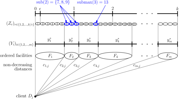
The ordering of the facilities is depicted in Figure 2, which also includes information about the fractional opening of facilities in $y^{*}$, i.e., facility $F_{i}$ is represented by an interval of length $y_{i}^{*}$. The total length of all intervals equals $k$. Next, we subdivide each interval into a set of (small) $\epsilon$-size pieces (called $\epsilon$-subintervals); $\epsilon$ is selected so that $\nicefrac{{1}}{{\epsilon}}$, and $\nicefrac{{y_{i}^{*}}}{{\epsilon}}$ for each $i$, are integers. Note that the values $y_{i}^{*}$, which originate from the solution returned by an LP solver, are rational numbers. The subdivision of $[0,k]$ into $\epsilon$-subintervals is shown in Figure 2 on the ”$(Z_{r})_{r\in\{1,2,\dots,\nicefrac{{k}}{{\epsilon}}\}}$” level.

The idea behind introducing the $\epsilon$-subintervals is the following. Although computationally the algorithm applies DR to the $y^{*}$ variables, for the sake of the analysis we may think that the DR process is actually rounding $z$ variables corresponding to $\epsilon$-subinterval under the additional assumption that rounding within individual facilities is done before rounding between facilities. Formally, we replace the vector $Y=(Y_{1},Y_{2},\dots,Y_{m})$ by an equivalent vector of random variables $Z=(Z_{1},Z_{2},\dots,Z_{\nicefrac{{k}}{{\epsilon}}})$. Random variable $Z_{r}$ represents the $r$-th $\epsilon$-subinterval. We will use the following notation to describe the bundles of $\epsilon$-subintervals that correspond to particular facilities:

$${{{\mathrm{submax}}}}(0)=0\qquad\text{and}\qquad{{{\mathrm{submax}}}}(i)={{{\mathrm{submax}}}}(i-1)+\frac{y_{i}^{*}}{\epsilon},$$ (6)

$${{{\mathrm{sub}}}}(i)=\{{{{\mathrm{submax}}}}(i-1)+1,\dots,{{{\mathrm{submax}}}}(i)\}.$$ (7)

Intuitively, ${{{\mathrm{sub}}}}(i)$ is the set of indexes $r$ such that $Z_{r}$ represents an interval belonging to the $i$-th facility. Examples for both definitions are shown in Figure 2 in the upper level. Formally, the random variables $Z_{r}$ are defined so that:

$$Y_{i}=\sum_{r\in{{{\mathrm{sub}}}}(i)}Z_{r}\qquad\text{and}\qquad Y_{i}=1\implies\exists!\;r\in{{{\mathrm{sub}}}}(i)\quad Z_{r}=1.$$ (8)

For each $r\in\{1,2,\dots,\nicefrac{{k}}{{\epsilon}}\}$ we can write that:

$$\mathrm{Pr}[Z_{r}=1]=\mathrm{Pr}[Z_{r}=1\big{|}Y_{{{{\mathrm{sub}}}}^{-1}(r)}=1]\cdot\mathrm{Pr}[Y_{{{{\mathrm{sub}}}}^{-1}(r)}=1]=\frac{\epsilon}{y_{{{{\mathrm{sub}}}}^{-1}(r)}^{*}}\cdot y_{{{{\mathrm{sub}}}}^{-1}(r)}^{*}=\epsilon$$ (9)

and $\mathrm{Pr}[Z_{r}=0]=1-\epsilon$, hence $\mathbb{E}[Z_{r}]=\epsilon$. Also we have:

$$\mathrm{Pr}\left[Y_{i}=1\right]=\mathrm{Pr}\left[\sum_{r\in{{{\mathrm{sub}}}}(i)}Z_{r}=1\right]=\mathrm{Pr}\left[\bigvee_{r\in{{{\mathrm{sub}}}}(i)}Z_{r}=1\right]=\sum_{r\in{{{\mathrm{sub}}}}(i)}\mathrm{Pr}\left[Z_{r}=1\right].$$ (10)

When $Y_{i}=1$ its representative is chosen randomly among $(Z_{r})_{r\in{{{\mathrm{sub}}}}(i)}$ independently of the choices of representatives of other facilities. Therefore

$$\forall_{i\in[m]}\quad\forall_{r\in{{{\mathrm{sub}}}}(i)}\quad\mathbb{E}\left[f(Y)\;|\;Y_{i}=1\right]=\mathbb{E}\left[f(Y)\;|\;Y_{i}=1\;\wedge\;Z_{r}=1\right],$$ (11)

for any function $f$ on vector $Y=(Y_{1},Y_{2},\dots,Y_{m})$.

Now we are ready to analyze the expected cost for any client $D_{j}\in\mathcal{D}$.

$$\mathbb{E}[{\mathrm{cost}}_{j}(Y)] \leq {\sum}_{i=1}^{m}\>\left(\mathbb{E}\left[{\frac{c_{ij}}{1+\sum_{i^{\prime}=1}^{i-1}Y_{i^{\prime}}}}\Bigg{|}Y_{i}=1\right]\cdot\mathrm{Pr}\left[Y_{i}=1\right]\right)$$ (12)

$$\stackrel{{\scriptstyle\eqref{eq:pr_sumZr}}}{{=}} {\sum}_{i=1}^{m}\>\left(c_{ij}\cdot\mathbb{E}\left[{\frac{1}{1+\sum_{i^{\prime}=1}^{i-1}Y_{i^{\prime}}}}\Bigg{|}Y_{i}=1\right]\cdot{\sum}_{r\in{{{\mathrm{sub}}}}(i)}\mathrm{Pr}\left[Z_{r}=1\right]\right)$$

$$= {\sum}_{i=1}^{m}\>\left(c_{ij}\cdot{\sum}_{r\in{{{\mathrm{sub}}}}(i)}\mathbb{E}\left[{\frac{1}{1+\sum_{i^{\prime}=1}^{i-1}Y_{i^{\prime}}}}\Bigg{|}Y_{i}=1\right]\cdot\mathrm{Pr}\left[Z_{r}=1\right]\right)$$

$$\stackrel{{\scriptstyle\eqref{eq:conditioning_Yi_Zr}}}{{=}} {\sum}_{i=1}^{m}\left(c_{ij}\cdot{\sum}_{r\in{{{\mathrm{sub}}}}(i)}\mathbb{E}\left[{\frac{1}{1+\sum_{i^{\prime}=1}^{i-1}Y_{i^{\prime}}}}\Bigg{|}Y_{i}=1\wedge Z_{r}=1\right]\cdot\mathrm{Pr}\left[Z_{r}=1\right]\right)$$

$$\stackrel{{\scriptstyle\eqref{eq:defZr},\eqref{eq:pr_zr1}}}{{=}} {\sum}_{i=1}^{m}\left(\epsilon\cdot c_{ij}\cdot{\sum}_{r\in{{{\mathrm{sub}}}}(i)}\mathbb{E}\left[{\frac{1}{1+\sum_{r^{\prime}=1}^{{{{\mathrm{submax}}}}(i-1)}Z_{r^{\prime}}}}\Bigg{|}Z_{r}=1\right]\right)$$

$$\stackrel{{\scriptstyle\eqref{eq:defZr}}}{{=}} {\sum}_{i=1}^{m}\left(\epsilon\cdot c_{ij}\cdot{\sum}_{r\in{{{\mathrm{sub}}}}(i)}\mathbb{E}\left[{\frac{1}{1+\sum_{r^{\prime}=1}^{r-1}Z_{r^{\prime}}}}\Bigg{|}Z_{r}=1\right]\right)$$

W.l.o.g., assume that ${\mathrm{OPT}}^{\mathrm{LP}}_{j}>0$. Hence the approximation ratio for any client $D_{j}$ is

$$\frac{\mathbb{E}[{\mathrm{cost}}_{j}(Y)]}{{\mathrm{OPT}}^{\mathrm{LP}}_{j}}\stackrel{{\scriptstyle\eqref{def:sub},\eqref{ineq:ecostjy}}}{{\leq}}\frac{{\sum}_{r=1}^{\nicefrac{{k}}{{\epsilon}}}\epsilon\cdot c_{{{{\mathrm{sub}}}}^{-1}(r),j}\cdot\mathbb{E}\left[{\frac{1}{1+\sum_{r^{\prime}=1}^{r-1}Z_{r^{\prime}}}}\bigg{|}Z_{r}=1\right]}{{\sum}_{r=1}^{\nicefrac{{k}}{{\epsilon}}}\epsilon\cdot c_{{{{\mathrm{sub}}}}^{-1}(r),j}\cdot\frac{1}{\lceil r\epsilon\rceil}}=$$

note that ${{{\mathrm{sub}}}}^{-1}(r)$ is an index of a facility that contains $Z_{r}$. Now we convert the sum over facilities into a sum over unit intervals. A unit interval is represented as a sum of $\nicefrac{{1}}{{\epsilon}}$ many $\epsilon$-subintervals:

$$= \frac{{\sum}_{\ell=1}^{k}\;{\sum}_{r=\nicefrac{{(\ell-1)}}{{\epsilon}}+1}^{\nicefrac{{\ell}}{{\epsilon}}}c_{{{{\mathrm{sub}}}}^{-1}(r),j}\cdot\mathbb{E}\left[{\frac{1}{1+\sum_{r^{\prime}=1}^{r-1}Z_{r^{\prime}}}}\bigg{|}Z_{r}=1\right]}{{\sum}_{\ell=1}^{k}\;{\sum}_{r=\nicefrac{{(\ell-1)}}{{\epsilon}}+1}^{\nicefrac{{\ell}}{{\epsilon}}}c_{{{{\mathrm{sub}}}}^{-1}(r),j}\cdot\frac{1}{\ell}}\leq$$

W.l.o.g., we can assume that first interval has non-zero costs: $\sum_{r=1}^{\nicefrac{{1}}{{\epsilon}}}c_{{{{\mathrm{sub}}}}^{-1}(r),j}>0$, otherwise the LP pays $0$ and our algorithm pays $0$ in expectation on intervals from non-empty prefix of $(1,2,\dots,k)$. With this assumption we can take maximum over intervals:

$$\stackrel{{\scriptstyle\text{Lemma \ref{lem:sai_over_sbi_leq_max_ai_over_bi}}}}{{\leq}} \max_{\ell\in[k]}\left(\frac{{\sum}_{r=\nicefrac{{(\ell-1)}}{{\epsilon}}+1}^{\nicefrac{{\ell}}{{\epsilon}}}c_{{{{\mathrm{sub}}}}^{-1}(r),j}\cdot\mathbb{E}\left[{\frac{1}{1+\sum_{r^{\prime}=1}^{r-1}Z_{r^{\prime}}}}\bigg{|}Z_{r}=1\right]}{{\sum}_{r=\nicefrac{{(\ell-1)}}{{\epsilon}}+1}^{\nicefrac{{\ell}}{{\epsilon}}}c_{{{{\mathrm{sub}}}}^{-1}(r),j}\cdot\frac{1}{\ell}}\right)\leq$$

Costs $c_{{{{\mathrm{sub}}}}^{-1}(r),j}$ can be general and they could be hard to analyze. Therefore we would like to remove costs from the analysis. We will use Lemma 18 for which the technique of splitting variables $Y_{i}$ into $Z_{r}$ was needed. We are using the fact that the variables $Z_{r}$ have the same expected values; otherwise the coefficient in front of the expected value would be $c_{ij}\cdot y_{i}^{*}$, i.e., not monotonic. Thus

$$\stackrel{{\scriptstyle\text{Lemma \ref{lem:ca_over_cb_leq_ab}}}}{{\leq}} \max_{\ell\in[k]}\;\left(\epsilon\cdot\ell\cdot{\sum}_{r=\nicefrac{{(\ell-1)}}{{\epsilon}}+1}^{\nicefrac{{\ell}}{{\epsilon}}}\;\mathbb{E}\left[{\frac{1}{1+\sum_{r^{\prime}=1}^{r-1}Z_{r^{\prime}}}}\bigg{|}Z_{r}=1\right]\right).$$ (13)

Consider the expected value in the above expression for a fixed $r\in\{\nicefrac{{(\ell-1)}}{{\epsilon}}+1,\dots,\nicefrac{{\ell}}{{\epsilon}}\}$:

$$E_{r} = \mathbb{E}\left[{\frac{1}{1+\sum_{r^{\prime}=1}^{r-1}Z_{r^{\prime}}}}\bigg{|}Z_{r}=1\right]={\sum}_{t=1}^{k}\frac{1}{t}\mathrm{Pr}\left[{\sum}_{r^{\prime}=1}^{r-1}Z_{r^{\prime}}=t-1\bigg{|}Z_{r}=1\right]=$$ (14)

$$= {\sum}_{t=1}^{\ell}\frac{1}{t}\mathrm{Pr}\left[{\sum}_{r^{\prime}=1}^{r-1}Z_{r^{\prime}}=t-1\bigg{|}Z_{r}=1\right]+{\sum}_{t=\ell+1}^{k}\frac{1}{t}\mathrm{Pr}\left[{\sum}_{r^{\prime}=1}^{r-1}Z_{r^{\prime}}=t-1\bigg{|}Z_{r}=1\right].$$

For $t\in\{1,2,\dots,\ell\}$ we consider the conditional probability in the above expression, denote it by $p_{r}(t-1)$, and analyze the corresponding cumulative distribution function $H_{r}(t-1)$:

$$p_{r}(t-1) = \mathrm{Pr}\left[{\sum}_{r^{\prime}=1}^{r-1}Z_{r^{\prime}}=t-1\bigg{|}Z_{r}=1\right],$$ (15)

$$H_{r}(t-1) = \mathrm{Pr}\left[{\sum}_{r^{\prime}=1}^{r-1}Z_{r^{\prime}}\leq t-1\bigg{|}Z_{r}=1\right]=\sum_{t^{\prime}=0}^{t-1}p_{r}(t^{\prime}),$$ (16)

We continue the analysis of $E_{r}$:

$$E_{r} \stackrel{{\scriptstyle\eqref{eq:Er},\eqref{eq:pz}}}{{=}} {\sum}_{t=1}^{\ell}\frac{1}{t}p_{r}(t-1)+{\sum}_{t=\ell+1}^{k}\frac{1}{t}p_{r}(t-1)$$ (17)

$$\stackrel{{\scriptstyle\eqref{eq:Hr_def}}}{{=}} H_{r}(0)+{\sum}_{t=2}^{\ell}\frac{1}{t}\left(H_{r}(t-1)-H_{r}(t-2)\right)+{\sum}_{t=\ell+1}^{k}\frac{1}{t}p_{r}(t-1)$$

$$= H_{r}(0)+{\sum}_{t=2}^{\ell}\frac{1}{t}H_{r}(t-1)-{\sum}_{t=2}^{\ell}\frac{1}{t}H_{r}(t-2)+{\sum}_{t=\ell+1}^{k}\frac{1}{t}p_{r}(t-1)$$

$$= {\sum}_{t=1}^{\ell}\frac{1}{t}H_{r}(t-1)-{\sum}_{t=1}^{\ell-1}\frac{1}{t+1}H_{r}(t-1)+{\sum}_{t=\ell+1}^{k}\frac{1}{t}p_{r}(t-1)$$

$$= {\sum}_{t=1}^{\ell-1}\frac{1}{t}H_{r}(t-1)-{\sum}_{t=1}^{\ell-1}\frac{1}{t+1}H_{r}(t-1)+\frac{1}{\ell}H_{r}(\ell-1)+{\sum}_{t=l+1}^{k}\frac{1}{t}p_{r}(t-1)$$

$$\leq {\sum}_{t=1}^{\ell-1}\left(\frac{1}{t}-\frac{1}{t+1}\right)H_{r}(t-1)+\frac{1}{\ell}\left(H_{r}(\ell-1)+{\sum}_{t=\ell+1}^{k}p_{r}(t-1)\right)$$

$$= {\sum}_{t=1}^{\ell-1}\frac{1}{t(t+1)}H_{r}(t-1)+\frac{1}{\ell}\left(H_{r}(\ell-1)+{\sum}_{t=\ell+1}^{k}p_{r}(t-1)\right)$$

$$\leq {\sum}_{t=1}^{\ell-1}\frac{1}{t(t+1)}H_{r}(t-1)+\frac{1}{\ell}.$$

Lemma 7.

For any $\ell\in[k]$, $t\in[\ell-1]$ and $r\in\{\nicefrac{{(\ell-1)}}{{\epsilon}}+1,\nicefrac{{(\ell-1)}}{{\epsilon}}+2,\dots,\nicefrac{{\ell}}{{\epsilon}}\}$ we have

$$H_{r}(t-1)\leq e^{-r\cdot\epsilon}\cdot\left(\frac{e\cdot r\cdot\epsilon}{t}\right)^{t}.$$

The proof of Lemma 7 combines the use of the BNA property of variables $\{Z_{1},Z_{2},\dots,Z_{\nicefrac{{k}}{{\epsilon}}}\}$ with applications of Chernoff-Hoeffding bounds. Due to the space constraints, the proof is moved to the Appendix C. In the end, we get the following bound on the approximation ratio.

Lemma 8.

For any $j\in[n]$ we have

$$\frac{\mathbb{E}[{\mathrm{cost}}_{j}(Y)]}{{\mathrm{OPT}}^{\mathrm{LP}}_{j}}\leq 2.3589.$$

A proof uses inequalities (13), (17) as well as Lemma 7 with an upper bound derived by an integral of the function $f_{t}(x)=e^{-x}$. We made numerical calculation for $\ell\in\{1,2,\dots,88\}$ and for other case we used Stirling formula and Taylor series for $e^{\ell}$ to derive analytical upper bound. Full proof, including a plot of numericaly obtained values, is presented in the Appendix C.

3 OWA $k$-median with Costs Satisfying the Triangle Inequality

In this section we construct an algorithm for OWA $k$-median with costs satisfying the triangle inequality. Thus, the problem we address in this section is more general than Harmonic $k$-median (i.e., the problem we have considered in the previous section) in a sense that we allow for arbitrary non-increasing sequences of weights. On the other hand, it is less general in a sense that we require the costs to form a specific structure (a metric).

In our approach we first adapt the algorithm of Hajiaghayi et al. [20] for Fault Tolerant $k$-median so that it applies to the following, slightly more general setting: for each client $D_{j}$ we introduce its multiplicity $m_{j}\in\mathbb{N}$—intuitively, this corresponds to cloning $D_{j}$ and co-locating all such clones in the same location as $D_{j}$. However, this will require a modification of the original algorithm for Fault Tolerant $k$-median, since we want to allow the multiplicities $\{m_{j}\}_{D_{j}\in\mathcal{D}}$ to be exponential with respect to the size of the instance (otherwise, we could simply copy each client a sufficient number of times, and use the original algorithm of Hajiaghayi et al.).

Next, we provide a reduction from OWA $k$-median to such a generalization of Fault Tolerant $k$-median. The resulting Fault Tolerant $k$-median with Clients Multiplicities problem can be cast as the following integer program:
$\displaystyle\text{min}\quad\sum_{j=1}^{n}$ $\displaystyle\sum_{i=1}^{m}\>m_{j}\cdot x_{ij}\cdot c_{ij}$ $\displaystyle\sum_{i=1}^{m}y_{i}=k$ $\displaystyle\sum_{i=1}^{m}x_{ij}$ $\displaystyle=r_{j}\qquad\;\>$ $\displaystyle\forall j\in[n]$ $\displaystyle x_{ij}$ $\displaystyle\leq y_{i}\qquad\;\>$ $\displaystyle\forall i\in[m],\;j\in[n]$ $\displaystyle y_{i},x_{ij}$ $\displaystyle\in\{0,1\}\quad$ $\displaystyle\forall i\in[m]$ $\displaystyle m_{j}$ $\displaystyle\in{{\mathbb{N}}}\qquad\;\>$ $\displaystyle\forall j\in[n]$

Theorem 9.

There is a polynomial-time $93$-approximation algorithm for Metric Fault Tolerant $k$-median with Clients Multiplicities.

Proof can be found in the Appendix D.

Consider reduction from OWA $k$-median to Fault Tolerant $k$-median with Clients Multiplicities depicted on Figure 3.

Reduction.

Let us take an instance $I$ of OWA $k$-median $\big{(}\mathcal{D},\mathcal{F},k,w,\{c_{ij}\}_{F_{i}\in\mathcal{F},D_{j}\in\mathcal{D}}\big{)}$ where $w_{i}=\frac{p_{i}}{q_{i}},i\in[k]$ are rational numbers in the canonical form. We construct an instance $I^{\prime}$ of Fault Tolerant $k$-median with Clients Multiplicities with the same set of facilities and the same number of facilities to open, $k$. Each client $D_{j}\in\mathcal{D}$ is replaced with clients $D_{j,1},D_{j,2},\dots,D_{j,k}$ with requirements $1,2,\dots,k$, respectively. For $Q=\prod_{r=1}^{k}q_{r}$, the multiples of the clients are defined as follows:

• $m_{j,\ell}=(w_{\ell}-w_{\ell+1})\cdot Q$, for each $\ell\in[k-1]$, and

• $m_{j,k}=w_{k}\cdot Q$.

Figure 3: Reduction from OWA $k$-median to Fault Tolerant $k$-median with Clients Multiplicities.

Lemma 10.

Let $I$ be an instance of OWA $k$-median, and let $I^{\prime}$ be an instance of Fault Tolerant $k$-median with Clients Multiplicities constructed from $I$ through reduction from Figure 3. An $\alpha$-approximate solution to $I^{\prime}$ is also an $\alpha$-approximate solution to $I$.

Proof can be found in the Appendix D.

Corollary 11.

There exists a $93$-approximation algorithm for Metric OWA $k$-median that runs in polynomial time.

4 Concluding Remarks and Open Questions

We have introduced a new family of $k$-median problems, called OWA $k$-median, and we have shown that our problem with the harmonic sequence of weights allows for a constant factor approximation even for general (non-metric) costs. This algorithm applies to Proportional Approval Voting. In the analysis of our approximation algorithm for Harmonic $k$-median, we used the fact that the dependent rounding procedure satisfies Binary Negative Association.

We showed that any Metric OWA $k$-median can be approximated within a factor of $93$ via a reduction to Fault Tolerant $k$-median with Clients Multiplicities. We also obtained that OWA $k$-median with $p$-geometric weights with $p<\nicefrac{{1}}{{e}}$ cannot be approximated without the assumption of the costs being metric. The status of the non-metric problem with $p$-geometric weights with $p>\nicefrac{{1}}{{e}}$ remains an intriguing open problem.

Using approximation and randomized algorithms for finding winners of elections requires some comment. First, the multiwinner election rules such as PAV have many applications in the voting theory, recommendation systems and in resource allocation. Using (randomized) approximation algorithms in such scenarios is clearly justified. However, even for other high-stake domains, such as political elections, the use of approximation algorithms is a promising direction. One approach is to view an approximation algorithm as a new, full-fledged voting rule (for more discussion on this, see the works of Caragiannis et al. [7, 8], Skowron et al. [33], and Elkind et al. [15]). In fact, the use of randomized algorithms in this context has been advocated in the literature as well—e.g., one can arrange an election where each participant is allowed to suggest a winning committee, and the best out of the suggested committees is selected; in such case the approximation guaranty of the algorithm corresponds to the quality of the outcome of elections (for a more detailed discussion see [33]) . Nonetheless, we think that it would be beneficial to learn whether our algorithm can be efficiently derandomized.

Appendix A Dependent Rounding and Negative Association

Consider a vector of $m$ variables $(y_{i})_{i\in[m]}$, and let $y^{*}_{i}$ denote the initial value of the variable $y_{i}$. For simplicity we will assume that $0\leq y^{*}_{i}\leq 1$ for each $i$, and that $k=\sum_{i\in[m]}y^{*}_{i}$ is an integer. A rounding procedure takes this vector of (fractional) variables as an input, and transforms it into a vector of 0/1 integers. We focus on a specific rounding procedure studied by Srinivasan [34] which we refer to as dependent rounding (DR).

DR works in steps: in each step it selects two fractional variables, say $y_{i}$ and $y_{j}$, and changes the values of these variables to $y_{i}^{\prime}$ and $y_{j}^{\prime}$ so that $y_{i}^{\prime}+y_{j}^{\prime}=y_{i}+y_{j}$, and so that $y_{i}^{\prime}$ or $y_{j}^{\prime}$ is an integer. Thus, after each iteration at least one additional variable becomes an integer. The rounding procedure stops, when all variables are integers. In each step the randomization is involved: with some probability $p$ variable $y_{i}$ is rounded to an integer value, and with probability $1-p$ variable $y_{j}$ becomes an integer. The value of the probability $p$ is selected so as to preserve the expected value of each individual entry $y_{i}$. Clearly, if $y_{i}+y_{j}\geq 1$, then one of the variables is rounded to 1; otherwise, one of the variables is rounded to 0. For example, if $y_{i}=0.4$ and $y_{j}=0.8$, then with probability $0.25$ the values of the variables $y_{i}$ and $y_{j}$ change to, respectively, $1$ and $0.2$; and with probability $0.75$ they change to, respectively, $0.2$ and $1$. If $y_{i}=0.3$ and $y_{j}=0.2$, then with probability $0.4$ the values of the two variables change to, respectively, $0$ and $0.5$; and with probability $0.6$, to, respectively, $0.5$ and $0$.

Let $Y_{i}$ denote the random variable which returns one if $y_{i}$ is rounded to one after the whole rounding procedure, and zero, otherwise. It was shown [34] that the DR generates distributions of $Y_{i}$ which satisfy the following three properties:

Marginals.

$\mathrm{Pr}[Y_{i}=1]=y^{*}_{i}$,

Sum Preservation.

$\mathrm{Pr}[\sum_{i}Y_{i}=k]=1$,

Negative Correlation.

For each $S\subseteq[m]$ it holds that $\mathrm{Pr}[\bigwedge_{i\in S}(Y_{i}=1)]\leq\prod_{i\in S}\mathrm{Pr}[Y_{i}=1]$, and $\mathrm{Pr}[\bigwedge_{i\in S}(Y_{i}=0)]\leq\prod_{i\in S}\mathrm{Pr}[Y_{i}=0]$.

These three properties are often used in the analysis of approximation algorithms based on dependent rounding for various optimization problems—see, e.g., [18]. In fact, DR satisfies an even stronger property than NC, called conditional negative association (CNA) [27], yet, to the best of our knowledge, this property has never been used before for analyzing algorithms based on the DR procedure.

For two random variables, $X$ and $Y$, by $\mathrm{cov}[X,Y]$ we denote the covariance between $X$ and $Y$. Recall that $\mathrm{cov}[X,Y]=\mathbb{E}[XY]-\mathbb{E}[X]\cdot\mathbb{E}[Y]$.

Negative Association [23].

For each $S,Q\subseteq[m]$ with $S\cap Q=\emptyset$, $s=|S|$, and $q=|Q|$, and each two nondecreasing functions, $f\colon[0,1]^{s}\to{{\mathbb{R}}}$ and $g\colon[0,1]^{q}\to{{\mathbb{R}}}$, it holds that:

$$\mathrm{cov}\big{[}f(Y_{i}\colon i\in S),g(Y_{i}\colon i\in Q)\big{]}\leq 0.$$

Conditional Negative Association.

We say that the sequence of random variables $(Y_{i})_{i\in[m]}$ satisfies the CNA property if the conditional variables $(Y_{[m]\setminus S}|Y_{S}=a)$ satisfy NA for any $S\subseteq[m]$ and any $a=(a_{i})_{i\in S}$. For $S=\emptyset$, CNA is equivalent to NA. It was shown by Dubhashi et al. [13] that if one rounds the variables according to a predefined linear order over the variables $\succ$ (i.e., if one always chooses for rounding the two fractional variables which are earliest in $\succ$), then the resulting distribution satisfies CNA. Yet, the requirement of following a predefined linear order of variables is too restrictive for our needs. Then, Kramer et al. [27] showed that DR following a predefined order on pairs of variables that implements a tournament tree returns a distribution satisfying CNA.

In our analysis we will use a simpler version of the NA property, which nevertheless is expressive enough for our needs. We introduce the following property.

Binary Negative Association (BNA).

For each $S,Q\subseteq[m]$ with $S\cap Q=\emptyset$, $s=|S|$, and $q=|Q|$, and each two nondecreasing functions, $f\colon\{0,1\}^{s}\to\{0,1\}$ and $g\colon\{0,1\}^{q}\to\{0,1\}$, we have:

$$\mathrm{cov}\big{[}f(Y_{i}\colon i\in S),g(Y_{i}\colon i\in Q)\big{]}\leq 0.$$

From the definitions it is easy to see that CNA $\implies$ NA $\implies$ BNA.

A.1 BNA is Strictly Stronger than NC

We now argue that BNA is a strictly stronger property than NC. First we show a straightforward inductive argument that BNA implies NC. Next we provide an example of a distribution that satisfies NC but not BNA. In fact, this distribution is generated by a not-careful-enough implementation of DR.

Lemma 12.

For two binary random variables $X$, and $Y$, $X,Y\in\{0,1\}$, the condition $\mathrm{cov}[X,Y]\leq 0$ is equivalent to $\mathrm{Pr}[X=1\wedge Y=1]\leq\mathrm{Pr}[X=1]\cdot\mathrm{Pr}[Y=1]$.

Proof.

Observe that for binary variables, $X$ and $Y$, it holds that $\mathbb{E}[X]=\mathrm{Pr}[X=1]$, $\mathbb{E}[Y]=\mathrm{Pr}[Y=1]$, and $\mathbb{E}[XY]=\mathrm{Pr}[X=1\wedge Y=1]$. ∎

Lemma 13.

Binary Negative Association of $(Y_{i})_{i\in[m]}$ implies their Negative Correlation.

Proof.

We will prove the NC property by induction on $|S|$. Clearly, the property holds for $|S|=1$. For an inductive step, we define two non-decreasing functions $f(Y_{i}\colon i\in S/\{j\})=\bigwedge_{i\in S/\{j\}}(Y_{i}=1)$ and $g(Y_{j})=(Y_{j}=1)$ for any $j\in S$.

$$\mathrm{Pr}\left[\bigwedge_{i\in S}(Y_{i}=1)\right] = \mathrm{Pr}\left[\bigwedge_{i\in S/\{j\}}(Y_{i}=1)\;\wedge\;Y_{j}=1\right]$$

$$\stackrel{{\scriptstyle\text{BNA, Lemma~{}\ref{lem:cov_for_binary}}}}{{\leq}} \mathrm{Pr}\left[\bigwedge_{i\in S/\{j\}}(Y_{i}=1)\right]\cdot\mathrm{Pr}\left[Y_{j}=1\right]$$

$$\stackrel{{\scriptstyle\text{inductive assum.}}}{{\leq}} \prod_{i\in S}\mathrm{Pr}[Y_{i}=1].$$

In order to bound the probability of $\bigwedge_{i\in S}(Y_{i}=0)$ we define two other non-decreasing functions $f(Y_{i}\colon i\in S/\{j\})=\bigvee_{i\in S/\{j\}}(Y_{i}>0)$ and $g(Y_{j})=(Y_{j}>0)$ for any $j\in S$.

$$\mathrm{Pr}\left[\bigwedge_{i\in S}(Y_{i}=0)\right] =\hskip 5.69046pt1-\mathrm{Pr}\left[\bigvee_{i\in S}(Y_{i}>0)\right]$$

$$= 1-\left(\mathrm{Pr}\left[\bigvee_{i\in S/\{j\}}(Y_{i}>0)\right]+\mathrm{Pr}\left[Y_{j}>0\right]-\mathrm{Pr}\left[\bigvee_{i\in S/\{j\}}(Y_{i}>0)\;\wedge\;Y_{j}>0\right]\right)$$

$$= \mathrm{Pr}\left[\bigwedge_{i\in S/\{j\}}(Y_{i}=0)\right]-\mathrm{Pr}\left[Y_{j}>0\right]+\mathrm{Pr}\left[\bigvee_{i\in S/\{j\}}(Y_{i}>0)\;\wedge\;Y_{j}>0\right]$$

$$\stackrel{{\scriptstyle\text{BNA, Lemma~{}\ref{lem:cov_for_binary}}}}{{\leq}} \mathrm{Pr}\left[\bigwedge_{i\in S/\{j\}}(Y_{i}=0)\right]-\mathrm{Pr}\left[Y_{j}>0\right]+\mathrm{Pr}\left[\bigvee_{i\in S/\{j\}}(Y_{i}>0)\right]\cdot\mathrm{Pr}\left[Y_{j}>0\right]$$

$$= \mathrm{Pr}\left[\bigwedge_{i\in S/\{j\}}(Y_{i}=0)\right]-\mathrm{Pr}\left[Y_{j}>0\right]\cdot\mathrm{Pr}\left[\bigwedge_{i\in S/\{j\}}(Y_{i}=0)\right]$$

$$= \mathrm{Pr}\left[\bigwedge_{i\in S/\{j\}}(Y_{i}=0)\right]\cdot\mathrm{Pr}\left[Y_{j}=0\right]\stackrel{{\scriptstyle\text{inductive assum.}}}{{\leq}}\prod_{i\in S}\mathrm{Pr}[Y_{i}=0].$$

∎

Note that the general formulation of DR does not specify how the pairs of fractional variables are selected. The proof in [34] that DR satisfies NC is independent of the method in which these pairs of fractional variables are selected. We will now show that, if these pairs are selected by an adaptive adversary who may take into account the way in which the previous pairs were rounded, then the BNA property may not hold (so, also neither NA nor CNA). Consider the following example.

Example 14.

Consider $m=8,k=4$, and the vector of variables $(y_{i})_{i\in[8]}$, all with the same initial value $\nicefrac{{1}}{{2}}$. Let $S=\{2,3,4\}$, $Q=\{5\}$, and:

$$f(Y_{2},Y_{3},Y_{4})=\begin{cases}1&\quad\text{if~{}~{}}Y_{2}+Y_{3}+Y_{4}\geq 2\\ 0&\quad\text{otherwise}\\ \end{cases}\quad\quad g(Y_{5})=Y_{5}\text{.}$$

Let $\alpha$ and $\beta$ denote the events that $Y_{2}+Y_{3}+Y_{4}\geq 2$ and that $Y_{5}=1$, respectively. BNA would require that $\mathrm{Pr}[\alpha\wedge\beta]\leq\mathrm{Pr}[\alpha]\cdot\mathrm{Pr}[\beta]$. Consider DR procedure as depicted in the following diagram (the paired variables are enclosed in rounded rectangles). First, we pair variables $y_{1}$ with $y_{5}$ and $y_{2}$ with $y_{6}$. The way in which the remaining variables are paired depends on the result of rounding within pairs $(y_{1},y_{5})$ and $(y_{2},y_{6})$. If $y_{1}$ and $y_{2}$ are both rounded to the same integer, then we pair $y_{3}$ with $y_{7}$ and $y_{4}$ with $y_{8}$. Otherwise, we pair $y_{3}$ with $y_{4}$ and $y_{7}$ with $y_{8}$.

Figure 4: An illustration of Example 14.

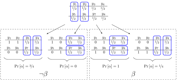
Note that according to DR each rounding decision is taken with the same probability (e.g., when we pair variables $y_{1}$ with $y_{5}$, then the probabilities of $y_{1}$ and $y_{5}$ rounded to one is the same). Thus, we observe that $\mathrm{Pr}[\alpha]=\nicefrac{{1}}{{2}}$, $\mathrm{Pr}[\beta]=\nicefrac{{1}}{{2}}$, but $\mathrm{Pr}[\alpha\wedge\beta]=\nicefrac{{1}}{{4}}+\nicefrac{{1}}{{16}}$.

Example 14 is simpler than the one given by Kramer et al. [27]. Both examples show that NA is a strictly stronger property than NC. Kramer et al. use the set of 7 variables with initial values equal to $\nicefrac{{3}}{{7}}$, $k=4$, and a predefined order on pairs of variables. Our example uses an adaptive adversary who decides which pair of variables should be rounded in each step of the rounding procedure. Our example cannot be implemented by fixing an order on pairs of variables (hence it also cannot be implemented by fixing a tournament tree). Our 8 variables have marginal probabilities equal to $\nicefrac{{1}}{{2}}$, thus the example can be easily understood, and one does not need to calculate probabilities of choosing all ${7\choose 4}$ 4-element sets.

A.2 Fixed Tournament Pairings Ensure BNA

The method in which fractional elements are paired together can be thought of as a subset of rules of a sports tournament, in which losers drop out of the game, but winners remain and are being paired up for the following games. The above example shows that an awkward adaptive pairing of remaining players may influence the value of certain functions on the subsets of players. We will show that if the competition is organized by a standard fixed upfront tournament tree, then such manipulations are not possible, which allows to prove BNA for the outcome of the DR process following such tree.

Intuitively, the way in which the variables are paired should be, in some sense, independent of the result of previous roundings. We consider a fixed binary tree with $m$ leaves—each leaf containing one variable $y_{i}$ with value $y^{*}_{i}$, so that each variable is put in exactly one leaf; the other nodes are temporarily empty. In each step, the algorithm selects two nonempty nodes, say $n_{1}$ and $n_{2}$, with a common empty parent, and applies the basic step of the DR procedure to the two variables in nodes $n_{1}$ and $n_{2}$. As a result at least one of the variables becomes an integer. If one of the variables is still fractional, we promote this variable with its new value to the parent node. If both variables become integers (which happens when their sum is equal to one), we promote a fake variable $\bot$ to the parent node. When we compare any variable $v$ with $\bot$, we always promote $v$ with its current value to the parent node. An example run of such implementation of the DR procedure is depicted in Figure 5.

Figure 5: An example run of DR using a tournament tree structure. In this example the result is: $y_{2},y_{3},y_{6}=1$, and $y_{1},y_{4},y_{5}=0$.

Hereinafter we assume that the DR procedure uses a fixed tournament tree structure, as described above.

Theorem 15.

The DR algorithm using a tournament tree structure guarantees BNA.

The proof follows from Theorem 5 in [27]. The theorem says that DR using a tournament tree structure produces distributions satisfying the NA property; clearly, NA implies BNA. However, to make the paper self-contained, we provide our inductive proof of Theorem 15 in the remainder of the section. Our proof uses induction on the number of fractional variables; Kramer et al. [27] use induction on the number of leaves in the tournament tree. While the two proofs use similar ideas and are of a similar difficulty, our proof is slightly more direct and shorter.

Proof of Theorem 15.

Recall that $Y_{i}$ is a random variable that indicates whether or not the described DR procedure rounds $y_{i}$ to 1. Let $S,Q\subseteq[m]$ with $S\cap Q=\emptyset$, $s=|S|$, and $q=|Q|$, and let $f\colon\{0,1\}^{s}\to\{0,1\}$ and $g\colon\{0,1\}^{q}\to\{0,1\}$ be two nondecreasing functions. Let $\alpha$ and $\beta$ denote the events that $f(Y_{i}\colon i\in S)=1$ and $g(Y_{i}\colon i\in Q)=1$, respectively.

For a vector $\overline{y}$ of $m$ values, which represents the values of the variables $(y_{i})_{i\in[m]}$ that appear during our rounding procedure by $\mathrm{Pr}\left[E|\overline{y}\right]$ we denote the probability that an event $E$ occurs under the condition that we have reached the point of the rounding algorithm where the variables $(y_{i})_{i\in[m]}$ have values indicated by $\overline{y}$. By Lemma 12 it is sufficient to show that the following inequality holds for each $\overline{y}$:

$$\mathrm{Pr}\left[\alpha\wedge\beta|\overline{y}\right]\leq\mathrm{Pr}\left[\alpha|\overline{y}\right]\cdot\mathrm{Pr}\left[\beta|\overline{y}\right].$$ (18)

We will prove this statement by induction on the number of fractional variables in $\overline{y}$. If $\overline{y}$ contains only integer variables, then it is clear that Inequality (18) is satisfied. Now assume that Inequality (18) is satisfied whenever $\overline{y}$ contains at most $\ell$ fractional values. We will show that Inequality (18) is also satisfied when $\overline{y}$ contains $\ell+1$ fractional values. Let $\overline{y}$ be such vector. Consider a single step of our algorithm, where the two variables $y_{i}$ and $y_{j}$ are paired. Let $E_{i}$ and $E_{j}$ denote the events that, respectively, $y_{i}$ and $y_{j}$, is increased. Similarly, let $\overline{y(i)}$ and $\overline{y(j)}$ denote the vectors of the values of the variables $(y_{i})_{i\in[m]}$ when, respectively, $y_{i}$ and $y_{j}$ is increased. We have:

$$\mathrm{Pr}\left[\alpha\wedge\beta|\overline{y}\right]=\mathrm{Pr}\left[\alpha\wedge\beta|\overline{y(i)}\right]\cdot\mathrm{Pr}\left[E_{i}\right]+\mathrm{Pr}\left[\alpha\wedge\beta|\overline{y(j)}\right]\cdot\mathrm{Pr}\left[E_{j}\right]\text{.}$$

By our inductive assumption, it holds that:

$$\mathrm{Pr}\left[\alpha\wedge\beta|\overline{y}\right]\leq\mathrm{Pr}\left[\alpha|\overline{y(i)}\right]\cdot\mathrm{Pr}\left[\beta|\overline{y(i)}\right]\cdot\mathrm{Pr}\left[E_{i}\right]+\mathrm{Pr}\left[\alpha|\overline{y(j)}\right]\cdot\mathrm{Pr}\left[\beta|\overline{y(j)}\right]\cdot\mathrm{Pr}\left[E_{j}\right]\text{.}$$ (19)

Now, we consider the following cases:

Case 1: $i,j\notin S$.

Observe that either the fake variable $\bot$ is promoted to the parent node or one of the variables: $y_{i}$ and $y_{j}$. Observe that irrespectively of which of the two variables is promoted to the parent, the promoted variable will always hold the same new value. Further, observe that the subsequent rounding steps do not depend on which variable has been promoted to the parent node, but only on the value of the promoted variable. Thus, the rounding within the pair of variables, $y_{i}$ and $y_{j}$, affects only the probability of events including $Y_{i}$ or $Y_{j}$ (here we use the assumption that the tournament tree is fixed; the way in which the variables are paired does not depend on the result of rounding within the pair $(y_{i},y_{j})$). In particular, $\mathrm{Pr}\left[\alpha|\overline{y(i)}\right]=\mathrm{Pr}\left[\alpha|\overline{y}\right]$ and $\mathrm{Pr}\left[\alpha|\overline{y(j)}\right]=\mathrm{Pr}\left[\alpha|\overline{y}\right]$. We can rewrite Inequality (19) as follows:

$$\mathrm{Pr}\left[\alpha\wedge\beta|\overline{y}\right] \leq\mathrm{Pr}\left[\alpha|\overline{y}\right]\cdot\mathrm{Pr}\left[\beta|\overline{y(i)}\right]\cdot\mathrm{Pr}\left[E_{i}\right]+\mathrm{Pr}\left[\alpha|\overline{y}\right]\cdot\mathrm{Pr}\left[\beta|\overline{y(j)}\right]\cdot\mathrm{Pr}\left[E_{j}\right]$$

$$=\mathrm{Pr}\left[\alpha|\overline{y}\right]\Big{(}\mathrm{Pr}\left[\beta|\overline{y(i)}\right]\cdot\mathrm{Pr}\left[E_{i}\right]+\mathrm{Pr}\left[\beta|\overline{y(j)}\right]\cdot\mathrm{Pr}\left[E_{j}\right]\Big{)}$$

$$=\mathrm{Pr}\left[\alpha|\overline{y}\right]\cdot\mathrm{Pr}\left[\beta|\overline{y}\right]\text{.}$$

Case 2: $i,j\notin Q$.

The same reasoning but applied to $\beta$ rather than to $\alpha$, leads to the same conclusion.

Case 3: $i\in S$ and $j\in Q$ (the case when $i\in Q$ and $j\in S$ is symmetric).

As a result of rounding, one of the variables, $y_{i}$ and $y_{j}$, increases, and the other one decreases. Let us analyze what happens when $y_{i}$ increases and $y_{j}$ decreases, i.e., when event $E_{i}$ occurs. By the same reasoning as in Case 1, we infer that the fact that $y_{i}$ is increased does not influence the further process of rounding other variables than $y_{i}$ and $y_{j}$. At the same time when $y_{i}$ is increased, it becomes more likely that this variable will eventually become one, in comparison to the case when $y_{j}$ is increased:

1. If $y_{i}+y_{j}\geq 1$, then $y_{i}$ being increased means that $y_{i}$ becomes one right away.

2. Otherwise, i.e., if $y_{i}+y_{j}<1$: if $y_{i}$ is increased, it is still positive so it is still possible that it will eventually become one. On the other hand, if $y_{j}$ is increased, then $y_{i}$ is rounded down to zero, which makes it impossible for $y_{i}$ to become one.

Since the function $f$ is nondecreasing we infer that $\mathrm{Pr}\left[\alpha|\overline{y(i)}\right]\geq\mathrm{Pr}\left[\alpha|\overline{y(j)}\right]$. The same reasoning allows us to conclude that $\mathrm{Pr}\left[\beta|\overline{y(i)}\right]\leq\mathrm{Pr}\left[\beta|\overline{y(j)}\right]$. This is summarized in the following claim:

Claim 1.

$\mathrm{Pr}\left[\alpha|\overline{y(i)}\right]\geq\mathrm{Pr}\left[\alpha|\overline{y(j)}\right]$ and $\mathrm{Pr}\left[\beta|\overline{y(i)}\right]\leq\mathrm{Pr}\left[\beta|\overline{y(j)}\right]$.

At the same time:

$$\begin{split}\mathrm{Pr}\left[\beta|\overline{y(i)}\right]\cdot\mathrm{Pr}\left[E_{i}\right]+\mathrm{Pr}\left[\beta|\overline{y(j)}\right]\cdot\mathrm{Pr}\left[E_{j}\right]&=\mathrm{Pr}\left[\beta|\overline{y}\right]\\ &=\mathrm{Pr}\left[\beta|\overline{y}\right]\big{(}\mathrm{Pr}\left[E_{i}\right]+\mathrm{Pr}\left[E_{j}\right]\big{)}.\end{split}$$ (20)

Claim 2.

It holds that:

1. $\mathrm{Pr}\left[\beta|\overline{y(i)}\right]\mathrm{Pr}\left[E_{i}\right]\leq\mathrm{Pr}\left[\beta|\overline{y}\right]\mathrm{Pr}\left[E_{i}\right]$, and

2. $\mathrm{Pr}\left[\beta|\overline{y(j)}\right]\mathrm{Pr}\left[E_{j}\right]\geq\mathrm{Pr}\left[\beta|\overline{y}\right]\mathrm{Pr}\left[E_{j}\right]$.

Proof of Claim 2.

For the sake of contradiction, let us assume that one of these inequalities is not satisfied, say assume that $\mathrm{Pr}\left[\beta|\overline{y(i)}\right]\mathrm{Pr}\left[E_{i}\right]>\mathrm{Pr}\left[\beta|\overline{y}\right]\mathrm{Pr}\left[E_{i}\right]$. By Equality (20) we get that also $\mathrm{Pr}\left[\beta|\overline{y(j)}\right]\mathrm{Pr}\left[E_{j}\right]<\mathrm{Pr}\left[\beta|\overline{y}\right]\mathrm{Pr}\left[E_{j}\right]$. In these two conditions we can reduce the factors $\mathrm{Pr}\left[E_{i}\right]$ and $\mathrm{Pr}\left[E_{j}\right]$, respectively, and obtain that $\mathrm{Pr}\left[\beta|\overline{y(i)}\right]>\mathrm{Pr}\left[\beta|\overline{y}\right]$ and $\mathrm{Pr}\left[\beta|\overline{y(j)}\right]<\mathrm{Pr}\left[\beta|\overline{y}\right]$. By combining these two inequalities, we get that $\mathrm{Pr}\left[\beta|\overline{y(i)}\right]>\mathrm{Pr}\left[\beta|\overline{y(j)}\right]$, which contradicts Claim 1. ∎

Now, we continue the proof of Theorem 15. We will apply Lemma 19 with:

1. $a_{1}=\mathrm{Pr}\left[\alpha|\overline{y(i)}\right]$, $a_{2}=\mathrm{Pr}\left[\alpha|\overline{y(j)}\right]$,

2. $b_{1}=\mathrm{Pr}\left[\beta|\overline{y(i)}\right]\mathrm{Pr}\left[E_{i}\right]$, $b_{2}=\mathrm{Pr}\left[\beta|\overline{y(j)}\right]\mathrm{Pr}\left[E_{j}\right]$,

3. $c_{1}=\mathrm{Pr}\left[\beta|\overline{y}\right]\mathrm{Pr}\left[E_{i}\right]$, and $c_{2}=\mathrm{Pr}\left[\beta|\overline{y}\right]\mathrm{Pr}\left[E_{j}\right]$.

($a_{1}\geq a_{2}$ by Claim 1; $c_{1}\geq b_{1}$ and $b_{2}\geq c_{2}$, by Claim 2; $b_{1}+b_{2}=c_{1}+c_{2}$ by Equality (20)). We get that:

$$\mathrm{Pr}\left[\alpha|\overline{y(i)}\right]\cdot\mathrm{Pr}\left[\beta|\overline{y(i)}\right]\cdot\mathrm{Pr}\left[E_{i}\right]+\mathrm{Pr}\left[\alpha|\overline{y(j)}\right]\cdot\mathrm{Pr}\left[\beta|\overline{y(j)}\right]\cdot\mathrm{Pr}\left[E_{j}\right]\leq$$

$$\mathrm{Pr}\left[\alpha|\overline{y(i)}\right]\cdot\mathrm{Pr}\left[\beta|\overline{y}\right]\cdot\mathrm{Pr}\left[E_{i}\right]+\mathrm{Pr}\left[\alpha|\overline{y(j)}\right]\cdot\mathrm{Pr}\left[\beta|\overline{y}\right]\cdot\mathrm{Pr}\left[E_{j}\right].$$

Combining the above inequality with Inequality (19), we infer that:

$$\mathrm{Pr}\left[\alpha\wedge\beta|\overline{y}\right] \leq\mathrm{Pr}\left[\alpha|\overline{y(i)}\right]\cdot\mathrm{Pr}\left[\beta|\overline{y}\right]\cdot\mathrm{Pr}\left[E_{i}\right]+\mathrm{Pr}\left[\alpha|\overline{y(j)}\right]\cdot\mathrm{Pr}\left[\beta|\overline{y}\right]\cdot\mathrm{Pr}\left[E_{j}\right]$$

$$=\mathrm{Pr}\left[\beta|\overline{y}\right]\Big{(}\mathrm{Pr}\left[\alpha|\overline{y(i)}\right]\cdot\mathrm{Pr}\left[E_{i}\right]+\mathrm{Pr}\left[\alpha|\overline{y(j)}\right]\cdot\mathrm{Pr}\left[E_{j}\right]\Big{)}$$

$$=\mathrm{Pr}\left[\beta|\overline{y}\right]\cdot\mathrm{Pr}\left[\alpha|\overline{y}\right]$$

This proves the inductive step and completes the proof. ∎

Appendix B Useful Lemmas

Theorem 16 (Theorem 1.16 from [3]).

Let $X_{1},X_{2},\dots,X_{n}$ be negatively correlated binary random variables. Let $X=\sum_{i=1}^{n}X_{i}$. Then $X$ satisfies the Chernoff-Hoeffding bounds for $\delta\in[0,1]$:

$$\mathrm{Pr}\left[X\leq(1-\delta)\mathbb{E}[X]\right]\leq\left(\frac{e^{-\delta}}{(1-\delta)^{(1-\delta)}}\right)^{\mu}.$$

Lemma 17.

For any sequence $(a_{i})_{i\in[n]}$ and $(b_{i})_{i\in[n]}$, $b_{i}>0$, it holds:

$$\frac{\sum_{i=1}^{n}a_{i}}{\sum_{i=1}^{n}b_{i}}\leq\max_{i\in\{1,2,\dots,n\}}\frac{a_{i}}{b_{i}}.$$

Proof.

$$\frac{\sum_{i=1}^{n}a_{i}}{\sum_{i=1}^{n}b_{i}} = \sum_{j=1}^{n}\frac{a_{j}}{\sum_{i=1}^{n}b_{i}}=\sum_{j=1}^{n}\frac{a_{j}}{b_{j}}\cdot\frac{b_{j}}{\sum_{i=1}^{n}b_{i}}\leq\sum_{j=1}^{n}\left(\max_{i\in\{1,2,\dots,n\}}\frac{a_{i}}{b_{i}}\right)\frac{b_{j}}{\sum_{i=1}^{n}b_{i}}=$$

$$= \left(\max_{i\in\{1,2,\dots,n\}}\frac{a_{i}}{b_{i}}\right)\sum_{j=1}^{n}\frac{b_{j}}{\sum_{i=1}^{n}b_{i}}=\max_{i\in\{1,2,\dots,n\}}\frac{a_{i}}{b_{i}}.$$

∎

Lemma 18.

For any non-decreasing sequence $(c_{i})_{i\in\{1,2,\dots,n\}}$, $c_{i}>0$ and any non-increasing sequence $(a_{i})_{i\in\{1,2,\dots,n\}}$ it holds:

$$\frac{\sum_{i=1}^{n}a_{i}c_{i}}{\sum_{i=1}^{n}c_{i}}\leq\frac{1}{n}\sum_{i=1}^{n}a_{i}.$$

Proof.

We prove that by induction. Clearly, we have equality for $n=1$. We assume that

$$\frac{\sum_{i=1}^{n-1}a_{i}c_{i}}{\sum_{i=1}^{n-1}c_{i}}\leq\frac{1}{n-1}\sum_{i=1}^{n-1}a_{i}.$$

It is equivalent to

$$(n-1)\cdot\sum_{i=1}^{n-1}a_{i}c_{i}\leq\left(\sum_{i=1}^{n-1}a_{i}\right)\cdot\left(\sum_{i=1}^{n-1}c_{i}\right).$$ (21)

We would like to show that

$$n\cdot\sum_{i=1}^{n}a_{i}c_{i}\leq\left(\sum_{i=1}^{n}a_{i}\right)\cdot\left(\sum_{i=1}^{n}c_{i}\right).$$

We have the following equivalent inequalities:

$$0 \leq \left(\sum_{i=1}^{n-1}a_{i}\right)\cdot\left(\sum_{i=1}^{n-1}c_{i}\right)+a_{n}\cdot\sum_{i=1}^{n-1}c_{i}+c_{n}\cdot\sum_{i=1}^{n-1}a_{i}+a_{n}\cdot c_{n}-n\cdot\sum_{i=1}^{n-1}a_{i}c_{i}-n\cdot a_{n}\cdot c_{n},$$

$$0 \leq \left[\left(\sum_{i=1}^{n-1}a_{i}\right)\cdot\left(\sum_{i=1}^{n-1}c_{i}\right)-(n-1)\cdot\sum_{i=1}^{n-1}a_{i}c_{i}\right]+\sum_{i=1}^{n-1}\left(a_{n}\cdot c_{i}+c_{n}\cdot a_{i}-a_{n}\cdot c_{n}-a_{i}\cdot c_{i}\right),$$

$$0 \leq \left[\left(\sum_{i=1}^{n-1}a_{i}\right)\cdot\left(\sum_{i=1}^{n-1}c_{i}\right)-(n-1)\cdot\sum_{i=1}^{n-1}a_{i}c_{i}\right]+\sum_{i=1}^{n-1}\left(a_{i}-a_{n}\right)\left(c_{n}-c_{i}\right).$$

Using the inductive assumption (21) and monotonicity of sequences, i.e., $0\leq a_{i}-a_{n}$, $0\leq c_{n}-c_{i}$ we finish the proof. ∎

Lemma 19.

Let $a_{1},a_{2},b_{1},b_{2},c_{1},c_{2}\in{{\mathbb{R}}}$ be such that $a_{1}\geq a_{2}$, $c_{1}\geq b_{1}$, $b_{2}\geq c_{2}$, and $b_{1}+b_{2}=c_{1}+c_{2}$. It holds that: $a_{1}c_{1}+a_{2}c_{2}\geq a_{1}b_{1}+a_{2}b_{2}$.

Proof.

We have that $b_{2}-c_{2}=c_{1}-b_{1}\geq 0$, and so $a_{2}(b_{2}-c_{2})\leq a_{1}(c_{1}-b_{1})$, which can be reformulated as $a_{1}(c_{1}-b_{1})+a_{2}(c_{2}-b_{2})\geq 0$. Thus:

$$a_{1}c_{1}+a_{2}c_{2}=a_{1}b_{1}+a_{2}b_{2}+a_{1}(c_{1}-b_{1})+a_{2}(c_{2}-b_{2})\geq a_{1}b_{1}+a_{2}b_{2}\text{.}$$

∎

Appendix C Omitted Proofs from Section 2

Lemma 20.

Distribution of $\{Z_{1},Z_{2},\dots,Z_{\nicefrac{{k}}{{\epsilon}}}\}$ satisfies Binary Negative Association.

Proof sketch.

Note that DR procedure on $(Y_{i})_{i\in[m]}$ and then independent choice of $(Z_{r})_{r\in{{{\mathrm{sub}}}}(i)}$ for each $i\in[m]$ is equivalent to the following implementation of DR on $(Z_{r})_{r\in\{1,2,\dots,\nicefrac{{k}}{{\epsilon}}\}}$. First, for each $i\in[m]$ $(Z_{r})_{r\in{{{\mathrm{sub}}}}(i)}$ are processed until obtaining a single non-zero variable that is equivalent to $y_{i}$. Then, in the second phase the rounding proceeds as if it had started from the $y_{i}$ variables. Since this process altogether is an implementation of a single DR procedure with fixed tournament tree starting from $(Z_{r})_{r\in\{1,2,\dots,\nicefrac{{k}}{{\epsilon}}\}}$ variables, we can simply apply Theorem 15 and get the statement of the lemma.

At this point we note that the result of Dubhashi et al. [13] is not sufficient for proving our lemma. They have proved that DR following a predefined order of variables (which can be viewed as a linear tournament tree) returns distributions satisfying the CNA property. Here, however, we need to have at least a ”two-stage” linear tournament: the first linear tournament on variables $(Z_{r})_{r\in{{{\mathrm{sub}}}}(i)}$ and the second tournament on winning variables from the first tournament. ∎

Proof of Lemma 7.

Let us fix $\ell\in[k]$, $t\in[\ell-1]$ and $r\in\{\nicefrac{{(\ell-1)}}{{\epsilon}}+1,\nicefrac{{(\ell-1)}}{{\epsilon}}+2,\dots,\nicefrac{{\ell}}{{\epsilon}}\}$. We have

$$H_{r}(t-1) \stackrel{{\scriptstyle\eqref{eq:Hr_def}}}{{=}} \mathrm{Pr}\left[{\sum}_{r^{\prime}=1}^{r-1}Z_{r^{\prime}}\leq t-1\;\bigg{|}\;Z_{r}=1\right]=\mathrm{Pr}\left[{\sum}_{r^{\prime}=r}^{\nicefrac{{k}}{{\epsilon}}}Z_{r^{\prime}}\geq k-(t-1)\;\bigg{|}\;Z_{r}=1\right]=$$ (22)

$$= \mathrm{Pr}\left[{\sum}_{r^{\prime}=r+1}^{\nicefrac{{k}}{{\epsilon}}}Z_{r^{\prime}}\geq k-t\;\bigg{|}\;Z_{r}=1\right].$$

We now exploit Binary Negative Association of variables $Z_{i}$ (Lemma 20). By setting $S=\{r+1,r+2,\dots,\nicefrac{{k}}{{\epsilon}}\},Q=\{r\},f(a_{1},a_{2},\dots a_{s})=\mathbbm{1}\Big{\{}\sum_{i=1}^{|S|}a_{i}\geq k-t\Big{\}}$ and $g(a)=a$ we obtain:

$$0\geq\mathrm{cov}\big{[}f(Z_{r^{\prime}}\colon r^{\prime}\in S),g(Z_{r^{\prime}}\colon r^{\prime}\in Q)\big{]}=\mathrm{cov}\left[\mathbbm{1}\left\{\sum_{r^{\prime}=r+1}^{\nicefrac{{k}}{{\epsilon}}}Z_{r^{\prime}}\geq k-t\right\},Z_{r}\right].$$

Since $f,g$ are binary and non-decreasing we can use Lemma 12 to obtain an equivalent inequality:

$$\mathrm{Pr}\left[\sum_{r^{\prime}=r+1}^{\nicefrac{{k}}{{\epsilon}}}Z_{r^{\prime}}\geq k-t\quad\wedge\quad Z_{r}=1\right]\leq\mathrm{Pr}\left[\sum_{r^{\prime}=r+1}^{\nicefrac{{k}}{{\epsilon}}}Z_{r^{\prime}}\geq k-t\right]\cdot\mathrm{Pr}\left[Z_{r}=1\right].$$ (23)

Therefore,

$$H_{r}(t-1) \stackrel{{\scriptstyle\eqref{ineq:Fz1ub}}}{{\leq}} \mathrm{Pr}\left[{\sum}_{r^{\prime}=r+1}^{\nicefrac{{k}}{{\epsilon}}}Z_{r^{\prime}}\geq k-t\;\bigg{|}\;Z_{r}=1\right]$$ (24)

$$= \frac{\mathrm{Pr}\left[{\sum}_{r^{\prime}=r+1}^{\nicefrac{{k}}{{\epsilon}}}Z_{r^{\prime}}\geq k-t\quad\wedge\quad Z_{r}=1\right]}{\mathrm{Pr}\left[Z_{r}=1\right]}$$

$$\stackrel{{\scriptstyle\eqref{ineq:pr_con_mult_pr}}}{{\leq}} \mathrm{Pr}\left[{\sum}_{r^{\prime}=r+1}^{\nicefrac{{k}}{{\epsilon}}}Z_{r^{\prime}}\geq k-t\right]=\mathrm{Pr}\left[{\sum}_{r^{\prime}=1}^{r}Z_{r^{\prime}}\leq t\right].$$

Using Lemma 20 and Lemma 13 we know that $(Z_{r})_{r\in\{1,2,\dots,\nicefrac{{k}}{{\epsilon}}\}}$ are negatively correlated. What is more, $t$ is smaller than the expected value of the sum

$$t\leq\ell-1=(\ell-1+\epsilon)-\epsilon\leq r\cdot\epsilon-\epsilon<r\cdot\epsilon\stackrel{{\scriptstyle\eqref{eq:pr_zr1}}}{{=}}\mathbb{E}\left[{\sum}_{r^{\prime}=1}^{r}Z_{r^{\prime}}\right],$$

Therefore, we can use Chernoff-Hoeffding bounds as follows

$$H_{r}(t-1) \stackrel{{\scriptstyle\eqref{ineq:Fzm1_remove_conditioning}}}{{\leq}} \mathrm{Pr}\left[{\sum}_{r^{\prime}=1}^{r}Z_{r^{\prime}}\leq t\right]$$

$$= \mathrm{Pr}\left[{\sum}_{r^{\prime}=1}^{r}Z_{r^{\prime}}<r\cdot\epsilon\cdot\left(1-\left(1-\frac{t}{r\cdot\epsilon}\right)\right)\right]$$

$$\stackrel{{\scriptstyle\text{Theorem \ref{thm:chernoff}}}}{{\leq}} \left(\frac{e^{\frac{t}{r\cdot\epsilon}-1}}{\left(\frac{t}{r\cdot\epsilon}\right)^{\frac{t}{r\cdot\epsilon}}}\right)^{r\cdot\epsilon}=\frac{e^{t-r\cdot\epsilon}\cdot(r\cdot\epsilon)^{t}}{t^{t}}$$

$$= e^{-r\cdot\epsilon}\cdot\left(\frac{e\cdot r\cdot\epsilon}{t}\right)^{t}.$$

∎

Proof of Lemma 8.

$$\frac{\mathbb{E}[{\mathrm{cost}}_{j}(Y)]}{{\mathrm{OPT}}^{\mathrm{LP}}_{j}} \stackrel{{\scriptstyle\eqref{ineq:approx_ratio},\eqref{eq:Er},\eqref{ineq:Er}}}{{\leq}} \hskip 8.5359pt\max_{\ell\in[k]}\;\epsilon\cdot\ell\cdot{\sum}_{r=\nicefrac{{(\ell-1)}}{{\epsilon}}+1}^{\nicefrac{{\ell}}{{\epsilon}}}\;\left({\sum}_{t=1}^{\ell-1}\left(\frac{1}{t(t+1)}\cdot H_{r}(t-1)\right)+\frac{1}{\ell}\right)$$

$$= 1+\max_{\ell\in[k]}\;\epsilon\cdot\ell\cdot{\sum}_{r=\nicefrac{{(\ell-1)}}{{\epsilon}}+1}^{\nicefrac{{\ell}}{{\epsilon}}}\left({\sum}_{t=1}^{\ell-1}\frac{1}{t(t+1)}\cdot H_{r}(t-1)\right)$$

$$\stackrel{{\scriptstyle\text{Lemma~{}\ref{lem:Hr_chernoff}}}}{{\leq}} 1+\max_{\ell\in[k]}\;\epsilon\cdot\ell\cdot{\sum}_{r=\nicefrac{{(\ell-1)}}{{\epsilon}}+1}^{\nicefrac{{\ell}}{{\epsilon}}}\;\left({\sum}_{t=1}^{\ell-1}\frac{1}{t(t+1)}\cdot e^{-r\cdot\epsilon}\cdot\left(\frac{e\cdot r\cdot\epsilon}{t}\right)^{t}\right)$$

$$= 1+\max_{\ell\in[k]}\;\ell\cdot{\sum}_{t=1}^{\ell-1}\frac{1}{t(t+1)}\cdot\frac{e^{t}}{t^{t}}\cdot\left({\sum}_{r=\nicefrac{{(\ell-1)}}{{\epsilon}}+1}^{\nicefrac{{\ell}}{{\epsilon}}}\;\epsilon\cdot e^{-r\cdot\epsilon}\cdot\left(r\cdot\epsilon\right)^{t}\right)$$

$$= 1+\max_{\ell\in[k]}\;\ell\cdot{\sum}_{t=1}^{\ell-1}\frac{1}{t(t+1)}\cdot\frac{e^{t}}{t^{t}}\cdot\left({\sum}_{r=\nicefrac{{(\ell-1)}}{{\epsilon}}+1}^{\nicefrac{{\ell}}{{\epsilon}}-1}\;\int_{r\cdot\epsilon-\epsilon}^{r\cdot\epsilon}e^{-r\cdot\epsilon}\cdot\left(r\cdot\epsilon\right)^{t}dx\right)\leq$$

we now use an upper bound on the most interior sum by an integral of the function $f_{t}(x)=e^{-x}\cdot x^{t}$. Note that $f^{\prime}_{t}(x)=e^{-x}\cdot x^{t-1}\cdot(t-x)\leq 0$ for $1\leq t\leq\ell-1\leq x$, so the function $f$ is non-increasing. Therefore

$$\leq 1+\max_{\ell\in[k]}\;\ell\cdot{\sum}_{t=1}^{\ell-1}\frac{1}{t(t+1)}\cdot\frac{e^{t}}{t^{t}}\cdot\left(\int_{\ell-1}^{\ell}e^{-x}\cdot x^{t}dx\right).$$ (25)

To bound the above expression we first numerically evaluate it for $\ell\in\{1,2,\dots,88\}$ and obtain

$$1+\max_{\ell\in\{1,2,\dots,88\}}\;\ell\cdot{\sum}_{t=1}^{\ell-1}\frac{1}{t(t+1)}\cdot\frac{e^{t}}{t^{t}}\cdot\left(\int_{\ell-1}^{\ell}e^{-x}\cdot x^{t}dx\right)<2.3589.$$

It remains to bound the expression for $\ell\in\{89,90,\dots,k\}$, which we do by the following estimation:

$$1+\ell\cdot{\sum}_{t=1}^{\ell-1}\frac{1}{t(t+1)}\cdot\frac{e^{t}}{t^{t}}\cdot\left(\int_{\ell-1}^{\ell}e^{-x}\cdot x^{t}dx\right) \leq 1+\ell\cdot{\sum}_{t=1}^{\ell-1}\frac{1}{t(t+1)}\cdot\frac{e^{t}}{t^{t}}\cdot e^{-(\ell-1)}\cdot\ell^{t}$$

$$\stackrel{{\scriptstyle\text{Stirling}}}{{\leq}} 1+\ell\cdot{\sum}_{t=1}^{\ell-1}\frac{1}{t(t+1)}\cdot\frac{\sqrt{2\pi t}\cdot e^{\frac{1}{12t}}}{t!}\cdot e^{-(\ell-1)}\cdot\ell^{t}$$

$$\leq 1+\sqrt{2\pi}\cdot e^{\frac{1}{12}}\cdot e^{-(\ell-1)}\cdot\frac{1}{\sqrt{\ell}}\cdot{\sum}_{t=1}^{\ell-1}\frac{\ell^{t+1}}{(t+1)!}\cdot\frac{\sqrt{\ell}}{\sqrt{t}}$$

$$\leq 1+\sqrt{2\pi}\cdot e^{\frac{13}{12}}\cdot e^{-\ell}\cdot\frac{1}{\sqrt{\ell}}\cdot{\sum}_{t=1}^{\ell-1}\frac{\ell^{t+1}}{(t+1)!}\cdot\frac{\ell}{t}$$

$$\leq 1+3\sqrt{2\pi}\cdot e^{\frac{13}{12}}\cdot e^{-\ell}\cdot\frac{1}{\sqrt{\ell}}\cdot{\sum}_{t=1}^{\ell-1}\frac{\ell^{t+1}}{(t+1)!}\cdot\frac{\ell}{t+2}$$

$$\stackrel{{\scriptstyle\text{Taylor series for~{}}e^{\ell}}}{{\leq}} 1+3\sqrt{2\pi}\cdot e^{\frac{13}{12}}\cdot e^{-\ell}\cdot\frac{1}{\sqrt{\ell}}\cdot e^{\ell}$$

$$= 1+3\sqrt{2\pi}\cdot e^{\frac{13}{12}}\cdot\frac{1}{\sqrt{\ell}}<2.3551<2.3589.$$

The maximum is obtained for $\ell=4$ (see Figure 6).

∎

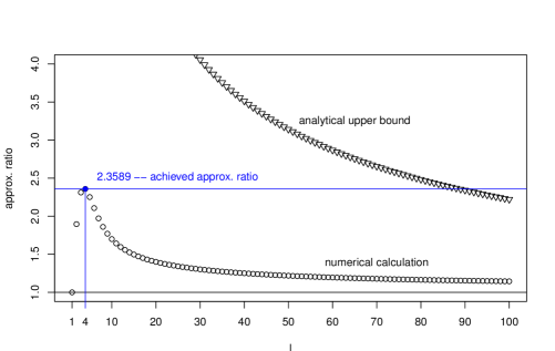
$\ell$	ratio
1	1
2	1.90
3	2.32
4	2.3589
5	2.26
6	2.11
7	1.98
8	1.86
9	1.78
10	1.70
11	1.65
12	1.60

Figure 6: The numerical and the analytical upper bound on the approximation ratio on intervals $(\ell-1,\ell)$, for each $\ell\in[k]$.

Appendix D Omitted Proofs from Section 3

Proof of Theorem 9.

We reduce an instance of Fault Tolerant $k$-median with Clients Multiplicities to an instance of Fault Tolerant $k$-median by replacing the multiple $m_{j}$ of a client $D_{j}$ with $m_{j}$ clients in the same location and with the same connectivity requirement (we will call such clients clones of $D_{j}$). Observe that there exists an optimal solution in which each clone of the same client is connected to the same set of open facilities. Next, we run the $93$-approximation algorithm of Hajiaghayi et al. [20] on such a constructed instance with clones. It is apparent that the solution that we obtain by following this procedure approximates the original instance with the ratio of 93. However, the issue is that $m_{j}$ can be exponential in the number of clients in the original instance, and so the most straightforward implementation of our reduction does not run in polynomial-time. To deal with that we will efficiently encode the reduced instance, and we will show that the algorithm of Hajiaghayi et al. can be adapted to run on such encoded instances. We proceed as follows.

First, we solve the LP part of the original algorithm [20] with the additional multiplicative factors $\{m_{j}\}_{D_{j}\in\mathcal{D}}$ added to the objective function. From the solution to the LP, $(y_{i})_{i\in[m]}$ with $\sum_{i=1}^{m}y_{i}=k$, we construct an optimal assignment of the clients to the facilities. We encode such an assignment efficiently by grouping all clones of the same client into a single cluster and storing an assignment for a single client for each cluster only (we call such a client the representative of the cluster). In particular, note that all clones in the same cluster have the same assignments and so, they all have the same average and maximal assignment costs. We use this property in the next step of the original algorithm: creating bundles of volume $1$ [20, Algorithm 1]. By a careful analysis of this algorithm we can observe that no new bundles are created for a cloned client (lines 5 and 6 of [20, Algorithm 1]) and so that the cloned clients can be considered in bunches.

Next, as in the original algorithm, we divide the clients into safe and dangerous by the criterion on the ratio of the maximal and the average cost in the assignment vector. Intuitively, if the maximum is much higher than the average then the client is marked as dangerous (for a formal definition see [20, Section 2.2]), otherwise it is considered safe. Hence, the clones of the same client are either all safe or all dangerous. In the latter case they are also in conflict: they are close and they have the same connectivity requirements (for a definition also see [20, Section 2.2]). Thus, in the filtering phase [20, Algorithm 2] either all the dangerous clones of the same client are filtered out or exactly one of them survives; without loss of generality we can assume that the representative of the cluster survives. In fact, this is the main reason why we can quite easy adapt the algorithm. The next step, that is building a laminar family [20, Algorithm 3], is independent on clients that were filtered out, and so it can be performed on our efficiently encoded instance. The safe clients are not used later on by the algorithm (they are only the side effect of creating bundles and later on they only appear in the algorithm’s analysis). Finally, the rounding process of the algorithm ([20, Section 2.3]) depends on the set of constructed bundles and on the set of filtered dangerous clients (and the induced laminar family), and as we discussed it is possible to construct each of the two families with efficient encoding. This completes the proof.

∎

Proof of Lemma 10.

Let $C$ be an $\alpha$-approximate solution to $I^{\prime}$. By ${\mathrm{FT\text{-}k\text{-}med\text{-}multi}}(C,j)$ we denote be the total cost of the clients $D_{j,1},D_{j,2},\dots,D_{j,k}$ constructed through reduction from Figure 3. Similarly, let ${\mathrm{OWA\text{-}k\text{-}med}}(C,j)$ be the cost of the client $D_{j}$ for $C$ in $I$. For each client $D_{j}$ we have:

$${\mathrm{FT\text{-}k\text{-}med\text{-}multi}}(C,j) =\sum_{r=1}^{k}m_{j,r}\cdot\left(\sum_{i=1}^{r}c_{i}^{\rightarrow}(C,j)\right)=\sum_{r=1}^{k}\sum_{i=1}^{r}m_{j,r}\cdot c_{i}^{\rightarrow}(C,j)$$

$$=\sum_{r=1}^{k}\sum_{i=1}^{r}m_{j,r}\cdot c_{i}^{\rightarrow}(C,j)=\sum_{i=1}^{k}\sum_{r=i}^{k}m_{j,r}\cdot c_{i}^{\rightarrow}(C,j)$$

$$=\sum_{i=1}^{k}\left(c_{i}^{\rightarrow}(C,j)\cdot\sum_{r=i}^{k}m_{j,r}\right)$$

$$=\sum_{i=1}^{k}c_{i}^{\rightarrow}(C,j)\cdot w_{i}\cdot Q=Q\cdot{\mathrm{OWA\text{-}k\text{-}med}}(C,j).$$

Let $C^{*}_{I}$ and $C^{*}_{I^{\prime}}$ be optimal solutions for $I$ and $I^{\prime}$, respectively. By the same reasoning, we have that:

$${\mathrm{FT\text{-}k\text{-}med\text{-}multi}}(C^{*}_{I},j)=Q\cdot{\mathrm{OWA\text{-}k\text{-}med}}(C^{*}_{I},j).$$

And, thus, that:

$$\sum_{D_{j}\in\mathcal{D}}{\mathrm{OWA\text{-}k\text{-}med}}(C,j)=\sum_{D_{j}\in\mathcal{D}}\frac{1}{Q}{\mathrm{FT\text{-}k\text{-}med\text{-}multi}}(C,j)$$

$$\leq\alpha\frac{1}{Q}\sum_{D_{j}\in\mathcal{D}}{\mathrm{FT\text{-}k\text{-}med\text{-}multi}}(C^{*}_{I^{\prime}},j)\leq\alpha\frac{1}{Q}\sum_{D_{j}\in\mathcal{D}}{\mathrm{FT\text{-}k\text{-}med\text{-}multi}}(C^{*}_{I},j)$$

$$=\alpha\sum_{D_{j}\in\mathcal{D}}{\mathrm{OWA\text{-}k\text{-}med}}(C^{*}_{I},j)\text{.}$$

This completes the proof. ∎

Appendix E Hardness of approximation

In the main text we have shown that the OWA $k$-median problem with the harmonic sequence of weights admits very good approximations. In this section we show that for many other natural sequences of weights, the considered problem is hard to approximate, unless we introduce additional assumptions, such as the assumptions that the costs satisfy the triangle inequality. Our hardness results hold already for 0/1 costs.

Let us start by considering the OWA $k$-median problem for a certain specific class of weights. For each $k\in{{\mathbb{N}}}$, let $w^{(k)}=\big{(}w^{(k)}_{1},\ldots,w^{(k)}_{k}\big{)}$ be a sequence of weights used in OWA $k$-median. Fix $\lambda\in(0,1)$. We say that the clients care only about the $\lambda$-fraction of facilities if for each $k$ it holds that $w^{(k)}_{i}=0$ whenever $i>\lambda k$. For instance, we say that the clients care only about 90% of facilities if the cost of each client from a set $C$ does not depend on the $10\%$ of worst facilities in $C$.

First, we prove a simple result which says that if there exists $\lambda$ such that the clients care only about the $\lambda$-fraction of facilities, and if the costs of clients from facilities can be arbitrary, in particular if they cannot be represented as distances satisfying the triangle inequality, then the problem does not admit any approximation.

Theorem 21.

Fix $\lambda\in(0,1)$ and consider the problem OWA $k$-median where clients care only about the $\lambda$-fraction of facilities. For any positive computable function $\alpha$, there exists no polynomial-time $\alpha$-approximation algorithm for OWA $k$-median, unless ${\mathsf{P}}={\mathsf{NP}}$.

Proof.

Let us fix a function $\alpha$ and for the sake of contradiction, let us assume that there exists a polynomial time $\alpha$-approximation algorithm $\mathcal{A}$ for OWA $k$-median. We will show that $\mathcal{A}$ can be used to find exact solutions to the exact set cover problem, X3C. This will stay in contradiction with the fact that X3C is ${\mathsf{NP}}$-hard [19].

Let $I$ be an instance of X3C, where we are given a set of $3n$ elements $E=\{e_{1},\ldots,e_{3n}\}$, and a collection $\mathcal{S}$ of subsets of $E$ such that each set in $\mathcal{S}$ contains exactly 3 elements from $E$. We ask if there exists a subcollection $C$ of $n$ subsets from $\mathcal{S}$ such that each element from $E$ belongs to exactly one set from $C$.

From $I$ we construct an instance of OWA $k$-median in the following way. First, we set the size of the committee $k=\left\lceil\frac{n}{1-\lambda}\right\rceil$. Let $p$ be the index of the last positive weight in the sequence $w^{(k)}$. Since clients care only about the $\lambda$-fraction of facilities, we know that $k-p>k-\lambda k\geq n$. Our set of facilities consists of three groups $\mathcal{F}=\mathcal{S}\cup H\cup H^{\prime}$, i.e., we have facilities which correspond to subsets from $\mathcal{S}$ and two groups of dummy facilities. We set $|H|=p-1$ and $|H^{\prime}|=k-n-p+1$. Our set of clients consist of two groups $\mathcal{D}=E\cup G$, where $G$ is the set of dummy clients with $|G|=|H^{\prime}|$. Let us now describe the preferences of clients over facilities. For each client $j\in\mathcal{F}$ and each dummy facility $i\in H$ we set $c_{i,j}=0$. Further, for each non-dummy client $j\in E$ and a non-dummy facility $i\in\mathcal{S}$ we set $c_{i,j}=0$ if and only if $j\in i$. Finally, we match dummy clients from $G$ with dummy facilities from $H^{\prime}$ so that each client is matched to exactly one facility and each facility to exactly one client, and set $c_{i,j}=0$ whenever $i$ and $j$ are matched. For all remaining pairs $(i,j)$ we set $c_{i,j}=1$.

Let $C^{*}$ be an optimal set of facilities. We will show that the total cost of clients from $C^{*}$ is 0 if and only if there exists an exact cover for our initial instance $I$.

$(\implies)$ Assume there exists an exact cover in $I$—let $C$ denote the collection of $n$ subsets covering all the elements. If we set $C^{*}=C\cup H\cup H^{\prime}$, then each client has exactly $p$ facilities with distance $0$. Note that $|C^{*}|=n+p-1+k-n-p+1=k$. For the remaining $k-p$ facilities the weights are equal to zero. Thus, the total cost of clients from $C^{*}$ is equal to 0.

$(\impliedby)$ Assume the total cost of clients from $C^{*}$ is equal to 0. In particular, the clients from $G$ need to have cost equal to $0$, so $H\cup H^{\prime}$ must be the part of a winning committee. Similarly, the remaining $n$ facilities must correspond to the cover of $E$.

If there exists a winning committee with the total cost of clients equal to 0, then algorithm $\mathcal{A}$ would find such committee. This completes the proof. ∎

Hence any approximation for OWA $k$-median can recognize whether the instance is YES-instance. Next, we prove a more specific hardness result for the $p$-geometric sequence of weights.

Theorem 22.

Consider the OWA $k$-median problem for the $p$-geometric sequence of weights. For each $c<1$, there exists no polynomial-time $(n^{-c\ln(p)-1})$-approximation algorithm for the problem unless ${\mathsf{P}}={\mathsf{NP}}$.

Proof.

Let us fix $c<c^{\prime}<1$. For the sake of contradiction, let us assume that there exists a polynomial-time $(n^{-c\ln(p)-1})$-approximation algorithm $\mathcal{A}$ for our problem. We will show that this algorithm can be used as an $c^{\prime}\ln(n)$-approximation algorithm for the Set Cover problem, which, unless ${\mathsf{P}}={\mathsf{NP}}$, will stay in contradiction with the approximation threshold established by Dinur et al. [12].

Let us take an instance $I$ of the Set Cover problem. In $I$ we are given a set of $n$ elements $E$, a collection $\mathcal{S}$ of subsets of $E$. We ask about minimal $k$ such that there is a subcollection $C$ of $k$ subsets from $\mathcal{S}$ such that each element from $E$ belongs to some set from $C$. Without loss of generality we can assume that $n$ is big enough to satisfy $c\ln(n)+1<c^{\prime}\ln(n)$.

From $I$ we construct an instance $I^{\prime}$ of OWA $k$-median as follows. We set $P=\sum_{i=1}^{k}p^{i-1}$ and $x=\lceil c\ln(n)+1\rceil$, thus $c\ln(n)+1\leq x\leq c^{\prime}\ln(n)$. For each element $e\in E$ we introduce one client. Further, for each set $S\in\mathcal{S}$ we introduce $x$ facilities $S_{1},\ldots,S_{x}$. The cost of a client $e$ for a facility $S_{i}$ is equal to 0 if and only if $e\in S$; otherwise, it is equal to one. Finally, we guess the optimal solution $k$ to $I$, and set the size of the desired set of facilities to $k_{\mathrm{fac}}=k\cdot x$.

Let us assume that there exist a set cover $C$ of size $k$ for the original instance $I$. What is the cost of the clients in the optimal solution for $I^{\prime}$? Let us consider the set of $k_{\mathrm{fac}}$ facilities $C^{\prime}$ constructed in the following way: for each set from the cover $S\in C$ we take all $x$ facilities that correspond to $S$ and add them to $C^{\prime}$. Observe that each client has cost equal to zero from at least $x$ facilities from $C^{\prime}$. Thus, the total cost of clients from $C^{\prime}$ is at most equal to (recall that $P=\sum_{i=1}^{K}p^{i-1}$):

$${w\mathrm{{}_{dis}}}(C^{\prime})=\sum_{j=1}^{n}{w\mathrm{{}_{dis}}}(C^{\prime},j) \leq n\big{(}p^{x}+p^{x+1}+\ldots+p^{K-1}\big{)}\leq$$

$$\leq n\big{(}p^{c\ln(n)+1}+p^{c\ln(n)+2}+\ldots+p^{K-1}\big{)}<np^{c\ln(n)}\cdot P=$$

$$=n\cdot e^{\ln(p)\cdot c\cdot\ln(n)}\cdot P=n\cdot n^{c\ln(p)}\cdot P=Pn^{c\ln(p)+1}\text{.}$$

Now, let us take the set of $k_{\mathrm{fac}}$ facilities $C^{\prime\prime}$ such that some client has cost equal to one from each facility from $C^{\prime\prime}$. Then, ${w\mathrm{{}_{dis}}}(C^{\prime\prime})\geq P$. Thus, an $(n^{-c\ln(p)-1})$-approximation algorithm for OWA $k$-median with the $p$-geometric sequence of weights needs to return a solution where each client has cost equal to zero from at least one facility. From such solution, however, we can extract at most $k_{\mathrm{fac}}$ sets which form a cover of the original instance. Thus, our algorithm $\mathcal{A}$ can be used to find $x$-approximation solutions for the Set Cover problem (recall that $x<c^{\prime}\ln(n)$), which is impossible under the standard complexity theory assumptions [12]. This completes the proof. ∎

Using that we obtain

Corollary 23.

There is no polynomial-time constant-factor approximation algorithm for the OWA $k$-median problem for the $p$-geometric sequence of weights when $p<\nicefrac{{1}}{{e}}$.

References

- [1] S. Ahmadian, A. Norouzi-Fard, O. Svensson, and J. Ward. Better guarantees for k-means and euclidean k-median by primal-dual algorithms. In Proceedings of the 58th IEEE Symposium on Foundations of Computer Science, pages 61–72, 2017.
- [2] N. Ailon, M. Charikar, and A. Newman. Aggregating inconsistent information: Ranking and clustering. Journal of the ACM, 55(5):23:1–23:27, 2008.
- [3] A. Auger and B. Doerr. Theory of randomized search heuristics: Foundations and recent developments. World Scientific Publishing, 2011.
- [4] H. Aziz, M. Brill, V. Conitzer, E. Elkind, R. Freeman, and T. Walsh. Justified representation in approval-based committee voting. Social Choice and Welfare, 48(2):461–485, 2017.
- [5] M. Brill, J-F. Laslier, and P. Skowron. Multiwinner approval rules as apportionment methods. In Proceedings of the 31st AAAI Conference on Artificial Intelligence, pages 414–420, 2017.
- [6] J. Byrka, T. Pensyl, B. Rybicki, A. Srinivasan, and K. Trinh. An improved approximation for k-median and positive correlation in budgeted optimization. ACM Transactions on Algorithms, 13(2):23:1–23:31, 2017.
- [7] I. Caragiannis, J. A. Covey, M. Feldman, C. M. Homan, C. Kaklamanis, N. Karanikolas, A. D. Procaccia, and J. S. Rosenschein. On the approximability of Dodgson and Young elections. Artificial Intelligence, 187:31–51, 2012.
- [8] I. Caragiannis, C. Kaklamanis, N. Karanikolas, and A. D. Procaccia. Socially desirable approximations for Dodgson’s voting rule. ACM Transactions on Algorithms, 10(2):6:1–6:28, 2014.
- [9] B. Chamberlin and P. Courant. Representative deliberations and representative decisions: Proportional representation and the Borda rule. American Political Science Review, 77(3):718–733, 1983.
- [10] D. Coppersmith, L. Fleischer, and A. Rudra. Ordering by weighted number of wins gives a good ranking for weighted tournaments. ACM Transactions on Algorithms, 6(3):55:1–55:13, 2010.
- [11] M. Cygan, Ł. Kowalik, A. Socała, and K. Sornat. Approximation and parameterized complexity of minimax approval voting. In Proceedings of the 31st AAAI Conference on Artificial Intelligence, pages 459–465, 2017.
- [12] I. Dinur and D. Steurer. Analytical approach to parallel repetition. In Proceedings of the 46th ACM Symposium on Theory of Computing, pages 624–633, 2014.
- [13] D. P. Dubhashi, J.Jonasson, and D. Ranjan. Positive influence and negative dependence. Combinatorics, Probability and Computing, 16(1):29–41, 2007.
- [14] C. Dwork, R. Kumar, M. Naor, and D. Sivakumar. Rank aggregation methods for the web. In Proceedings of the 10th International World Wide Web Conference, pages 613–622, 2001.
- [15] E. Elkind, P. Faliszewski, P. Skowron, and A.i Slinko. Properties of multiwinner voting rules. Social Choice and Welfare, 48(3):599–632, 2017.
- [16] P. Faliszewski, E. Hemaspaandra, and L. A. Hemaspaandra. Multimode control attacks on elections. Journal of Artificial Intelligence Research, 40:305–351, 2011.
- [17] P. Faliszewski, J. Sawicki, R. Schaefer, and M. Smolka. Multiwinner voting in genetic algorithms for solving ill-posed global optimization problems. In Proceedings of the 19th International Conference on the Applications of Evolutionary Computation, pages 409–424, 2016.
- [18] R. Gandhi, S. Khuller, S. Parthasarathy, and A. Srinivasan. Dependent rounding and its applications to approximation algorithms. Journal of the ACM, 53(3):324–360, 2006.
- [19] M. R. Garey and D. S. Johnson. Computers and Intractability: A Guide to the Theory of NP-Completeness. W. H. Freeman, 1979.
- [20] M. T. Hajiaghayi, W. Hu, J. Li, S. Li, and B. Saha. A constant factor approximation algorithm for fault-tolerant k-median. ACM Transactions on Algorithms, 12(3):36:1–36:19, 2016.
- [21] D.S. Hochbaum and D.B. Shmoys. A best possible heuristic for the k-center problem. Mathematics of Operations Research, 10(2):180–184, 1985.
- [22] C. M. Homan and L. A. Hemaspaandra. Guarantees for the success frequency of an algorithm for finding Dodgson-election winners. Journal of Heuristics, 15(4):403–423, 2009.
- [23] K. Joag-Dev and F. Proschan. Negative association of random variables with applications. The Annals of Statistics, 11(1):286–295, 1983.
- [24] C. Kenyon-Mathieu and W. Schudy. How to rank with few errors. In Proceedings of the 39th ACM Symposium on Theory of Computing, pages 95–103, 2007.
- [25] D. Kilgour. Approval balloting for multi-winner elections. In J. Laslier and R. Sanver, editors, Handbook on Approval Voting, pages 105–124. Springer, 2010.
- [26] J. M. Kleinberg, C. H. Papadimitriou, and P. Raghavan. Segmentation problems. Journal of the ACM, 51(2):263–280, 2004.
- [27] J. B. Kramer, J. Cutler, and A. J. Radcliffe. Negative dependence and Srinivasan’s sampling process. Combinatorics, Probability and Computing, 20(3):347–361, 2011.
- [28] T. Lu and C. Boutilier. Budgeted social choice: From consensus to personalized decision making. In Proceedings of the 22nd International Joint Conference on Artificial Intelligence, pages 280–286, 2011.
- [29] T. Lu and C. Boutilier. Value-directed compression of large-scale assignment problems. In Proceedings of the 29th AAAI Conference on Artificial Intelligence, pages 1182–1190, 2015.
- [30] J. C. McCabe-Dansted, G. Pritchard, and A. M. Slinko. Approximability of dodgson’s rule. Social Choice and Welfare, 31(2):311–330, 2008.
- [31] B. Monroe. Fully proportional representation. American Political Science Review, 89(4):925–940, 1995.
- [32] P. Skowron, P. Faliszewski, and J. Lang. Finding a collective set of items: From proportional multirepresentation to group recommendation. Artificial Intelligence, 241:191–216, 2016.
- [33] P. Skowron, P. Faliszewski, and A. M. Slinko. Achieving fully proportional representation: Approximability results. Artificial Intelligence, 222:67–103, 2015.
- [34] A. Srinivasan. Distributions on level-sets with applications to approximation algorithms. In Proceedings of the 42nd IEEE Symposium on Foundations of Computer Science, pages 588–597, 2001.
- [35] C. Swamy and D.B. Shmoys. Fault-tolerant facility location. ACM Transactions on Algorithms, 4(4):51:1–51:27, 2008.
- [36] T. N. Thiele. Om flerfoldsvalg. In Oversigt over det Kongelige Danske Videnskabernes Selskabs Forhandlinger, pages 415–441. 1895.
- [37] R. R. Yager. On ordered weighted averaging aggregation operators in multicriteria decisionmaking. IEEE Trans. Systems, Man, and Cybernetics, 18(1):183–190, 1988.