A Graphical method for simplifying Bayesian Games

Abstract

If the influence diagram (ID) depicting a Bayesian game is common knowledge to its players then additional assumptions may allow the players to make use of its embodied irrelevance statements. They can then use these to discover a simpler game which still embodies both their optimal decision policies. However the impact of this result has been rather limited because many common Bayesian games do not exhibit sufficient symmetry to be fully and efficiently represented by an ID. The tree-based chain event graph (CEG) has been developed specifically for such asymmetric problems. By using these graphs rational players can make analogous deductions, assuming the topology of the CEG as common knowledge. In this paper we describe these powerful new techniques and illustrate them through an example modelling a game played between a government department and the provider of a website designed to radicalise vulnerable people.

Keywords: Adversarial risk; Bayesian game theory; chain event graph; decision tree; influence diagram; parsimony

1 Introduction

There are two principal conceptual difficulties in applying results from Bayesian game theory in a number of domains. Firstly, whilst it might be plausible for a player to know the broad structure of an opponent’s utility function when that opponent is subjective expected utility maximizing (SEUM), for a player to also believe that she knows the exact quantitative form of that utility function or the precise formulation of the distribution of its attributes is less plausible. Secondly, as for example [15] has pointed out, however compelling our beliefs are that an opponent’s rationality should induce her to be SEUM, in practice most people simply are not. So any application of a theory which starts with this assumption is hazardous. These issues induced [13] to suggest giving up on the rationality hypothesis entirely and instead modelling the opponent simply in terms of her past behaviour.

However others have perservered with rationality modelling by addressing these real modelling challenges more qualitatively. For example [24] suggested a way to address the first difficulty described above. We can continue to model successfully provided that the conditional independences associated with various hypotheses and the attributes of each player’s utility function are common knowledge, but we do not need that the players know the quantitative forms of others’ inputs. This framework developed from methods for simplifying influence diagrams (IDs) [10, 28], described first in [19] and then [23]. When players are all SEUM, substantive conclusions can sometimes be made concerning those aspects of the problem upon which a rational opponent’s decision rules might depend. This in turn allows players to determine ever simpler forms for their own optimal decision rules. So models can be built which at least respect some of the structural implications of rationality hypotheses before being embellished with further structure gleaned from behavioural data, or the bold assumption that an opponent’s quantitative preferences and beliefs can be fully quantified by everyone. Even the second criticism of a Bayesian approach outlined above is at least partially addressed, since the methods need only certain structural implications of SEUM to be valid, not that all players are SEUM.

In this way game theory can therefore be used not to fully specify the quantitative form of a competitive domain but simply to provide hypotheses about the likely dependence structure that rationality assumptions might imply for such models. These models can then be embellished with further historical quantitative information using the conventional Bayesian paradigm.

It has been possible to demonstrate the efficacy of the approach when modelling certain rather domain-specific applications, but it has proved rather limited in scope [24, 26]. One problem is that the structure of many games cannot be fully and effectively represented by an ID (see for example [4, 5, 17]). Usually the underlying game tree is highly asymmetric and so the symmetries necessary for an encompassing and parsimonious ID representation of the game are not present. This is one characteristic of the types of games that we consider in this paper; we discuss other important attributes in the following paragraphs.

Harsanyi [9] considered games where the players are uncertain about some or all of the following – the other players’ utility functions, the strategies available to the other players, and the information other players have about the game. In the games considered in this paper each player holds a body of common knowledge – the exact form of other players’ utility functions is unknown, but the variables these functions depend upon (a feature of the conditional independence structure of the game) are known; the strategies available to the other players are known; and what information is known to the other players is also known. So essentially the games we consider are ones where the “structure” is common knowledge, but the exact values of other players’ utilities and the probability distributions of some chance variables are not.

In contrast to Harsanyi, Banks et al in [1] state that Game theory needs the defenders to know the attackers’ utilities and probabilities, and the attackers to know the defenders’ utilities and probabilities, and for both to know that these are common knowledge. We do not agree that these are absolute requirements, but it is certainly true that a player cannot solve a game to her satisfaction unless she has some values for her opponents’ utilities and probabilities. So in our games, players assign subjective probabilities to their unknowns and estimate values of their opponents’ utility functions. Each player’s utilities depend not only on the strategies chosen by the various players, but also on chance.

We take a decision-theoretic approach to Bayesian Game theory. Our games are sequential (typically with players acting alternately, and with chance variables interspersed between the players’ actions). The standard description for such a game is Extensive Form Bayesian Game with Chance moves; they are generally expressed as a game tree (or as an ID [24] or MAID – multi-agent influence diagram [14]).

Asymmetric games, as described above, are being played with increasing frequency wherever large constitutional organisations (governments, police forces etc.) are at risk from or attempting to combat criminal or anticonstitutional organisations or networks. An example is described below, taken from this area, probably less familiar than games in a commercial context.

Governments and police play a game with groups trying to influence or radicalise susceptible individuals. These radicalisers often attempt to influence vulnerable people via the web. The government strategy here can be thought of as a combination of prevention and pursuit: if a website is easily accessible then it might be best just to shut it down; if it is difficult to access, then perhaps it is better to monitor, collect information and then act to scare vulnerable people sufficiently so that they do not get involved with any anticonstitutional group. But when should the government act? There is a trade-off here between frustrating a number of attempts to radicalise vulnerable people, and bringing down a whole anticonstitutional group (with the attached risks of failure and of exposing more susceptible individuals to malign influence for a longer period of time). The decisions available to the radicalisers are similar; the asymmetry of the game arises from the fact that different decisions by both players lead to very different collections of possible futures.

The Chain Event Graph (CEG) was introduced in 2008 [27] for the modelling of probabilistic problems whose underlying trees exhibit a high degree of asymmetry. It provides a platform from which to deduce dependence relationships between variables directly from the graph’s topology. CEGs have principally been used for learning/model selection (see for example [21, 2]), but also in two areas of interest to us in this paper – causal analysis (see for example [30, 7]), and also decision analysis [29] where the semantics of the CEG can be extended to provide algorithms which allow users to discover minimal sets of variables needed to fully specify an SEUM decision rule. In 2015 it was realised that CEGs include Acyclic Probabilistic Finite Automata (APFAs) as a special case [8].

In this paper we demonstrate how it is often possible to use causal CEGs to deduce (from appropriate qualitative assumptions) a simpler representation of a two person game. To retain plausibility we assume only the qualitative structure of the problem (as expressed by the topology of a CEG) is common knowledge, and that the players are SEUM given the information available to them when they make a move. In section 2 we introduce the semantics of the decision CEG and discuss the principle of parsimony. To illustrate how the CEG can be used for the representation and analysis of games, and also how it can be used to simplify these games, section 3 contains a description of a 2 player game modelling a simplified version of the radicalisation scenario described above. Section 4 contains a discussion of ideas prompted by the work in earlier sections.

We have focussed here on two person adversarial games. However, similar techniques can be used both for non-adversarial games and also for multi-player games. We have also assumed here that we are supporting one of the two players, but note that because of the common knowledge assumption we have made, the qualitative results of the analysis are equally valid to this player’s opponent or indeed some independent external observer.

2 Decision Chain Event Graphs

2.1 Conditional independence, Chain Event Graphs and causal hypotheses

Bayesian Networks (BNs) and Influence Diagrams express the conditional independence/Markov structure of a model through the presence/absence of edges between vertices of the graph. We say that a variable $X$ is independent of a variable $Y$ given $Z$ (written $X\amalg Y\ |\ Z$) if once we know the value taken by $Z$, then $Y$ gives us no further information for forecasting $X$. The structure of an ID can be used to produce fast algorithms for finding optimal decision strategies [19].

One advantage that CEGs have over BNs and IDs for asymmetric problems is that they can be used to represent context-specific conditional independence properties such as $X\amalg Y\ |\ (Z=z)$, which hold only for a subset of values of the conditioning variable.

The CEG is a function of a probability (or event) tree, having the same structure as a game tree, but with all non-leaf vertices being chance and all edges representing outcomes of these chance nodes, rather than actions of a player, We introduce two partitions of the vertices of the tree:

• Vertices in the same stage have sets of outgoing edges representing the same collections of possible outcomes, and have the same probabilities of these outcomes.

• Vertices in the same position have sets of outgoing subpaths representing the same collections of possible complete futures, and have the same probabilities of these futures.

These equivalence classes encode (context-specific) conditional independences as follows: Given arrival at one of the vertices in a particular stage, the next development is independent of precisely which vertex has been arrived at. Given arrival at one of the vertices in a particular position, the complete future is independent of precisely which vertex has been arrived at.

Our CEG is then produced from the tree by combining (or coalescing) vertices which are in the same position. Vertices in the same stage are generally given the same colour, and equivalent edges emanating from vertices in the same stage are generally also given the same colour. The stages and positions between them encode the full conditional independence/Markov structure of our model. More detailed definitions are given in [27].

In [16], Pearl discusses the assumptions under which BNs can be considered causal (a more decision-theoretic approach to graphical modelling is considered in [25]). We have shown that under similar assumptions CEGs can also be considered as causal [30]. Heuristically this means that the model specified by a CEG continues to be valid when particular variables are manipulated. Such a hypothesis is a particularly natural one to entertain in decision problems, where a decision maker (DM) by choosing a specific action at some point can be thought of as manipulating a specific variable. The hypothesis is also a natural one to entertain in a game whose underlying structure is common knowledge and where each player is able to manipulate their own decisions to a particular value, but nature or the player’s opponents will determine the value of other variables.

Those vertices in a CEG which we allow to be manipulated can be construed as decision nodes and the CEG as a function of a decision tree [28]. The remaining vertices in the CEG are then chance or utility nodes. In this mode the CEG is an elegant answer to the problems highlighted in [22, 17, 5, 4], where different actions can result in different choices in the future. As such it provides an alternative to valuation networks [20], decision circuits [3], sequential decision diagrams [6] and sequential IDs [12]. A full discussion of why IDs (including those supplemented by trees or similar) are unsatisfactory for the representation and analysis of asymmetric problems can be found in [4]. A brief comparison of decision CEGs with IDs, and with valuation networks, decision circuits, sequential decision diagrams and sequential IDs can be found in [29]. A more detailed comparison will soon be available in an extended version of this paper.

In [30] we were concerned primarily with the effects of a manipulation and whether these effects could be gauged from probabilities in the idle system. Considering the CEG as a function of a decision tree in contrast, we assume that the owner of the CEG has a utility function over the possible outcomes of the problem, and can then use techniques analogous to those used for decision trees to find an optimal decision rule for the decision maker. An introduction to the use of CEGs for decision analysis can be found in [29].

2.2 An example of how CEGs can be used to represent decision problems

Figures 1 and 2 illustrate how a decision tree is converted into a CEG. Figure 1 shows a variation of the Oil drilling example from [18]. A more detailed version of this example appears in [29].

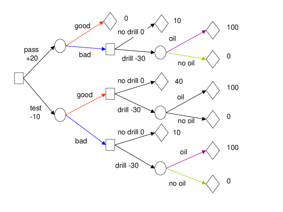
Figure 1: Coloured decision tree for Oil drilling example

We have an option on testing some ground for oil. We can either take up this option, at a cost of 10, or pass it on to another prospector for a fee of 20. Whoever does the testing, the outcomes are good or bad, with probabilities independent of who does the testing. If we have passed on the testing and the test result is good then we lose the option for drilling and get nothing. If it is bad then the other prospector will not drill and the option for drilling reverts to us. If we do the test and the result is good, then we can either drill, for a cost of 30, or sell the drilling rights for a fee of 40. If the result is bad, then regardless of who does the test, we can either drill ourselves, again for a cost of 30, or sell the drilling option for a fee of 10. If we drill and find oil we gain 100.

Decision nodes are indicated by squares, chance nodes by circles and utility nodes by diamonds. Utilities here are decomposed and appear both on the leaf utility nodes and on the edges emanating from decision nodes. Edges emanating from chance nodes have been assigned the same colour if the nodes are in the same stage, and if the edges represent the same outcome and carry the same probability. So for example the two good/bad chance nodes are in the same stage. Also the first and third drill/no drill decision nodes are in the same position, since they root subtrees which are identical in both topology and colouring.

In purely-probabilistic CEGs we usually combine all leaf nodes into a single sink node. With decision CEGs it is preferable to retain a number of leaf utility nodes, each representing a different final reward. The CEG corresponding to Figure 1 is given in Figure 2. The CEG is Extensive Form – that is the variables appear in the order that they appear to the DM. If there is oil in the ground it will have been there before we test or drill, but we don’t know this until we drill.

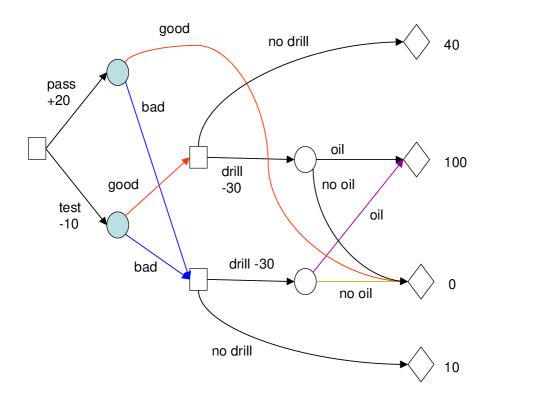
Figure 2: Decision CEG for Oil drilling example

As with purely-probabilistic CEGs, the colouring and coalescence in the decision CEG allow it to express the complete conditional independence/Markov structure of a problem through its topology [29]. If vertices are in the same stage then we know that the possible immediate future developments from these vertices are the same, and (if the vertices are chance nodes) that the probability of any specific immediate future development is the same. Vertices in the tree which are in the same position are combined in the decision CEG because the sets of possible complete future developments from these vertices are the same and have the same probability distribution.

In Figure 2 we have coloured the chance nodes which are in the same stage, and the edges emanating from them (indicating that they have the same probabilities). We have retained the colouring of the edges leaving the 2nd oil chance node to illustrate how these edges relate to those in Figure 1.

2.3 Parsimony

In the example above we have a single DM. When we move into games with more than one player, the CEG represents the problem to each of the players and its topology can be considered as common knowledge (CK). The underlying structure is causal to each player, but each decision node can only be manipulated by a single (specified) player. In [24] we considered IDs which obeyed the same assumptions as those described immediately above. Such IDs were resurrected and modified by [14] and called MAIDs (multi-agent influence diagrams). In [23] we noted that such IDs could be seen from the point of view of an informed observer to whom all nodes could be considered as chance nodes – a scenario which for example would be valid if the observer’s BN were causal and common knowledge.

The paper [24] describes how to produce a parsimonious representation of a game. When a player needs to make a decision at $D$, some of the information they have obtained beforehand may be superfluous for the purposes of making this decision. We then write

$$U\amalg Q^{S}(D)\ |\ (D,Q^{R}(D))$$ (1)

where $U$ is the utility for that player, and $Q(D)=\{Q^{S}(D),Q^{R}(D)\}$ ($S=$ superfluous, $R=$ required) is a partition of the information obtained by the player before making the decision (equivalent to the vertices in the ID with edges directed into $D$). In this case the player need only consider the configuration of the variables $Q^{R}(D)$ when choosing a decision at $D$ to maximise $U$. In [14] the authors use similar ideas which they call strategic relevance and s-reachability. Conditional independence statements involving decision variables and utilities are discussed in some detail in [29]. If the symmetry property of such statements is abandoned and a statement such as $X\amalg Y\ |\ Z$ is read only as $X$ is independent of $Y$ given $Z$, then statements involving decision variables and utilities are unambiguous providing they do not take the form $D\amalg\dots\ |\ \dots$, where $D$ is a decision variable; and if the statement involves a utility $U$ then it must be of the form $U\amalg\dots\ |\ \dots$.

3 CEGs for Games, and an example of a 2 player game

In section 3.1 we introduce an example of a 2 player adversarial game, which we will use to illustrate how CEGs can be used to represent and analyse such games. The ID of this example (Figure 3) appeared originally in [24] where it was used to demonstrate how the parsimony assumption can simplify the analysis required in a 2 player game. The problem is presented here within the context of a test of strength between a government department and a radicalising website provider. In section 3.3 we demonstrate that the idea of parsimony can be used to simplify CEG-based analysis; we also show how CEG methods accomodate problem asymmetry in their topology in a way that IDs do not. Moreover we see how the process of simplification can be directly linked to the asymmetries exhibited in the associated game tree.

3.1 Example: description and ID

In our example the players are the provider ($A$) of an internet site aimed at radicalising vulnerable people, and a government department (or police force) tasked with combatting radicalisation ($B$). The site provider has contacts with a radical group (RG); the government department is aware of this group, but has no wish to tackle them directly at the present time. Our example is a simplification of the real games being played, and combines aspects of both prevention and pursuit to illustrate how such games may develop. The example is concerned also with a single vulnerable person (VP). As already noted, we could adapt the methods described below to games with more than two players, but here, for simplicity, the behaviour of VP and RG are considered to be governed by chance.

The ID contains chance and decision nodes as described below. We assume here that we are supporting one player. In the description which follows, there is a utility pair associated with the chance variables $X_{3}$ and $X_{4}$, one of whose entries records our supported player’s utilities, and the other entry our supported player’s estimated values for their opponent’s utilities. For illustrative purposes, let our supported player be $A$ (!), so the 2nd entry in our utility pairs is $A$’s estimate of $B$’s utility. In Figure 3, and in the CEGs in Figures 4 to 7, we have outlined $A$’s decision nodes in red, and $B$’s decision nodes in blue, for ease of reading.

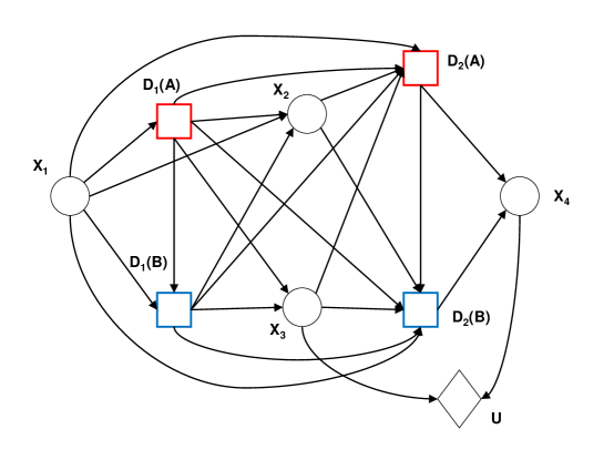
Figure 3: Initial ID

• VP visits the website and either posts to the site, or contacts RG via a link on the site. Both $B$ & $A$ observe VP’s action.

• $A$ decides either to contact VP, or to contact RG. $B$ observes $A$’s action.

• $B$ decides either to contact VP via the site in the guise of an RG-sympathiser, or to shut the site down. $A$ observes $B$’s action.

• $B$’s action at $D_{1}(B)$ may warn VP that he is being observed. The probability of this depends on whether VP posted to the site or contacted RG, on whether $A$ contacted VP at $D_{1}(A)$ or not, and on $B$’s action at $D_{1}(B)$. VP’s online behaviour indicating whether he is aware of being observed is itself observed by both $A$ & $B$.

• $A$’s action at $D_{1}(A)$ and $B$’s action at $D_{1}(B)$ either persuades RG to cut contact with $A$ (with utility pair $(U_{A},U_{B})=(-10,+10)$), or to increase their cooperation (with utility pair $(U_{A},U_{B})=(+10,0)$). The respective probabilities depend on which combination of $A$’s & $B$’s actions occurred. Behaviour of RG observed by both $A$ & $B$.

• $A$ posts to own site either pretending to be VP, or in the guise of a sympathiser. This post provides false information about themselves and their relationships with RG & VP. VP knows that he did not post the message and that the aspect of the information concerning his relationship with $A$ is false. The post is seen by $B$.

• $B$ decides either to arrest VP or not.

• VP either tells $B$ that the information is false, or does not. The probability of VP doing this depends on $A$’s action at $D_{2}(A)$ and $B$’s action at $D_{2}(B)$.

CEGs were designed for use with asymmetric problems. ID-representations often obscure such asymmetries and so even if a problem is expressed as an ID it might still incorporate significant numbers of hidden asymmetries. A decision CEG can depict explicitly any number of asymmetries, but for illustrative convenience we concentrate here on just one such possibility:

• If at $X_{3}$, RG cut contact, then $A$ believes that $B$ believes that the information is false ($(U_{A},U_{B})=(0,0)$) irrespective of what VP tells $B$. If at $X_{3}$, RG increased cooperation, then $A$ believes that $B$ believes that the information is true ($(U_{A},U_{B})=(+20,+10)$) if VP does not tell $B$ that it is false, and believes that it is false ($(U_{A},U_{B})=(0,0)$) if VP tells $B$ it is false.

Note that $A$’s estimate of $B$’s utility for ($X_{3}$: RG increased cooperation, $X_{4}$: VP does not tell $B$ that information is false) is positive because $A$ believes that $B$ believes the information. $U_{A}$ is large for this scenario because $A$ believes that they have successfully planted false information on $B$. If RG cuts contact at $X_{3}$ then the decisions made at $D_{2}(A),D_{2}(B)$ have no influence on $(U_{A},U_{B})$, and neither does the outcome of $X_{4}$.

Table 1: $(U_{A},U_{B})$ as a function of $X_{3}$ and $X_{4}$

		$X_{4}$: VP tells $B$ that false	VP does not …
$X_{3}$:	RG cuts contact	(-10, +10)	(-10, +10)
	RG increases …	(+10, 0)	(+30, +10)

We describe in sections 3.2 and 3.3 how this information can be incorporated directly into the topology of the CEG.

3.2 CEG and conditional independence structure

CEGs used for game analysis have the same relationship to game trees as Decision CEGs have to decision trees. In our CEG in Figure 4 there are no utilities on edges; they have been restricted to the terminal utility nodes (we have elsewhere described this as a Type 2 decision CEG [29]). For each utility node, each player has an associated utility pair (as described in section 3.1). From the player’s perspective, one value in the pair corresponds to their own utility value for this outcome, whereas the other corresponds to the player’s estimate of their opponent’s utility value for this outcome. We maintain that the CEG in Figure 4 is causal, and that its topology is common knowledge.

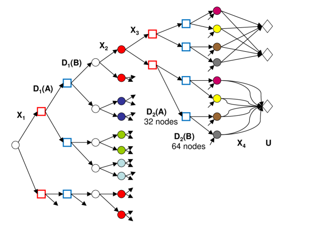
Figure 4: Naive CEG of model depicted in Figure 3

We have given vertices in the same stage the same colour (as in Figure 2), but have not coloured emanating edges to avoid cluttering the diagrams. We can read the colouring as, for example the probability that $X_{3}=1$ given the histories up to each red $X_{3}$ vertex is the same, but different from that given the histories up to any of the differently coloured $X_{3}$ vertices.

For illustrative convenience the CEG has been drawn out in more detail than is strictly necessary. The diagram need really only show certain key aspects of the model – the colouring of the $X_{3}$ vertices; the grouping and colouring of the $X_{4}$ vertices; and the asymmetric grouping of the utility nodes (reflecting the utilities given in Table 1). These four aspects correspond to the four non-trivial conditional independence statements associated with the model. So the full CEG need never be drawn out – it can simply be stored as a collection of computer constraints. The players need the picture only as a reminder of the key local properties and asymmetric aspects of the game.

Various conditional independence/Markov properties can be read off CEGs by considering individual positions, stages or cuts through these. Stages encode statements about the immediate future, whereas positions encode statements about the complete future.

If we consider a cut through the 16 $X_{3}$ vertices, we see that they are grouped into four stages. So for instance the 1st, 2nd, 9th & 10th $X_{3}$ vertices are in the same stage – the probability that $X_{3}=1$ (say) is the same for the four histories $X_{1}=1\ \hbox{or}\ 2,D_{1}(A)=1,D_{1}(B)=1,X_{2}=1\ \hbox{or}\ 2$. Similar results hold for the other groups of vertices, and together give us the property that

$$X_{3}\amalg(X_{1},X_{2})\ |\ (D_{1}(A),D_{1}(B)).$$

This property concerns $X_{3}$, but not $D_{2}(A),D_{2}(B),X_{4}$ or $U$. It can also of course be read from the ID in Figure 3. Similarly we see that the $X_{4}$ vertices are also grouped into four stages, and a similar reading of the stage cut through these vertices gives us the property

$$X_{4}\amalg(X_{1},D_{1}(A),D_{1}(B),X_{2},X_{3})\ |\ (D_{2}(A),D_{2}(B)).$$

There are 8 $X_{4}$ vertices (although 4 stages, and in the underlying tree 128 vertices) because the utility function depends on the value taken by $X_{4}$ but also on the value taken by $X_{3}$ (which has no direct influence on $X_{4}$).

When considering position cuts we ignore the colouring and groupings into stages. The first $X_{4}$ vertex corresponds to the histories $X_{1}=1\ \hbox{or}\ 2,\break D_{1}(A)=1\ \hbox{or}\ 2,D_{1}(B)=1\ \hbox{or}\ 2,X_{2}=1\ \hbox{or}\ 2,X_{3}=1,D_{2}(A)=1,D_{2}(B)=1$. So reading the position cut through the $X_{4}$ vertices gives us the property

$$(X_{4},U)\amalg(X_{1},D_{1}(A),D_{1}(B),X_{2})\ |\ (X_{3},D_{2}(A),D_{2}(B)).$$ (2)

Here the property concerns $X_{4}$, but also $U$, since positions encode statements about the complete future. We finally consider a cut through the utility nodes, and see that

$$U\amalg(X_{1},D_{1}(A),D_{1}(B),X_{2},D_{2}(A),D_{2}(B))\ |\ (X_{3},X_{4}).$$

Our experience suggests that with practice, users of CEGs quickly become adept at the reading of the graphs for their conditional independence structure.

3.3 Simplifying the CEG

We now turn our attention to how parsimony allows us to simplify analysis. For a multi-player adversarial game, simplification takes the form of an iterative process whose steps are of two types – decision node coalescence, and barren node deletion. The process is run from leaf nodes to root node.

Decision node coalescence: As already noted, for a player making a decision at $D$, if she can learn that $U\amalg Q^{S}(D)\ |\ (D,Q^{R}(D))$, then she need only consider the configuration of the variables $Q^{R}(D)$ when choosing a decision at $D$ to maximise her utility. If $Q^{S}(D)$ is non-empty then in the CEG there are distinct decision nodes that are actually in the same position and therefore can be combined [29]. Two or more decision nodes (in a Type 2 decision CEG) are in the same position if:

• the subCEGs rooted in these nodes have the same topology,

• equivalent edges in these subCEGs have the same labels and (where appropriate) probabilities,

• equivalent branches in these subCEGs terminate in the same utility node.

Barren node deletion: As with IDs [19], decision CEGs may have barren nodes which can be deleted. A barren node in a Type 2 decision CEG [29] is simply a vertex all of whose emanating edges terminate in the same node. If the vertex is a decision node then whatever decision the DM makes is irrelevant, and if it is a chance node then whatever outcome happens is of no consequence. The deletion step proceeds as follows [29]:

If $w$ has only one child node then

• label this node $w_{\succ}$,

• for each node $w_{\prec}$ in the parent set of $w$: replace all edges $e(w_{\prec},w)$ by a single edge $e(w_{\prec},w_{\succ})$, and delete all edges $e(w,w_{\succ})$ and the node $w$.

We have noted that this simplification process works for adversarial games with two or more players. We expect that it will also work, possibly with some minor modification, for non-adversarial games as well.

With these tools at our disposal we can start to simplify the CEG from Figure 4.

The 5th to 8th $X_{4}$ nodes in Figure 4 are barren, as all their emanating edges terminate in the same utility node. They can be deleted, and the edges entering them from $D_{2}(B)$ vertices extended so that they now terminate at the third utility node. But these $D_{2}(B)$ nodes are now also barren, as all their emanating edges now terminate in the same utility node. They can be deleted, and the edges entering them from $D_{2}(A)$ vertices extended so that they now terminate at the third utility node. These $D_{2}(A)$ nodes are now also barren, and once we have deleted them we get a reduced graph as in Figure 5.

Figure 5: First reduced CEG

Now considering the remainder of the graph, we can deduce from expression (2) that

$$U_{B}\amalg(X_{1},D_{1}(A),D_{1}(B),X_{2})\ |\ (D_{2}(B),X_{3}=1,D_{2}(A)).$$ (3)

So $Q^{S}(D_{2}(B))=\{X_{1},D_{1}(A),D_{1}(B),X_{2}\}$, and these variables can be considered as non-parents of $D_{2}(B)$ for the purposes of optimal decision making. The 32 remaining $D_{2}(B)$ vertices are grouped into two positions (corresponding to the combinations $X_{3}=1,D_{2}(A)=1\ \hbox{or}\ 2$), and we can combine these $D_{2}(B)$ vertices into two, each with 16 incoming edges corresponding to the 16 possible configurations of $(X_{1},D_{1}(A),D_{1}(B),X_{2})$. Each remaining $X_{4}$ vertex now has only 1 incoming edge.

A position cut through the $D_{2}(B)$ nodes now yields the statement

$$(D_{2}(B),X_{4},U)\amalg(X_{1},D_{1}(A),D_{1}(B),X_{2})\ |\ (X_{3}=1,D_{2}(A)),$$

which if viewed from the perspective of $B$ is an invalid statement – $B$ can choose arbitrarily between two actions at $D_{2}(B)$, so the statement that $D_{2}(B)$ is conditionally independent of other variables is nonsensical (see comment in section 2.3).

Figure 6: Second reduced CEG

However, this is a 2 player game, and at this point in the analysis we are considering the possible actions of $A$ at $D_{2}(A)$. To $A$ the behaviour of $B$ can be considered as random (or at least $D_{2}(B)$ can be considered as a chance variable), and so to $A$ the statement has meaning. We can therefore deduce that

$$U_{A}\amalg(X_{1},D_{1}(A),D_{1}(B),X_{2})\ |\ (D_{2}(A),X_{3}=1).$$

So $Q^{S}(D_{2}(A))=\{X_{1},D_{1}(A),D_{1}(B),X_{2}\}$, and these variables can be considered as non-parents of $D_{2}(A)$ for the purposes of optimal decision making. The 16 remaining $D_{2}(A)$ vertices are all in the same position (corresponding to $X_{3}=1$), and we can combine these $D_{2}(A)$ vertices into one, with 16 incoming edges corresponding to the 16 possible configurations of $(X_{1},D_{1}(A),D_{1}(B),X_{2})$. The two remaining $D_{2}(B)$ vertices now each have only 1 incoming edge. The resulting graph is given in Figure 6, where the redundant colouring of the remaining $X_{4}$ vertices has been removed.

We cover the remainder of the simplification process more rapidly. The 1st, 2nd, 9th & 10th $X_{3}$ vertices root identical subCEGs, so they are now in the same position and can be combined. The same is true of the other sets of coloured $X_{3}$ vertices. The 8 $X_{2}$ nodes are barren and can be deleted (we run the edges from the 4 $D_{1}(B)$ vertices straight into the appropriate $X_{3}$ vertices). The 1st & 3rd $D_{1}(B)$ vertices now root identical subCEGs so are in the same position. The same is true of the 2nd & 4th $D_{1}(B)$ vertices, and the two $D_{1}(A)$ vertices. Finally, the $X_{1}$ node is now barren so can be removed, giving us the parsimonious CEG in Figure 7.

Figure 7: Parsimonious CEG

At this point it is worth reminding ourselves that we are supporting one player, here $A$, so even when we have considered $U_{B}$ (as in expression (3)), we have been looking at the game from $A$’s perspective. Now, both players start with the same initial CEG (Figure 4) since its topology is considered to be common knowledge; and some aspects of the simplification process will occur regardless of which player’s shoulder we are looking over (such as the removal of the vertices associated with $X_{1}$ and $X_{2}$). But other aspects of the simplification might be different for $B$, since the process will depend on $B$’s own utilities and on $B$’s estimates of $A$’s utilities, rather than on $A$’s beliefs about $B$’s utilities and $A$’s own utilities. The particular shape of the parsimonious CEG in Figure 7 is a result of $A$’s utility pair being $(0,0)$ if RG cuts contact, irrespective of what VP tells $B$. But $B$ may not have the same utility for both possible cases here, and may not believe that $A$ has the same utility for both. So $B$ might produce a different parsimonious CEG to $A$, although still simpler than the original CEG.

We know that $X_{1}$ and $X_{2}$ are irrelevant for optimal decision making purposes (for both $A$ and $B$). From Figure 7 we see that from $A$’s perspective, $X_{3}$ depends on both $D_{1}(A)$ and $D_{1}(B)$. If $X_{3}=2$ then $A$ believes that decisions made at $D_{2}(A)$, $D_{2}(B)$ are irrelevant. Only if $X_{3}=1$ are they of any consequence and $A$ believes that they do not need to consider any other prior action or event when making a decision at $D_{2}(A)$. In this case $B$ needs to consider $D_{2}(A)$ when making a decision at $D_{2}(B)$. $A$’s own utility and $A$’s estimated utility for $B$ depend only on the values taken by $X_{3}$ and $X_{4}$.

The parsimonious CEG in Figure 7 is not much more complex than the equivalent ID, which has the vertices $D_{1}(A),D_{1}(B),X_{3},D_{2}(A),D_{2}(B)$ & $U$, and the edges $D_{1}(A)\rightarrow D_{1}(B),X_{3};\ D_{1}(B)\rightarrow X_{3};\ X_{3}\rightarrow D_{2}(A),D_{2}(B),U;\ D_{2}(A)\rightarrow D_{2}(B),X_{4};\ D_{2}(B)\rightarrow X_{4}$ and $X_{4}\rightarrow U$ [24]. Koller and Milch, comparing MAIDs and game trees in [14], note that a MAID representation is not always compact. If a game tree is naturally asymmetric, a naive MAID representation can be exponentially larger than the tree. The parsimonious ID does not of course encode any of the asymmetry of the problem, a major drawback when evaluating optimal decision rules for the players.

3.4 Solution

The most appropriate solution concept for a game expressed as Extensive Form with Chance moves is Bayes-Nash equilibrium. The equilibria can be found by applying a decision analysis type rollback or backward induction algorithm to the game tree or CEG, in which each player plays a best response to the strategy of the other player(s).

In our game, our players are SEUM, conditioned on the information available to them each time they make a decision, and hence they are sequentially rational. Consequently, our backward induction computes subgame perfect equilibria, and the end result of the process is a subgame perfect Nash equilibrium [1].

As noted by Banks et al in [1], if our game incorporates any sort of asymmetry (such as that described in this paper), then attempts to deduce Nash equilibria from non-tree based representations of the game (such as pay-off tables) will usually yield impossible equilibria. This happens because representations which assume symmetry in the game will provide utility pairs (or in general, utility vectors) for combinations of decisions which could not possibly happen.

Now this process will produce agreed equilibria for the game if each player’s utilities are common knowledge. But the process is still valid if this is not so, and we are supporting one player. The equilibria will simply be those that our supported player believes exist, based on her own utilities and her estimates of the utilities of the other players.

Returning to our example, once the qualitative re-analysis of section 3.3 is complete, the optimal decision rule for $A$ and the decision rule which $A$ believes to be optimal for $B$ (and which $A$ therefore thinks $B$ will follow) can be discovered by treating the CEG from Figure 7 as if there were a single decision maker, working upstream from the terminal nodes, but noting that when we reach the set of $D_{2}(B)$ vertices, the optimal decisions will be those that maximise $A$’s estimates of $B$’s utility, and that when we reach the $D_{2}(A)$ vertex, the optimal decision will be that which maximises $A$’s utility and so on. An algorithm for this process is given in Table 2.

In the algorithm we use $C$ and $D$ for the sets of chance and decision nodes, with $D(B)$ indicating a decision node belonging to $B$ (etc). $U_{A}[w]$ and $(U_{A},U_{B})[w]$ (etc) indicate $A$’s utility at the position $w$ and the utility pair at $w$ (etc). The (conditional) probability of an edge $e(w,w^{\prime})$ is denoted by $p[e(w,w^{\prime})]$. The set of child nodes of a position $w$ is denoted by $ch(w)$. Note that $\sum_{e(w_{i},w)}$ appears in the line “If $w_{i}\in C$” because there may be more than one edge connecting two positions, if say two different decisions have the same consequence.

Once the algorithm has run, the root node will have an associated utility pair $(U_{A},U_{B})[w_{1}]$, such that $U_{A}[w_{1}]$ will be $A$’s maximum expected utility given their assumptions, and $U_{B}[w_{1}]$ will be $B$’s expected utility if they follow the strategy that $A$ believes they should. $A$’s optimal decision strategy and $B$’s strategy if $A$ is correct in their beliefs about $B$ will be indicated by the subset of edges that have not been marked as being sub-optimal.

 

Table 2: Local propagation algorithm for finding a subgame perfect Nash equilibrium

• Find an ordering of the positions $w_{1},w_{2},\ldots,w_{n}$, such that

  1. $w_{1}$ is the root-node,

  2. if there are $t$ utility nodes, then $w_{n-t+1},w_{n-t+2},\dots,w_{n}$ are the utility nodes,

  3. if $w_{j}\in ch(w_{i})$ then $j>i$.

• Initialize the utility pairs $(U_{A},U_{B})[w]$ of the utility leaf nodes to the values specified.

• Iterate: for $i=n-t$ step minus 1 until $i=1$ do:

  • If $w_{i}\in C$ then $(U_{A},U_{B})[w_{i}]:=\sum_{w\in ch(w_{i})}\big{\{}\sum_{e(w_{i},w)}\big{\{}p[e(w_{i},w)]*(U_{A},U_{B})[w]\big{\}}\big{\}}$

  • If $w_{i}\in D(B)$ then $(U_{A},U_{B})[w_{i}]:=(U_{A},U_{B})[w^{*}]$ where $w^{*}=\arg\max_{w\in ch(w_{i})}\big{\{}U_{B}[w]\big{\}}$

  • If $w_{i}\in D(A)$ then $(U_{A},U_{B})[w_{i}]:=(U_{A},U_{B})[w^{*}]$ where $w^{*}=\arg\max_{w\in ch(w_{i})}\big{\{}U_{A}[w]\big{\}}$

• Mark the sub-optimal edges.

 

For our example, noting that $X_{3}=1$ corresponds to RG increases contact, Table 1 gives us $A$’s utility pairs for the 3 terminal utility nodes. They are $(U_{A},U_{B})=(+10,0),(+30,+10)$ and $(-10,+10)$.

If at $D_{2}(A)$, $A$ has chosen $D_{2}(A)=1$ (the upper edge emanating from the $D_{2}(A)$ vertex), then at $D_{2}(B)$, $A$ believes that $B$ needs to choose a decision $D_{2}(B)=1\ \hbox{or}\ 2$ based on whichever of

$$p(X_{4}=1\ |\ X_{3}=1,D_{2}(A)=1,D_{2}(B)=1)\times 0$$

$$+\ p(X_{4}=2\ |\ X_{3}=1,D_{2}(A)=1,D_{2}(B)=1)\times+10$$

and $$p(X_{4}=1\ |\ X_{3}=1,D_{2}(A)=1,D_{2}(B)=2)\times 0$$

$$+\ p(X_{4}=2\ |\ X_{3}=1,D_{2}(A)=1,D_{2}(B)=2)\times+10$$

is greater. A similar expression exists for if $A$ has chosen $D_{2}(A)=2$.

In deciding on an action at $D_{2}(A)$, $A$ assumes that $B$ will act rationally at $D_{2}(B)$. If we denote by $d^{1}_{2}(B)$ & $d^{2}_{2}(B)$ the rational decisions of $B$ (as perceived by $A$) at $D_{2}(B)$ given that $A$ chose $D_{2}(A)=1$ or $D_{2}(A)=2$, then $A$ needs to choose a decision $D_{2}(A)=1\ \hbox{or}\ 2$ based on whichever of

$$p(X_{4}=1\ |\ X_{3}=1,D_{2}(A)=1,D_{2}(B)=d^{1}_{2}(B))\times+10$$

$$+\ p(X_{4}=2\ |\ X_{3}=1,D_{2}(A)=1,D_{2}(B)=d^{1}_{2}(B))\times+30$$

and $$p(X_{4}=1\ |\ X_{3}=1,D_{2}(A)=1,D_{2}(B)=d^{2}_{2}(B))\times+10$$

$$+\ p(X_{4}=2\ |\ X_{3}=1,D_{2}(A)=1,D_{2}(B)=d^{2}_{2}(B))\times+30$$

is greater. Similar decision rules can be generated for $B$ at each $D_{1}(B)$ vertex and for $A$ at $D_{1}(A)$.

From $A$’s perspective, $B$’s decisions at the $D_{2}(B)$ vertices reduce to choosing the action which will lead to the higher conditional probability that $X_{4}=2$; and there are similar simple interpretations of decisions at other points in the graph, so even if the players have no software for processing the information stored in the graph, they can make their choices very quickly.

Starting with the CEG in Figure 4 and populating it with $B$’s own utilities and beliefs about $A$’s utilities, $B$ can produce their own simplified CEG from which they can discover their own optimal decision rule in an exactly analogous manner.

As with the simplification process described in section 3.3, the algorithm given in Table 2 can be easily adapted for use with multi-player adversarial games. Non-adversarial games may require something slightly more complex.

4 Discussion

The example in section 3 illustrates how Bayesian game theory can be used in constructing models of competitive environments based on the impact the likely rationality of players might have on the structure of the game. Once the class of models consistent with this structure has been identified, we can use standard Bayesian techniques to estimate its parameters. Bayesian game theory can thus be used to enhance and complement a Bayesian analysis, making it more plausible from a perspective of mutual rationality.

Structural reasoning, such as common knowledge assumptions and the idea of parsimony, gives ways to deduce simplified forms of the players’ decision rules. Distributions for our supported player’s opponent can then be elicited, based, for example, on their previous acts and what our supported player believes the distribtuions of the outcome variables to be. This then gives a standard decision CEG to solve, but one that recognises the more plausible structural common knowledge and is fashioned to be consistent with this. Alternatively, in the special case where the players really do believe that they can assess their opponent’s utility function accurately and both players agree on the probability assignment, then we can simply proceed in a standard game-theoretic way: we add this extra information to the common knowledge base, and seamlessly apply this to compute a solution of the game. Note that in this case our prior structural analysis has helped because it has prevented us engaging in elicitation activities which subsequently prove to be superfluous

Our example is obviously a simplification of the real game played between governments and radicalisers, but is sufficiently detailed both to show how the asymmetry powers the analysis, and describe in essence how such games function. One thing that the many similar real games have in common is that at a population level there are people who if caught & dealt with early, will never become involved in anything anticonstitutional again, and those for whom it really is a game, and for whom such interventional methods will not work. The constitutional organisation needs to decide whether to concentrate on the former group of people (on the grounds that they will get greater reward for doing so) or the latter group (who perpetuate the game). Their utility will be a function of the risks inherent in either strategy.

As noted in section 3.1, our example could be thought of as a four player game. If we interpret it as such, we would need our supported player $A$ to consider the utilities also of VP and RG. We would also have decision nodes associated with both VP and RG. We have confined ourselves to two players here simply for illustrative convenience, and to demonstrate the power and simplicity of the method. It would be straightforward to extend the methodology to three, four or more players. Little modification is needed – the graph is simplified following the same rules, and in the rollback required for maximum expected utility calculations, the utilities to be maximised will (still) be those of whichever player has to make a decision at that point.

We have also confined ourselves here to an adversarial game (of the sort described in the introduction), but we believe there is scope for adapting the ideas and techniques to the modelling of other forms of games such as those involving oligopolistic competition. If we were to interpret the game in our example as a four player game, then there would probably be some degree of cooperation or collusion between some of the players, particularly between $A$ and RG. It is unlikely that this would have much effect on the iterative simplification process described in section 3.3, but it would require some modification to the solution algorithm of section 3.4. At $A$’s decision nodes, $A$ might wish to choose actions which maximised some function of their own utility and RG’s utility, rather than just their own utility.

In our example both $A$’s and $B$’s utilities depended on the chance variables $X_{3}$ and$X_{4}$; and this was common knowledge. $B$’s utilities could however depend on different variables to $A$’s, provided the dependence structure was common knowledge. In the ID-representation of the game, this could be encoded by having separate utility nodes for $A$ and $B$. One way that this could be represented in a CEG without increasing the topological complexity of the graph, would be to keep the single collection of terminal utility nodes, each representing a different utility pair; but read any conditional independence properties involving utilities on a player-by-player basis (as we did in the simplification process in section 3.3). An alternative is to extend the CEG so that each $U_{A}$ utility node is connected by a single edge to a $U_{B}$ utility node. There might then be $U_{A}$ utility nodes that are in the same stage but not the same position. This slight increase in complexity would be offset by still being able to read the full conditional independence structure from the topology of the graph alone. Other possibilities exist.

The use of tree models in decision analysis waned during the ascendancy of ID-based representations and solution methods. Developments such as CEGs and the types of graphical models described in [11, 12, 3] etc make this once-again a particularly powerful modelling tool for decision problems, and as we have shown here, for Bayesian games.

Acknowledgements: This research is being supported by the EPSRC – project EP/M018687/1 Modelling Decision and Preference problems using Chain Event Graphs. We would also like to express our thanks to Robert Cowell for his input into the early development of the theory of decision CEGs, and to earlier versions of the example from section 2.

References

- [1] D. L. Banks, J. M. Rios Aliaga, and D. Rios Insua. Adversarial Risk Analysis. Chapman and Hall/CRC, 2015.
- [2] L. M. Barclay, J. L. Hutton, and J. Q. Smith. Refining a Bayesian Network using a Chain Event Graph. International Journal of Approximate Reasoning, 54:1300–1309, 2013.
- [3] D. Bhattacharjya and R. D. Shachter. Formulating asymmetric decision problems as decision circuits. Decision Analysis, 9:138–145, 2012.
- [4] C. Bielza and P. P. Shenoy. A comparison of graphical techniques for asymmetric decision problems. Management Science, 45:1552–1569, 1999.
- [5] H. J. Call and W. A. Miller. A comparison of approaches and implementations for automating Decision analysis. Reliability Engineering and System Safety, 30:115–162, 1990.
- [6] Z. Covaliu and R. M. Oliver. Representation and solution of decision problems using sequential decision diagrams. Management Science, 41(12), 1995.
- [7] R. G. Cowell and J. Q. Smith. Causal Discovery through MAP selection of stratified Chain Event Graphs. Electronic Journal of Statistics, 8:965–997, 2014.
- [8] D. Edwards and S. Ankinakatte. Context-specific graphical models for discrete longitudinal data. Statistical Modelling, 15:301–325, 2015.
- [9] J. C. Harsanyi. Games with incomplete information played by Bayesian players. Management Science, 14:159–182, 320–334, 486–502, 1967, 1968.
- [10] R. A. Howard and J. E. Matheson. Influence diagrams. In R. A. Howard and J. E. Matheson, editors, Readings in the Principles and Applications of Decision Analysis. Strategic Decisions Group, 1984.
- [11] M. Jaeger, J. D. Nielsen, and T. Silander. Learning Probabilistic Decision Graphs. In Proceedings of the 2nd European Workshop on Probabilistic Graphical Models, pages 113–120, Leiden, 2004.
- [12] F. V. Jensen, T. D. Nielsen, and P. P. Shenoy. Sequential influence diagrams: A unified asymmetry framework. International Journal of Approximate Reasoning, 42:101–118, 2006.
- [13] J. B. Kadane and P. D. Larkey. The confusion of Is and Ought in game theoretic contexts. Management Science, 29:1365–1379, 1983.
- [14] D. Koller and B. Milch. Multi-agent influence diagrams for representing and solving games. Games and Economic Behaviour, 45:181–221, 2003.
- [15] R. F. Nau. Extensions to the Subjective Expected Utility Model. In W. Edwards, R. F. Miles, and D. von Winterfeldt, editors, Advances in Decision Analysis: from foundations to applications, pages 325–350. Cambridge, 2007.
- [16] J. Pearl. Causality: Models, Reasoning and Inference. Cambridge, 2000.
- [17] R. Qi, N. Zhang, and D. Poole. Solving asymmetric decision problems with influence diagrams. In Proceedings of the 10th Conference on Uncertainty in Artificial Intelligence, pages 491–499, 1994.
- [18] H. Raiffa. Decision Analysis. Addison-Wesley, 1968.
- [19] R. D. Shachter. Evaluating Influence diagrams. Operations Research, 34(6):871–882, 1986.
- [20] P. P. Shenoy. Representing and solving asymmetric decision problems using valuation networks. In D. Fisher and H-J. Lenz, editors, Learning from Data: Artificial Intelligence and Statistics V. Springer-Verlag, 1996.
- [21] T. Silander and T-Y. Leong. A Dynamic Programming Algorithm for Learning Chain Event Graphs. In Discovery Science, volume 8140 of Lecture Notes in Computer Science, pages 201–216. Springer, 2013.
- [22] J. E. Smith, S. Holtzman, and J. E. Matheson. Structuring conditional relationships in influence diagrams. Operations Research, 41:280–297, 1993.
- [23] J. Q. Smith. Influence diagrams for Bayesian decision analysis. European Journal of Operational Research, 40:363–376, 1989.
- [24] J. Q. Smith. Plausible Bayesian games. In J. M. Bernardo et al., editors, Bayesian Statistics 5, pages 387–402. Oxford, 1996.
- [25] J. Q. Smith. Bayesian Decision analysis: Principles and Practice. Cambridge, 2010.
- [26] J. Q. Smith and C. T. J. Allard. Rationality, conditional independence and statistical models of competition. In A. Gammerman, editor, Computational Learning and Probabilistic Reasoning, pages 237–258. Wiley, 1996.
- [27] J. Q. Smith and P. E. Anderson. Conditional independence and Chain Event Graphs. Artificial Intelligence, 172:42–68, 2008.
- [28] J. Q. Smith and P. A. Thwaites. Decision Modelling, Decision Trees and Influence Diagrams. In E. L. Melnick and B. S. Everitt, editors, Encyclopedia of Quantitative Risk Analysis and Assessment, volume 2, pages 459–462, 462–470, 897–910. Wiley, 2008.
- [29] P. A. Thwaites and J. Q. Smith. A New Method for tackling Asymmetric Decision Problems. In Proceedings of the 10th Workshop on Uncertainty Processing (WUPES’15), pages 179–190, Moninec, 2015. Available at arXiv:1510.00186 [stat.ME].
- [30] P. A. Thwaites, J. Q. Smith, and E. M. Riccomagno. Causal analysis with Chain Event Graphs. Artificial Intelligence, 174:889–909, 2010.