Locally-adapted convolution-based super-resolution of irregularly-sampled ocean remote sensing data

Abstract

Super-resolution is a classical problem in image processing, with numerous applications to remote sensing image enhancement. Here, we address the super-resolution of irregularly-sampled remote sensing images. Using an optimal interpolation as the low-resolution reconstruction, we explore locally-adapted multimodal convolutional models and investigate different dictionary-based decompositions, namely based on principal component analysis (PCA), sparse priors and non-negativity constraints. We consider an application to the reconstruction of sea surface height (SSH) fields from two information sources, along-track altimeter data and sea surface temperature (SST) data. The reported experiments demonstrate the relevance of the proposed model, especially locally-adapted parametrizations with non-negativity constraints, to outperform optimally-interpolated reconstructions.

Index Terms—  Super-resolution, convolutional model, irregular sampling, dictionary-based decomposition, non-negativity

1 Introduction

Image super-resolution or upscaling is a classical problem in image processing [1, 2]. Super-resolution techniques also apply to remote sensing image enhancement problems [3]. Contrary to the classical super-resolution setting, numerous satellite remote sensing applications do not only involve low-resolution images but also irregularly-sampled high-resolution information. The later may be due to specific sampling patterns, such as along-track narrow-swath satellite data, as well as to partial occlusions caused by weather conditions [4, 5]. The availability of such partial high-resolution data supports locally-adapted super-resolution models, rather than models fully trained offline, with a view to accounting for the space-time variabilities of the monitored processes.
In this paper, we address such image super-resolution issues from irregularly-sampled high-resolution information. Following state-of-the-art super-resolution models [6, 7, 8], we consider locally-adapted convolution-based models. Our methodological contributions are two-fold: i) the proposed convolution-based models combine both a low-resolution image and a secondary image source, ii) we explore dictionary-based representations of the convolutional operators with different types of constraints, namely orthogonality, non-negativity and sparsity constraints [9, 10]. Such dictionary-based representations and constraints are particularly appealing to resort to locally-adapted super-resolution models calibrated from a low number of high-resolution training data.
As case study, we apply the proposed framework to multi-source ocean remote sensing data, namely the reconstruction of high-resolution SSH (Sea Surface Height) images from satellite-derived along-track altimeter data, a high-resolution SST (Sea Surface Temperature) image and a low-resolution SSH image. We report numerical experiments, which demonstrate the relevance of the proposed super-resolution models, especially under non-negativity constraints, compared with optimally-interpolated SSH images.
The paper is organized as follows. In Section 2 we introduce the proposed super-resolution model along with the associated calibration schemes. In Section 3, we present the application to the reconstruction of satellite-derived SSH images and described experimental results. Finally, we report concluding remarks and discuss future work in Section 4.

2 Model formulation

2.1 Problem statement

We aim at reconstructing a series of high-resolution images $\{Y(t)\}_{t}$ at different times $\{t_{1},....,t_{T}\}$ from the corresponding series of low-resolution images $\{Y_{LR}(t)\}_{t}$. In the considered application setting, we are also provided with:

• a complementary source of high-resolution images $\{X(t)\}_{t}$, which may depict some local or global correlation with $\{Y(t)\}_{t}$;

• an irregularly-sampled dataset of high-resolution point-wise observations $\{\tilde{t}(k),\tilde{s}(k),\tilde{Y}(k)\}_{k}$, with $\tilde{t}(k)$, $\tilde{s}(k)$ and $\tilde{Y}(k)$ respectively the time, location and value of the $k^{th}$ high-resolution observation.

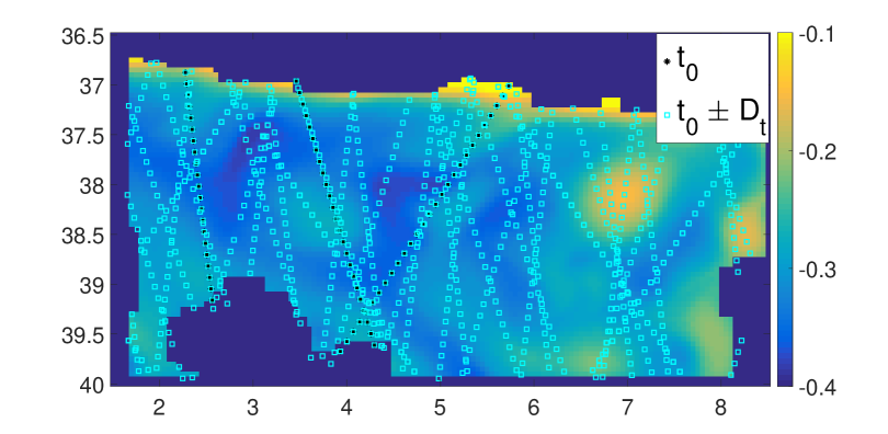
Figure 1 reports an example of the considered sampling patterns. We let the reader refer to Section 3 for the detailed description of the considered application to ocean remote data.
The reconstruction of high-resolution image $Y(t)$ given low-resolution image $Y_{LR}(t)$ is stated according to the following convolution-based model:

$$Y(t)=Y_{LR}(t)+H_{Y}*Y_{LR}(t)+H_{X}*X(t)+N(t)$$ (1)

where $N$ is a space-time noise process. $H_{Y}$ (resp. $H_{X}$) is the two-dimensional impulse response of the $Y_{LR}$ (resp. $X$) component of the proposed convolutional model. $H_{Y}$ and $H_{X}$ are characterized by $(2W_{p}+1)\times(2W_{p}+1)$ discrete representations onto the considered high-resolution grid. Importantly, $H_{Y}$ and $H_{X}$ are space-and-time-varying operators and capture the space-time variabilities of $(Y,Y_{LR})$ and $(Y,X)$ relationships. This model can be regarded as a patch-based super-resolution approach where high-resolution image $Y$ at a given location is computed as a linear combination of $(2*W_{p}+1)\times(2*W_{p}+1)$ patches of images $X$ and $Y_{LR}$ centered at the same location. Parametrization $H_{X}=0$ clearly relates to regression-based super-resolution models [7, 6].

2.2 Unconstrained model calibration

The calibration of model (1) amounts to the estimation of the $(2W_{p}+1)\times(2W_{p}+1)$ matrix representations of operators $H_{Y}$ and $H_{X}$ at any space-time location. The availability of the irregularly-sampled dataset $\{\tilde{t}(k),\tilde{s}(k),\tilde{Y}(k)\}_{k}$ provides the means for this locally-adapted calibration. It may be noted that, in classical image super-resolution issue, such models are trained offline or involve nearest-neighbor techniques using a training dataset of joint low-resolution and high-resolution image patches [7, 6]. Here, we proceed as follows. For a given space-time location $(t_{0},s_{0})$, we regard all data such that $\tilde{t}(k)\in[t_{0}-D_{t},t_{0}+D_{t}]$ and $\|\tilde{s}(k)-s_{0}\|\leq D_{s}$ as observations for model (1) at location $(t_{0},s_{0})$. Parameters $D_{t}$ and $D_{s}$ state respectively the spatio-temporal extent of the considered neighborhood around location $(t_{0},s_{0})$. Given the irregular sampling of the high-resolution dataset, no guarantees exist that sampling locations $\tilde{s}(k)$ will lie within the considered $X$/$Y_{LR}$ grid, and thus $(2W_{p}+1)\times(2W_{p}+1)$ high-resolution $X$ patches and low-resolution $Y_{LR}$ patches need to be interpolated around spatio-temporal locations $(\tilde{s}(k),\tilde{t}(k))$. Local impulse responses $H_{X}$ and $H_{Y}$ are then fitted by minimizing the mean square reconstruction error $\mathcal{E}\left(H_{X},H_{Y}\right)$ for the high-resolution detail $dY=Y-Y_{LR}$ at irregularly-sampled dataset positions $(\tilde{s}(k),\tilde{t}(k))$:

$$\mathcal{E}\left(H_{X},H_{Y}\right)=\sum\limits_{k}\left|\left|d\tilde{Y}\left(k\right)-\widehat{d\tilde{Y}}\left(k\right)\right|\right|^{2}$$ (2)

$$\mbox{where}\quad\widehat{d\tilde{Y}}(k)= H_{Y}*Y_{LR}\left(\tilde{t}\left(k\right),\tilde{s}\left(k\right)\right)+$$ (3)

$$H_{X}*X\left(\tilde{t}\left(k\right),\tilde{s}\left(k\right)\right)$$

Assuming the number of observations is high-enough, minimization (2) resorts to a least-square estimation of operators $H_{Y}$ and $H_{X}$.

2.3 Dictionary-based decompositions

A critical aspect of the above least-square minimization is the number of available training data points and the underlying balance between locally-adapted and robust parametrizations. With a view to improving estimation robustness as well model interpretability, we explore dictionary-based decomposition approaches. They resort to the following decomposition of operators $H_{X}$ and $H_{Y}$:

$$H_{\{X,Y\}}=\sum_{k=1}^{K}\alpha_{k}D_{k}^{\{X,Y\}}$$ (4)

where $D_{k}^{Y}$ (resp. $D_{k}^{X}$) is the k^th component of the dictionary of operators for operator $H_{Y}$ (resp. $H_{X}$) and $\alpha_{k}$ is the k^th scalar coefficient that states the decomposition of operator $H_{Y}$ (resp. $H_{X}$) onto dictionary element $D_{k}^{Y}$ (resp. $D_{k}^{X}$). It should be noted that a joint dictionary-based representation is considered in our study, so that decomposition coefficients $\alpha_{k}$ are shared by the two convolutional operators $H_{Y}$ and $H_{X}$.
Following classical dictionary-based settings [11], we explore their applications to convolution operators. We investigate three different types of constraints for dictionary elements $\{D_{k}^{Y}\}$ and decomposition coefficients $\{\alpha_{k}\}$: namely orthogonality, sparsity and non-negativity constraints. The calibration of these dictionary-based settings first involve the estimation of dictionary elements $\{D_{k}^{Y}\}$ using training data. We here assume we are provided with a representative dataset of unconstrained estimates of operators $H_{Y}$ and $H_{X}$ from (2), denoted by $\{H^{n}_{Y},H^{n}_{X}\}_{n}$. More precisely, the considered dictionary-based decompositions are as follows:

• Orthogonality constraint: under this constraint, dictionary elements $\{D_{k}^{Y}\}$ form an orthonormal basis with no other constraints onto coefficients $\{\alpha_{k}\}$. This decomposition relates to the application of principal component analysis (PCA) [12] to dataset $\{H^{n}_{Y},H^{n}_{X}\}_{n}$. Given the trained dictionary, the estimation of decomposition coefficients $\{\alpha_{k}\}$ comes to the projection of the unconstrained operator estimates onto dictionary elements $\{D_{k}^{Y}\}$.

• Sparsity constraint: the sparse dictionary-based decomposition [13] resorts to complementing MSE criterion (2) with the $L_{1}$ norm of coefficients $\{\alpha_{k}\}$. We apply a KSVD scheme to dataset $\{H^{n}_{Y},H^{n}_{X}\}_{n}$ to train dictionary elements $\{D_{k}^{Y}\}$. Given the trained dictionary, we proceed similarly to kSVD and use orthogonal matching pursuit [14] for the sparse estimation of decomposition coefficients $\{\alpha_{k}\}$ for any new unconstrained operator estimate.

• Non-negativity constraint: the non-negative dictionary-based decomposition constrains coefficients $\{\alpha_{k}\}$ to be non-negative. Given dataset $\{H^{n}_{Y},H^{n}_{X}\}_{n}$, the training of dictionary elements $\{D_{k}^{Y}\}$ resorts to the minimization of reconstruction error (2) under non-negativity constraints for the decomposition coefficients. We exploit an iterative proximal operator-based algorithm [15]. Given the trained dictionary, the estimation of decomposition coefficients $\{\alpha_{k}\}$ comes to a least-square estimation under non-negativity constraints.

2.4 Locally-adapted dictionary-based convolutional models

Fig. 1: Illustration of the irregular sampling of high-resolution observations associated with ocean remote sensing data: sea surface height image with the sampled along-track positions by satellite altimeters (cyan squares) in a $\pm 10$-day time window around April $20^{th}$, 2012.

The application of the proposed dictionary-based decompositions to the super-resolution of irregularly-sampled high-resolution images involves the following main steps. For a given dictionary-based decomposition, we first train the associated dictionaries $\{D_{k}^{X},D_{k}^{Y}\}$. Considering the entire image time series, we proceed to the unconstrained estimation of operators $H_{X}$ and $H_{Y}$ from (2) for a variety of spatio-temporal neighborhoods with given parameters $D_{s}^{Tr}$ and $D_{t}^{Tr}$. Parameters $D_{s}^{Tr}$ and $D_{t}^{Tr}$ are set such that the number of high-resolution observations is high enough to solve for least-square criterion (2). We typically sample around 1500 neighborhoods to build a representative dataset of operators $H_{X}$ and $H_{Y}$.
Given the trained dictionaries, we proceed to the super-resolution of an image at a given date $t^{*}$ as follows. For any given spatial location $s^{*}$, we first estimate the associated decomposition coefficients $\{\alpha_{k}\}$ from the subset of high-resolution observations in a spatio-temporal neighborhood of space-time location $(t^{*},s^{*})$ with parameters $D_{s}^{SR}$ and $D_{t}^{SR}$. The later parameters typically define smaller spatio-temporal neighborhoods than training neighborhoods with parameters $D_{s}^{Tr}$ and $D_{t}^{Tr}$. As such, estimated coefficients $\{\alpha_{k}\}$ come to the projection of more local convolutional operators onto the subspace spanned by the estimated dictionaries, thus yielding a more locally-adapted model (1). This calibrated model is then applied to the reconstruction of image $Y$ in a neighborhood of location $(t^{*},s^{*})$. To reduce the computational time, we perform this calibration of locally-adapted models for a regular subsampling of the image grid, typically $D_{s}^{SR}/2$, and use a spatial averaging of overlapping local reconstructions to obtain a single high-resolution reconstruction of image $Y$.

3 Experiments

Fig. 2: Probability distribution for the relative root mean square reconstruction error (RMSE) for daily high-resolution SSH images $\{Y(t)\}_{t}$, for a global convolutional model and for locally-adapted decompositions of a global convolutional model using principal component analysis (PCA) [12], KSVD [13] and non-negative decomposition (NN) and considering $K=10$ classes. The probability distribution of the RMSE for daily low-resolution SSH images $\{Y_{LR}(t)\}_{t}$ is given as reference (noted as $SSH_{LR}$).

	$K=2$	$K=5$	$K=10$
PCA	0.1807	0.1734	0.1680
KSVD	0.2228	0.2228	0.2228
NN	0.1807	0.1734	0.1666
Global model			0.1755
$SSH_{LR}$			0.2228

Table 1: Relative root mean square reconstruction error (RMSE) for daily high-resolution SSH images $\{Y(t)\}_{t}$, for a global convolutional model and for locally-adapted decompositions of a global convolutional model using principal component analysis (PCA) [12], KSVD [13] and non-negative decomposition (NN), considering $K=2$, $K=5$ and $K=10$ classes. The RMSE value for daily low-resolution SSH images $\{Y_{LR}(t)\}_{t}$ is given as reference (noted as $SSH_{LR}$). Best results for each number of classes $K$ considered are presented in bold. Results that outperform a global convolutional model are underlined.

Fig. 3: High-resolution SSH image $Y$ reconstruction, April 20^th, 2012: first row, from left to right, real high-resolution SSH image $Y$, low-resolution SSH image $Y_{LR}$ (noted as $SSH_{LR}$), reconstruction of high-resolution SSH image $Y$ using global convolutional model (1); second row, reconstruction of high-resolution SSH image $Y$ using a 10-class locally-adapted decomposition (4) of global convolutional model (1) using, from left to right, principal component analysis (PCA) [12], KSVD [13] and non-negative decomposition (NN).

As case study, we consider an application to ocean remote sensing data, more particularly to the reconstruction of sea-surface height (SSH) image time series from along-track altimeter data. Satellite altimeters are narrow-swath sensors such that high-resolution altimeter data is only acquired along the satellite track path [16], resulting in an particularly scarce and irregular sampling of the ocean surface as illustrated in Fig.1. Interestingly, numerous studies have pointed out the potential contribution of high-resolution sea surface temperature (SST) images to the reconstruction of SSH images, as they share common geometrical patterns associated with the underlying upper ocean dynamics [17, 18]. In addition, optimally-interpolated products [16] provide a low-resolution reconstruction of the SSH image. Overall, the reconstruction of high-resolution SSH image time series resorts to a super-resolution issue from irregularly-sampled high-resolution information as stated in Section 2. It may be stressed that this case study involves a scaling factor of about 10 between the low-resolution and high-resolution data, which makes it particularly challenging compared with classical image super-resolution issues.
In our experiments, we exploit a ground-truthed dataset using an observing system simulation experiment for a case study region in the Western Mediterranean Sea ($36.5\degree N$ to $40\degree N$, $1.5\degree E$ to $8.5\degree E$). A high-resolution numerical simulation of the WMOP model [19] is used to generate daily high-resolution SSH images from 2009 to 2013 for a $1/20\degree$ grid. The along-track dataset is simulated by sampling the SSH images at real along-track positions issued from from multiple altimetry missions in 2014 and 2015 (see Figure 1). Given the simulated along-track dataset, optimally-interpolated SSH fields [16], referred to as low-resolution SSH images $Y_{LR}$, are computed for a $1/8\degree$ grid resolution. The calibration of the proposed convolutional operators is performed by considering $W_{p}=1$, which corresponds to $3\times 3$ convolutional masks. We use the following parameter setting for spatio-temporal neighborhoods: $t_{0}\pm D_{t}$-day time windows with $D_{t}=10$, and $D_{s}\times D_{s}$ spatial neighborhoods with $D_{s}^{Tr}=7\degree$ for the training step and $D_{s}=2\degree$ for the locally-adapted calibration steps.
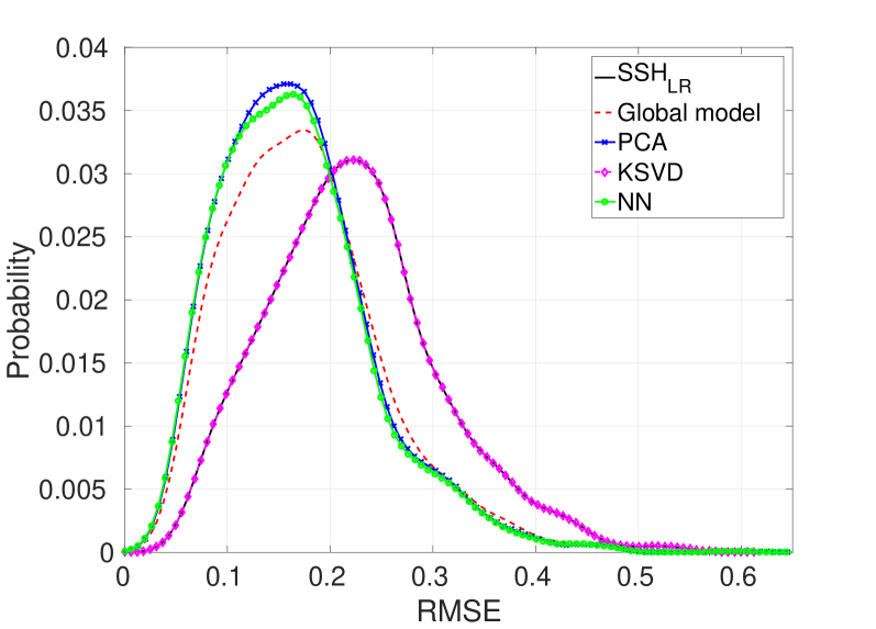
In Table 1, we report the average root mean square reconstruction error (RMSE) for daily high-resolution SSH images $\{Y(t)\}_{t}$, for a global convolutional model and for locally-adapted convolutional models, using principal component analysis (PCA) [12], KSVD [13] and non-negative dictionary-based decomposition (NN) and considering $K=2$, $K=5$ and $K=10$ elements in the dictionaries. The reconstruction RMSE for daily low-resolution SSH images $\{Y_{LR}(t)\}_{t}$ (noted as $SSH_{LR}$) is given as reference.
From Table 1, locally-adapted convolutional models clearly outperform global models for $K\geq 5$ (with the exception of the KSVD-based decomposition), which can be explained by the improved local adaptation to local spatio-temporal variabilities through locally-adapted decomposition coefficients. In this respect, the non-negative decomposition outperforms alternative approaches, with a maximum relative gain (with respect to optimally-interpolated low-resolution SSH images $\{Y_{LR}(t)\}_{t}$, at $K=10$) of 25.22% for NN, 24.60% for PCA and 21.23% for a global convolutional model.
These results are further illustrated by the reconstruction of high-resolution SSH image $Y$ for sample date April 20^th, 2012 presented in Figure 3 and by the probability distributions of daily reconstruction root mean square error for high-resolution SSH images $\{Y(t)\}_{t}$, computed for the global convolutional model and for each one of the considered locally-adapted models with $K=10$, presented in Figure 2. Visually, the proposed super-resolution models clearly improve the reconstruction of finer-scale details compared to the low-resolution image. The model using non-negativity constraints seems to involve slightly sharper gradients compared with the unconstrained model. The PCA-based model appears visually less relevant, while the KSVD-based model seems unable to exploit the high-resolution information sources to enhance the low-resolution altimetry field.

4 Conclusion

In this paper, we addressed the multimodal super-resolution of irregularly-sampled high-resolution images. This issue arises in a number of remote sensing applications, where several sensors associated with different regular and irregular sampling patterns may contribute to the reconstruction of a given high-resolution image. As a case study, we considered an application to the reconstruction of high-resolution sea surface height (SSH) images. From a methodological point of view, we complement previous convolution-based super-resolution models [7, 8] with the evaluation of different dictionary-based decompositions and the use of a complementary high-resolution image source. Dictionary-based decompositions are regarded as a means to better account for spatio-temporal variabilities through more locally-adapted model calibrations. Our numerical experiments support the selection of non-negativity constraints to achieve a better local adaptation. They demonstrate the relevance of the proposed approach to achieve a better reconstruction of higher-resolution details, compared with the optimally-interpolated fields.
Future work includes non-local extensions of the proposed model to combine spatio-temporal and similarity-based neighborhoods as considered in regression-based super-resolution models [7, 8]. Non-linear dictionary-based decomposition seems particularly appealing to combine non-linear mapping, for instance CNN-based models [20], and locally-adapted models. As far as ocean remote sensing applications are considered, applying the proposed models to different sampling patterns, for instance along-track narrow-swath satellite data vs. wide-swath satellite data, appears to be of interest, the later possibly enabling the modeling of higher-order geometrical details.

References

- [1] W. C. Siu and K. W. Hung, “Review of image interpolation and super-resolution,” in Proceedings of The 2012 Asia Pacific Signal and Information Processing Association Annual Summit and Conference, Dec 2012, pp. 1–10.
- [2] D. Glasner, S. Bagon, and M. Irani, “Super-resolution from a single image,” in 2009 IEEE 12th International Conference on Computer Vision, Sept 2009, pp. 349–356.
- [3] D. Yang, Z. Li, Y. Xia, and Z. Chen, “Remote sensing image super-resolution: Challenges and approaches,” in 2015 IEEE International Conference on Digital Signal Processing (DSP), July 2015, pp. 196–200.
- [4] R. Fablet and F. Rousseau, “Joint interpolation of multisensor sea surface temperature fields using nonlocal and statistical priors,” IEEE Journal of Selected Topics in Applied Earth Observations and Remote Sensing, vol. 9, no. 6, pp. 2665–2675, June 2016.
- [5] M. E. Gheche, J. F. Aujol, Y. Berthoumieu, C. A. Deledalle, and R. Fablet, “Texture synthesis guided by a low-resolution image,” in 2016 IEEE 12th Image, Video, and Multidimensional Signal Processing Workshop (IVMSP), July 2016, pp. 1–5.
- [6] R. Timofte, V. De Smet, and L. Van Gool, “Anchored neighborhood regression for fast example-based super-resolution,” in The IEEE International Conference on Computer Vision (ICCV), December 2013.
- [7] R. Timofte, V. De Smet, and L. Van Gool, “A+: Adjusted anchored neighborhood regression for fast super-resolution,” in Asian Conference on Computer Vision. Springer, 2014, pp. 111–126.
- [8] E. Agustsson, Timofte R., and L. Van Gool, “Regressor Basis Learning for Anchored Super-Resolution,” in IEEE International Conference on Pattern Recognition (ICPR), Cancun, Mexico, Dec. 2016.
- [9] M. Bevilacqua, A. Roumy, C. Guillemot, and M. L. Alberi Morel, “Low-complexity single-image super-resolution based on nonnegative neighbor embedding,” .
- [10] J. Yang, J. Wright, T.S. Huang, and Y. Ma, “Image super-resolution via sparse representation,” IEEE Transactions on Image Processing, vol. 19, no. 11, pp. 2861–2873, Nov 2010.
- [11] B. A. Olshausen and D. J. Field, “Sparse coding with an overcomplete basis set: A strategy employed by v1?,” Vision Research, vol. 37, no. 23, pp. 3311 – 3325, 1997.
- [12] K. Pearson, “On lines and planes of closest fit to systems of points in space,” Philosophical Magazine Series 6, vol. 2, no. 11, pp. 559–572, 1901.
- [13] M. Aharon, M. Elad, and A. Bruckstein, “K-SVD: An algorithm for designing overcomplete dictionaries for sparse representation,” IEEE Transactions on Signal Processing, vol. 54, no. 11, pp. 4311–4322, Nov 2006.
- [14] Y. C. Pati, R. Rezaiifar, and P. S. Krishnaprasad, “Orthogonal matching pursuit: recursive function approximation with applications to wavelet decomposition,” in Proceedings of 27th Asilomar Conference on Signals, Systems and Computers, Nov 1993, pp. 40–44 vol.1.
- [15] P. L. Combettes and J.C. Pesquet, “Proximal Splitting Methods in Signal Processing,” in Fixed-Point Algorithms for Inverse Problems in Science and Engineering, H.H Bauschke, R.S. Burachik, P.L. Combettes, V. Elser, D.R. Luke, and H. Wolkowicz (Eds.), Eds., pp. 185–212. Springer, 2011.
- [16] M. I. Pujol and G. Larnicol, “Mediterranean sea eddy kinetic energy variability from 11 years of altimetric data,” Journal of Marine Systems, vol. 58, no. 3–4, pp. 121–142, Dec. 2005.
- [17] G. Lapeyre and P. Klein, “Dynamics of the upper oceanic layers in terms of surface quasigeostrophy theory,” 2006.
- [18] P. Klein, B.L. Hua, G. Lapeyre, et al., “Upper ocean turbulence from high-resolution 3d simulations,” 2008.
- [19] M. Juza, B. Mourre, L. Renault, S. Gómara, K. Sebastián, S. Lora, J. P. Beltran, B. Frontera, B. Garau, C. Troupin, M. Torner, E. Heslop, B. Casas, R. Escudier, G. Vizoso, and J. Tintoré, “SOCIB operational ocean forecasting system and multi-platform validation in the Western Mediterranean Sea,” Journal of Operational Oceanography, vol. 9, no. sup1, pp. s155–s166, Feb. 2016.
- [20] C. Dong, C. C. Loy, K. He, and X. Tang, “Image super-resolution using deep convolutional networks,” IEEE Transactions on Pattern Analysis and Machine Intelligence, vol. 38, no. 2, pp. 295–307, Feb 2016.