High-Fidelity Preservation of Quantum Information During Trapped-Ion Transport

Abstract

A promising scheme for building scalable quantum simulators and computers is the synthesis of a scalable system using interconnected subsystems. A prerequisite for this approach is the ability to faithfully transfer quantum information between subsystems. With trapped atomic ions, this can be realized by transporting ions with quantum information encoded into their internal states. Here, we measure with high precision the fidelity of quantum information encoded into hyperfine states of a ¹⁷¹Yb⁺ ion during ion transport in a microstructured Paul trap. Ramsey spectroscopy of the ion’s internal state is interleaved with up to $4000$ transport operations over a distance of $280\text{\,}\mathrm{\SIUnitSymbolMicro}\mathrm{m}$ each taking $12.8\text{\,}\mathrm{\SIUnitSymbolMicro}\mathrm{s}$. We obtain a state fidelity of $99.9994\left({}^{+6}_{-7}\right)$% per ion transport.

Ion traps have been a workhorse in demonstrating many proof-of-principle experiments in quantum information processing using small ion samples Blatt and Wineland (2008). A major challenge to transform this ansatz into a powerful quantum computing machine that can handle problems beyond the capabilities of classical super computers remains its scalability Kielpinski et al. (2002); Svore et al. (2006); Monroe et al. (2014); Lekitsch et al. (2017). Error correction schemes allow us to fight the ever sooner death of fragile quantum information stored in larger and larger quantum systems, but their economic implementation requires computational building blocks to be executed with sufficient fidelity Shor (1995); Steane (1996). Essential computational steps have been demonstrated with fidelities beyond a threshold of $99.99\%$ that is often considered as allowing for economic error correction Knill (2010), and, thus for fault-tolerant scalable quantum information processing (QIP). These building blocks include single qubit rotation Brown et al. (2011); Ballance et al. (2016), individual addressing of interacting ions  Piltz et al. (2014), and internal state detection Burrell et al. (2010). In addition, high fidelity two-qubit quantum gates Benhelm et al. (2008); Ballance et al. (2016); Harty et al. (2016); Gaebler et al. (2016); Weidt et al. (2016) and coherent three-qubit conditional quantum gates Monz et al. (2009); Piltz et al. (2016) have been implemented.

Straightforward scaling up to an arbitrary size of a single ion trap quantum register, at present, appears unlikely to be successful because the growing size of a single register usually introduces additional constraints imposed by the confining potential and by the Coulomb interaction of ion strings Johanning (2016). Even though, for instance, transverse modes and anharmonic trapping Lin et al. (2009) may be employed for conditional quantum logic, a general claim might be that, at some point it is useful to divide a single ion register into subsystems and to exchange quantum information between these subsystems Kielpinski et al. (2002); Svore et al. (2006); Monroe et al. (2014); Lekitsch et al. (2017). One might do that by transferring quantum information from ions to photons (and vice versa) and by then exchanging photons between subsystems Monroe et al. (2014); Hucul et al. (2015).

Alternatively, when exchanging quantum information between spatially separated individual registers within an ion trap-based quantum information processor, the transport of ions carrying this information is an attractive approach Kielpinski et al. (2002); Svore et al. (2006); Lekitsch et al. (2017). Methods to transport ions in segmented Paul traps have been developed and demonstrated Rowe et al. (2002); Hensinger et al. (2006); Blakestad et al. (2009); Singer et al. (2010), and optimized with respect to the preservation of the motional state during transport Bowler et al. (2012); Walther et al. (2012).

It is equally important to avoid errors of the quantum information encoded into internal states of ions during transport. Schemes relying on physical transport of ions require shuttling of ions between regions where the actual conditional gates take place (or between memory zones). Transport and single qubit manipulation can also be combined and executed at the same time de Clercq et al. (2016).

Quantum error correction relies on the distribution of a logical qubit’s information onto multiple qubits. Encoding and correction of this information consists, in general, of a number of single qubit rotations, entangling gates, measurements, and typically either shuttling or spectroscopic decoupling of ions. To have the entire error correction sequence be beneficial, the constraints on the individual operations are obviously more stringent. For all correction schemes involving ion transport, the number of transport operations are bigger compared to or much larger than one Kielpinski et al. (2002); Chiaverini et al. (2005); Svore et al. (2006); Lekitsch et al. (2017), so the infidelity must, at least, be an order of magnitude smaller than acceptable for the entire sequence.

Therefore, in addition to high fidelity local gates, high fidelity transport is required to not cross a desired error threshold when carrying out single- and multiqubit quantum gates.

Several experiments have characterized the internal state fidelity ${\mathcal{F}}=\expectationvalue{\rho}{\psi}$ upon transport by measuring the loss of coherence of a prepared superposition state $\ket{\psi}$ which dephases into a mixed state $\rho$ during a Ramsey-type measurement. However, the precision reached in these experiments was not yet sufficient to conclude that transport takes place in the fault-tolerant regime required for scaling Rowe et al. (2002); Blakestad et al. (2009); Bowler et al. (2012); Walther et al. (2012). Here, we demonstrate high fidelity transport of trapped ions over a distance of $280\text{\,}\mathrm{\SIUnitSymbolMicro}\mathrm{m}$ with quantum information encoded into internal hyperfine states with a relative error of the qubit states per transport below $10^{-5}$ which is compatible with fault-tolerant and, thus, scalable quantum computation.

The determination of ${\mathcal{F}}$ is limited by the uncertainty of the extracted Ramsey-fringe contrast and the relative error is of the same order as the relative uncertainty of the contrast. In the experiments reported below, we determine the contrast of a Ramsey-type measurement typically with a relative error of $\leq 1\text{\times}{10}^{-2}$. Therefore, the straightforward extraction of fringe contrast from experimental data is not sufficient for precise determination of the error taking place during transport. To be able to precisely measure the loss of fidelity, we increase the number of transport operations $M$. To limit systematic errors due to a possible spatial variation of the qubit coherence time in the trap, we design the experiment such that the ions’ average position is independent of $M$ for $M>0$ and compare the contrast after $M=4000$ with the contrast obtained after $M=2$ transport operations.

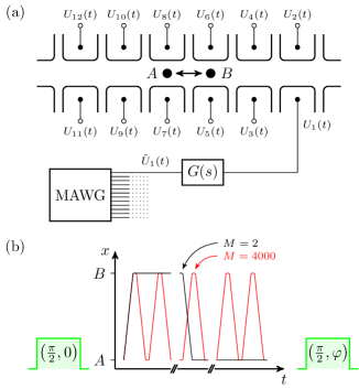
Figure 1: Schematic of the experiment. (a) The voltages $\tilde{U}(t)$ at the multichannel arbitrary waveform generator (MAWG) take the filter characteristic $G(s)$ of the electronics into account to produce suitable voltages $U(t)$ that transports the ion along the x axis $M$ times between positions $A$ and $B$. (b) The timing of the transport operations is such that the ion is located equally long at $A$ and $B$. The ion transfer is sandwiched by two $\pi/2$-pulses.

The ion trap is operated with singly charged ¹⁷²Yb and ¹⁷¹Yb ions. ¹⁷²Yb⁺ ions possessing no hyperfine structure are employed to determine the efficiency of physical ion transport, while for the analysis of the transport induced decoherence, a hyperfine qubit in ¹⁷¹Yb⁺ is used. As a qubit, we choose the first-order magnetic field insensitive hyperfine qubit composed of the states $\ket{0}\equiv\ket{S_{\nicefrac{{1}}{{2}}},F=0}$ and $\ket{1}\equiv\ket{S_{\nicefrac{{1}}{{2}}},F=1,m_{F}=0}$. The second order magnetic field sensitivity of the qubit resonance frequency at $B=$640\text{\,}\mathrm{\SIUnitSymbolMicro T}\text{/}$$ is $d\nu/dB=$39.7\text{\,}\mathrm{MHz}\text{/}\mathrm{T}$$. A detailed description of the laser and microwave setup can be found in Vitanov et al. (2015).

The experiment is carried out in a 3D-Paul trap Kaufmann et al. (2012); Schulz et al. (2006, 2008); Baig et al. (2013) divided into 33 segments, each consisting of two dc electrodes, and two global rf electrodes. In the experiments reported here, ions were transported by moving the minimum of the trapping potential from the center of one segment $A$ to the center of the next segment $B$ over a distance of $280\text{\,}\mathrm{\SIUnitSymbolMicro}\mathrm{m}$ (see Fig. 1). The required potentials were generated by applying twelve voltage ramps to dc electrodes of six trap segments of the trap. One additional voltage ramp was applied to a correction electrode to allow for minimization of micromotion perpendicular to the dc electrodes’ plane.

Methods to transport ions in segmented Paul traps have been investigated elaborately in a number of publications Rowe et al. (2002); Hensinger et al. (2006); Blakestad et al. (2009, 2011); Walther et al. (2012). We use the approach worked out in Ref. Torrontegui et al. (2011) to calculate an optimized trajectory ${\mathbf{r}}(t)$ that minimizes ion heating during transport, an implementation of the boundary element method to simulate the potentials generated by our trap geometry Singer et al. (2010), and the formalism described in Ref. Blakestad et al. (2011) to calculate suitable transport voltages. To reduce limitations of the potential dynamics imposed by low pass filters of our dc electrodes, we extend this formalism by a method to constructively take into account the filter characteristics: Instead of trying to compensate the filter behavior after the transport voltage ramps $U(t)$ have been determined, we calculate the accessible voltage range for every point ${\mathbf{r}}_{i}={\mathbf{r}}(t_{i})$ during transport based on the voltage history $U(t_{k<i})$ and limit the potential optimization algorithm to this interval. Using this approach, we are able to realize single transport times of $12.8\text{\,}\mathrm{\SIUnitSymbolMicro s}\text{/}$ on the order of the inverse filter cut off frequency ($15.8\text{\,}\mathrm{\SIUnitSymbolMicro s}\text{/}$). See Supplemental Material (Section I on page I) for details.

In the experiment presented in this Letter, we performed $22\text{\times}{10}^{6}$ transport operations without losing an ion. The success of a single transport operation $A\rightarrow B$ or $B\rightarrow A$ is proven by imaging the ion fluorescence for a few milliseconds once the ion is at rest after transport. Because up to $2000$ consecutive transport operations $A\rightarrow B\rightarrow A$ are investigated, the success of the overall transport (i.e., during $M$ shuttling events) needs to be shown as well. Imaging the ion for several milliseconds at one position after every second transport operation would add seconds to every single repetition of the experiment, and, more importantly, change the transport dynamics by doppler-cooling of the ions. So to diagnose the success rate of consecutive transfers, we implemented an experiment to track the ion during $M$ shuttling operations. During the transport operation the electron multiplying charged-coupled device camera takes one single image with an exposure time equal to the overall transport duration. Synchronized to the ion transport, we flash the detection laser at position $A$ ($B$) for $2\text{\,}\mathrm{\SIUnitSymbolMicro}\mathrm{s}$ each time the ion should be at position $B$ ($A$). The absence of the ion is signified by not detecting scattered resonance fluorescence. This experiment is not exactly tracking the ion, but it proves that it is not at a position where it should not be. We also perform measurements that flash the ion at position $A$ ($B$) when it is expected to be there, but the statistics of these measurements are a factor $15$ inferior compared to the more sensitive detection of an absent ion. This experiment is carried out using ¹⁷²Yb⁺, to profit from higher fluorescence rates. The analysis yields that $8\left({}^{+12}_{-8}\right)$ out of $4000$ transport operations are failing. This number corresponds to a transport fidelity (the probability of transporting the ion as intended) of $99.8\text{\,}\mathrm{\char 37\relax}\text{/}$. Combined with the ions presence after $22\text{\times}{10}^{6}$ transport operations, we interpret the obtained transport fidelity as a lower bound. See Supplemental Material (Section II on page II) for a detailed analysis of the transport fidelity.

The central goal of the Letter presented here is to determine the effect of ion transport operations on the qubit’s internal state coherence. The internal state coherence is determined by performing a Ramsey-type experiment, where transport operations are executed during the free precession time: We initialize the qubit of a Doppler-cooled ion at position $A$ in the $\ket{0}$ state. Using a microwave $\pi/2$ pulse, we prepare the superposition state $\ket{\psi}=1/\sqrt{2}(\ket{0}-i\ket{1})$. Next, the ion is transported $M$ times between the positions $A$ and $B$. We add waiting times at the positions $A$ and $B$ such that the total precession time $t_{p}=$69.44\text{\,}\mathrm{ms}\text{/}$$ is independent of $M$.

The waiting time is equally distributed between both positions. After a second $\pi/2$ pulse with a phase $\varphi$ relative to the first pulse, the qubit state is read out.

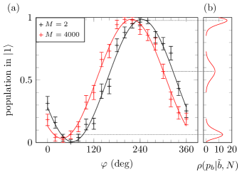
Figure 2: (a) Ramsey fringes for $1$ (black) and $4000$ (red) ion transport operations. The relative phase $\varphi$ between the two $\pi/2$-pulses is varied while the time between the pulses is kept constant. The decay of the amplitude due to the additional transport operations is hardly noticeable. (b) Three examples for the probability distributions that were used for the likelihood analysis of the data. The probability density $\rho(p_{b}|\tilde{b},N)$ for $\tilde{b}$ bright events out of $N$ trials is shown on the horizontal axis as a function of the probability $p_{b}$ for a projection into the state $\ket{1}$ on the vertical axis.

We sample the Ramsey interference fringe for $M=2$ and $M=4000$ transport operations at $19$ phase values $\varphi$. The Ramsey measurement for every setting is repeated $100$ times (see Fig. 2).

We monitor fluorescence during Doppler-cooling and use a low fluorescence count (dark or absent ion) as a veto for the last and next Ramsey measurement (about $10\text{\,}\mathrm{\char 37\relax}\text{/}$ of the data). Besides electronic readout noise and background counts, the detection scheme is limited by off resonant excitation of the transitions $\ket{{S}_{\nicefrac{{1}}{{2}}},F=0}-\ket{{P}_{\nicefrac{{1}}{{2}}},F=1}$ and $\ket{{S}_{\nicefrac{{1}}{{2}}},F=1}-\ket{{P}_{\nicefrac{{1}}{{2}}},F=1}$ and following decay into $\ket{{S}_{\nicefrac{{1}}{{2}}},F=1}$ resp. $\ket{{S}_{\nicefrac{{1}}{{2}}},F=0}$. The former process results in the observation of fluorescence from a qubit originally in the $\ket{0}$ (dark) state, the latter one reduces the fluorescence of the $\ket{1}$ (bright) state. The same effect can be induced by spontaneous decay of the $\ket{{P}_{\nicefrac{{1}}{{2}}},F=0}$ state to the $\ket{{D}_{\nicefrac{{3}}{{2}}},F=1}$ state. By using two separate discrimination thresholds for dark and bright states in the data analysis, we can reduce the probability of wrongly identified states at the cost of reduced statistics Vitanov et al. (2015); Wölk et al. (2015).

For threshold selection, we add calibration runs to the experiment in which we omit the $\pi/2$ pulses but prepare the ion in the $\ket{0}$ ($\ket{1}$) state before the transport operations, to obtain detection histograms for pure $\ket{0}$ ($\ket{1}$) states. The $\ket{1}$ state is prepared by using a BB1RWR $\pi$ pulse Cummins et al. (2003) that is robust against Rabi frequency errors. The calibration is done separately for both $M=2$ and $M=4000$ transport operations in order to account for possible variations of the detection statistics due to transport induced ion heating. Using these calibration measurements, we determine threshold values for state discrimination. In addition, the probabilities to correctly identify a bright state as bright $p_{\tilde{b}|b}$ and a dark state as dark $p_{\tilde{d}|d}$ can be extracted. We choose thresholds that yield $p_{\tilde{b}|b}=0.964$ ($0.959$) and $p_{\tilde{d}|d}=0.985$ ($0.978$) for $M=4000$ ($M=2$).

The determination of coherence loss of the qubit state due to the transport operations is done by comparing the amplitudes of the obtained Ramsey fringes for different numbers of transport operations $M$. As we expect the infidelity to be close to zero, we need to employ several statistical methods to get precise results and error estimates. Since the efficiency of state selective detection is below unity, we distinguish between the actual number of projections $b$ and $d$ ($b,d\in\mathbb{N}_{0}$ and $b+d=N$) into states $\ket{1}$ and $\ket{0}$ and the corresponding numbers $\tilde{b}$ and $\tilde{d}$ identified as $\ket{1}$ and $\ket{0}$ during data analysis. To reconstruct the true fractional population of the states $\ket{0}$ and $\ket{1}$ of a qubit state $\ket{\psi}$, we need to infer the numbers $b$ and $d$ from the numbers of identified states $\tilde{b}$ and $\tilde{d}$.

The obtained probability density $\rho(p_{b}|\tilde{b},N)$ of the state population depends on the number of identified bright states, the number of measurements $N$, and the state identification probabilities $p_{\tilde{b}|b}$ and $p_{\tilde{d}|d}$.

The state population varies as a function of the relative phase of the second $\pi/2$ pulse and can be parameterized by

$$p_{b}(\varphi)=B+A\sin(\varphi-\Phi)$$ (1)

with the amplitude $A$, offset $B$, and phase shift $\Phi$. We fit this model by maximizing the log likelihood

$$\log\mathcal{L}_{M}(A,B,\Phi)=\sum_{k=1}^{K}\log\rho(B+A\sin(\varphi_{k}-\Phi)|\tilde{b_{k}},N_{k})$$ (2)

for both numbers of transport operations $M$ using the probability density function $\rho(p_{b}|\tilde{b},N)$ for the $K$ data points $(\tilde{b_{k}},N_{k})$.

The coherence loss of our qubit in a static potential for precession times shorter than $100\text{\,}\mathrm{ms}\text{/}$ is best described by a decay model $A(t)=\frac{1}{2}\exp\left(-\lambda t^{2}\right)$ for the amplitude $A$ of the Ramsey fringe with $\lambda=$4(2)\text{\,}\text{/}{\mathrm{s}}^{2}$$. This corresponds to a expected amplitude of $A(t_{p})=$0.490(5)$$ of a Ramsey measurement without ion transport.

Figure 2(a) shows the Ramsey fringes obtained for $M=2$ and $M=4000$ transport operations. The error bars indicate the $68\text{\,}\mathrm{\char 37\relax}\text{/}$ confidence intervals of single data points. The right part, 2(b), displays the probability distribution $\rho(p_{b}|\tilde{b},N)$ for three exemplary data points. The amplitude of the $M=4000$ curve is slightly reduced by $0.013$ compared to $M=2$, and the phase shift differs by $27\text{\,}\mathrm{\SIUnitSymbolDegree}\text{/}$. We estimate the gradient of the magnetic field in the direction of the ion transport to be $10.6\text{\times}{10}^{-3}\text{\,}\mathrm{T}\mathrm{/}\mathrm{m}$. This gradient results in a $120\text{\,}\mathrm{Hz}\text{/}$ difference between the hyperfine splitting of the qubit at positions $A$ and $B$. From simulations, we expect that the mean positions of the ions for $2$ and $4000$ transfers during the free precession time differ by $0.9\text{\,}\mu\mathrm{m}$, due to non perfect compensation of the dc electrode filters. This would correspond to a phase difference of $10\text{\,}\mathrm{\SIUnitSymbolDegree}\text{/}$. The amplitude reduction observed with the number of transport operations is compatible with zero, in good agreement with our qubit being magnetic field insensitive to the first order. The Supplemental Material (Section III page III) gives a short discussion of different sources for a possible decay The state identification probabilities $p_{\tilde{b}|b}$ and $p_{\tilde{d}|d}$ were treated up to this point as fixed error-free parameters. In reality these values are calculated from a finite set of measurements and therefore bear additional uncertainties. We estimate these uncertainties by analyzing the calibration data obtained for state identification using the bootstrapping resampling method Efron and Tibshirani (1994) and averaging the likelihoods $\mathcal{L}_{M}(A)$ over the results obtained for different choices of $p_{\tilde{b}|b}$ and $p_{\tilde{d}|d}$. See Supplemental Material (Section IV on page IV) for details of the uncertainty estimation

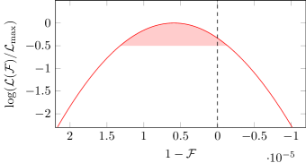
Figure 3: Likelihood of the internal state fidelity ${\mathcal{F}}$ during ion transport. The loss of internal state fidelity due to the transfer of the ion is apparent but the case of no loss of coherence is also compatible within the $68\%$ confidence interval (shaded). The log likelihood is calculated by the numerical convolution of the likelihoods $\mathcal{L}_{M}$.

The likelihood distribution of the internal state fidelity during ion transport (Fig. 3) is calculated by a numerical convolution of the likelihoods of the Ramsey fringe amplitudes $A_{2}$ and $A_{4000}$ according to

$${\mathcal{F}}=\sqrt[4000-2]{\frac{A_{2}}{A_{4000}}}\,.$$ (3)

Here, we report here a fidelity of the internal qubit state per transport operation of

$${\mathcal{F}}=0.999994\left({}^{+6}_{-7}\right)\,.$$ (4)

This result is obtained under the assumption that each individual transport $A\rightarrow B$ and $B\rightarrow A$ out of a total of $M$ attempted transports of an ion is actually successful, that is, the transport fidelity is perfect. Taking a finite probability of transport failure into account, the fidelity would change according to $\overline{{\mathcal{F}}}(M_{f})={\mathcal{F}}^{(\frac{4000-2}{4000-2-M_{f}})}$, for $M_{f}$ failing transports. The likelihood of ${\mathcal{F}}$ is almost gaussian (compare Fig.3), so we expect the error scaling of $\overline{{\mathcal{F}}}$ to follow $\sigma(\overline{{\mathcal{F}}}(M_{f}))=\frac{4000-2}{4000-2-M_{f}}{\mathcal{F}}^{(\frac{M_{f}}{4000-2-M_{f}})}\sigma({\mathcal{F}})$. With the transport fidelity of $99.8\text{\,}\mathrm{\char 37\relax}\text{/}$ determined above, a $5\sigma$ deviation would result in $M_{f}=68$ failed transports. This would reduce the internal state fidelity during ion transport by $1\text{\times}{10}^{-7}$, which is about an order of magnitude smaller than the statistical uncertainty of ${\mathcal{F}}$. A systematic error due to imperfect preparation of the $\ket{0}$ and $\ket{1}$ states also does not change the statistical significance of ${\mathcal{F}}$. See Supplemental Material (Section V page V) for details of the error estimation.

In this work, we use the magnetic insensitive hyperfine qubit. Some schemes for QIP with trapped ions using radio-frequency and microwave radiation Mintert and Wunderlich (2001) utilize magnetic field dependent states, for example, the qubit composed of $\ket{0}$ and $\ket{S_{\nicefrac{{1}}{{2}}},F=1,m_{F}=\pm 1}$. As the magnetic field sensitive qubit can be recoded into the insensitive qubit and back Piltz et al. (2016) the results of this Letter are also immediately relevant for these QIP schemes.

In summary, we demonstrate by precise measurements and careful data analysis that the physical transport of quantum information encoded in a hyperfine qubit can be carried out with a fidelity better than $1-10^{-5}$. This is an important prerequisite, together with high gate fidelities and low cross-talk, for all schemes for scalable QIP with trapped ions that rely on transport of ions.

We acknowledge funding from the European Community’s Seventh Framework Programme under Grant Agreement No. 270843 (iQIT), from EMRP (the EMRP is jointly funded by the EMRP participating countries within EURAMET and the European Union).

Supplemental Material I Transport potentials

The statistical error of the outcome of our experiment is limited both by the number of transport operations $M$ and the number of repetitions $N$. As the transport operations are carried out during the free precession time of a Ramsey experiment with limited coherence time, $M$ is directly limited by the transfer time. $N$ is indirectly limited by the overall stability of the experiment apparatus including microwave and laser power stabilities. In order to improve the statistics we implement fast ion transport that includes micromotion minimization and takes electronic filtering into account.

We use the method presented in Torrontegui et al. (2011) with the parameters axial trap frequency $\omega_{x}=2\pi\times$230\text{\,}\mathrm{kHz}\text{/}$$, transfer distance $\Delta x=$280\text{\,}\mathrm{\SIUnitSymbolMicro}\mathrm{m}$$, a temporal discretization $\Delta t=($12.5\text{\,}\mathrm{MHz}\text{/}$)^{-1}=$80\text{\,}\mathrm{n}\mathrm{s}$$ and transport time $T=160\cdot\Delta t=$12.8\text{\,}\mathrm{\SIUnitSymbolMicro}\mathrm{s}$$ to calculate an ion trajectory ${\mathbf{r}}_{i}={\mathbf{r}}(t=i\cdot\Delta t)$ discretized in $L=160$ single steps.

Next a sequence of $L$ potentials is determined with accordingly chosen potential minima and curvatures at the positions ${\mathbf{r}}_{i}$. For this we first create a set of basis potentials $\Phi^{(j)}({\mathbf{r}})$ of the single electrodes $j$ which are calculated for all electrodes being grounded except electrode $j$ set to a potential $U_{0}$ using the boundary element method software package described in Singer et al. (2010). The transport trapping potentials $\Phi$ are then obtained as a voltage weighted sum of the individual basis potentials $\Phi^{(j)}$ and the rf-pseudopotenial $\Phi^{(ps)}$ of the rf electrodes as presented in Blakestad et al. (2011).

For every step $i$ the potentials have to fullfill a couple of boundary conditions. In this experiment the position of the potential minima imposes $3$ requirements ($\partial_{x,y,z}\Phi=0$), the size of the axial trap frequency $\partial_{x}^{2}\Phi={m}\omega_{x}^{2}/q$ and the alignment of the potential axis parallel to the trap’s $x$-axis ($\partial_{xz}^{2}\Phi=0$) $2$ conditions. We also find it convenient to add a sixth condition $\Phi({\mathbf{r}}_{i})=\Phi_{0}$ to define the field at the location ${\mathbf{r}}_{i}$ of the potential minimum. These conditions can be expressed as operators $\mathcal{P}$ acting on the potential $\Phi=U^{(j)}\Phi^{(j)}+\Phi^{(ps)}$ and their corresponding eigenvalues. As we use 12 independent controllable dc electrode potentials the problem is in principle underconstrained.

In practice the limited voltage range and dynamics of any real voltage source narrows down the possible solutions and yields additional constraints. The available minimal and maximal voltages are primary limiting the accessible potential shapes, while the possible dynamics limits the potential changing speed. For the experiment reported here the latter restriction is of primary concern and for simplicity we will not explicitly write down the constraints by maximal voltages in the following formulas.

If the voltage change per discrete time step is limited by $\delta U$, the possible voltage $U_{i}$ for one dc electrode at step $i$ along the trajectory is limited by

$$U_{i}\lessgtr U_{i-1}\pm\delta U\,.$$ (5)

One can use a constrained optimization algorithm to solve the problem and obtain the voltages $U_{i}^{(j)}$. If not all boundary conditions can be fullfilled at the same time in the given voltage limits (5) it can be beneficial to multiply weight factors to the single boundary conditions and prioritize for example a constant trap frequency over the exact position of the potential minimum.

I.1 Modifications for low-pass filter

It is common practice to low-pass the trap’s dc electrodes in order to reduce the electronic noise in the vincinity of the trapped ions. If the dynamics of the transport voltage ramps require frequency components near or even above the cut-off frequency of those filters one needs to distinguish the voltages $U$ at the trap electrodes from the voltages $\tilde{U}$ set at the voltage source.

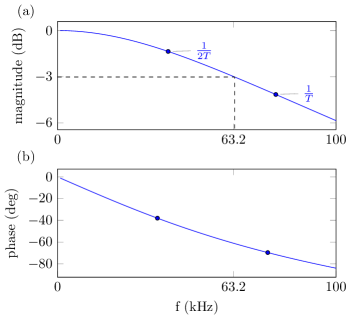
Figure 4: Bode plot of the electronic filter for a dc-voltage. The inverse transport time $1/T$ is on the order of the cut off frequency of the electronic filters. The horizontal axis of the plot is scaled linear.

One possibility to apply fast step function-like potential changes to trap electrodes is the usage of switches located next to the trap that are switching between different voltage channels at a point where the low-pass filtering has already been applied Alonso et al. (2013).

An other solution is to calculate backwards source voltages $\tilde{U}(t_{i})$ such that one gets the desired voltages $U(t_{i})$ after the low pass filter. A serious downside of this method is that the maximal possible voltage change $\delta U$ at the electrodes is not only limited by the maximal possible voltage change $\delta\tilde{U}$ of the source, but is also a function of the history of applied voltages. To ensure realizable voltage sequences one needs to reduce the value of $\delta U$ in (5) such that in any case it could be produced by a voltage change of $\delta\tilde{U}$ at the voltage source for all voltage histories. This precaution — if realizable at all — reduces the available dynamics of the voltage source and in consequence the speed of ion transport operations.

We circumvent this problem by incorporating the characteristics of the electronic filters directly in the calculation of the potentials for all steps of the trajectory.

Our electronic filters are constructed by a series of three stages of first order RC low-pass filters and the trap capacitance itself: The first stage terminates our homebuilt programmable voltage source, followed by two stages located next to vacuum interface. Figure 4 shows the corresponding Bode plot. The magnitude of the amplitude in this plot is determined indirectly by measuring the amplitude of a sinus signal parallel to the trap and fitting the capacitances of the trap electrodes. The phase shift is calculated using the obtained model. The cut-off frequency of the system is $63.2\text{\,}\mathrm{kHz}\text{/}$ and on the order of the inverse ion transport time $1/T$, showing the necessity to take the filter characteristics into account.

From the electronic circuit we obtain the transfer function $G(s)=\mathcal{L}\{U(t)\}/\mathcal{L}\{\tilde{U}(t)\}$ between source voltage and electrode voltage as quotient of the two-sided Laplace transforms of input and output voltages with the complex parameter $s=i\omega$ Oppenheim and Schafer (1989). From $G(s)$ a time discrete rational state space transfer function

$$\sum_{n=0}^{n_{a}}a_{n}U_{i-n}=\sum_{n=1}^{n_{b}}b_{n}\tilde{U}_{i-n}$$ (6)

can be calculated that connects input and output voltages of the electronic filter Oppenheim and Schafer (1989) ($b_{0}$ is equal zero such that ${U}_{i}$ is independent of $\tilde{U}_{i}$ — the output is one step behind the input). $n_{a}$ and $n_{b}$ are called feedback and feedforward filter orders and are equal $4$ in our case. The value of the coefficients $a_{n}$ and $b_{n}$ are determined by the resistors and capacitors used.

Solving (6) for $U_{i}$ and substituting $\tilde{U}_{i}=\tilde{U}_{i-1}-\delta\tilde{U}$ resp. $\tilde{U}_{i}=\tilde{U}_{i-1}+\delta\tilde{U}$ yields the range of the next possible electrode voltages and thus condition (5) is replaced by:

$$U_{i}\lessgtr\frac{1}{a_{0}}\left(b_{1}(\tilde{U}_{i-1}\pm\delta\tilde{U})+\sum_{n=2}^{n_{b}}b_{n}\tilde{U}_{i-n}-\sum_{n=1}^{n_{a}}a_{n}U_{i-n}\right)$$ (7)

I.2 Micromotion minimization

The trapping potential simulations assume a perfectly fabricated and assembled trap and zero electric stray fields. Deviations from these assumptions require small offset voltages to match the position of the potentials dc- and rf-null. We determine two sets of optimized offset voltages $\Delta U^{(j)}_{1}$ and $\Delta U^{(j)}_{L}$ for the start and final position of the ion trajectory using the method described by Gloger et al. (2015). For ion positions between these points we are using linearly interpolated values for the offset voltages $\Delta U_{i}^{(j)}$. The offset voltages are added to the voltages obtained from the potential optimization.

In order to guarantee that the total voltage $\overline{U}_{i}=U_{i}+\Delta U_{i}$ including the offset voltages for micromotion minimization is achievable, the voltage limits (7) for the potential problem of the ideal trap have to be adjusted by $-\Delta U_{i}$:

$$U_{i}\lessgtr\frac{1}{a_{0}} \left(b_{1}(\tilde{U}_{i-1}\pm\delta\tilde{U})+\sum_{n=2}^{n_{b}}b_{n}\tilde{U}_{i-n}-\right.$$

$$\left.\sum_{n=1}^{n_{a}}a_{n}U_{i-n}-\Delta U_{i}\right)$$ (8)

The electrostatic problem can now be solved for the electrode voltages $U_{i}$ and using (6) suitable source voltages $\tilde{\overline{U}}_{i-1}$ including the filter characteristics and micromotion compensation can be calculated:

$$\tilde{\overline{U}}_{i-1}=\frac{1}{b_{1}}\left(\sum_{n=0}^{n_{a}}a_{n}\overline{U}_{i-n}-\sum_{n=2}^{n_{b}}b_{n}\tilde{\overline{U}}_{i-n}\right)$$ (9)

The optimization algorithm can be fine tuned by adding several additional constraints to the optimization problem. We limit the voltage difference between voltage source and electrodes by implementing an additional condition $\tilde{\overline{U}}-\overline{U}=0$ for the potential optimization problem with a small weight. Additionally we favor similar voltages for the transport in both directions ($U^{(j)}_{A\rightarrow B}(r_{i})-U^{(j)}_{B\rightarrow A}(r_{i})=0$) to achieve a closed voltage loop, that is needed for an easy scaling of transport operations. For this condition we use a weight factor that relaxed the condition for coordinates between $A$ and $B$.

Supplemental Material II Transport fidelity

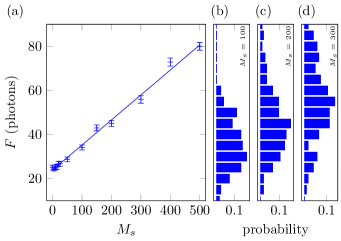
Figure 5: (a) The mean fluorescence $F$ is a linear function of the number $M_{s}$ of intentionally skipped transport operations. A linear fit yields $0.113(4)$ for the slope and $23.9(6)$ for the offset of the curve. (b)-(d) Three sample fluorescence histograms ($M_{s}=100,200,300$) that were used to extract $F$. Each histogram holds data of 125 single experiment runs.

We drive the $\ket{S_{\nicefrac{{1}}{{2}}}}-\ket{P_{\nicefrac{{1}}{{2}}}}$ dipole transition by a single laser. So the fluorescence rate on this transition is higher for the ¹⁷²Yb⁺ isotope without hyperfine and Zeeman splitting compared to the ¹⁷¹Yb⁺ ion where only a fraction of the $12$ possible transitions between $S_{\nicefrac{{1}}{{2}}}$ and $P_{\nicefrac{{1}}{{2}}}$ are driven in parallel. To profit from the better detection statistics we perform this part of the experiment using ¹⁷²Yb⁺.

To calibrate the measurements of the absent ion we perform the experiment with $M_{s}$ transport operations $A\rightarrow B\rightarrow A$ skipped by intent (see Fig. 5). As the ion is detected at position $A$ when it should have been transported to position $B$, the detected fluorescence $F$ is increasing with $M_{s}$. The expected average photon count $F$ during an experiment of $M$ consecutive transfer operations is given by $F(M_{s})=M_{s}F_{b}+(M-M_{s})F_{d}$, with $F_{b}$ and $F_{d}$ being the average number of photons per detection flash collected from a present (bright) and absent (dark) ion respectively. If a fraction $f_{s}$ of transport operations $A\rightarrow B$ is failing, $f_{s}(M-M_{s})$ additional bright and $f_{s}(M-M_{s})$ fewer dark events are expected. For the direction $B\rightarrow A$ one has to adjust $F$ by $f_{s}M_{s}F_{d}$ and $-f_{s}M_{s}F_{b}$ accordingly. So the expected total photon number is

$$F(M_{s})= F_{b}[M_{s}+f_{s}(M-2M_{s})]+$$

$$F_{d}[(M-M_{s})-f_{s}(M-2M_{s})]\,.$$ (10)

In an additional run without an ion loaded to the trap we measured the average photon number of an absent ion per flash to be $F_{d}=$23.5(3)$/M$. From a fit of (10) to the data, we find the probability for transporting the ion as intended per shuttling event to be $1-f_{s}=0.998\left({}^{+2}_{-3}\right)$ — corresponding to $8\left({}^{+12}_{-8}\right)$ out of $4000$ transport operations failing.

Supplemental Material III Interpretation of the observed decoherence

The measured internal state fidelity upon transport of $0.999994\left({}^{+6}_{-7}\right)$ is compatible with unity within one standard deviation. Therefore, an unambiguous attribution of the Ramsey fringes’ loss of contrast to particular sources of decoherence is not possible. Nevertheless, several processes can be ruled out as sources of decoherence from the following discussion.

As the states of the hyperfine qubit are, for all practical purposes considered here, not subject to spontaneous emission, the mechanism leading to decoherence is dephasing: During the precession time the qubit state accumulates a phase $\Delta\varphi=\Delta\nu~{}t_{p}$ relative to the driving field of the $\pi/2$ pulses, where $\Delta\nu$ describes a stochastically varying detuning of this field from the qubit transition.

Assuming a normal distribution

$$\rho(\Delta\varphi)=\frac{1}{\sqrt{2\pi}\sigma_{\varphi}}e^{-\frac{(\Delta\varphi)^{2}}{2\sigma_{\varphi}^{2}}}$$ (11)

of $\Delta\varphi$ over all measurements, a convolution of the Ramsey fringe $p_{b}(\varphi)=B+A\sin(\varphi-\Phi)$ with $\Delta\varphi$ results in a contrast reduction by a factor of $\exp(-\sigma_{\varphi}^{2}/2)$. The contrast decay observed in this paper due to one qubit transport operation yields $\sigma_{\varphi}=2\pi\times 6\left({}^{+8}_{-6}\right)\times 10^{-4}$.

The magnetic field at the position of the ion transport is $B=$640\text{\,}\mathrm{\SIUnitSymbolMicro T}\text{/}$$ and it’s gradient in the direction of the ion transport $dB/dx=$10.6\text{\,}\mathrm{mT}\text{/}\mathrm{m}$$. The magnetic field sensitivity of the qubit is $d\nu/dB=$39.7\text{\,}\mathrm{MHz}\text{/}\mathrm{T}$$. These values combined yield a position sensitivity of the qubit transition of $d\nu/dx=$397\text{\,}\mathrm{kHz}\text{/}\mathrm{m}$$ in the direction of transport.

The repeated measurements of the Ramsey fringes with $2$ and $4000$ transport operations are carried out interleaved, every single measurement being synchronized to the phase of the power line. Therefore we exclude an additional loss of contrast of the measurement using $4000$ transport operations due to fluctuations of the magnetic field.

The electric currents caused by the transport potentials are much too small to cause additional magnetic fields large enough to explain a dephasing on the order of $10^{-4}$ per transport. Furthermore, as the transport potentials are changed in a deterministic fashion, the accompanying currents would result in a deterministic change of the magnetic field that wouldn’t cause dephasing. So even qualitatively a dephasing could only be caused by electronic noise components, not by the potentials themselves.

Assuming a perfectly static magnetic field, a stochastic distribution of the transport trajectories with a width of $\sigma_{x}$ would lead to dephasing due to the magnetic gradient and the qubits residual magnetic field sensitivity. With

$$\sigma_{x}=\sigma_{\varphi}\left(2\pi t\frac{d\nu}{dx}\right)^{-1}$$ (12)

and the duration of a single transport operation $t=$12.8\text{\,}\mathrm{\SIUnitSymbolMicro s}\text{/}$$, the uncertainty in the transport trajectories required to produce the observed phase distribution would be $\sigma_{x}=110\left({}^{+50}_{-110}\right)\mu\text{m}$. From our observations of the ion after transport, we can exclude any value of $\sigma_{x}$ larger than a few $\mu\text{m}$. Therefore, possible stochastic variations of the ion transport trajectory do not limit the measured internal state fidelity.

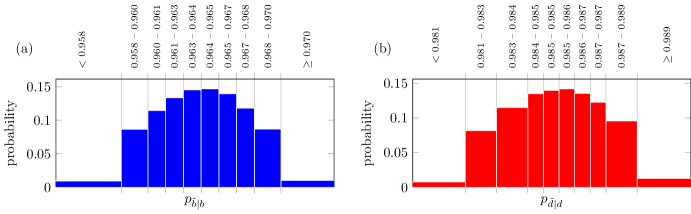
Figure 6: State detection fidelities for $M=4000$ transport operations. The histograms are generated by repeatedly selecting random sets from the calibration measurements. The bin edges are selected such that the number of total events in the single bins are closely matching while avoiding binning effects at the same time. The first and last intervals are only shown in part.

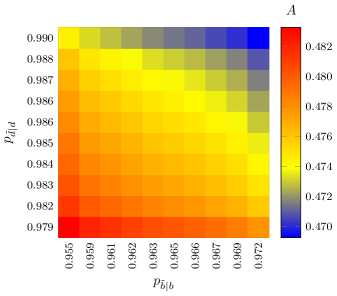
Figure 7: The amplitude $A$ of the fitted Ramsey fringes depends on the assumed state identification probabilities $p_{\tilde{b}|b}$ and $p_{\tilde{d}|d}$. If the states can be identified with lower probability the likelihood analysis scales the measurement data accordingly towards the extreme values $0$ and $1$ resulting in a higher amplitude. To account for this effect the data analysis is carried out for 100 combinations of $p_{\tilde{b}|b}$ and $p_{\tilde{d}|d}$ with similar likelihoods.

None of the possible sources of dephasing discussed in this section is large enough to explain the observed loss of internal state fidelity. We like to stress that within the calculated error budget a finding of smaller transport induced coherence loss is also not to be ruled out.

Supplemental Material IV Bootstrap analysis of the calibration data

The state identification probabilities $p_{\tilde{b}|b}$ and $p_{\tilde{d}|d}$ are parameters of the data analysis. We estimate their uncertainties by applying the bootstrapping resampling method Efron and Tibshirani (1994) to the calibration data. Figure 6 shows the distributions of $p_{\tilde{b}|b}$ and $p_{\tilde{d}|d}$ obtained from $10000$ resampling runs. Binning of the data is done such that every of the $10$ bins represents almost the same fraction $w(p_{\tilde{b}|b})$ ($w(p_{\tilde{d}|d})$) of results. So every combination of $p_{\tilde{b}|b}$ and $p_{\tilde{d}|d}$ has almost the same significance of $w(p_{\tilde{b}|b},p_{\tilde{d}|d})=w(p_{\tilde{b}|b})w(p_{\tilde{d}|d})\approx 1/100$.

The maximum likelihood fit of the Ramsey fringes is carried out for every such combination using the weighted mean for $p_{\tilde{b}|b}$ and $p_{\tilde{d}|d}$ in the corresponding interval and the resulting profile likelihood function $\mathcal{L}_{M}(A|p_{\tilde{b}|b},p_{\tilde{d}|d})$ of the parameter $A$ is calculated. Figure 7 shows the most likely amplitudes for each combination of the state identification probabilities. If one assumes smaller state identification probabilities the amplitude is generally estimated to be higher.

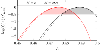
Figure 8: Log likelihoods for the amplitude of the Ramsey fringes with $2$ and $4000$ transfer operations. The $68\%$ confidence intervals (shaded) are overlapping. The log likelihoods are calculated by adding up the likelihoods $\mathcal{L}_{M}(A|p_{\tilde{b}|b},p_{\tilde{d}|d})$ obtained by data analysis for different pairs of $p_{\tilde{b}|b}$ and $p_{\tilde{d}|d}$. For comparison the dashed curves are showing the one pair of likelihoods $\mathcal{L}_{M}(A|p_{bb},p_{dd})$ that is determined from the Ramsey fringes in main text, Fig. 2.

Figure 8 shows the log likelihood function $\mathcal{L}_{M}(A)$ obtained by summing up the single likelihoods

$$\mathcal{L}_{M}(A)=\sum_{p_{\tilde{b}|b},p_{\tilde{d}|d}}w(p_{\tilde{b}|b},p_{\tilde{d}|d})\mathcal{L}_{M}(A|p_{\tilde{b}|b},p_{\tilde{d}|d})$$ (13)

Again one can see that the most likely amplitude of the Ramsey fringes for more transport operations is slightly smaller. The $1\sigma$ confidence interval of the amplitude for $M=2$ and $M=4000$ are overlapping. By comparing the likelihoods obtained with and without usage of the bootstrapped distributions $p_{\tilde{b}|b}$ and $p_{\tilde{d}|d}$ one can see that the inclusion of this statistical error source is broadening and slightly shifting the maximum of the calculated likelihoods.

Supplemental Material V Preparation errors

The identification probabilities $p_{\tilde{b}|b}$ and $p_{\tilde{d}|d}$ are determined under the assumption that the bright and dark states can be prepared with unit fidelity.

If the states $\ket{0}$ and $\ket{1}$ are not correctly prepared, the identification probabilities are systematically biased towards lower values. The usage of low biased values in the data analysis will result in systematically overestimated fringe contrasts (compare Fig. 7). If the state preparation (${\mathcal{F}}_{p}$) and $\pi$ pulse (${\mathcal{F}}_{\pi}$) fidelities are known, unbiased values $\overline{p}_{\tilde{b}|b}$ and $\overline{p}_{\tilde{d}|d}$ can be calculated as

$$\overline{p}_{\tilde{b}|b} =\frac{p_{\tilde{d}|d}(2{\mathcal{F}}_{p}{\mathcal{F}}_{\pi}-{\mathcal{F}}_{p}-{\mathcal{F}}_{\pi})+{\mathcal{F}}_{p}(1-2{\mathcal{F}}_{\pi}-p_{\tilde{b}|b})+{\mathcal{F}}_{\pi}}{(1-2{\mathcal{F}}_{p}){\mathcal{F}}_{\pi}}$$ (14)

$$\overline{p}_{\tilde{d}|d} =\frac{p_{\tilde{d}|d}(-2{\mathcal{F}}_{p}{\mathcal{F}}_{\pi}+{\mathcal{F}}_{p}+{\mathcal{F}}_{\pi}-1)+({\mathcal{F}}_{p}-1)(p_{\tilde{b}|b}-1)}{(1-2{\mathcal{F}}_{p}){\mathcal{F}}_{\pi}}$$ (15)

The statistics approach used in this paper includes the effect of the imperfect identification probabilities. By connecting identified states to projected states, the probability densities for a given measurement result are effectively rescaled.

An alternative approach to take the limited state identification probabilities into consideration is to first apply a linear transformation

$$\underbrace{\left(\begin{array}[]{c}b\\ d\end{array}\right)}_{{\mathbf{r}}}={\underbrace{\left(\begin{array}[]{cc}p_{\tilde{b}|b}&1-p_{\tilde{d}|d}\\ 1-p_{\tilde{b}|b}&p_{\tilde{d}|d}\\ \end{array}\right)}_{M(p_{\tilde{b}|b},p_{\tilde{d}|d})}}^{-1}\underbrace{\left(\begin{array}[]{c}\tilde{b}\\ \tilde{d}\end{array}\right)}_{{\mathbf{\tilde{r}}}}$$ (16)

to the identified measurement results ${\mathbf{\tilde{r}}}=(\tilde{b},\tilde{d})^{T}$ and then employ the beta probability function on the rescaled measurement results $b$ and $d$. The transformation matrix $M(p_{\tilde{b}|b},p_{\tilde{d}|d})$ is determined by the identification probabilities. Even though this approach distorts the probability density $\rho(p_{b}|\tilde{b},N)$ and systematically underestimates statistical errors by not taking into account the broadening of the distribution due to the stochastic interpretation of projected states, described by binomial distributions with probabilities $p_{\tilde{b}|b}$ and $p_{\tilde{d}|d}$, the most likely value for the probability density of a measured state remains unbiased.

Using this simplified method we discuss the effects of biased detection probabilities on the bias for determination of the internal state fidelity ${\mathcal{F}}$:

If $\overline{A}$ and $\overline{B}$ are the amplitude and offset of the Ramsey fringe, an outcome

$${\mathbf{\overline{r}}}_{\text{max}}=N\left(\begin{array}[]{c}\overline{B}+\overline{A}\\ \overline{B}-\overline{A}\end{array}\right)$$ (17)

at the fringe maximum for $N$ measurements is to be expected, a reading of ${\mathbf{\overline{r}}}_{\text{min}}=N(\overline{B}-\overline{A},\overline{B}+\overline{A})^{T}$ at the minimum respectively. Due to the limited state identification probabilities these measurement outcomes will be identified as ${\mathbf{\tilde{r}}}_{\text{max}}=M(\overline{p}_{\tilde{b}|b},\overline{p}_{\tilde{d}|d}){\mathbf{\overline{r}}}_{\text{max}}$ and ${\mathbf{\tilde{r}}}_{\text{min}}=M(\overline{p}_{\tilde{b}|b},\overline{p}_{\tilde{d}|d}){\mathbf{\overline{r}}}_{\text{min}}$. A transformation according to (16) based on biased state identification probabilities yields ${\mathbf{r}}_{\text{min/max}}=[M({p}_{\tilde{b}|b},{p}_{\tilde{d}|d})]^{-1}M(\overline{p}_{\tilde{b}|b},\overline{p}_{\tilde{d}|d}){\mathbf{\overline{r}}}_{\text{min/max}}$. Using (14) and (15) one finds, that the factor between unbiased (${\mathbf{\overline{r}}}$) and biased (${\mathbf{r}}$) values depends on the state preparation and $\pi$ pulse fidelities only and does not depend on $p_{\tilde{b}|b}$ or $p_{\tilde{d}|d}$. The biased amplitude $A$ of the Ramsey fringes is given by half the difference of bright events in the maximum and minimum of the Ramsey fringe $\frac{1}{2}({\mathbf{r}}_{\text{max}}-{\mathbf{r}}_{\text{min}})_{1}$:

$$A =\frac{1}{2}\left\{[M({p}_{\tilde{b}|b},{p}_{\tilde{d}|d})]^{-1}M(\overline{p}_{\tilde{b}|b},\overline{p}_{\tilde{d}|d})\frac{{\mathbf{\overline{r}}}_{\text{max}}-{\mathbf{\overline{r}}}_{\text{min}}}{N}\right\}_{1}$$

$$=\frac{\overline{A}}{{\mathcal{F}}_{\pi}(2{\mathcal{F}}_{p}-1)}$$ (18)

The amplitude is biased towards higher values, but for the determination of the internal state fidelity during ion transport ${\mathcal{F}}=\sqrt[4000-2]{A_{2}/A_{4000}}$ only the ratio of the amplitudes for $M=2$ and $M=4000$ is of interest and the factor $[{\mathcal{F}}_{\pi}(2{\mathcal{F}}_{p}-1)]^{-1}$ in (18) cancels.

As noted before the linear transformation used in the reasoning above distorts the probability density function and an exact statistical treatment of the problem reintroduces a small dependence of the fidelity ${\mathcal{F}}$ on the state identification probabilities. We assume a preparation fidelity of ${\mathcal{F}}_{p}>1-$1\text{\times}{10}^{-4}$$ and a fidelity of the fault tolerant BB1RWR $\pi$ pulse of ${\mathcal{F}}_{\pi}>1-$1.3\text{\times}{10}^{-4}$$. The corresponding maximal bias of the identification probabilities are $-9.5\text{\times}{10}^{-5}$ ($p_{\tilde{b}|b}$) and $-2.2\text{\times}{10}^{-4}$ ($p_{\tilde{d}|d}$). A data analysis assuming these biases yields numerically insignificant changes ($-$2.4\text{\times}{10}^{-8}$$) to the overall result for the internal state fidelity during ion transport. This still holds when infidelities of ${\mathcal{F}}_{\pi}$ and ${\mathcal{F}}_{p}$ of $1\text{\times}{10}^{-3}$ are assumed ($-$2.2\text{\times}{10}^{-7}$$).

References

- Blatt and Wineland (2008) R. Blatt and D. Wineland, Nature 453, 1008 (2008).
- Kielpinski et al. (2002) D. Kielpinski, C. Monroe, and D. J. Wineland, Nature 417, 709 (2002).
- Svore et al. (2006) K. M. Svore, A. V. Aho, A. W. Cross, I. Chuang, and I. L. Markov, in Computer, Vol. 39 (IEEE Computer Society, 2006) pp. 74–83.
- Monroe et al. (2014) C. Monroe, R. Raussendorf, A. Ruthven, K. R. Brown, P. Maunz, L.-M. Duan, and J. Kim, Phys. Rev. A 89, 022317 (2014).
- Lekitsch et al. (2017) B. Lekitsch, S. Weidt, A. G. Fowler, K. Mølmer, S. J. Devitt, C. Wunderlich, and W. K. Hensinger, Science Advances 3, e1601540 (2017).
- Shor (1995) P. W. Shor, Phys. Rev. A 52, R2493 (1995).
- Steane (1996) A. Steane, Proceedings: Mathematical, Physical and Engineering Sciences 452, 2551 (1996).
- Knill (2010) E. Knill, Nature 463, 441 (2010).
- Brown et al. (2011) K. R. Brown, A. C. Wilson, Y. Colombe, C. Ospelkaus, A. M. Meier, E. Knill, D. Leibfried, and D. J. Wineland, Phys. Rev. A 84, 030303 (2011).
- Ballance et al. (2016) C. J. Ballance, T. P. Harty, N. M. Linke, M. A. Sepiol, and D. M. Lucas, Phys. Rev. Lett. 117, 060504 (2016).
- Piltz et al. (2014) C. Piltz, T. Sriarunothai, A. F. Varón Rojas, and C. Wunderlich, Nature Communications 5, 4679 (2014).
- Burrell et al. (2010) A. H. Burrell, D. J. Szwer, S. C. Webster, and D. M. Lucas, Phys. Rev. A 81, 040302 (2010).
- Benhelm et al. (2008) J. Benhelm, G. Kirchmair, C. F. Roos, and R. Blatt, Nat Phys 4, 463 (2008).
- Harty et al. (2016) T. P. Harty, M. A. Sepiol, D. T. C. Allcock, C. J. Ballance, J. E. Tarlton, and D. M. Lucas, Phys. Rev. Lett. 117, 140501 (2016).
- Gaebler et al. (2016) J. P. Gaebler, T. R. Tan, Y. Lin, Y. Wan, R. Bowler, A. C. Keith, S. Glancy, K. Coakley, E. Knill, D. Leibfried, and D. J. Wineland, Phys. Rev. Lett. 117, 060505 (2016).
- Weidt et al. (2016) S. Weidt, J. Randall, S. C. Webster, K. Lake, A. E. Webb, I. Cohen, T. Navickas, B. Lekitsch, A. Retzker, and W. K. Hensinger, Phys. Rev. Lett. 117, 220501 (2016).
- Monz et al. (2009) T. Monz, K. Kim, W. Hänsel, M. Riebe, A. S. Villar, P. Schindler, M. Chwalla, M. Hennrich, and R. Blatt, Phys. Rev. Lett. 102, 040501 (2009).
- Piltz et al. (2016) C. Piltz, T. Sriarunothai, S. S. Ivanov, S. Wölk, and C. Wunderlich, Science Advances 2, e1600093 (2016).
- Johanning (2016) M. Johanning, Applied Physics B 122, 71 (2016).
- Lin et al. (2009) G.-D. Lin, S.-L. Zhu, R. Islam, K. Kim, M.-S. Chang, S. Korenblit, C. Monroe, and L.-M. Duan, Europhysics Letters 86, 60004 (2009).
- Hucul et al. (2015) D. Hucul, I. V. Inlek, G. Vittorini, C. Crocker, S. Debnath, S. M. Clark, and C. Monroe, Nat Phys 11, 37 (2015).
- Rowe et al. (2002) M. A. Rowe, A. Ben-Kish, B. Demarco, D. Leibfried, V. Meyer, J. Beall, J. Britton, J. Hughes, W. M. Itano, B. Jelenković, C. Langer, T. Rosenband, and D. J. Wineland, Quantum Info. Comput. 2, 257 (2002).
- Hensinger et al. (2006) W. K. Hensinger, S. Olmschenk, D. Stick, D. Hucul, M. Yeo, M. Acton, L. Deslauriers, C. Monroe, and J. Rabchuk, Applied Physics Letters 88, 034101 (2006).
- Blakestad et al. (2009) R. B. Blakestad, C. Ospelkaus, A. P. VanDevender, J. M. Amini, J. Britton, D. Leibfried, and D. J. Wineland, Phys. Rev. Lett. 102, 153002 (2009).
- Singer et al. (2010) K. Singer, U. Poschinger, M. Murphy, P. Ivanov, F. Ziesel, T. Calarco, and F. Schmidt-Kaler, Rev. Mod. Phys. 82, 2609 (2010).
- Bowler et al. (2012) R. Bowler, J. Gaebler, Y. Lin, T. R. Tan, D. Hanneke, J. D. Jost, J. P. Home, D. Leibfried, and D. J. Wineland, Phys. Rev. Lett. 109, 080502 (2012).
- Walther et al. (2012) A. Walther, F. Ziesel, T. Ruster, S. T. Dawkins, K. Ott, M. Hettrich, K. Singer, F. Schmidt-Kaler, and U. Poschinger, Phys. Rev. Lett. 109, 080501 (2012).
- de Clercq et al. (2016) L. E. de Clercq, H.-Y. Lo, M. Marinelli, D. Nadlinger, R. Oswald, V. Negnevitsky, D. Kienzler, B. Keitch, and J. P. Home, Phys. Rev. Lett. 116, 080502 (2016).
- Chiaverini et al. (2005) J. Chiaverini, R. B. Blakestad, J. Britton, J. D. Jost, C. Langer, D. Leibfried, R. Ozeri, and D. J. Wineland, Quantum Information and Computation 5, 419 (2005).
- Note (1) We assume gaussian errors of the reported Ramsey fringe contrasts and calculate the fidelity as , where is the contrast before and after transport operations.
- Vitanov et al. (2015) N. V. Vitanov, T. F. Gloger, P. Kaufmann, D. Kaufmann, T. Collath, M. Tanveer Baig, M. Johanning, and C. Wunderlich, Phys. Rev. A 91, 033406 (2015).
- Kaufmann et al. (2012) D. Kaufmann, T. Collath, M. T. Baig, P. Kaufmann, E. Asenwar, M. Johanning, and C. Wunderlich, Applied Physics B 107, 935 (2012).
- Schulz et al. (2006) S. Schulz, U. Poschinger, K. Singer, and F. Schmidt-Kaler, Fortschritte der Physik 54, 648 (2006).
- Schulz et al. (2008) S. A. Schulz, U. Poschinger, F. Ziesel, and F. Schmidt-Kaler, New Journal of Physics 10, 045007 (2008).
- Baig et al. (2013) M. T. Baig, M. Johanning, A. Wiese, S. Heidbrink, M. Ziolkowski, and C. Wunderlich, Review of Scientific Instruments 84, 124701 (2013).
- Blakestad et al. (2011) R. B. Blakestad, C. Ospelkaus, A. P. VanDevender, J. H. Wesenberg, M. J. Biercuk, D. Leibfried, and D. J. Wineland, Phys. Rev. A 84, 032314 (2011).
- Torrontegui et al. (2011) E. Torrontegui, S. Ibáñez, X. Chen, A. Ruschhaupt, D. Guéry-Odelin, and J. G. Muga, Phys. Rev. A 83, 013415 (2011).
- Wölk et al. (2015) S. Wölk, C. Piltz, T. Sriarunothai, and C. Wunderlich, Journal of Physics B: Atomic, Molecular and Optical Physics 48, 075101 (2015).
- Cummins et al. (2003) H. K. Cummins, G. Llewellyn, and J. A. Jones, Phys. Rev. A 67, 042308 (2003).
- Efron and Tibshirani (1994) B. Efron and R. Tibshirani, An Introduction to the Bootstrap (Taylor & Francis, 1994).
- Mintert and Wunderlich (2001) F. Mintert and C. Wunderlich, Phys. Rev. Lett. 87, 257904 (2001).
- Alonso et al. (2013) J. Alonso, F. M. Leupold, B. C. Keitch, and J. P. Home, New Journal of Physics 15, 023001 (2013).
- Oppenheim and Schafer (1989) A. V. Oppenheim and R. W. Schafer, Disrete-Time Signal Processing (Prentice-Hall, Inc., 1989).
- Gloger et al. (2015) T. F. Gloger, P. Kaufmann, D. Kaufmann, M. T. Baig, T. Collath, M. Johanning, and C. Wunderlich, Phys. Rev. A 92, 043421 (2015).