Empirical analysis and agent-based modeling of the Lithuanian parliamentary elections

Abstract

In this contribution we analyze a parties’ vote share distribution across the polling stations during the Lithuanian parliamentary elections of 1992, 2008 and 2012. We find that the distribution is rather well fitted by the Beta distribution. To reproduce this empirical observation we propose a simple multi-state agent-based model of the voting behavior. In the proposed model agents change the party they vote for either idiosyncratically or due to a linear recruitment mechanism. We use the model to reproduce the vote share distribution observed during the election of 1992. We discuss model extensions needed to reproduce the vote share distribution observed during the other elections.

1 Introduction

While any individual vote is equally important to determine the outcome of an election, the probability for a single vote to decide the outcome is extremely small. As utility of casting a vote in this context seems to be small and as there is at least a minor associated cost, it seems that a rational choice would be simply not to vote. Yet this simplistic context may be further extended to provide a sound reasoning for why people vote. Some argue that people vote to show a support for the political system [1] or to avoid a risk of regret [2], there might also be a social cost for abstension [3]. Some of the aforementioned works as well as numerous other earlier game theoretic approaches, such as [4, 5, 6], had shown promise that game theoretic voting models would soon provide rich and sophisticated explanation for the voting behavior. Yet further research have shown that general game theoretic models of the voting behavior with pure Nash equilibrium, and even mixed Nash equilibrium, might be impossible unless under certain specific conditions [7, 8, 9]. But people are rarely well informed and ideally rational, as they are not homo economicus nor are they Laplace’s demons, [10, 11, 12].

The above context provides a good reasoning to consider the modeling of the voting behavior from the perspective of psychology [13, 14, 15, 16, 17, 18, 19, 20]. The main drawback of these psychologically motivated models is that they usually are rather complicated, at least when compared with game theoretic models, hard to implement and understand the obtained results. Also usually these models involve a large number of parameters, which may lead to overfitting the data or different parameter sets providing similar results. Notably recently a psychologically motivated model was successfully used to predict the Polish election of 2015 [17, 19].

Another possible approach to the modeling of the voting behavior has its roots in statistical physics. This perspective could be neatly summarized by quoting the Boltzmann’s molecular chaos hypothesis [21]:

The molecules are like so many individuals, having the most various states of motion, and the properties of gases only remain unaltered because the number of these molecules which on the average have a given state of motion is constant.

During the last three decades physicists have approached social and economic systems from this perspective, looking for universal laws and important statistical patterns, while proposing simple theoretical models to explain the empirical observations. This effort by a numerous more or less prominent physicists became what is now known as sociophysics and econophysics [22, 23, 24, 25, 26, 27]. The opinion dynamics, and the voting behavior as a proxy of opinion, is still one of the major topics in sociophysics [28, 29, 25, 26, 30, 27].

This paper contributes to the understanding and describtion of the voting behavior from a couple of different point of views. First of all Lithuania is a young democratic nation and the analysis of the Lithuanian parliamentary elections’ data sets seems interesting in the context of similar analyses carried out on the data sets gathered in the mature democratic nations, such as Brazil, England, Germany, France, Finland, Norway or Switzerland [31, 32, 33, 34, 35]. In the political science and sociological literature one would find numerous previous approaches to the Lithuanian parliamentary elections, e.g., [36, 37, 38, 39, 40]. Yet most of these approaches had a quite different perspective, most of these papers discuss general electoral trends in the context of social, demographic and economic changes. For this kind of discussion a highly aggregated (e.g., on a municipal district level) data sets prove to be sufficient, while in this paper we will consider the data on the smallest scale available (polling station level).

Another key contribution of this paper is a simple agent-based model, which is used to explain the statistical patterns uncovered during the empirical analysis. The proposed model is built upon a two-state herding model originally proposed by Kirman in [41]. In the recent years the two-state herding model was quite frequently and rather successfully applied to reproduce the statistical patterns observed in the empirical data of the financial markets [42, 43, 44, 45, 46, 47, 48]. In this paper we extend the two-state herding model to allow the agents to switch between more than two states. We discuss the similarity between the proposed model and the well known Voter model [49, 50, 51, 52, 53, 54].

Our approach is unique in a sense that we consider reproducing the parties’ vote share distribution observed in the Lithuanian parliamentary elections. In the previous literature there was only a single attempt to model, and predict, popular vote (aggregated vote share) in the Lithuanian parliamentary elections using regression model, see [55]. Numerous previous sociophysics papers have mainly ignored the vote share distribution, likely due to belief that the vote share distribution reflects electoral sensitivity to the policies promoted by the parties and less to the endogenous interactions between the voters (a similar argument is given in [31]). To some extent this belief is supported by game theoretic models, see [5, 6]. Notably there were a couple of sociophysics papers considering two-state agent-based models of the voting behavior, e.g., voting for or against certain proposals in a referendum [29]. It is interesting to note that recently the binary models considered in [29] were used to construct a simple financial market model [56], while we start from the financial market model[47] and move towards the model of the voting behavior. While the vote share distribution was mainly ignored in the previous sociophysics papers, the other statistical patterns arising during the many different elections were considered for the empirical analysis and modeling: a branching process model was proposed to reproduce the individual politician, nominated via open party list, vote share distribution [31], a network model was used to explain how people decide whether to take part in the municipal elections [34], a diffusive model for the turn-out was proposed in [33, 35]. One of a more similar approaches was taken by [57], in which a generative model was proposed to reproduce the rank-size distribution of parties’ vote share. Another similar approach, taken by [54], considered the vote share distribution observed in the elections of House of Representatives in Japan. Latter approach [54] also used a mean-field Voter model to explain the empirical observations.

This paper is organized as follows. In Section 2 we discuss the Lithuanian parliamentary election system as well as carry out the empirical analysis. Next, in Section 3, we briefly introduce the two-state herding model and extend it to account for the multiple states. Afterwards, in Section 4, we apply the extended model to reproduce the statistical patterns uncovered during the empirical analysis. Finally we end the paper with a discussion (see Section 5).

2 Empirical analysis of the data from the Lithuanian parliamentary elections

Let us start by discussing the parliamentary voting system used in Lithuania. Lithuanian parliamentary elections are held every $4$ years. During every election all of the $141$ parliamentary seats are distributed using two-tier voting system. Namely, $71$ seats in the parliament are taken by elected district representatives (there are $71$ electoral districts in total), while the other $70$ seats are distributed according to the popular vote among the parties that received more than $5\%$ of the popular vote. In other words, each individual voter is able to vote for a single candidate to represent his electoral district (the two round voting system is used) and for an open party list (listing up to $5$ individuals from that list). Every electoral district has multiple polling stations (their number varies over the years), which further subdivide the electoral districts. Every eligible voter is assigned to a single polling station based on location of their residence. Each of the polling stations may have widely different number of the assigned voters – some of the smallest polling stations have as few as $100$ assigned voters, while the largest have up to $7000$ assigned voters.

In this paper we consider only votes cast for the open party lists in each of the local polling stations. We do not analyze ranking of the individuals on the party lists (similar analysis was carried out in, e.g., [31]), voting for the representative of electoral district (similar data was previously considered in, e.g., [57, 54]) nor turnout rates (modeling and analysis of which was previously considered in, e.g., [33, 35]). We ignore votes cast in the polling stations abroad or votes cast by post. In the analysis that follows we consider only parties that were elected to the parliament (total vote share larger thant $5\%$), while all other less succesful parties were combined into a single party, which we have labeled as the “Other” party.

In this paper we consider the three data sets from the Lithuanian parliamentary elections of 1992, 2008 and 2012. All of the original data sets were made publicly available by the Central Electoral Commission of the Republic of Lithuania (at https://www.rinkejopuslapis.lt/ataskaitu-formavimas). We have downloaded the original data sets from the website on August 31, 2016. During the preliminary phase of the empirical analysis we have found some small inconsistencies within the original data. The original 1992 election data set had seven polling stations with incorrect total vote counts. We have identified three pairs of polling stations which were, most likely, swapped among themselves as the number of missing votes in the one polling station matched the number of surplus votes in the other. While we have dealt with the remaining polling station by simply adjusting the total vote count to match the sum of votes cast for each of the parties in that polling station. We have also found that data from $51$ (out of $2034$) polling stations is missing (the data was filled with zeros) from the original 2008 election data set. We have not identified any issues with the original 2012 election data set. These minor inconsistencies would not impact the overall result of any of the considered elections nor the results reported in this section. We have made the modified data sets available online at https://github.com/akononovicius/lithuanian-parliamentary-election-data.

In the analysis that follows we consider the parties’ vote share distribution across each polling station. The vote share, $v_{ij}$, is defined as total number votes cast for the party $V_{ij}$ divided by the total number of votes cast in that polling station:

$$v_{ij}=\frac{V_{ij}}{\sum_{k=1}^{K}V_{kj}},$$ (1)

here index $i$ varies over the parties ($K$ is the total number of parties participating in the election) and index $j$ varies over the polling stations. We consider the probability and rank-size distributions of $v_{ij}$ across all of the polling stations during the same parliamentary election. The probability distribution is estimated using the standard probability density functions (abbr. PDF). The rank-size distributions are often used if the data varies significantly in scale, e.g., word occurrence frequency [58], earthquake magnitudes [59], city sizes [60], cross country income distributions [61]. When using this technique the original empirical data is sorted in descending order. Afterwards the sorted data is plotted with the rank being the abscissa coordinate and the actual value being the ordinate coordinate. In our case we sort the parties’ vote shares, $v_{ij}$, for each party $i$ separately to produce $\tilde{v}_{ik}$, for which

$$\tilde{v}_{i1}\geq\tilde{v}_{i2}\geq\ldots\geq\tilde{v}_{iM}$$ (2)

is true. In the above $M$ is a total number of polling stations, so that index $k$ represents correspond the rank. Note that in this representation the same polling station may be ranked differently for diffferent parties (namely $k$ might be different for the same polling station for different $i$). Evidently these two approaches, PDFs and rank-size distributions, are inter-related, but using both of them allows to uncover different statistical patterns.

2.1 The parliamentary election of 1992

The parliamentary election of 1992 was held in $2061$ local polling stations. $17$ parties competed in the parliamentary election, but only $4$ of them were able to obtain more than $5\%$ of popular vote. For the sake of simplicity we will use the following abbreviations for these parties: SK – “Sąjūdžio koalicija”, LSDP – “Lietuvos socialdemokratų partija”, LKDP – “Lietuvos Krikščionių demokratų partijos, Lietuvos politinių kalinių ir tremtinių sąjungos ir Lietuvos demokratų partijos jungtinis sąrašas”, LDDP – “Lietuvos demokratinė darbo partija”. We have combined the other $13$ parties to form the “Other” party (abbr. O) and considered the votes cast for the combined “Other” party alongside the votes cast for the $4$ main parties.

As you can see from Figs. 1 and 2 as well as Table 1 all of the parties with a notable exception of the “Other” party are very well fitted by assuming that data is distributed according to the Beta distribution, PDF of which is given by

$$p(v_{ij})=\frac{\Gamma(\alpha)\Gamma(\beta)}{\Gamma(\alpha+\beta)}v_{ij}^{\alpha-1}(1-v_{ij})^{\beta-1}.$$ (3)

The “Other” party stands out, because it includes “Lietuvos lenkų sąjunga” party (abbr. LLS; en. Association of Poles in Lithuania). The LLS party had heavily relied on the support of the ethnic minorities, which were spatially segregated. Namely, the representatives of ethnic minorities mostly live in larger cities and Vilnius County. The observed spatial segregation could easily cause the segregation observed in the voting data.

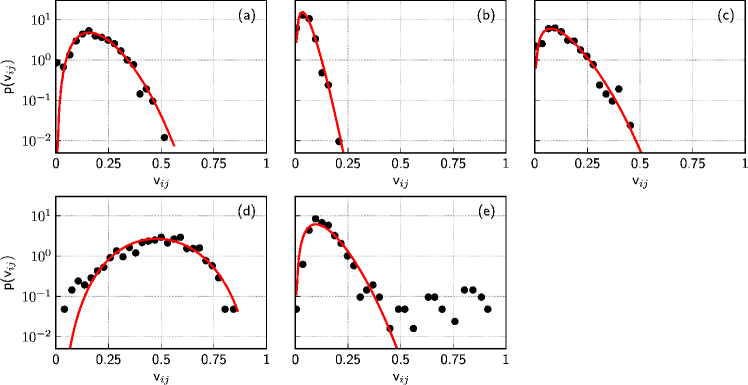
Figure 1: The vote share PDF of the most succesful parties during the 1992 election. The following parties were considered: SK (a), LSDP (b), LKDP (c), LDDP (d) and O (e). The empirical values are shown as black circles, while theoretical fits using the Beta distribution are shown as solid curves. The values of the Beta distribution parameters are given in Table 1.

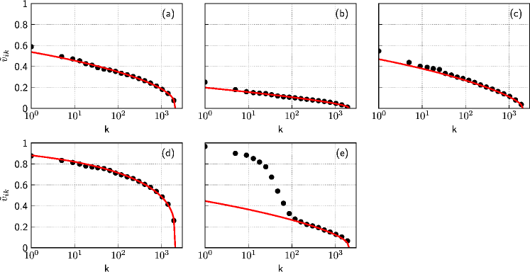
Figure 2: The rank-size distribution of the most succesful parties during the 1992 election. The following parties were considered: SK (a), LSDP (b), LKDP (c), LDDP (d) and O (e). The empirical values are shown as black circles, while theoretical fits using the Beta distribution are shown as solid curves. The values of the Beta distribution parameters are given in Table 1.

Table 1: Parameters of the Beta distribution, $\alpha$ and $\beta$, used to fit the data in Figs. 1 and 2 as well as wellness of fit for the PDFs, $R_{PDF}^{2}$, and the rank-size distributions, $R_{RS}^{2}$.

Party	$\alpha$	$\beta$	$R_{PDF}^{2}$	$R_{RS}^{2}$
SK	$3.9$	$16.6$	$0.956$	$0.994$
LSDP	$2.7$	$51$	$0.935$	$0.953$
LKDP	$2.2$	$16$	$0.926$	$0.995$
LDDP	$5.7$	$6.1$	$0.907$	$0.998$
O	$3$	$19.4$	$0.895$	$0.854$

In Fig. 3 we confirm this intuition by splitting the LLS party away from the “Other” party. After the split the rank-size distribution of the “Other” party is well approximated by the Beta distribution with parameters $\alpha=4.9$, $\beta=35.4$ ($R_{RS}^{2}=0.992$). To provide a good fit for the LLS rank-size distribution we assume that underlying data is distributed according to a mixture of the two Beta distributions: one ($95\%$ of points) with parameters $\alpha_{1}=0.08$, $\beta_{1}=10$ and the other ($5\%$ of points) with parameters $\alpha_{2}=1.22$, $\beta_{2}=1.37$.

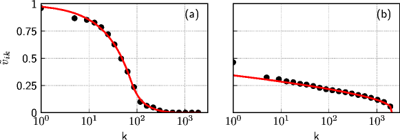
Figure 3: The rank-size distributions of the LLS (a) party and the other parties in the O party (b). The empirical values are shown as black circles, while solid curves provide fits by assuming that: $v_{ij}\sim 0.95\cdot\mathcal{B}e(0.08,10)+0.05\mathcal{\cdot B}e(1.22,1.37)$ ($R_{RS}^{2}=0.997$; (a)), $v_{ij}\sim\mathcal{B}e(4.9,35.4)$ ($R_{RS}^{2}=0.992$; (b)).

The parties’ vote share rank-size distributions were previously considered in [57]. Unlike in this paper, Fenner and others assumed that the parties’ vote share is distributed according Weibull distribution, they have obtained rather good fits for the UK election data. Yet fits obtained here, assuming Beta distribution, are also rather good. We believe that Beta distribution is superior for this purpose from the theoretical point of view. Namely, Beta distribution has reasonable support, probabilities are defined for $v\in\left[0;1\right]$, while Weibull distribution needs to be arbitrary truncated, as probabilities are defined for $v\in\left[0;+\infty\right)$. Interestingly Fenner and others also use a mixture distribution (of two Weibull distributions) to fit the UK election data. Similar observations were also made when studying Brazilian presidential election data [62]. In [63] it was noted that multiple different distributions, Weibull, log-normal and normal, provide good fits for the distribution of religions’ adherents. To discriminate between the possibilities a deeper theoretical insight is needed.

2.2 The parliamentary election of 2008

The parliamentary election of 2008 was held in $2034$ polling stations, yet we have only $1983$ points in the data set as the data from $51$ polling stations is missing. In this election a slightly smaller number of parties had participated ($16$), but now $7$ of them were able to obtain more than $5\%$ of popular vote. For the sake of simplicity we will use the following abbreviations for them: LSDP – “Lietuvos socialdemokratų partija” (formed by LSDP and LDDP, which participated in the 1992 election), TS-LKD – “Tėvynės sąjunga – Lietuvos krikščionys demokratai” (could be considered to be a successor of the SK and LKDP, which participated in the 1992 election), TPP – “Tautos prisikėlimo partija”, DP – “Koalicija Darbo partija + jaunimas”, LRLS – “Lietuvos Respublikos liberalų sąjūdis”, TT – “Partija Tvarka ir teisingumas”, LiCS – “Liberalų ir centro sąjunga”. As previously all other parties ($9$ of them) were combined to form the “Other” party (abbr. O). We have considered the votes cast for the combined “Other” party alongside the votes cast for the $7$ main parties.

As is evident from Figs. 4 and 5 in the 2008 election the vote share distributions of the most of the parties are well fitted by a mixture of two Beta distributions. Although now there is no clear-cut explanation for this phenomenon, we would like to conjecture that this observation indicates that other spatial segregations (e.g., by income) of voters in Lithuania have started to play an important role. Namely, most of the parties could now be identified with specific socio-economic classes, e.g., some party starts favoring higher income voters (gaining the support in cities), consequently losing the support of poorer voters (losing the support in rural areas).

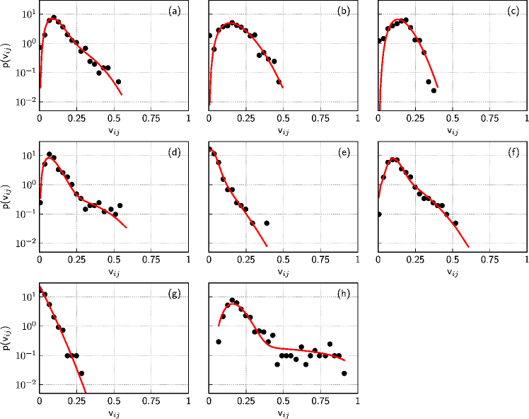
Figure 4: The vote share PDFs of the most succesful parties during the 2008 election. The following parties were considered: LSDP (a), TS-LKD (b), TPP (c), DP (d), LRLS (e), TT (f), LiCS (g) and O (h). The empirical values are shown as black circles, while theoretical fits using a mixture of Beta distributions are shown as solid curves (the values of the parameters are given in Table 2).

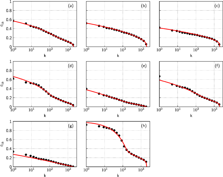
Figure 5: The rank-size distributions of the most succesful parties during the 2008 election. The following parties were considered: LSDP (a), TS-LKD (b), TPP (c), DP (d), LRLS (e), TT (f), LiCS (g) and O (h). The empirical values are shown as black circles, while theoretical fits using a mixture of Beta distributions are shown as solid curves (the values of the parameters are given in Table 2).

Table 2: The parameters of a mixture of Beta distributions, here $c$ is a weight of $\mathcal{B}e\left(\alpha_{2},\beta_{2}\right)$, used to fit the data in Figs. 4 and 5 as well as wellness of fit for the PDFs, $R_{PDF}^{2}$, and the rank-size distributions, $R_{RS}^{2}$.

Party	$\alpha_{1}$	$\beta_{1}$	$c$	$\alpha_{2}$	$\beta_{2}$	$R_{PDF}^{2}$	$R_{RS}^{2}$
LSDP	$3.9$	$31.7$	$0.15$	$4.3$	$12.9$	$0.968$	$0.999$
TS-LKD	$3.7$	$16.8$	$0$	–	–	$0.915$	$0.999$
TPP	$5.1$	$27.8$	$0$	–	–	$0.884$	$0.992$
DP	$3$	$30.3$	$0.09$	$3.2$	$7.7$	$0.942$	$0.992$
LRLS	$2.7$	$67.9$	$0.54$	$0.6$	$12.6$	$0.986$	$0.994$
TT	$7.6$	$59.5$	$0.42$	$1.8$	$9.4$	$0.987$	$0.992$
LiCS	$0.98$	$23.5$	$0$	–	–	$0.955$	$0.993$
O	$6.6$	$30.4$	$0.15$	$1.2$	$1.6$	$0.944$	$0.995$

2.3 The parliamentary election of 2012

The parliamentary election of 2012 was held in $2017$ polling stations (thus we have $2017$ data points). $18$ parties had participated in the election, while $7$ of them were able to obtain more than $5\%$ of popular vote. For the sake of simplicity we will use the following abbreviations for them: LRLS – “Lietuvos Respublikos liberalų sąjūdis”, DP – “Darbo partija”, TS-LKD – “Tėvynės sąjunga – Lietuvos krikščionys demokratai”, DK – “Drąsos kelias politinė partija”, LLRA – “Lietuvos lenkų rinkimų akcija”, LSDP – “Lietuvos socialdemokratų partija”, TT – “Partija Tvarka ir teisingumas”. Matching abbreviations indicate the same (or mostly the same) parties as in 2008 election. Once again the less-succesful parties were combined to form the “Other” party (abbr. O). The votes cast for the combined “Other” party were analyzed alongside the votes cast for the $7$ main parties.

Once again, as well as in the 2008 parliamentary election data set, it is evident that the vote share distributions of the most of the parties in the 2012 parliamentary are also well described by a mixture of two Beta distributions (see Figs. 6 and 7).

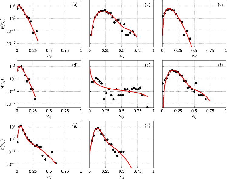
Figure 6: The vote share PDFs of the most succesful parties during the 2012 election. The following parties were considered: LRLS (a), DP (b), TS-LKD (c), DK (d), LLRA (e), LSDP (f), TT (g) and O (h). The empirical values are shown as black circles, while theoretical fits using a mixture of Beta distributions are shown as solid curves (the values of parameters are given in Table 3).

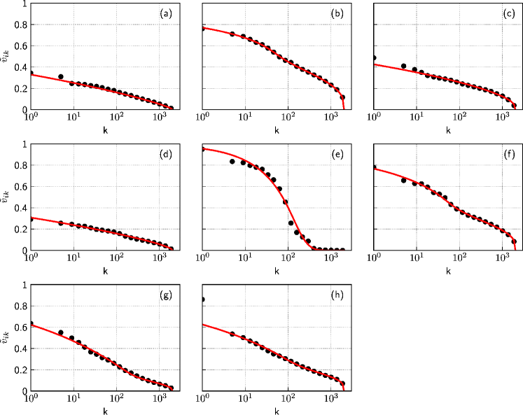
Figure 7: The rank-size distributions of the most succesful parties during the 2012 election. The following parties were considered: LRLS (a), DP (b), TS-LKD (c), DK (d), LLRA (e), LSDP (f), TT (g) and O (h). The empirical values are shown as black circles, while theoretical fits using a mixture of Beta distributions are shown as solid curves (the values of parameters are given in Table 3).

Table 3: The parameters of a mixture of Beta distributions, here $c$ is a weight of $\mathcal{B}e\left(\alpha_{2},\beta_{2}\right)$, used to fit the data in Figs. 6 and 7 as well as wellness of fit for the PDFs, $R_{PDF}^{2}$, and the rank-size distributions, $R_{RS}^{2}$.

Party	$\alpha_{1}$	$\beta_{1}$	$c$	$\alpha_{2}$	$\beta_{2}$	$R_{PDF}^{2}$	$R_{RS}^{2}$
LRLS	$1.5$	$22$	$0$	–	–	$0.969$	$0.994$
DP	$4.5$	$14.5$	$0.03$	$15.3$	$11.1$	$0.973$	$0.999$
TS-LKD	$3.4$	$22$	$0$	–	–	$0.938$	$0.982$
DK	$1.9$	$26$	$0$	–	–	$0.946$	$0.994$
LLRA	$0.06$	$1.9$	$0.05$	$2.1$	$1.9$	$0.857$	$0.990$
LSDP	$5$	$21.4$	$0.05$	$5.5$	$6.6$	$0.948$	$0.997$
TT	$4.6$	$62$	$0.29$	$1.1$	$6.7$	$0.963$	$0.995$
O	$7$	$45.8$	$0.23$	$2$	$8$	$0.966$	$0.970$

3 A multi-state agent-based model of the voting behavior

In this section we propose a simple multi-state agent-based model, which is to describes the voting behavior within a small non-specific geographic region covered by a single polling station. Unlike in some previous approaches [13, 14, 15, 16, 17, 18, 19, 20], our aim is not to incorporate complex ideas from psychology, but to reproduce the empirical parties’ vote share distribution. It is known that an agent-based herding model proposed by Alan Kirman, in [41], reproduces Beta distribution. So let us start by introducing Kirman’s herding model.

Originally in [41] Kirman noted that biologists and economists observe similar behavioral patterns. Apparently both ants and people show interest in things which are more popular among their peers regardless of their objective properties [64, 65, 66, 67, 68]. In [41] a simple two-state model was proposed to explain these observations. In the contemporary interpretations of the Kirman’s model the following mathematical form of the one step transition probabilities is used (see [42, 43, 44, 45]):

$$P(X\rightarrow X+1) = \left(N-X\right)\left(\sigma_{1}+hX\right)\Delta t,$$ (4)

$$P\left(X\rightarrow X-1\right) = X\left[\sigma_{2}+h\left(N-X\right)\right]\Delta t,$$ (5)

here $N$ is a total number of agents acting in the system, $X$ is a total number of agents occupying the first state (consequently there are $N-X$ agents occupying the second state), $\sigma_{i}$ are the perceived attractiveness parameters (may differ for different states), $h$ is a recruitment efficiency parameter and $\Delta t$ is a relatively short time step.

Let us now show that the two state model produces Beta distribution. This can be done by using birth–death process formalism, which is well described in [69]. The dynamics of $x=\frac{X}{N}$ (let $N$ be large) can be alternatively described by the following master equation:

$$\frac{\Delta\omega(x,t)}{\Delta t}=N^{2}\left\{({\bf E}-1)[\pi^{-}(x)\omega(x,t)]+({\bf E^{-1}}-1)[\pi^{+}(x)\omega(x,t)]\right\},$$ (6)

here $\omega(x,t)$ is time–dependent distribution, $\pi^{\pm}(x)$ are the transition rates per unit of time (defined as $\pi^{\pm}(x)=\frac{p(X\rightarrow X\pm 1)}{N^{2}h\Delta t}$), $\mathbf{E}$ and $\mathbf{E}^{-1}$ are the one step increment and decrement operators. Let us expand these operators in Taylor series up to the second order term:

$${\bf E}[f(x)] = f(x+\Delta x)\approx f(x)+\Delta x\frac{\operatorname{d}}{\operatorname{d}x}f(x)+\frac{\Delta x^{2}}{2}\frac{\operatorname{d}^{2}}{\operatorname{d}x^{2}}f(x),$$ (7)

$${\bf E^{-1}}[f(x)] = f(x-\Delta x)\approx f(x)-\Delta x\frac{\operatorname{d}}{\operatorname{d}x}f(x)+\frac{\Delta x^{2}}{2}\frac{\operatorname{d}^{2}}{\operatorname{d}x^{2}}f(x),$$ (8)

here $\Delta x=1/N$. Putting these Taylor expansions back into the master equation as well as taking small time step limit, yields the following Fokker–Planck equation:

$$\frac{\partial}{\partial t}\omega(x,t) =-\frac{\partial}{\partial x}[A(x)\omega(x,t)]+\frac{1}{2}\frac{\partial^{2}}{\partial x^{2}}[B(x)\omega(x,t)],$$ (9)

$$A(x) =N\left[\pi^{+}(x)-\pi^{-}(x)\right]=\varepsilon_{1}\left(1-x\right)-\varepsilon_{2}x,$$ (10)

$$B(x) =\pi^{+}(x)+\pi^{-}(x)=2x(1-x)+\mathcal{O}\left(N^{-1}\right),$$ (11)

where $\varepsilon_{i}=\sigma_{i}/h$. Steady–state distribution of this Fokker–Planck equation can be obtained by solving:

$$A(x)\omega_{st}(x)-\frac{1}{2}\frac{\partial}{\partial x}[B(x)\omega_{st}(x)]=0.$$ (12)

In general case the solution of this ordinary differential equation is given by:

$$\omega_{st}(x)=\frac{C_{0}}{B(x)}\exp\left[2\int^{x}\frac{A(u)}{B(u)}\operatorname{d}u\right],$$ (13)

where $C_{0}$ is normalization constant. In our specific case we obtain a PDF for the Beta distribution, $\mathcal{B}e\left(\varepsilon_{1},\varepsilon_{2}\right)$,

$$\omega_{st}(x)=\frac{C_{0}}{2}x^{\varepsilon_{1}-1}\left(1-x\right)^{\varepsilon_{2}-1}.$$ (14)

As in the typical parliamentary election there are more than two competitors, we need to generalize the model to incorporate more than two states. From the conservation of the total number of agents $N$, we have:

$$P\left(X_{i}\rightarrow X_{i}\pm 1\right)=\sum_{j\neq i}P\left(X_{i}\rightarrow X_{i}\pm 1,X_{j}\rightarrow X_{j}\mp 1\right).$$ (15)

Assuming that the right hand side probabilities have the same form as Eqs. (4) and (5), we obtain:

$$P(X_{i}\rightarrow X_{i}+1) = \sum_{j\neq i}X_{j}\left(\sigma_{ji}+h_{ji}X_{i}\right)\Delta t,$$ (16)

$$P\left(X_{i}\rightarrow X_{i}-1\right) = X_{i}\sum_{j\neq i}\left[\sigma_{ij}+h_{ij}X_{j}\right]\Delta t,$$ (17)

These one step transition probabilities for $X_{i}$ depend not only on $X_{i}$ (as in the two-state model), but also on all the other $X_{j}$ (here $j\neq i$). To circumvent this potentially cumbersome dependence one needs to assume that $\sigma_{ij}=\sigma_{j}$ and $h_{ij}=h$ (where $j\neq i$). The first assumption, $\sigma_{ij}=\sigma_{j}$, means that the perceived attractiveness of any party does not depend on who is attracted to it. While the second assumption, $h_{ij}=h$, means that the recruitment mechanism is uniform (symmetric and independent of interacting agents). Note that these assumptions contrast with the assumptions underlying the bounded confidence model [15, 16]. Yet these assumptions are needed to ensure that $x_{i}=\frac{X_{i}}{N}$ is distributed according to the Beta distribution. After making these assumptions we can further simplify the one step transition probabilities:

$$P\left(X_{i}\rightarrow X_{i}+1\right) = \left(N-X_{i}\right)\left(\sigma_{i}+hX_{i}\right)\Delta t,$$ (18)

$$P\left(X_{i}\rightarrow X_{i}-1\right) = X_{i}\left(\sigma_{-i}+h\left[N-X_{i}\right]\right)\Delta t,$$ (19)

here $\sigma_{-i}=\sum_{j\neq i}\sigma_{j}$ is the total attractiveness of all of the competitors of the party $i$. By the analogy with the two state model it should be evident that

$$x_{i}\sim\mathcal{B}e\left(\varepsilon_{i},\varepsilon_{-i}\right).$$ (20)

Unlike the two-state model, it seems impossible to provide a useful general aggregated macroscopic description, using the Fokker-Planck equation or a set of stochastic differential equations, of the generalized $M$-state model. In [70] a three-state model was considered and given an aggregated macroscopic description, by a system of two stochastic differential equations, yet it was possible only under specific conditions.

The one step transition probabilities, while describe agent’s behavior, are still aggregate description of individual agent level dynamics. So some discussion on what do the Eqs. (18) and (19) represent is relevant. Selecting one random agent, per time step, and setting his switching probability to $\varepsilon_{-i}\Delta t_{s}$ gives us idiosyncratic behavior term, $X_{i}\varepsilon_{-i}\Delta t_{s}$. While selecting another random agent and, if the both agents vote for the different parties, allowing the first agent to copy the second agent’s voting preference gives us the recruitment term, $X_{i}(N-X_{i})\Delta t_{s}$. This description of agent level dynamics could be further generalized to allow the model to be run on the randomly generated networks [71, 72]. This agent-based algorithm might be seen to be a special case of the well known Voter model [49, 50, 51, 25, 53, 54].

4 The modeling of the parliamentary election

Now let us apply the proposed model to reproduce the empirical vote share PDFs and rank-size distributions, which were observed during the 1992 parliamentary election. Here we consider only the simplest case by ignoring the “Other” party and in this way removing distortions caused by the ethnic segregation (see the discussion in Section 2.1). We do not consider the segregated data, the full data of the 1992 parliamentary election or the data of the 2008 and 2012 parliamentary elections, as to account for the vote segregation a more sophisticated approach is needed. Namely, in order to account for the full complexity of the empirical data additional information, such as the spatial polling data or the socio-demographic data, would be needed. Although, in general, one could try to infer the correct partition of the polling stations, where the vote share distribution of each partion would be modelled using the proposed model using the same parameter set.

In Figs. 8 and 9 we compare the vote share PDFs and the rank-size distributions numerically generated by the proposed model, Eqs. (18) and (19), and the respective empirical vote share distributions of the 1992 parliamentary election. Yet we cannot use the previously empirically estimated Beta distribution parameters, by assuming $\alpha_{i}=\varepsilon_{i}$ and $\beta_{i}=\varepsilon_{-i}$, as model parameters, because an important model implication, $\sum_{l\neq i}\alpha_{l}=\beta_{i}$, doesn’t hold for the empirical data. Yet one may obtain the parameter values by fitting the empirical data with the model implication in mind.

As you can see from Figs. 8 and 9 as well as Table 4 the proposed model excellently fits three of the four parties. While for the LSDP the fit is not as good as one might expect. Note that model overestimates the success of LSDP (the solid curve is above black circles for small $k$ in subfigure (d)) and underestimates the electoral support of LDDP (the solid curve is below black circles for small $k$ in subfigure (h)). Thus it is likely that the LSDP had small perceived chance to win the 1992 election (their aggregated vote share was near $5\%$), thus voters who would actually consider voting for the LSDP cast their votes for the other left-wing party, which had better perceived chance at winning the 1992 election (aggregated vote share of LDDP was above $40\%$).

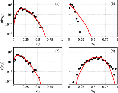
Figure 8: The vote share PDFs of the most succesful parties during the 1992 election fitted by the proposed model. Only the following parties were considered: SK (a), LSDP (b), LKDP (c) and LDDP (d). The empirical values are shown as black circles, while solid curves represent numerical results obtained from the proposed model, driven by Eqs. (18) and (19) (the same model run as in Fig. 9). The parameters of the model are given in Table 4.

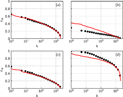
Figure 9: The the rank-size distributions of the most succesful parties during the 1992 election fitted by the proposed model. Only the following parties were considered: SK (a), LSDP (b), LKDP (c) and LDDP (d). The empirical values are shown as black circles, while solid curves represent numerical results obtained from the proposed model, driven by Eqs. (18) and (19) (the same model run as in Fig. 8). The parameters of the model are given in Table 4.

Table 4: The parameters of the proposed model used to reproduce the vote share PDFs and the rank-size distributions of the 1992 election as well as wellness of fit for the respective distributions.

Party	$\varepsilon_{i}$	$R_{PDF}^{2}$	$R_{RS}^{2}$
SK	$3.52$	$0.951$	$0.997$
LSDP	$1.13$	$0.705$	$0.881$
LKDP	$2.27$	$0.952$	$0.998$
LDDP	$8.87$	$0.904$	$0.973$

We can check this intuition by violating the assumption that the perceived attractivenes should not depend on the current state of the agent (agent’s currently supported party), namely instead of $\varepsilon_{i}$ we now have $\varepsilon_{ji}$. Previously this assumption was needed to ensure that vote share is distributed according to the Beta distribution. Let us introduce a single exception, if $j$ corresponds to LSDP and $i$ corresponds to LDDP, then $\varepsilon_{ji}$ can be differ in value from $\varepsilon_{i}$. This gives us the following matrix of $\varepsilon_{ji}$ values (the numeric indices are assigned according to Table 4):

$$\boldsymbol{\varepsilon}=\left(\begin{array}[]{cccc}0&1.13&2.27&8.87\\ 3.52&0&2.27&22\\ 3.52&1.13&0&8.87\\ 3.52&1.13&2.27&0\end{array}\right).$$ (21)

Note that the diagonal elements of the matrix $\mathbf{\varepsilon}$ are set to zero, as it is not possible to switch to the state the agent is already in. As you can see in Figs. 10 and 11, the fit provided by the model has significantly improved for the LSDP by just by making this small change.

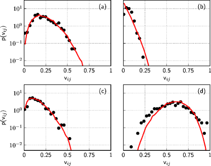
Figure 10: The vote share PDFs of the most popular parties during 1992 election fitted by the asymmetric model. Only the following parties were considered: SK (a), LSDP (b), LKDP (c) and LDDP (d). The empirical values are shown as black circles, while solid curves represent data numerically generated by the proposed model with attractiveness dependent on both current agent state and the perceived state. Model parameters are given by Eq. (21) (the same model run as in Fig. 11).

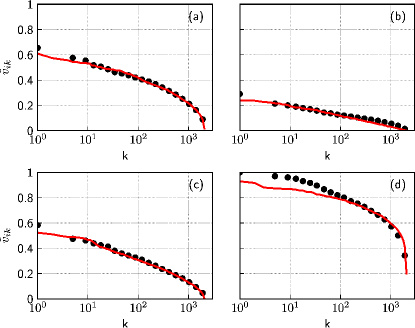
Figure 11: The rank-size distributions of the most popular parties during 1992 election fitted by the asymmetric model. Only the following parties were considered: SK (a), LSDP (b), LKDP (c) and LDDP (d). The empirical values are shown as black circles, while solid curves represent data numerically generated by the proposed model with attractiveness dependent on both current agent state and the perceived state. Model parameters are given by Eq. (21) (the same model run as in Fig. 10).

5 Conclusions

In this paper we have considered the parties’ vote share PDFs and the rank-size distributions observed during the Lithuanian parliamentary elections. Namely, we have considered the 1992, 2008 and 2012 parliamentary elections’ data sets. We have determined that the empirical vote share PDFs and the rank-size distributions are rather well fitted by assuming that the underlying distribution is the Beta distribution or a mixture of two Beta distributions. Reviewing literature we have found that [63, 62, 57, 54] have reported somewhat similar results. In [62, 57] it was reported that the empirical data is rather well fitted by a mixture of Weibull distributions. In [63] it was noted that multiple different distributions, Weibull, log-normal and normal, provide good fits for the distribution of religions’ adherents. We argue that the Beta distribution is more suitable as it has correct support (probabilities are defined for $v\in[0;1]$; although the other distributions could be arbitrary truncated) and it arises from a simple easily tractable agent-based model. From our empirical analysis it follows that the mixture of Beta distributions is needed to fit the data if there is underlying spatial segregation of the electorate. In [54] it is also reported that the empirical data is rather well fitted by Beta distribution, which arises from a noisy Voter model. Yet [54] did not observe the vote share segregation pattern.

Having in mind the stark difference between the psychologically motivated models, such as bounded confidence model [15, 16], we would like to point out that the observed statistical patterns as well as the applicability of the model could arise due to numerous unrelated reasons. One of the alternative possibilities would be the people mobility patterns. In the proposed model a single agent switching from supporting one party to supporting another party, could also represent one agent moving away from the modeled geographic location, due to social or economic reasons, and another agent, holding different political views, moving in. A similar idea was raised in [53].

In the nearest future we will consider spatial modeling of the Lithuanian parliamentary elections. Another possible approach, with forecasting possibility, could be considering a temporal regression model for the attractiveness parameters of the proposed model, $\varepsilon_{i}$, as well as the estimation of the agent interaction rates, $h$.

References

- [1] W. H. Riker and P. C. Ordeshook, “A theory of the calculus of voting,” The American Political Science Review, vol. 62, no. 1, pp. 25–42, 1968.
- [2] J. A. Ferejohn and M. P. Fiorina, “The paradox of not voting: A decision theoretic analysis,” American Political Science Review, vol. 68, no. 2, pp. 525–536, 1974.
- [3] C. J. Uhlaner, “Rational turnout: The neglected role of groups,” American Journal of Political Science, vol. 33, no. 2, pp. 390–422, 1989.
- [4] H. Hotelling, “Stability in competition,” The Economic Journal, vol. 39, no. 153, pp. 41–57, 1929.
- [5] A. Downs, “An economic theory of political action in a democracy,” Journal of Political Economy, vol. 65, no. 2, pp. 135–150, 1957.
- [6] D. Black, The Theory of Committees and Elections. Springer, 1958.
- [7] C. R. Plott, “A notion of equilibrium and its possibility under majority rule,” The American Economic Review, vol. 57, no. 4, pp. 787–806, 1967.
- [8] R. D. McKelvey, “Intransitivities in multidimensional voting models and some implications for agenda control,” Journal of Economic Theory, vol. 12, no. 3, pp. 472–482, 1976.
- [9] S. Ansolabehere and J. M. Snyder, “Valence politics and equilibrium in spatial election models,” Public Choice, vol. 103, no. 3/4, pp. 327–336, 2000.
- [10] W. B. Arthur, “Inductive reasoning and bounded rationality,” American Economic Review, vol. 84, pp. 406–411, 1994.
- [11] G. Akerlof and J. Shiller, Animal Spirits: How Human Psychology Drives the Economy, and Why It Matters for Global Capitalism. Princeton University Press, 2009.
- [12] D. Helbing and A. Kirman, “Rethinking economics using complexity theory.”
- [13] A. Nowak, J. Szamrej, and B. Latane, “From private attitude to public opinion: A dynamic theory of social impact,” Psychological Review, vol. 97, no. 3, pp. 362–376, 1990.
- [14] R. Axelrod, “The dissemination of culture a model with local convergence and global polarization,” Journal of Conflict Resolution, vol. 41, no. 2, pp. 203–226, 1997.
- [15] R. Hegselmann and U. Krause, “Opinion dynamics and bounded confidence: models, analysis and simulation,” Journal of Artificial Societies and Social Simulation, vol. 5, no. 3, p. 2, 2002.
- [16] G. Deffuant, “Comparing extremism propagation patterns in continuous opinion models,” Journal of Artificial Societies and Social Simulation, vol. 9, no. 3, p. 8, 2006.
- [17] P. Sobkowicz, “Discrete model of opinion changes using knowledge and emotions as control variables,” PLoS ONE, vol. 7, no. 9, p. e44489, 2012.
- [18] D. G. Lilleker, Modelling Political Cognition. London: Palgrave Macmillan UK, 2014, pp. 198–205.
- [19] P. Sobkowicz, “Quantitative agent based model of opinion dynamics: Polish elections of 2015,” PLoS ONE, vol. 11, no. 5, p. e0155098, 2016.
- [20] P. Duggins, “A psychologically-motivated model of opinion change with applications to american politics,” Journal of Artificial Societies and Social Simulation, vol. 20, no. 1, p. 13, 2017.
- [21] P. Ball, “The physical modelling of society: A historical perspective,” Physica A, vol. 314, pp. 1–14, 2002.
- [22] S. Galam, “Majority rule, hierarchical structures, and democratic totalitarianism: A statistical approach,” Journal of Mathematical Psychology, vol. 30, no. 4, pp. 426 – 434, 1986.
- [23] R. N. Mantegna and H. E. Stanley, Introduction to Econophysics: Correlations and Complexity in Finance. Cambridge University Press, 2000.
- [24] B. K. Chakrabarti, A. Chakraborti, and A. Chatterjee, Econophysics and Sociophysics - Trends and Perspectives. Wiley, 2006.
- [25] C. Castellano, S. Fortunato, and V. Loreto, “Statistical physics of social dynamics,” Reviews of Modern Physics, vol. 81, pp. 591–646, 2009.
- [26] D. Stauffer, “A biased review of sociophysics,” Journal of Statistical Physics, 2013.
- [27] F. Abergel, H. Aoyama, B. Chakrabarti, A. Chakraborti, N. Deo, D. Raina, and I. Vodenska, Eds., Econophysics and Sociophysics: Recent Progress and Future Directions. Springer, 2017.
- [28] K. Sznajd-Weron, “Sznajd model and its applications,” Acta Physica Polonica B, vol. 36, no. 8, pp. 2537–2548, 2005.
- [29] S. Galam, “Sociophysics: A review of galam models,” International Journal of Modern Physics C, vol. 19, no. 03, p. 409, 2008.
- [30] P. Nyczka and K. Sznajd-Weron, “Anticonformity or independence?—insights from statistical physics,” Journal of Statistical Physics, vol. 151, no. 1, pp. 174–202, 2013.
- [31] S. Fortunato and C. Castellano, “Scaling and universality in proportional elections,” Physical Review Letters, vol. 99, p. 138701, 2007.
- [32] C. A. Andresen, H. F. Hansen, A. Hansen, G. L. Vasconcelos, and J. S. Andrade Jr., “Correlations between political party size and voter memory: Statistical analysis of opinion polls,” International Journal of Modern Physics C, vol. 19, p. 1647, 2008.
- [33] C. Borghesi and J.-P. Bouchaud, “Spatial correlations in vote statistics: a diffusive field model for decision-making,” European Physical Journal B, vol. 75, no. 3, pp. 395–404, 2010.
- [34] M. C. Mantovani, H. V. Ribeiro, M. V. Moro, S. Picoli Jr., and R. S. Mendes, “Scaling laws and universality in the choice of election candidates,” EPL, vol. 96, no. 4, p. 48001, 2011.
- [35] C. Borghesi, J.-C. Raynal, and J. P. Bouchaud, “Election turnout statistics in many countries: similarities, differences, and a diffusive field model for decision-making,” PLoS ONE, vol. 7, p. e36289, 2012.
- [36] A. Krupavicius, “The lithuanian parliamentary elections of 1996,” Electoral Studies, vol. 16, no. 4, pp. 541 – 549, 1997.
- [37] M. Degutis, “How lithuanian voters decide: Reasons behind the party choice,” Lithuanian Political Science Yearbook, pp. 69–111, 2000.
- [38] M. Kreuzer and V. Pettai, “Patterns of political instability: Affiliation patterns of politicians and voters in post-communist estonia, latvia, and lithuania,” Studies in Comparative International Development, vol. 38, pp. 76–98, 2003.
- [39] M. Jurkynas, “Emerging cleavages in new democracies: The case of lithuania,” Journal of Baltic Studies, vol. 35, no. 3, pp. 278–296, 2004.
- [40] A. Ramonaite, The Development of the Lithuanian Party System: From Stability to Perturbation. Routledge, 2006, pp. 69–88.
- [41] A. P. Kirman, “Ants, rationality and recruitment,” Quarterly Journal of Economics, vol. 108, pp. 137–156, 1993.
- [42] S. Alfarano, T. Lux, and F. Wagner, “Estimation of agent-based models: The case of an asymmetric herding model,” Computational Economics, vol. 26, no. 1, pp. 19–49, 2005.
- [43] ——, “Time variation of higher moments in a financial market with heterogeneous agents: An analytical approach,” Journal of Economic Dynamics and Control, vol. 32, pp. 101–136, 2008.
- [44] V. Alfi, M. Cristelli, L. Pietronero, and A. Zaccaria, “Minimal agent based model for financial markets i: Origin and self-organization of stylized facts,” European Physics Journal B, vol. 67, no. 3, pp. 385–397, 2009.
- [45] A. Kononovicius and V. Gontis, “Agent based reasoning for the non-linear stochastic models of long-range memory,” Physica A, vol. 391, no. 4, pp. 1309–1314, 2012.
- [46] S. Alfarano, M. Milakovic, and M. Raddant, “A note on institutional hierarchy and volatility in financial markets,” The European Journal of Finance, vol. 19, no. 6, pp. 449–465, 2013.
- [47] V. Gontis and A. Kononovicius, “Consentaneous agent-based and stochastic model of the financial markets,” PLoS ONE, vol. 9, no. 7, p. e102201, 2014.
- [48] V. Gontis, S. Havlin, A. Kononovicius, B. Podobnik, and H. Stanley, “Stochastic model of financial markets reproducing scaling and memory in volatility return intervals,” Physica A, vol. 462, pp. 1091–1102, 2016.
- [49] P. Clifford and A. Sudbury, “A model for spatial conflict,” Biometrika, vol. 60, pp. 581 – 588, 1973.
- [50] T. Liggett, Stochastic Interacting Systems: Contact, Voter, and Exclusion Processes. Springer, 1999.
- [51] S. Galam, B. Chopard, and M. Droz, “Killer geometries in competing species dynamics,” Physica A, vol. 314, pp. 256 – 263, 2002.
- [52] C. Castellano, D. Vilone, and A. Vespignani, “Incomplete ordering of the voter model on small-world networks,” EPL, vol. 63, no. 1, p. 153, 2003.
- [53] J. Fernandez-Gracia, K. Suchecki, J. J. Ramasco, M. San Miguel, and V. M. Eguiluz, “Is the voter model a model for voters?” Physical Review Letters, vol. 112, p. 158701, 2014.
- [54] F. Sano, M. Hisakado, and S. Mori, “Mean field voter model of election to the house of representatives in japan,” 2016.
- [55] M. Jastramskis, “Forecasting the results of seimas elections: model of government parties’ votes,” Parlamento studijos, vol. 11, 2011.
- [56] S. Galam, “The invisible hand and the rational agent are behind bubbles and crashes,” Chaos, Solitons and Fractals, vol. 88, pp. 209 – 217, 2016.
- [57] T. Fenner, M. Levene, and L. G., “A multiplicative process for generating the rank-order distribution of uk election results,” Quality & Quantity, pp. 1–11, 2017.
- [58] G. K. Zipf, Human Behavior and the Principle of Least Effort. Addison-Wesley, 1949.
- [59] D. Sornette, L. Knopoff, Y. Y. Kagan, and C. Vanneste, “Rank-ordering statistics of extreme events: Application to the distribution of large earthquakes,” Journal of Geophysical Research, vol. 101, no. B6, pp. 13 883–13 893, 1996.
- [60] X. Gabaix, “Zipf’s law for cities: An explanation,” The Quarterly Journal of Economics, vol. 114, no. 3, p. 739, 1999.
- [61] J. Shao, P. C. Ivanov, B. Urosevic, H. E. Stanley, and B. Podobnik, “Zipf rank approach and cross-country convergence of incomes,” EPL, vol. 94, p. 48001, 2011.
- [62] R. F. d. Paz, R. S. Ehlers, and J. L. Bazan, A Weibull Mixture Model for the Votes of a Brazilian Political Party. Springer International Publishing, 2015, pp. 229–241.
- [63] M. Ausloos and F. Petroni, “Statistical dynamics of religions and adherents,” EPL, vol. 77, no. 3, p. 38002, 2007.
- [64] F. M. Bass, “A new product growth model for consumer durables,” Management Science, vol. 15, pp. 215–227, 1969.
- [65] J. M. Pasteels, J. L. Deneubourg, and S. Goss, “Self-organization mechanisms in ant societies (i): Trail recruitment to newly discovered food sources,” in From Individual to Collective Behaviour in Social Insects, J. M. Pasteels and J. L. Deneubourg, Eds. Basel: Birkhauser, 1987, pp. 155–175.
- [66] ——, “Self-organization mechanisms in ant societies (ii): Learning in foraging and division of labor,” in From Individual to Collective Behaviour in Social Insects, J. M. Pasteels and J. L. Deneubourg, Eds. Basel: Birkhauser, 1987, pp. 177–196.
- [67] G. S. Becker, “A note on restaurant pricing and other examples of social influence on price,” Journal of Political Economy, vol. 99, pp. 1109–1116, 1991.
- [68] A. Ishii, H. Arakaki, N. Matsuda, S. Umemura, T. Urushidani, N. Yamagata, and N. Yoshda, “The ’hit’ phenomenon: a mathematical model of human dynamics interactions as a stochastic process,” New Journal of Physics, vol. 14, p. 063018, 2012.
- [69] N. G. van Kampen, Stochastic process in Physics and Chemistry. Amsterdam: North Holland, 2007.
- [70] A. Kononovicius and V. Gontis, “Three state herding model of the financial markets,” EPL, vol. 101, p. 28001, 2013.
- [71] S. Alfarano and M. Milakovic, “Network structure and n-dependence in agent-based herding models,” Journal of Economic Dynamics and Control, vol. 33, no. 1, pp. 78–92, 2009.
- [72] A. Kononovicius and J. Ruseckas, “Continuous transition from the extensive to the non-extensive statistics in an agent-based herding model,” European Physics Journal B, vol. 87, no. 8, p. 169, 2014.