Multivariate Count Autoregression

Abstract

We are studying the problems of modeling and inference for multivariate count time series data with Poisson marginals. The focus is on linear and log-linear models. For studying the properties of such processes we develop a novel conceptual framework which is based on copulas. However, our approach does not impose the copula on a vector of counts; instead the joint distribution is determined by imposing a copula function on a vector of associated continuous random variables. This specific construction avoids conceptual difficulties resulting from the joint distribution of discrete random variables yet it keeps the properties of the Poisson process marginally. We employ Markov chain theory and the notion of weak dependence to study ergodicity and stationarity of the models we consider. We obtain easily verifiable conditions for both linear and log-linear models under both theoretical frameworks. Suitable estimating equations are suggested for estimating unknown model parameters. The large sample properties of the resulting estimators are studied in detail. The work concludes with some simulations and a real data example.

Keywords: autocorrelation, copula, ergodicity, generalized linear models, perturbation, prediction, stationarity, volatility.

1 Introduction

Modeling and inference of multivariate count time series is an important topic for research as such data can be observed in several applications; see Paul et al. (2008) for a medical application, Boudreault and Charpentier (2011) who study the number of earthquake occurrences, Pedeli and Karlis (2013b) for a financial application and more recently Ravishanker et al. (2015) for a marketing application. Some early work in this research direction can be found in Franke and Rao (1995) and Latour (1997). The interested reader is referred to the review paper by Karlis (2016), for further details.

The available literature shows that there exist three main approaches taken towards the problem of modeling and inference for multivariate count time series. The first approach is based on the theory of integer autoregressive (INAR) models and was initiated by Franke and Rao (1995) and Latour (1997). This work was further developed by Pedeli and Karlis (2013a, b) and a review of this methodology has been recently given by Karlis (2016). Estimation for these models is based on least squares methodology and likelihood based methods. However, even in the context of univariate INAR models, likelihood theory is quite cumbersome, especially for higher order models. Therefore, this class of models, which is adequate to describe some simple data structures, still poses challenges in terms of estimation (and prediction) especially when the model order is large.

The second class of models that have been proposed for the analysis of count time series models, is that of parameter driven models. Recall that a parameter driven model (according to the broad categorization introduced by Cox (1981)) is a model whose dynamics are driven by an unobserved process. In this case, state space models for multivariate count time series were studied by Jørgensen et al. (1996) and Jung et al. (2011) who suggested a factor model for the analysis of multivariate count time series; see also Ravishanker et al. (2014); Ravishanker et al. (2015), among others, for more recent contributions.

The aim of our contribution is to study models that fall within the class of observation driven models; that is models whose dynamics evolve according to past values of the process itself plus some noise. This is the case of the usual autoregressive models. In particular, observation driven models for count time series have been studied by Davis et al. (2000), Fokianos et al. (2009a), Fokianos and Tjøstheim (2011) Davis and Liu (2016), among others. There is a growing recent literature in the topic of modeling and inference for observation driven models for multivariate count time series; see Heinen and Rengifo (2007), Liu (2012), Andreassen (2013), Ahmad (2016) and Lee et al. (2017), for instance. These studies are mainly concerned with linear model specifications. Although the linear model is adequate for studying properties of the multivariate process, it may not always be a natural candidate for count data analysis. The log-linear model is more appropriate, in our view, for general modeling of count time series. Some desirable properties of log-linear models are the ease of including covariates, incorporation of positive/negative correlation and avoiding parameter boundary problems (see Fokianos and Tjøstheim (2011)). In fact, a log-linear model corresponds to the canonical link Poisson regression model for count data analysis (McCullagh and Nelder (1989)).

Besides modeling issues, another obstacle for the analysis of count time series is the choice of the joint count distribution. Indeed, there are numerous proposals available in the literature generalizing the univariate Poisson probability mass function (pmf); some of these are reviewed in the previous references. However, the pmf of a multivariate Poisson discrete random vector is usually of quite complicated functional form and therefore maximum likelihood based inference can be quite challenging (theoretically and numerically). Generally speaking, the choice of the joint distribution for multivariate count data is quite an interesting topic but in this work we have chosen to address this problem by suggesting a copula based construction. Instead of imposing a copula function on a vector of discrete random variables, we argue, based on Poisson process properties, that it can be introduced on a vector of continuous random variables. In this way, we avoid some technical difficulties and we propose a plausible data generating process which keeps intact the properties of the Poisson properties, marginally. Having resolved the problems of data generating process and given a model, we suggest suitable estimating functions to estimate the unknown parameters. The main goals of this work are summarized by the following:

1. Develop a conceptual framework for studying count time series with Poisson process marginally. As it was explained earlier, one of the problems posed in this setup, is the choice of the joint count distribution. We resolve this issue by imposing a copula structure for accommodating dependence, yet the properties of Poisson processes are kept marginally.

2. Give conditions for ergodicity and stationarity of both linear and log-linear models. The preferred methodologies are those of Markov chain theory (employing a perturbation approach) and theory of weak dependence. Although the linear model was treated by Liu (2012) in a parametric joint Poisson framework, we relax these conditions considerably when using the perturbation approach. For the log-linear model case, these conditions are new.

3. Furthermore, we suggest a class of estimating functions for inference. As it was discussed earlier, the specification of a joint distribution of a count vector poses several challenges. We overcome this obstacle by suggesting appropriate estimating functions which still deliver consistent and asymptotically normally distributed estimators.

As a final remark we discuss the challenges associated with the problem of showing stationarity and ergodicity of count time series. The main obstacle–see Neumann (2011) and Tjøstheim (2012, 2015)–is that the process itself consists of integer valued random variables; however the mean process takes values on the positive real line which creates difficulties in proving ergodicity of the observed process (see Andrews (1984) for a related situation). The study of theoretical properties of these models was initiated by the perturbation method suggested in Fokianos et al. (2009a) and was further developed in Neumann (2011) ($\beta$-mixing), (Doukhan et al., 2012b) (weak dependence approach, see Doukhan and Louhichi (1999)), Douc et al. (2013) (Markov chain theory without irreducibility assumptions) and Wang et al. (2014) (based on the theory of $e$-chains; see Meyn and Tweedie (1993)). We note that Doukhan et al. (2012a) study the relation between weak dependence coefficients defined in Doukhan and Louhichi (1999)) and the strong mixing coefficients (Rosenblatt (1956)) for the case of integer valued count time series. As it was mentioned before, we will be employing Markov chain theory (using the perturbation approach) and the notion of weak dependence for studying both linear and log-linear models. The end results obtained by either approach are identical when there is no feedback process in the model; however these results change when a hidden process is included in the model.

The paper is organized as follows: Section 2 discusses the basic modeling approach that we take towards modeling multivariate count time series. The copula structure which is imposed introduces dependence but without affecting the properties of the marginal Poisson processes. We will consider both a linear and a log-linear model. Section 3 gives the results about ergodic and stationary properties of the linear and log-linear models. Section 4 discusses Quasi Maximum Likelihood inference (QMLE) and shows that the resulting estimators are consistent and asymptotically normal. Section 5 presents a limited simulation study and a real data examples. The paper concludes with a discussion and an appendix which contains the proofs of main results and supplementary material.

2 Model Assumptions

In what follows we assume that $\{{\bf Y}_{t}=(Y_{i,t}),~{}i=1,\ldots,p,~{}t=1,2\ldots,\}$ denotes a $p$–dimensional count time series. Let $\{{\mbox{\boldmath$\bf\lambda$}}_{t}=(\lambda_{i,t}),~{}i=1,\ldots,p,t=1,2,\ldots\}$ be the corresponding $p$-dimensional intensity process and ${\cal F}_{t}^{\mbox{\boldmath$\bf Y$},\mbox{\boldmath$\bf\lambda$}}$ the $\sigma$–field generated by $\{\mbox{\boldmath$\bf Y$}_{0},\cdots,\mbox{\boldmath$\bf Y$}_{t},\mbox{\boldmath$\bf\lambda$}_{0}\}$ with ${\mbox{\boldmath$\bf\lambda$}}_{0}$ being a $p$-dimensional vector denoting the starting value of $\{\mbox{\boldmath$\bf\lambda$}_{t}\}$. With this notation, the intensity process is given by ${\mbox{\boldmath$\bf\lambda$}}_{t}=\mbox{E}[\mbox{\boldmath$\bf Y$}_{t}\mid{\cal F}_{t}^{\mbox{\boldmath$\bf Y$},\mbox{\boldmath$\bf\lambda$}}]$. We will be studying two autoregressive models for multivariate count time series analysis; the linear and log-linear models which are direct extensions of their univariate counterparts.

The linear model is defined by assuming that for each $i=1,2,\ldots,p$,

$$Y_{i,t}\mid{\cal F}_{t-1}^{\mbox{\boldmath$\bf Y$},\mbox{\boldmath$\bf\lambda$}}~{}~{}\mbox{is marginally}~{}~{}\mbox{Poisson}(\lambda_{i,t}),~{}~{}{\mbox{\boldmath$\bf\lambda$}}_{t}={\bf d}+{\bf A}{\mbox{\boldmath$\bf\lambda$}}_{t-1}+{\bf B}{\bf Y}_{t-1},$$ (1)

where ${\bf d}$ is a $p$-dimensional vector and ${\bf A}$, ${\bf B}$ are $p\times p$ unknown matrices. The elements of ${\bf d}$, ${\bf A}$ and ${\bf B}$ are assumed to be positive for ensuring positivity of $\lambda_{i,t}$. Model (1) generalizes naturally the linear autoregressive model discussed by Rydberg and Shephard (2000), Heinen (2003), Ferland et al. (2006) and Fokianos et al. (2009a), among others. The log-linear model that we consider is the multivariate analogue of the univariate log-linear model proposed by Fokianos and Tjøstheim (2011) (see also Woodard et al. (2011) and Douc et al. (2013)); more precisely assume that for each $i=1,2,\ldots,p$,

$$Y_{i,t}\mid{\cal F}_{t}^{\mbox{\boldmath$\bf Y$},\mbox{\boldmath$\bf\lambda$}}~{}~{}\mbox{is marginally}~{}~{}\mbox{Poisson}(\lambda_{i,t}),~{}~{}{\mbox{\boldmath$\bf\nu$}}_{t}={\bf d}+{\bf A}{\mbox{\boldmath$\bf\nu$}}_{t-1}+{\bf B}\log({\bf Y}_{t-1}+{\bf 1}_{p}),$$ (2)

where ${\mbox{\boldmath$\bf\nu$}}_{t}\equiv\log{\mbox{\boldmath$\bf\lambda$}}_{t}$ is defined componentwise (i.e. $\nu_{i,t}=\log\lambda_{i,t}$) and ${\bf 1}_{p}$ denotes the $p$–dimensional vector which consists of ones. In the case of (2), we do not impose any positivity constraints on the parameters ${\bf d}$, ${\bf A}$ and ${\bf B}$; this is an important argument favoring the log-linear model. We will examine aspects of both models. The log-linear model (2) is expected to be a better candidate for count data observed jointly with some other covariate time series or where negative correlation is observed.

A fundamental problem in the analysis of multivariate count data is the specification of joint distribution of the counts. There are numerous proposals made in the literature aiming on generalizing the univariate Poisson assumption to the multivariate case but the resulting joint distributions are quite complex for likelihood based inference. For instance, a possible construction can be based on independent Poisson random variables or on copulas and mixture models (see Johnson et al. (1997, Ch. 37), Joe (1997, Sec 7.2)). However, the resulting functional form of the joint pmf is complicated and therefore the log-likelihood function cannot be calculated analytically (or, sometimes, even approximated).

We propose a quite different approach. Consider the first equation of (1) (but the same discussion applies to (2) subject to minor modifications). It implies that each component $Y_{i,t}$ is marginally a Poisson process. But the joint distribution of the vector $\{{\bf Y}_{t}\}$ is not necessarily distributed as a multivariate Poisson random variable. Our general construction, as outlined below, allows for arbitrary dependence among the marginal Poisson components by utilizing fundamental properties of the Poisson process. We give a detailed account of the data generating process. Suppose that $\mbox{\boldmath$\bf\lambda$}_{0}=(\lambda_{1,0},\ldots,\lambda_{p,0})$ is some starting value. Then consider the following data generating mechanism:

1. Let ${\mbox{\boldmath$\bf U$}}_{l}=(U_{1,l},\ldots,U_{p,l})$ for $l=1,2,\ldots,K$, be a sample from a $p$-dimensional copula $C(u_{1},\ldots,u_{p})$. Then $U_{i,l}$, $l=1,2,\ldots,K$ follow marginally the uniform distribution on $(0,1)$, for $i=1,2,\ldots,p$.

2. Consider the transformation

   $$X_{i,l}=-\frac{\log U_{i,l}}{\lambda_{i,0}},~{}~{}~{}i=1,2,\ldots,p.$$

   Then, the marginal distribution of $X_{i,l}$, $l=1,2,\ldots,K$ is exponential with parameter $\lambda_{i,0}$, $i=1,2,\ldots,p$.

3. Define now (taking $K$ large enough)

   $$Y_{i,0}=\max_{1\leq k\leq K}\left\{\sum_{l=1}^{k}X_{i,l}\leq 1\right\},~{}~{}~{}i=1,2,\ldots,p.$$

   Then ${\bf Y}_{0}=(Y_{1,0},\ldots,Y_{p,0})$ is marginally a set of first values of a Poisson process with parameter $\mbox{\boldmath$\bf\lambda$}_{0}$.

4. Use model (1) (respectively (2)) to obtain $\mbox{\boldmath$\bf\lambda$}_{1}$.

5. Return back to step 1 to obtain ${\bf Y}_{1}$, and so on.

The aforementioned construction of the joint distribution of the counts imposes the dependence among the components of the vector process $\{{\bf Y}_{t}\}$ by taking advantage of a copula structure on the waiting times of the Poisson process. This can be extended to other marginal processes if they can be generated by continuous inter arrival times. Equivalently, the copula is imposed on the uniform random variables generating the exponential waiting times. Such an approach does not pose any problems on obtaining the joint distribution of the random vector $\{{\bf Y}_{t}\}$ which is composed of discrete valued random variables. The copula is defined uniquely for continuous multivariate random variables (compare with Heinen and Rengifo (2007) and for a lucid discussion about copula for discrete multivariate distributions, see Genest and Nešlehová (2007)). Hence, the first equation of model (1) can be restated as

$${\mbox{\boldmath$\bf Y$}}_{t}={\bf{N}}_{t}({\mbox{\boldmath$\bf\lambda$}}_{t}),~{}~{}~{}{\mbox{\boldmath$\bf\lambda$}}_{t}={\bf d}+{\bf A}{\mbox{\boldmath$\bf\lambda$}}_{t-1}+{\bf B}{\bf{Y}}_{t-1}$$ (3)

where $\{{\bf N}_{t}\}$ is a sequence of independent $p$-variate copula–Poisson processes which counts the number of events in $[0,\lambda_{1,t}]\times\ldots\times[0,\lambda_{p,t}]$. Along the lines of introducing (3) we also define the multivariate log–linear model (2) by

$${\mbox{\boldmath$\bf Y$}}_{t}={\bf{N}}_{t}({\mbox{\boldmath$\bf\nu$}}_{t}),~{}~{}~{}{\mbox{\boldmath$\bf\nu$}}_{t}={\bf d}+{\bf A}{\mbox{\boldmath$\bf\nu$}}_{t-1}+{\bf B}\log({\bf{Y}}_{t-1}+{\bf 1}_{p})$$ (4)

recalling that ${\mbox{\boldmath$\bf\nu$}}_{t}=\log{\mbox{\boldmath$\bf\lambda$}}_{t}$ is defined componentwise and ${\bf 1}_{p}$ denotes the $p$–dimensional vector which consists of ones. The process $\{{\bf N}_{t}\}$ denotes as before a sequence of independent $p$-variate copula–Poisson processes which counts the number of events in $[0,\exp(\nu_{1,t})]\times\ldots\times[0,\exp(\nu_{p,t})]$.

It is instructive to consider model (3) in more detail because its structure is closely related to the theory of GARCH models, Bollerslev (1986). Observe that each component of the vector-process $\{\mbox{\boldmath$\bf Y$}_{t}\}$ is distributed as a Poisson random variable. But the mean of a Poisson random variable equals its variance; therefore model (3) resembles some structure of multivariate GARCH model, see Lütkepohl (2005) and Francq and Zakoïan (2010). Consider $p=2$, for example. Then the second equation of (3) becomes

$$\lambda_{1,t} = d_{1}+a_{11}\lambda_{1,t-1}+a_{12}\lambda_{2,t-1}+b_{11}Y_{1,t-1}+b_{12}Y_{2,t-1},$$

$$\lambda_{2,t} = d_{2}+a_{21}\lambda_{1,t-1}+a_{22}\lambda_{2,t-1}+b_{21}Y_{1,t-1}+b_{22}Y_{2,t-1},$$

where $d_{i}$ is the $i$th element of $\bf d$ and $a_{ij}$ ($b_{ij}$, respectively) is the $(i,j)$th element of $\bf A$ ($\bf B$, respectively). We can give the following interpretation to model parameters. When $a_{12}=b_{12}=0$, then $\lambda_{1t}$ depends only on its own past. If this is not true, then the parameters denote the linear dependence of $\lambda_{1t}$ on $\lambda_{2,t-1}$ and $Y_{2,t-1}$ in the presence of $\lambda_{1,t-1}$ and $Y_{1,t-1}$. Similar results hold when $a_{21}=b_{21}=0$ and the previous discussion applies to the case of (4).

This section introduced the approach we take towards modeling multivariate count time series. The next section discusses the properties of the models we consider. We show that their probabilistic properties can be studied in the framework of Markov chains and weak dependence.

3 Ergodicity and Stationarity

Towards the analysis of models (3) and (4), we employ the perturbation techniques as developed by Fokianos et al. (2009a) and Fokianos and Tjøstheim (2011). In addition, we include a study which is based on the notion of weak dependence (for more, see Doukhan and Louhichi (1999) and Dedecker et al. (2007)). Both approaches are employed and compared for obtaining ergodicity and stationarity of (3) and (4). In fact, the main goal is to obtain stationarity and ergodicity of the joint process $(\mbox{\boldmath$\bf Y$}_{t},\mbox{\boldmath$\bf\lambda$}_{t})$. Such a result is of importance on studying the asymptotic distribution of the quasi-maximum likelihood estimator discussed in Section 4. The problem of proving such results for the joint process is the discreteness of the component $\mbox{\boldmath$\bf Y$}_{t}$. The perturbation method and the weak dependence approach allows us to bypass successfully this problem and derive sufficient conditions for proving the desired properties of the joint process. Alternative methods to approach this problem have been studied by Neumann (2011), Woodard et al. (2011), Douc et al. (2013) and Wang et al. (2014). The recent review articles by Tjøstheim (2012, 2015) discuss in detail these issues. For the specific examples of processes given by (3) and (4) the sufficient conditions obtained by the perturbation and weak dependence approach are different; however all proofs are based on a contraction property of the process $\{\mbox{\boldmath$\bf\lambda$}_{t}\}$ (in the case of (3)) and $\{\mbox{\boldmath$\bf\nu$}_{t}\}$ (in the case of (4)). We initialize the discussion with the linear model. We denote by $\|{\bf x}\|_{d}=(\sum_{i=1}^{p}|x_{i}|^{d})^{1/d}$ the $l^{d}$- norm of a $p$-dimensional vector ${\bf x}$. For an $m\times n$ matrix $\mbox{\boldmath$\bf A$}=(a_{ij})$, ${i=1,\ldots,m,j=1,\ldots,n}$, we let $\||\mbox{\boldmath$\bf A$}\||_{d}$ denote the generalized matrix norm induced by $\|\cdot\|_{d}$, for $d\geq 1$. In other words $\||\mbox{\boldmath$\bf A$}\||_{d}=\max_{\|{\bf x}\|_{d}=1}\|\mbox{\boldmath$\bf A$}\mbox{\boldmath$\bf x$}\|_{d}$. If $d=1$, then $\||\mbox{\boldmath$\bf A$}\||_{1}=\max_{1\leq j\leq n}\sum_{i=1}^{m}|a_{ij}|$, and when $d=2$, $\||\mbox{\boldmath$\bf A$}\||_{2}=\rho^{1/2}(\mbox{\boldmath$\bf A$}^{T}\mbox{\boldmath$\bf A$})$ where $\rho(.)$ denotes the spectral radius of a matrix. Moreover, the Frobenious norm is denoted by $\||\mbox{\boldmath$\bf A$}\||_{F}=\left(\sum_{i,j}|a_{ij}|^{2}\right)^{1/2}$. If $m=n$, then these norms are matrix norms.

3.1 Linear Model

Following Fokianos et al. (2009a), we introduce the perturbed model

$${\bf Y}_{t}^{m}={\bf N}_{t}({\bf\lambda}_{t}^{m}),~{}~{}{\mbox{\boldmath$\bf\lambda$}}_{t}^{m}={\bf d}+{\bf A}{\mbox{\boldmath$\bf\lambda$}}_{t-1}^{m}+{\bf B}{\bf Y}_{t-1}^{m}+\mbox{\boldmath$\bf\epsilon$}_{t}^{m},$$ (5)

where $\mbox{\boldmath$\bf\epsilon$}_{t}^{m}=c_{m}{\bf V}_{t}$. Here the sequence $c_{m}$ is strictly positive and tends to zero, as $m\rightarrow\infty$, and ${\bf V}_{t}$ is a $p$-dimensional vector which consists of independent positive random variables each of which having a bounded support of the form $[0,M]$, for some $M>0$. The introduction of the perturbed process allows to prove ergodicity and stationarity of the joint process $\{(\mbox{\boldmath$\bf Y$}^{m}_{t},\mbox{\boldmath$\bf\lambda$}^{m}_{t},\mbox{\boldmath$\bf\epsilon$}_{t}^{m})\}$. The first result is given by the following proposition:

Proposition 3.1

Consider model (5) and suppose that $\||{\bf A}+{\bf B}\||_{2}<1$. Then the process $\{\mbox{\boldmath$\bf\lambda$}_{t}^{m},t>0\}$ is a geometrically ergodic Markov chain with finite $r$’th moments, for any $r>0$. Moreover, the process $\{({\bf Y}_{t}^{m},{\mbox{\boldmath$\bf\lambda$}}_{t}^{m},{\mbox{\boldmath$\bf\epsilon$}}_{t}),t>0\}$ is $V_{{\bf Y},{\mbox{\boldmath$\bf\lambda$}},{\mbox{\boldmath$\bf\epsilon$}}}$ geometrically ergodic Markov chain with $V_{{\bf Y},{\mbox{\boldmath$\bf\lambda$}},{\bf\epsilon}}=1+\|{\bf Y}\|_{2}^{r}+\|{\mbox{\boldmath$\bf\lambda$}}\|_{2}^{r}+\|{\mbox{\boldmath$\bf\epsilon$}}\|_{2}^{r}$, $r>0$.

The following results shows that as $c_{m}\rightarrow 0$ as $m\rightarrow\infty$, then the difference between (3) and (5) can be made arbitrary small.

Lemma 3.1

Consider models (3) and (5). If $\||{\bf A}+{\bf B}\||_{2}<1$, then the following hold true:

1. $\|\mbox{E}({\mbox{\boldmath$\bf\lambda$}}_{t}^{m}-{\mbox{\boldmath$\bf\lambda$}}_{t})\|_{2}=\|\mbox{E}({\bf Y}_{t}^{m}-{\bf Y}_{t})\|_{2}\leq\delta_{1,m}.$

2. $\mbox{E}\|({\mbox{\boldmath$\bf\lambda$}}_{t}^{m}-{\mbox{\boldmath$\bf\lambda$}}_{t})\|_{2}^{2}\leq\delta_{2,m}.$

3. $\mbox{E}\|({\bf Y}_{t}^{m}-{\bf Y}_{t})\|_{2}^{2}\leq\delta_{3,m}.$

In the above $\delta_{i,m}\rightarrow 0$, as $m\rightarrow\infty$. In addition, for sufficiently large $m$

$$\|{\mbox{\boldmath$\bf\lambda$}}_{t}^{m}-{\mbox{\boldmath$\bf\lambda$}}_{t}\|_{2}\leq\delta~{}~{}~{}\mbox{and}~{}~{}~{}\|{\bf Y}_{t}^{m}-{\bf Y}_{t}\|_{2}\leq\delta,$$

almost surely, for any $\delta>0$.

The above results show that the condition $\||{\bf A}+{\bf B}\||_{2}<1$ is sufficient to guarantee the required contraction (c.f. Lemma (3.1)) and existence of all moments of the joint process $\{({\bf Y}_{t},{\mbox{\boldmath$\bf\lambda$}}_{t})\}$, (see Proposition (3.1)). In the simple case of a vector autoregressive model with ${\bf A}=\mbox{\boldmath$\bf 0$}$ in (3), the condition $\||{\bf B}\||_{2}<1$ guarantees stationarity and ergodicity of the process $\{\bf{Y}_{t}\}$. This fact is proved by iterating the recursions of the autoregressive model yielding powers of ${\bf B}$. However, this technique cannot be applied to the general multivariate case but it is deduced by Proposition 3.1. We conjecture that for the general linear multivariate model of the form

$${\mbox{\boldmath$\bf\lambda$}}_{t} = {\bf d}+\sum_{i=1}^{l}{\bf A}_{i}{\mbox{\boldmath$\bf\lambda$}}_{t-i}+\sum_{j=1}^{q}{\bf B}_{j}{\bf Y}_{t-j},$$

the condition $\sum_{i=1}^{\max(l,q)}\||{\bf A}_{i}+{\bf B}_{i}\||_{2}<1$ is sufficient for proving Proposition 3.1.

We turn now to an alternative method; namely we will use the concept of weak dependence to study the properties of the linear model (3). This approach does not require a perturbation argument but the sufficient conditions obtained are weaker. The proof of this result parallels the proof of Doukhan et al. (2012b); we outline some aspects of it in the appendix.

Proposition 3.2

Consider model (3) and suppose that $\||{\bf A}\||_{1}+\||{\bf B}\||_{1}<1$. Then there exists a unique causal solution $\{(\mbox{\boldmath$\bf Y$}_{t},\mbox{\boldmath$\bf\lambda$}_{t})\}$ to model (3) which is stationary, ergodic and satisfies $\mbox{E}\|\mbox{\boldmath$\bf Y$}_{t}\|_{r}^{r}<\infty$ and $\mbox{E}\|\mbox{\boldmath$\bf\lambda$}_{t}\|_{r}^{r}<\infty$, for any $r\in\mathbb{N}$.

The closest result reported in the literature analogous to those obtained by Propositions 3.1 and 3.2 can be found in Liu (2012, Prop. 4.2.1) which is, in fact, based on the assumption of a joint multivariate Poisson distribution for the vector of counts. The author shows that if there exists a $p\geq 1$ such that $\||\mbox{\boldmath$\bf A$}\||_{p}+2^{1-(1/p)}\||\mbox{\boldmath$\bf B$}\||_{p}<1$ then the process $\{\mbox{\boldmath$\bf\lambda$}_{t}\}$ is geometrically moment contracting, see Wu (2011) for definition. In the case that $p=2$, then the condition of Proposition 3.1 improves this result for the perturbed process $\{\mbox{\boldmath$\bf\lambda$}_{t}^{m}\}$. When $p=1$ we see that the aforementioned condition is reduced to that proved in Proposition 3.2.

As a closing remark, note that (3) can be iterated as

$$\mbox{\boldmath$\bf\lambda$}_{t} = \mbox{\boldmath$\bf d$}+\mbox{\boldmath$\bf A$}\mbox{\boldmath$\bf\lambda$}_{t-1}+\mbox{\boldmath$\bf B$}\mbox{\boldmath$\bf Y$}_{t-1}$$ (6)

$$= \mbox{\boldmath$\bf d$}+\mbox{\boldmath$\bf A$}\mbox{\boldmath$\bf d$}+\mbox{\boldmath$\bf A$}^{2}\mbox{\boldmath$\bf\lambda$}_{t-2}+\mbox{\boldmath$\bf A$}\mbox{\boldmath$\bf B$}\mbox{\boldmath$\bf Y$}_{t-2}+\mbox{\boldmath$\bf B$}\mbox{\boldmath$\bf Y$}_{t-1}$$

$$= \mbox{\boldmath$\bf d$}+\mbox{\boldmath$\bf A$}\mbox{\boldmath$\bf d$}+\mbox{\boldmath$\bf A$}^{2}\mbox{\boldmath$\bf d$}+\mbox{\boldmath$\bf A$}^{3}\mbox{\boldmath$\bf\lambda$}_{t-3}+\mbox{\boldmath$\bf A$}^{2}\mbox{\boldmath$\bf B$}\mbox{\boldmath$\bf Y$}_{t-3}+\mbox{\boldmath$\bf A$}\mbox{\boldmath$\bf B$}\mbox{\boldmath$\bf Y$}_{t-2}+\mbox{\boldmath$\bf B$}\mbox{\boldmath$\bf Y$}_{t-1}$$

$$= \cdots$$

$$= \sum_{j=0}^{k-1}\mbox{\boldmath$\bf A$}^{j}\mbox{\boldmath$\bf d$}+\mbox{\boldmath$\bf A$}^{k}\mbox{\boldmath$\bf\lambda$}_{t-k}+\sum_{j=0}^{k-1}\mbox{\boldmath$\bf A$}^{j}\mbox{\boldmath$\bf B$}\mbox{\boldmath$\bf Y$}_{t-j-1}$$

Assume that $\||\mbox{\boldmath$\bf A$}\||_{2}<1$. Then an alternative representation of model (1) holds, from a passage to the limit, as $k\uparrow\infty$, from the above equation:

$$\mbox{\boldmath$\bf Y$}_{t}=\mbox{\boldmath$\bf N$}_{t}(\mbox{\boldmath$\bf\lambda$}_{t}),\qquad\mbox{\boldmath$\bf\lambda$}_{t}=(\mbox{\boldmath$\bf I$}_{p}-\mbox{\boldmath$\bf A$})^{-1}\mbox{\boldmath$\bf d$}+\sum_{j=0}^{\infty}\mbox{\boldmath$\bf A$}^{j}\mbox{\boldmath$\bf B$}\mbox{\boldmath$\bf Y$}_{t-j-1}.$$ (7)

where ${\bf I}_{p}$ is the identity matrix of order $p$.

In this case, the stationarity condition obtained from Doukhan and Wintenberger (2008), as a multivariate variant of Doukhan et al. (2012b), is given by

$$\sum_{j=0}^{\infty}\||\mbox{\boldmath$\bf A$}^{j}\mbox{\boldmath$\bf B$}\||_{2}<1.$$ (8)

This condition is implied from $\||\mbox{\boldmath$\bf A$}\||_{2}+\||\mbox{\boldmath$\bf B$}\||_{2}<1$. Indeed, $\||\mbox{\boldmath$\bf A$}^{j}\mbox{\boldmath$\bf B$}\||_{2}\leq\||\mbox{\boldmath$\bf A$}\||_{2}^{j}\cdot\||\mbox{\boldmath$\bf B$}\||_{2}$ and therefore

$$\sum_{j=0}^{\infty}\||\mbox{\boldmath$\bf A$}^{j}\mbox{\boldmath$\bf B$}\||_{2}\leq\sum_{j=0}^{\infty}\||\mbox{\boldmath$\bf A$}\||^{j}\cdot\||\mbox{\boldmath$\bf B$}\||_{2}=\frac{\||\mbox{\boldmath$\bf B$}\||_{2}}{1-\||\mbox{\boldmath$\bf A$}_{2}\||}<1.$$

In other words, (8) improves Proposition 3.2. However, if $\mbox{\boldmath$\bf A$}\mbox{\boldmath$\bf B$}=\mbox{\boldmath$\bf B$}\mbox{\boldmath$\bf A$}$ and if they are non-negative definite, then we obtain that $\||\mbox{\boldmath$\bf A$}+\mbox{\boldmath$\bf B$}\||_{2}=\||\mbox{\boldmath$\bf A$}\||_{2}+\||\mbox{\boldmath$\bf B$}\||_{2}$ and then all obtained conditions coincide. To see that holds true, note that when $\mbox{\boldmath$\bf A$}\mbox{\boldmath$\bf B$}=\mbox{\boldmath$\bf B$}\mbox{\boldmath$\bf A$}$ then $\mbox{\boldmath$\bf A$},\mbox{\boldmath$\bf B$}$ can be simultaneously reduced in triangular blocks with the same eigenvalue on each block.

3.2 Log-linear Model

We turn to the study of the log–linear model (4). We introduce again its perturbed version by

$${\bf Y}_{t}^{m}={\bf N}_{t}({\mbox{\boldmath$\bf\lambda$}}_{t}^{m}),~{}~{}{\mbox{\boldmath$\bf\nu$}}_{t}^{m}={\bf d}+{\bf A}{\mbox{\boldmath$\bf\nu$}}_{t-1}^{m}+{\bf B}\log({\bf Y}_{t-1}^{m}+{\bf 1}_{p})+\mbox{\boldmath$\bf\epsilon$}_{t}^{m},$$ (9)

where the perturbation has the same structure as in (5); . Then, Fokianos and Tjøstheim (2011, Lemma A.2) show that $\mbox{E}[(\log(Y_{j,t-1}^{m}+1))^{r}|\nu_{j;t-1}=\nu_{j}]\sim\nu_{j}^{r}$, $j=1,2,\ldots,p$ and $r>0$. Therefore, we can employ similar arguments as those employed in Fokianos and Tjøstheim (2011) to prove the following results.

Proposition 3.3

Consider (9) and suppose that $\||{\bf A}\||_{2}+\||{\bf B}\||_{2}<1$. Then the process $\{\mbox{\boldmath$\bf\nu$}_{t}^{m},t>0\}$ is geometrically ergodic Markov chain with finite $r$’th moments, for any $r>0$. Moreover, the process $\{({\bf Y}_{t}^{m},{\mbox{\boldmath$\bf\nu$}}_{t}^{m},{\mbox{\boldmath$\bf\epsilon$}}_{t}),t>0\}$ is $V_{{\bf Y},{\mbox{\boldmath$\bf\nu$}},{\mbox{\boldmath$\bf\epsilon$}}}$ geometrically ergodic Markov chain with $V_{{\bf Y},{\mbox{\boldmath$\bf\lambda$}},{\mbox{\boldmath$\bf\epsilon$}}}=1+\|\log({\bf Y}+\mbox{\boldmath$\bf 1$}_{p})\|_{2}^{2r}+\|{\mbox{\boldmath$\bf\nu$}}\|_{2}^{2r}+\|{\mbox{\boldmath$\bf\epsilon$}}\|_{2}^{2r}$, $r>0$.

The proof of the above result is omitted. However, we give in the appendix some details about the following approximation lemma.

Lemma 3.2

Consider models (4) and (9). If $\||{\bf A}\||_{2}+\||{\bf B}\||_{2}<1$, then the following hold true:

1. $\|\mbox{E}({\mbox{\boldmath$\bf\nu$}}_{t}^{m}-{\mbox{\boldmath$\bf\nu$}}_{t}\|_{2}\rightarrow 0$, as $m\rightarrow\infty$ and $\|\mbox{E}({\bf Y}_{t}^{m}-{\bf Y}_{t})\|_{2}\leq\delta_{1,m}.$

2. $\mbox{E}\|({\mbox{\boldmath$\bf\nu$}}_{t}^{m}-{\mbox{\boldmath$\bf\nu$}}_{t})\|_{2}^{2}\leq\delta_{2,m}.$

3. $\mbox{E}\|({\bf Y}_{t}^{m}-{\bf Y}_{t})\|_{2}^{2}\leq\delta_{3,m}.$

4. $\mbox{E}\|({\mbox{\boldmath$\bf\lambda$}}_{t}^{m}-{\mbox{\boldmath$\bf\lambda$}}_{t})\|_{2}^{2}\leq\delta_{4,m}.$

In the above $\delta_{i,m}\rightarrow 0$, as $m\rightarrow\infty$. In addition, for sufficiently large $m$

$$\|{\mbox{\boldmath$\bf\nu$}}_{t}^{m}-{\mbox{\boldmath$\bf\nu$}}_{t}\|_{2}\leq\delta~{}~{}~{}\mbox{and}~{}~{}~{}\|{\bf Y}_{t}^{m}-{\bf Y}_{t}\|_{2}\leq\delta,$$

almost surely, for any $\delta>0$.

We see that the condition $\||{\bf A}+{\bf B}\||_{2}<1$ obtained for the linear model (3) is not implied by the condition $\||{\bf A}\||_{2}+\||{\bf B}\||_{2}<1$ which was found for the log-linear model. Recall that in the case of the linear model (3) all parameters are assumed to be positive for ensuring that the components of $\mbox{\boldmath$\bf\lambda$}_{t}$ are positive. This is not necessary for the log-linear model case. Closing this section, we note that the weak dependence approach delivers a similar condition.

Proposition 3.4

Consider model (4) and suppose that $\||{\bf A}\||_{1}+\||{\bf B}\||_{1}<1$. Then there exists a unique causal solution $\{(\mbox{\boldmath$\bf Y$}_{t},\mbox{\boldmath$\bf\nu$}_{t})\}$ to model (2) which is stationary, ergodic and satisfies $\mbox{E}\|\log(\mbox{\boldmath$\bf Y$}_{t}+\mbox{\boldmath$\bf 1$}_{p})\|_{r}^{r}<\infty$ and $\mbox{E}\|\mbox{\boldmath$\bf\nu$}_{t}\|_{r}^{r}<\infty$ and $\mbox{E}[\exp(r\|\mbox{\boldmath$\bf\nu$}_{t}\|_{1})]<\infty$ for any $r\in\mathbb{N}$.

The same remarks made for the linear model (3) in page 3.1 hold true for the case of the log-linear model (4). Indeed, note that the infinite representation is still valid by replacing $\mbox{\boldmath$\bf\lambda$}_{t}$ by $\mbox{\boldmath$\bf\nu$}_{t}$ and $\mbox{\boldmath$\bf Y$}_{t}$ by $\log(\mbox{\boldmath$\bf Y$}_{t}+\mbox{\boldmath$\bf 1$}_{p})$. Hence, (8) asserts stationarity and weak dependence for the log-linear model. In both cases we were not able to prove the conjecture that $\||{\bf A}+{\bf B}\||_{2}<1$ implies weak dependence. However, (8) improves on the results of Lemmas 3.2 and 3.4.

4 Quasi-Likelihood Inference

Suppose that $\{{\bf Y}_{t},t=1,2,\ldots,n\}$ is an available sample from a count time series and let the vector of unknown parameters to be denoted by $\bf\theta$; that is ${\mbox{\boldmath$\bf\theta$}}=({\bf d}^{T},\operatorname{vec}^{T}({\bf A}),\operatorname{vec}^{T}({\bf B}))$, where $\operatorname{vec}(\cdot)$ denote the $\operatorname{vec}$ operator and $\dim({\bf\theta})\equiv d=p(1+2p)$. The general approach that we take towards the estimation problem is based on the theory of estimating functions as outlined by Liang and Zeger (1986) for longitudinal data analysis and Basawa and Prakasa Rao (1980), Heyde (1997), among others, for stochastic processes. We will be considering the following conditional quasi–likelihood function for the parameter vector $\bf\theta$,

$$L({\mbox{\boldmath$\bf\theta$}})=\prod_{t=1}^{n}\prod_{i=1}^{p}\Bigl{\{}\frac{\exp(-\lambda_{i,t}({\mbox{\boldmath$\bf\theta$}}))\lambda_{i,t}^{y_{i,t}}({\mbox{\boldmath$\bf\theta$}})}{y_{i,t}!}\Bigr{\}}.$$

This is equivalent to considering model (1) (and (2)) under the assumption of contemporaneous independence among time series. This assumption simplifies considerably computation of estimators and their standard errors. At the same time, our approach is based on some simple assumptions which guarantee consistency and asymptotic normality of the resulting estimator (see Christou and Fokianos (2014) and Ahmad and Franq (2016) for related recent contributions in the context of count time series). In fact, the main idea is the correct mean model specification. In other words, if we assume that for a given count time series and regardless of the true data generating process, there exists a "true" vector of parameters, say ${\mbox{\boldmath$\bf\theta$}}_{0}$, such that (1) holds (respectively (2)), then we obtain consistent and asymptotically normally distributed estimators by maximizing the quasi log-likelihood function (10). We point out that Ahmad (2016), independent of us, considered the same approach but his work neither gives conditions for ergodicity for the models we examine nor does it consider log-linear multivariate models. In the following, we give some details for the linear model case but inference can be easily developed for the log–linear model (2) following the same arguments; we will only highlight some different aspects of each model.

The quasi log-likelihood function is equal to

$$l({\mbox{\boldmath$\bf\theta$}})=\sum_{t=1}^{n}\sum_{i=1}^{p}\Bigl{(}y_{i,t}\log\lambda_{i,t}({\mbox{\boldmath$\bf\theta$}})-\lambda_{i,t}({\mbox{\boldmath$\bf\theta$}})\Bigr{)}.$$ (10)

We denote by $\widehat{\mbox{\boldmath$\bf\theta$}}\equiv\arg\max_{\mbox{\boldmath$\bf\theta$}}l({\mbox{\boldmath$\bf\theta$}}),$ the QMLE of $\bf\theta$. The score function is given by

$$S_{n}(\mbox{\boldmath$\bf\theta$})=\sum_{t=1}^{n}\sum_{i=1}^{p}\Bigl{(}\frac{y_{i,t}}{\lambda_{i,t}(\mbox{\boldmath$\bf\theta$})}-1\Bigr{)}\frac{\partial\lambda_{i,t}(\mbox{\boldmath$\bf\theta$})}{\partial\mbox{\boldmath$\bf\theta$}}=\displaystyle\sum_{t=1}^{n}\frac{\partial{\mbox{\boldmath$\bf\lambda$}}^{T}_{t}(\mbox{\boldmath$\bf\theta$})}{\partial{\mbox{\boldmath$\bf\theta$}}}{\bf D}^{-1}_{t}({\mbox{\boldmath$\bf\theta$}})\Bigl{(}{\bf Y}_{t}-{\mbox{\boldmath$\bf\lambda$}}_{t}({\mbox{\boldmath$\bf\theta$}})\Bigr{)}\equiv\sum_{t=1}^{n}s_{t}(\mbox{\boldmath$\bf\theta$}),$$ (11)

where ${\partial{\mbox{\boldmath$\bf\lambda$}}_{t}}/{\partial{\mbox{\boldmath$\bf\theta$}^{T}}}$ is a $p\times d$ matrix and ${\bf D}_{t}$ is the $p\times p$ diagonal matrix with the $i$’th diagonal element equal to $\lambda_{i,t}({\bf\theta})$, $i=1,2,\ldots,p$. Straightforward differentiation shows that under model (1), we obtain the following recursions:

$$\frac{\partial{\mbox{\boldmath$\bf\lambda$}}_{t}}{\partial{\mbox{\boldmath$\bf d$}^{T}}} = {\bf I}_{p}+{\bf A}\frac{\partial{\mbox{\boldmath$\bf\lambda$}}_{t-1}}{\partial{\mbox{\boldmath$\bf d$}}^{T}},$$

$$\frac{\partial{\mbox{\boldmath$\bf\lambda$}}_{t}}{\partial\operatorname{vec}^{T}({\bf A})} = ({\mbox{\boldmath$\bf\lambda$}}_{t-1}\otimes{\bf I}_{p})^{T}+{\bf A}\frac{\partial{\mbox{\boldmath$\bf\lambda$}}_{t-1}}{\partial\operatorname{vec}^{T}({\bf A})},$$ (12)

$$\frac{\partial{\mbox{\boldmath$\bf\lambda$}}_{t}}{\partial\operatorname{vec}^{T}({\bf B})} = ({\bf Y}_{t-1}\otimes{\bf I}_{p})^{T}+{\bf A}\frac{\partial{\mbox{\boldmath$\bf\lambda$}}_{t-1}}{\partial\operatorname{vec}^{T}({\bf B})},$$

where $\otimes$ denotes Kronecker’s product. The Hessian matrix is given by

$${\bf H}_{n}(\mbox{\boldmath$\bf\theta$}) = \sum_{t=1}^{n}\sum_{i=1}^{p}\frac{y_{i;t}}{\lambda_{i;t}^{2}(\mbox{\boldmath$\bf\theta$})}\frac{\partial\lambda_{i,t}(\mbox{\boldmath$\bf\theta$})}{\partial\mbox{\boldmath$\bf\theta$}}\frac{\partial\lambda_{i,t}(\mbox{\boldmath$\bf\theta$})}{\partial\mbox{\boldmath$\bf\theta$}^{T}}-\sum_{t=1}^{n}\sum_{i=1}^{p}\Bigl{(}\frac{y_{i,t}}{\lambda_{i;t}(\mbox{\boldmath$\bf\theta$})}-1\Bigr{)}\frac{\partial^{2}\lambda_{i,t}(\mbox{\boldmath$\bf\theta$})}{\partial\mbox{\boldmath$\bf\theta$}\partial\mbox{\boldmath$\bf\theta$}^{T}}.$$ (13)

Therefore, the conditional information matrix is equal to

$${\bf G}_{n}(\mbox{\boldmath$\bf\theta$}) = \sum_{t=1}^{n}\frac{\partial{\mbox{\boldmath$\bf\lambda$}}^{T}_{t}(\mbox{\boldmath$\bf\theta$})}{\partial{\mbox{\boldmath$\bf\theta$}}}{\bf D}^{-1}_{t}(\mbox{\boldmath$\bf\theta$})\mbox{\boldmath$\bf\Sigma$}_{t}(\mbox{\boldmath$\bf\theta$}){\bf D}^{-1}_{t}(\mbox{\boldmath$\bf\theta$})\frac{\partial{\mbox{\boldmath$\bf\lambda$}}_{t}(\mbox{\boldmath$\bf\theta$})}{\partial{\mbox{\boldmath$\bf\theta$}^{T}}},$$ (14)

where the matrix $\mbox{\boldmath$\bf\Sigma$}_{t}(\cdot)$ denotes the true covariance matrix of the vector $\mbox{\boldmath$\bf Y$}_{t}$. In case that the process $\{\mbox{\boldmath$\bf Y$}_{t}\}$ consists of uncorrelated components then $\mbox{\boldmath$\bf\Sigma$}_{t}(\mbox{\boldmath$\bf\theta$})={\bf D}_{t}(\mbox{\boldmath$\bf\theta$})$.

We will study the asymptotic properties of the QMLE $\widehat{\mbox{\boldmath$\bf\theta$}}$. By using Taniguchi and Kakizawa (2000, Thm 3.2.23) which is based on the work by Klimko and Nelson (1978), we can prove existence, consistency and asymptotic normality of $\widehat{\mbox{\boldmath$\bf\theta$}}$. Continuous differentiability of the log-likelihood function, which is guaranteed by the Poisson assumption, is instrumental for obtaining these results. The main problem that we are faced with is that we cannot use directly the sufficient ergodicity and stationarity conditions for the unperturbed model to obtain the asymptotic theory (see also Fokianos et al. (2009a), Fokianos and Tjøstheim (2011) and (Tjøstheim, 2012, 2015) for detailed discussion about the issues involved). Therefore we use the corresponding conditions for the perturbed model and then show that the perturbed and unperturbed versions are "close". Towards this goal define analogously $S_{n}^{m}$ to be the MQLE score function for the perturbed model with $(\mbox{\boldmath$\bf Y$}_{t},\mbox{\boldmath$\bf\lambda$}_{t})$ replaced by $(\mbox{\boldmath$\bf Y$}_{t}^{m},\mbox{\boldmath$\bf\lambda$}_{t}^{m})$. Then, Theorem 4.1 follows immediately after proving Lemmas 4.1-4.3 and taking into account Remark 4.1 concerning the third derivative of the log-likelihood function. Together these results verify the conditions of Taniguchi and Kakizawa (2000, Thm 3.2.23).

Lemma 4.1

Define the matrices (see (15))

$${\mbox{\boldmath$\bf G$}}^{m}(\mbox{\boldmath$\bf\theta$})=\mbox{E}\Bigl{(}s_{t}^{m}(\mbox{\boldmath$\bf\theta$})s_{t}^{m}(\mbox{\boldmath$\bf\theta$})^{T}\Bigr{)}~{}~{}~{}\text{and}~{}~{}~{}\mbox{\boldmath$\bf G$}(\mbox{\boldmath$\bf\theta$})=\mbox{E}\Bigl{(}s_{t}(\mbox{\boldmath$\bf\theta$})s_{t}(\mbox{\boldmath$\bf\theta$})^{T}\Bigr{)}.$$

Under the assumptions of Theorem 4.1 the above matrices evaluated at the true value $\mbox{\boldmath$\bf\theta$}=\mbox{\boldmath$\bf\theta$}_{0}$, satisfy ${\mbox{\boldmath$\bf G$}}^{m}\rightarrow{\mbox{\boldmath$\bf G$}}$, as $m\rightarrow\infty$.

Lemma 4.2

Under the assumptions of Theorem 4.1 the score functions for the perturbed (5) and unperturbed model (4) evaluated at the true value $\mbox{\boldmath$\bf\theta$}=\mbox{\boldmath$\bf\theta$}_{0}$ satisfy the following:

1. $S_{n}^{m}/{n}\xrightarrow{\text{a.s}}0$,

2. $S_{n}^{m}/{\sqrt{n}}\xrightarrow{\text{d}}S^{m}:=N(0,{\mbox{\boldmath$\bf G$}}^{m})$,

3. $S^{m}\xrightarrow{\text{d}}N(0,{\mbox{\boldmath$\bf G$}})$, as $m\rightarrow\infty$,

4. $\lim_{m\to\infty}\limsup_{n\to\infty}P(||S_{n}^{m}-S_{n}||_{2}>\epsilon\sqrt{n})=0,~{}~{}~{}~{}\forall\epsilon>0$.

Lemma 4.3

Recall the Hessian matrix defined by (13), $\mbox{\boldmath$\bf H$}_{n}$, and let $\mbox{\boldmath$\bf H$}^{m}_{n}$ be the Hessian matrix which corresponds to the perturbed model (5) evaluated at the true value $\mbox{\boldmath$\bf\theta$}=\mbox{\boldmath$\bf\theta$}_{0}$. Then, under the assumptions of Theorem 4.1

1. $\mbox{\boldmath$\bf H$}_{n}^{m}\xrightarrow{\text{p}}\mbox{\boldmath$\bf H$}^{m}$ as $n\rightarrow\infty$

2. $\lim_{m\to\infty}\limsup_{n\to\infty}P(\||\mbox{\boldmath$\bf H$}_{n}^{m}-\mbox{\boldmath$\bf H$}_{n}\||_{2}>\epsilon n)=0,~{}~{}~{}~{}\forall\epsilon>0$.

where $\bf H$ has been defined by (16) (and analogously for $\mbox{\boldmath$\bf H$}^{m}$). In addition, the matrix $\bf H$ is positive definite.

Theorem 4.1

Consider model (3). Let $\mbox{\boldmath$\bf\theta$}\in\boldsymbol{\Theta}\subset\mathbb{R}^{d}$. Suppose that $\boldsymbol{\Theta}$ is compact and assume that the true value $\mbox{\boldmath$\bf\theta$}_{0}$ belongs to the interior of $\boldsymbol{\Theta}$. Suppose that at the true value $\mbox{\boldmath$\bf\theta$}_{0}$, the condition of Proposition 3.1 hold true. Then there exists a fixed open neighborhood, say $O(\mbox{\boldmath$\bf\theta$}_{0})=\{\mbox{\boldmath$\bf\theta$}:~{}\|\mbox{\boldmath$\bf\theta$}-\mbox{\boldmath$\bf\theta$}_{0}\|_{2}<\delta\}$, of $\mbox{\boldmath$\bf\theta$}_{0}$ such that with probability tending to $1$ as $n\rightarrow\infty$, the equation $S_{n}(\mbox{\boldmath$\bf\theta$})=0$ has a unique solution, say $\widehat{\boldsymbol{\theta}}$. Furthermore, $\widehat{\boldsymbol{\theta}}$ is strongly consistent and asymptotically normal,

$$\sqrt{n}(\widehat{\boldsymbol{\theta}}-\boldsymbol{\theta}_{0})\xrightarrow{\text{d}}N(0,{\bf H}^{-1}{\bf G}{\bf H}^{-1})$$

where the matrices ${\bf G}(\mbox{\boldmath$\bf\theta$})$ and ${\bf H}(\mbox{\boldmath$\bf\theta$})$ are defined by

$${\bf G}(\mbox{\boldmath$\bf\theta$})=\mbox{E}\Biggl{[}\frac{\partial{\mbox{\boldmath$\bf\lambda$}}^{T}_{t}({\mbox{\boldmath$\bf\theta$}})}{\partial{\mbox{\boldmath$\bf\theta$}}}{\bf D}^{-1}_{t}(\mbox{\boldmath$\bf\theta$})\mbox{\boldmath$\bf\Sigma$}_{t}(\mbox{\boldmath$\bf\theta$}){\bf D}^{-1}_{t}(\mbox{\boldmath$\bf\theta$})\frac{\partial{\mbox{\boldmath$\bf\lambda$}}_{t}(\mbox{\boldmath$\bf\theta$})}{\partial{\mbox{\boldmath$\bf\theta$}^{T}}}\Biggr{]},$$ (15)

$${\bf H}(\mbox{\boldmath$\bf\theta$})=\mbox{E}\Biggl{[}\frac{\partial{\mbox{\boldmath$\bf\lambda$}}^{T}_{t}(\mbox{\boldmath$\bf\theta$})}{\partial{\mbox{\boldmath$\bf\theta$}}}{\bf D}^{-1}_{t}(\mbox{\boldmath$\bf\theta$})\frac{\partial{\mbox{\boldmath$\bf\lambda$}}_{t}(\mbox{\boldmath$\bf\theta$})}{\partial{\mbox{\boldmath$\bf\theta$}^{T}}}\Biggr{]}$$ (16)

and expectation is taken with respect to the stationary distribution of $\{\mbox{\boldmath$\bf Y$}_{t}\}$.

When the components of the time series $\{\mbox{\boldmath$\bf Y$}_{t}$} are uncorrelated, then ${\mbox{\boldmath$\bf\Sigma$}}_{t}={\mbox{\boldmath$\bf D$}}_{t}$ and therefore the matrices $\bf G$ and $\bf H$ coincide. Hence, we obtain a standard result for the ordinary MLE in this case. All the above quantities can be calculated by their respective sample counterparts.

Remark 4.1

To conclude the proof of Theorem 4.1 we need to show that the expected value of all third derivatives of the log-likelihood function (10) of the perturbed model (5) within the neighborhood of the true parameter $O(\mbox{\boldmath$\bf\theta$}_{0})$ are uniformly bounded. Additionally, we need to show that the all third derivatives of the unperturbed model (3) are "close" to the third derivatives of (5). This point was documented in several publications including Fokianos et al. (2009a) (for the case of linear model) and Fokianos and Tjøstheim (2011) (for the case of the log-linear model). In the appendix, we outline the methodology of obtaining this result.

For completeness of presentation, we consider briefly QMLE inference for the case of the log-linear model (4). Given the log-likelihood function (10) we obtain the score, Hessian matrix and conditional information matrix by

$$S_{n}(\mbox{\boldmath$\bf\theta$})=\sum_{t=1}^{n}\sum_{i=1}^{p}\Bigl{(}y_{i,t}-\exp(\nu_{i,t}(\mbox{\boldmath$\bf\theta$}))\Bigr{)}\frac{\partial\nu_{i,t}(\mbox{\boldmath$\bf\theta$})}{\partial\mbox{\boldmath$\bf\theta$}}=\displaystyle\sum_{t=1}^{n}\frac{\partial{\mbox{\boldmath$\bf\nu$}}^{T}_{t}(\mbox{\boldmath$\bf\theta$})}{\partial{\mbox{\boldmath$\bf\theta$}}}\Bigl{(}{\bf Y}_{t}-\exp({\mbox{\boldmath$\bf\nu$}}_{t}({\mbox{\boldmath$\bf\theta$}})\Bigr{)},$$ (17)

$$\mbox{\boldmath$\bf H$}_{n}(\mbox{\boldmath$\bf\theta$})=\sum_{t=1}^{n}\sum_{i=1}^{p}\exp(\nu_{i,t}(\mbox{\boldmath$\bf\theta$}))\frac{\partial\nu_{i,t}(\mbox{\boldmath$\bf\theta$})}{\partial\mbox{\boldmath$\bf\theta$}}\frac{\partial\nu_{i,t}(\mbox{\boldmath$\bf\theta$})}{\partial\mbox{\boldmath$\bf\theta$}^{T}}-\sum_{t=1}^{n}\sum_{i=1}^{p}\Bigl{(}y_{i,t}-\exp(\nu_{i,t}(\mbox{\boldmath$\bf\theta$}))\Bigr{)}\frac{\partial^{2}\nu_{i,t}(\mbox{\boldmath$\bf\theta$})}{\partial\mbox{\boldmath$\bf\theta$}\partial{\mbox{\boldmath$\bf\theta$}^{T}}},$$

$$\mbox{\boldmath$\bf G$}_{n}(\mbox{\boldmath$\bf\theta$})=\sum_{t=1}^{n}\sum_{i=1}^{p}\exp(\nu_{i,t}(\mbox{\boldmath$\bf\theta$}))\frac{\partial\nu_{i,t}(\mbox{\boldmath$\bf\theta$})}{\partial\mbox{\boldmath$\bf\theta$}}\frac{\partial\nu_{i,t}(\mbox{\boldmath$\bf\theta$})}{\partial\mbox{\boldmath$\bf\theta$}^{T}},$$

respectively. The recursions for $\partial\mbox{\boldmath$\bf\nu$}_{t}(\mbox{\boldmath$\bf\theta$})/\partial\mbox{\boldmath$\bf\theta$}^{T}$ required for computing the QMLE are obtained as in (12) but with $\mbox{\boldmath$\bf\lambda$}_{t}$ replaced by $\mbox{\boldmath$\bf\nu$}_{t}$ and $\mbox{\boldmath$\bf Y$}_{t-1}$ by $\log(\mbox{\boldmath$\bf Y$}_{t-1}+{\bf 1}_{p})$. In summary, we have the following result; its proof is omitted since it uses identical arguments as those in the proof of Theorem 4.1. Note however that one of the main ingredients of the proof is to show that the score function (17) is a square integrable martingale; this fact is guaranteed by the conclusions of Lemma 3.2; in particular the fourth result.

Theorem 4.2

Consider model (4). Let $\mbox{\boldmath$\bf\theta$}\in\boldsymbol{\Theta}\subset\mathbb{R}^{d}$. Suppose that $\boldsymbol{\Theta}$ is compact and assume that the true value $\mbox{\boldmath$\bf\theta$}_{0}$ belongs to the interior of $\boldsymbol{\Theta}$. Suppose that at the true value $\mbox{\boldmath$\bf\theta$}_{0}$, the conditions of Proposition 3.3 hold true. Then there exists a fixed open neighborhood, say $O(\mbox{\boldmath$\bf\theta$}_{0})$, of $\mbox{\boldmath$\bf\theta$}_{0}$ such that with probability tending to $1$ as $n\rightarrow\infty$, the equation $S_{n}(\mbox{\boldmath$\bf\theta$})=0$, where $S_{n}(\cdot)$ is defined by (17), has a unique solution, say $\widehat{\boldsymbol{\theta}}$. Furthermore, $\widehat{\boldsymbol{\theta}}$ is strongly consistent and asymptotically normal,

$$\sqrt{n}(\widehat{\boldsymbol{\theta}}-\boldsymbol{\theta}_{0})\xrightarrow{\text{d}}N(0,{\bf H}^{-1}{\bf G}{\bf H}^{-1})$$

where the matrices ${\bf G}(\mbox{\boldmath$\bf\theta$})$ and ${\bf H}(\mbox{\boldmath$\bf\theta$})$ are defined by

$${\bf G}(\mbox{\boldmath$\bf\theta$})=\mbox{E}\Biggl{[}\frac{\partial{\mbox{\boldmath$\bf\nu$}}^{T}_{t}(\mbox{\boldmath$\bf\theta$})}{\partial{\mbox{\boldmath$\bf\theta$}}}\mbox{\boldmath$\bf\Sigma$}_{t}(\mbox{\boldmath$\bf\theta$})\frac{\partial{\mbox{\boldmath$\bf\nu$}}_{t}(\mbox{\boldmath$\bf\theta$})}{\partial{\mbox{\boldmath$\bf\theta$}^{T}}}\Biggr{]},\quad{\bf H}(\mbox{\boldmath$\bf\theta$})=\mbox{E}\Biggl{[}\frac{\partial{\mbox{\boldmath$\bf\nu$}}^{T}_{t}(\mbox{\boldmath$\bf\theta$})}{\partial{\mbox{\boldmath$\bf\theta$}}}{\bf D}_{t}(\mbox{\boldmath$\bf\theta$})\frac{\partial{\mbox{\boldmath$\bf\nu$}}_{t}(\mbox{\boldmath$\bf\theta$})}{\partial{\mbox{\boldmath$\bf\theta$}^{T}}}\Biggr{]}$$

and expectation is taken with respect to the stationary distribution of $\{\mbox{\boldmath$\bf Y$}_{t}\}$.

Although the product form of (10) indicates independence, the dependence structure in (3) and (4) will be picked up explicitly through the dependence of (10) on the matrices $\bf A$ and $\bf B$. The copula structure, however, does not explicitly appear in (10), even though indirectly it does because of the conditional innovation $\mbox{\boldmath$\bf Y$}_{t}\mid\mbox{\boldmath$\bf\lambda$}_{t}$. (One could, of course, have chosen a more specific dependence model for these quantities. The copula was chosen because of its general way of describing dependence.) To recover the copula dependence one has to look at the conditional distribution of $\mbox{\boldmath$\bf Y$}_{t}\mid\mbox{\boldmath$\bf\lambda$}_{t}$ and compare it with the conditional distribution of $\mbox{\boldmath$\bf Y$}^{*}_{t}\mid\mbox{\boldmath$\bf\lambda$}_{t}$, say, generated by a suitable copula model conditional on $\mbox{\boldmath$\bf\lambda$}_{t}$. There are several ways of comparing such distributions, e.g. the Kullback-Leibler or Hellinger distances. A thorough study of this problem requires a separate publication. In the appendix A-11, we have opted for a preliminary and heuristic approach based on the newly developed concept of local Gaussian correlation (see Appendix A-10).

5 Simulation and data analysis

In this section we illustrate the theory by presenting a limited simulation study for both linear and log-linear models. In addition we include a real data example. Maximum likelihood estimators are calculated by optimization of the log-likelihood function (10).

5.1 Simulations for the multivariate linear model

For the simulation study we only consider a two-dimensional process, that is $p=2$. To initiate the maximization algorithm, we obtain starting values for the parameter vector $\mbox{\boldmath$\bf\theta$}=(\mathbf{d},\operatorname{vec}^{T}(\mathbf{A}),\operatorname{vec}^{T}(\mathbf{B}))$ by a linear regression fit to the data; see Fokianos et al. (2009a) and Fokianos (2015) for the analogous method in the univariate case. Throughout the simulations we generate 1000 realizations with sample sizes of 500 and 1000. We report the estimates of the parameters by averaging out the results from all simulations, and similarly, the standard errors correspond to the sampling standard errors of the estimates obtained by the simulation. Table 1 lists the results obtained for (1) by using

$${\mathbf{A}}=\begin{pmatrix}0.3&0\\ 0&0.25\end{pmatrix},\quad{\mathbf{B}}=\begin{pmatrix}0.5&0\\ 0&0.4\end{pmatrix}~{}\mbox{and}~{}{\mathbf{d}}=(1,2).$$ (18)

To generate the data, we employ the Gaussian copula with parameter $\phi$ chosen as $0$ and 0.5. Obviously the case $\phi=0$ corresponds to a two-dimensional process with independent components. Table 1 illustrates that the estimated parameters approach their true values quite adequately while their the standard errors are relatively small and in line with previous studies. Figure 1 supports further the asymptotic normality of the estimators.

Sample size	$\phi$	$\hat{d}_{1}$	$\hat{d}_{2}$	$\hat{a}_{11}$	$\hat{a}_{22}$	$\hat{b}_{11}$	$\hat{b}_{22}$	$\hat{a}_{12}$	$\hat{a}_{21}$	$\hat{b}_{12}$	$\hat{b}_{21}$
500	0	1.056	2.153	0.294	0.236	0.495	0.394	0.034	0.030	0.018	0.020
		(0.206)	(0.432)	(0.072)	(0.099)	(0.050)	(0.047)	(0.052)	(0.045)	(0.026)	(0.029)
	0.5	1.074	2.145	0.292	0.239	0.495	0.395	0.042	0.036	0.018	0.020
		(0.211)	(0.416)	(0.081)	(0.106)	(0.053)	(0.051)	(0.061)	(0.052)	(0.027)	(0.030)
1000	0	1.035	2.083	0.299	0.241	0.495	0.398	-0.001	$-2\cdot 10^{-4}$	0.001	$-2\cdot 10^{-4}$
		(0.152)	(0.314)	(0.053)	(0.072)	(0.035)	(0.033)	(0.064)	(0.052)	(0.030)	(0.034)
	0.5	1.045	2.059	0.294	0.247	0.495	0.396	-0.001	-0.001	0.001	$3\cdot 10^{-4}$
		(0.149)	(0.294)	(0.056)	(0.074)	(0.038)	(0.037)	(0.072)	(0.056)	(0.033)	(0.037)

Table 1: Simulation results for the multivariate linear model (1) by employing the Gaussian copula with parameter $\phi$. True parameter values are given by (18). Standard errors of the estimators are given in parentheses. Results are based on 1000 runs.

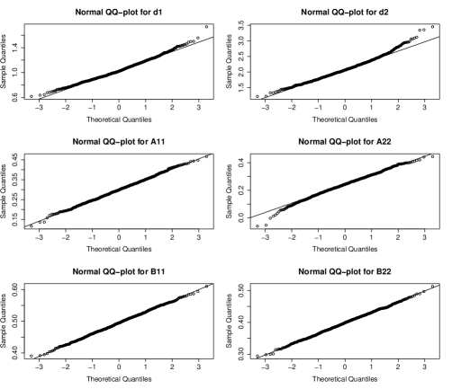
Figure 1: QQ-plots of the standardized sampling distribution of $\widehat{\mbox{\boldmath$\bf\theta$}}$ for the multivariate linear model with true parameter values given by (18) with $n=1000$. Data have been generated by a Gaussian copula with $\phi=0$. Results are based on 1000 runs.

Furthermore, we study the sensitivity of the previous results on the choice of the copula function employed to generate data. This is done by a further simulation setup which utilizes the Clayton copula with parameters $\phi=0$ and 1. The parameter vector $\bf\theta$ is chosen according to (18) and the results of this study are reported in Table 2 and Figure 2 both of which indicate the adequacy of the proposed estimation method.

Sample size	$\phi$	$\hat{d}_{1}$	$\hat{d}_{2}$	$\hat{a}_{11}$	$\hat{a}_{22}$	$\hat{b}_{11}$	$\hat{b}_{22}$	$\hat{a}_{12}$	$\hat{a}_{21}$	$\hat{b}_{12}$	$\hat{b}_{21}$
500	0	1.082	2.173	0.290	0.235	0.495	0.394	0.002	-0.004	0.001	0.002
		(0.220)	(0.423)	(0.077)	(0.104)	(0.049)	(0.050)	(0.093)	(0.076)	(0.044)	(0.049)
	1	1.076	2.156	0.289	0.243	0.494	0.394	0.002	-0.006	$1\cdot 10^{-4}$	-0.001
		(0.215)	(0.413)	(0.087)	(0.112)	(0.058)	(0.054)	(0.106)	(0.089)	(0.049)	(0.057)
1000	0	1.032	2.058	0.298	0.247	0.496	0.398	-0.001	-0.001	$-2\cdot 10^{-4}$	$-1\cdot 10^{-4}$
		(0.145)	(0.299)	(0.051)	(0.070)	(0.034)	(0.034)	(0.065)	(0.056)	(0.029)	(0.035)
	1	1.045	2.077	0.293	0.247	0.497	0.397	0.001	-0.005	$-3\cdot 10^{-4}$	0.001
		(0.151)	(0.286)	(0.059)	(0.078)	(0.040)	(0.038)	(0.074)	(0.064)	(0.035)	(0.041)

Table 2: Simulation results for the multivariate linear model (1) by employing the Clayton copula with parameter $\phi$. True parameter values are given by (18). Standard errors of the estimators are given in parentheses. Results are based on 1000 runs.

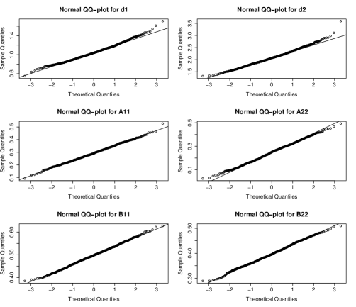
Figure 2: QQ-plots of the standardized sampling distribution of $\widehat{\mbox{\boldmath$\bf\theta$}}$ for the multivariate linear model with true parameter values given by (18) with $n=1000$. Data have been generated by a Clayton copula with $\phi=0$. Results are based on 1000 runs.

Finally Table 3 illustrates simulation results obtained from the linear model where the off-diagonal elements of the matrices ${\mathbf{A}}$ and ${\mathbf{B}}$ are non-zero, i.e. following parameters

$${\mathbf{A}}=\begin{pmatrix}0.3&0.05\\ 0.1&0.25\end{pmatrix},\quad{\mathbf{B}}=\begin{pmatrix}0.5&0.05\\ 0.1&0.4\end{pmatrix}~{}\mbox{and}~{}{\mathbf{d}}=(0.5,1).$$ (19)

Note that these parameter values yield $\||{\bf A}+{\bf B}\||_{2}=0.89<1$ but $\||{\bf A}\||_{1}+\||{\bf B}\||_{1}=1$ (compare Propositions 3.1 and 3.2).

Sample size	$\phi$	$\hat{d}_{1}$	$\hat{d}_{2}$	$\hat{a}_{11}$	$\hat{a}_{22}$	$\hat{b}_{11}$	$\hat{b}_{22}$	$\hat{a}_{12}$	$\hat{a}_{21}$	$\hat{b}_{12}$	$\hat{b}_{21}$
500	0	0.871	1.421	0.289	0.222	0.493	0.396	0.087	0.167	0.051	0.098
		(0.205)	(0.349)	(0.071)	(0.084)	(0.049)	(0.050)	(0.082)	(0.077)	(0.045)	(0.049)
	0.5	0.772	1.116	0.279	0.200	0.494	0.395	0.083	0.161	0.051	0.099
		(0.170)	(0.264)	(0.074)	(0.087)	(0.051)	(0.051)	(0.085)	(0.081)	(0.050)	(0.052)
1000	0	0.803	1.316	0.295	0.222	0.498	0.400	0.083	0.166	0.052	0.099
		(0.134)	(0.236)	(0.052)	(0.057)	(0.036)	(0.032)	(0.054)	(0.054)	(0.030)	(0.036)
	0.5	0.733	1.056	0.286	0.207	0.497	0.396	0.082	0.157	0.048	0.100
		(0.118)	(0.181)	(0.055)	(0.061)	(0.037)	(0.037)	(0.057)	(0.054)	(0.035)	(0.037)

Table 3: Simulation results for the multivariate linear model (1) by employing the Clayton copula with parameter $\phi$. True parameter values are given by (19). Standard errors of the estimators are given in parentheses. Results are based on 1000 runs.

5.2 Simulations for the log-linear model

In this section, we report some limited simulation study results for the case of the log-linear model (4). For this model, the problem of obtaining starting values for the parameter $\bf\theta$ to initiate the maximization of (10) is more challenging. We resort to univariate fits (see Fokianos and Tjøstheim (2011) for details) in the case of diagonal matrices $\mathbf{A}$ and $\mathbf{B}$. In the case of non-diagonal matrices, we can still fit univariate log-linear models to each series and then add an extra step of multivariate least squares estimation to obtain starting values. The parameter values have been chosen by

$${\mathbf{A}}=\begin{pmatrix}-0.3&0\\ 0&0.25\end{pmatrix},\quad{\mathbf{B}}=\begin{pmatrix}0.5&0\\ 0&0.4\end{pmatrix},~{}~{}\mathbf{d}=(0.5,1),$$ (20)

and

$${\mathbf{A}}=\begin{pmatrix}0.4&0\\ 0&0.45\end{pmatrix},\quad{\mathbf{B}}=\begin{pmatrix}0.5&0\\ 0&0.35\end{pmatrix},~{}~{}{\mathbf{d}}=(0.3,0.5).$$ (21)

Furthermore, we employ the Gaussian copula to generate the data with chosen parameter $\phi$ given by 0 and 0.5. The simulation results are shown in Tables 4 and 5. In both cases we note that the estimated parameters are close to their true values, and the approximation improves for larger sample sizes. QQ-plots for the standardized estimated parameters under model (20) when $\phi=0.5$ and sample size of 1000 observations, are shown in Figure 3, and again support asymptotic normality.

Sample size	$\phi$	$\hat{d}_{1}$	$\hat{d}_{2}$	$\hat{a}_{11}$	$\hat{a}_{22}$	$\hat{b}_{11}$	$\hat{b}_{22}$	$\hat{a}_{12}$	$\hat{a}_{21}$	$\hat{b}_{12}$	$\hat{b}_{21}$
500	0	0.510	1.042	-0.302	0.238	0.498	0.3986	$5\cdot 10^{-4}$	0.011	$-1\cdot 10^{-4}$	0.002
		(0.661)	(0.248)	(0.121)	(0.107)	(0.064)	(0.046)	(0.045)	(0.268)	(0.021)	(0.127)
	0.5	0.533	1.027	-0.310	0.242	0.498	0.399	-0.002	0.007	$2\cdot 10^{-4}$	0.002
		(0.699)	(0.238)	(0.118)	(0.105)	(0.068)	(0.047)	(0.045)	(0.280)	(0.022)	(0.131)
1000	0	0.504	1.016	-0.303	0.246	0.496	0.399	$2\cdot 10^{-4}$	-0.001	$3\cdot 10^{-4}$	0.004
		(0.515)	(0.163)	(0.086)	(0.071)	(0.045)	(0.034)	(0.032)	(0.196)	(0.016)	(0.089)
	0.5	0.536	1.005	-0.299	0.250	0.498	0.399	-0.001	-0.010	0.001	-0.001
		(0.502)	(0.166)	(0.091)	(0.071)	(0.045)	(0.032)	(0.031)	(0.196)	(0.015)	(0.091)

Table 4: Simulation results for the multivariate log-linear model (2) by employing the Gaussian copula with parameter $\phi$. True parameter values are given by (20). Standard errors are given in parentheses. Results are based on 1000 runs.

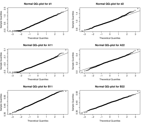
Figure 3: QQ-plots of the standardized sampling distribution of $\widehat{\mbox{\boldmath$\bf\theta$}}$ for the multivariate log-linear model with true parameter values given by (20) with $n=1000$. Data have been generated by a Gaussian copula with $\phi=0.5$. Results are based on 1000 runs.

Sample size	$\phi$	$\hat{d}_{1}$	$\hat{d}_{2}$	$\hat{a}_{11}$	$\hat{a}_{22}$	$\hat{b}_{11}$	$\hat{b}_{22}$	$\hat{a}_{12}$	$\hat{a}_{21}$	$\hat{b}_{12}$	$\hat{b}_{21}$
500	0	0.321	0.522	0.384	0.426	0.505	0.353	0.011	0.006	$-4\cdot 10^{-4}$	$-3\cdot 10^{-4}$
		(0.183)	(0.244)	(0.064)	(0.096)	(0.050)	(0.047)	(0.076)	(0.068)	(0.058)	(0.034)
	0.5	0.326	0.524	0.388	0.428	0.500	0.352	0.013	0.004	-0.004	$-1\cdot 10^{-4}$
		(0.152)	(0.198)	(0.066)	(0.109)	(0.050)	(0.051)	(0.084)	(0.074)	(0.064)	(0.037)
1000	0	0.302	0.518	0.394	0.437	0.501	0.350	0.007	0.006	-0.002	-0.001
		(0.129)	(0.158)	(0.043)	(0.065)	(0.033)	(0.035)	(0.055)	(0.048)	(0.041)	(0.024)
	0.5	0.321	0.521	0.394	0.436	0.502	0.350	0.003	-0.003	0.002	0.001
		(0.109)	(0.132)	(0.046)	(0.068)	(0.035)	(0.035)	(0.057)	(0.052)	(0.045)	(0.027)

Table 5: Simulation results for the multivariate log-linear model (2) by employing the Gaussian copula with parameter $\phi$. True parameter values are given by (21). Standard errors are given in parentheses. Results are based on 1000 runs.

To evaluate the proposed procedure for the copula parameter estimation (see Section A-11) we perform a further simulation study for the linear model (1) using the parameter values defined by (18). The results are reported in Appendix A-12. (Note that for the linear and log-linear model we do not need the copula structure to estimate the parameters $\bf d$, $\bf A$ and $\bf B$.)

5.3 Real data analysis

We fit the linear and log-linear models to a bivariate count time series which consists of the number of transactions per 15 seconds for the stocks Coca-Cola Company (KO) and IBM on September 19th 2005. There are 1551 observations in each of the two series, covering trades from 09:30 to 16:30, excluding the first and last minute of transactions. Figure 4 shows a time series plot of the data and Figure 5 depicts the autocorrelation function and cross- autocorrelation functions. Clearly, the plot of the autocorrelation functions reveals high correlation within and between the individual transaction series. Note further that mean number of transactions is 5.115 and 4.470 , for IBM and KO stocks respectively. The sample variances are 17.315 (IBM) and 12.806 (KO), that is the data clearly shows marginal overdispersion.

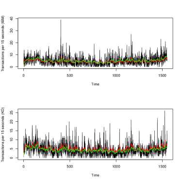
Figure 4: Number of transactions per 15 seconds for IBM (top) and Coca-Cola (bottom) and the respective predicted number of transactions from the linear model (red line) and the log-linear model (green line).

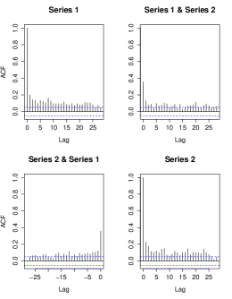
Figure 5: Auto- and cross-correlation function of the transaction data.

Maximization of the quasi log-likelihood function (10), where we have initialized the recursions by a linear regression fit to the data, as it was done for the simulation experiments, yields the following results:

$$\hat{\lambda}_{1,t} = 0.3335+0.6993\hat{\lambda}_{1,t-1}+0.1230\hat{\lambda}_{2,t-1}+0.2027Y_{1,t-1}+0.0150Y_{2,t-1},$$

$$(0.0074)\;\;\;(0.0649)\;\;\;\;\;\;\;\;(0.0007)\;\;\;\;\;\;\;\;(0.2024)\;\;\;\;\;\;\;\;(0.0046)$$

$$\hat{\lambda}_{2,t} = 0.4308+0.0459\hat{\lambda}_{1,t-1}+0.0527\hat{\lambda}_{2,t-1}+0.1594Y_{1,t-1}+0.5635Y_{2,t-1}$$

$$(0.4289)\;\;\;(0.0037)\;\;\;\;\;\;\;\;(0.0005)\;\;\;\;\;\;\;\;(0.0461)\;\;\;\;\;\;\;\;(0.2756)$$

For fitting the log-linear model initialization of the recursions has been done as in Section 5 when considering non-diagonal matrices. The results are as follows:

$$\hat{\nu}_{1,t} = 0.0416+0.9025\hat{\nu}_{1,t-1}-0.0264\hat{\nu}_{2,t-1}+0.0751\log(Y_{1,t-1}+1)+0.0317\log(Y_{2,t-1}+1),$$

$$(2.65\cdot 10^{-5})\;\;\;(4.37\cdot 10^{-5})\;\;(1.30\cdot 10^{-5})\;\;(4.16\cdot 10^{-5})\;\;\;\;\;\;\;\;(3.74\cdot 10^{-5})$$

$$\hat{\nu}_{2,t} = 0.0491-0.0362\hat{\nu}_{1,t-1}+0.8778\hat{\nu}_{2,t-1}+0.0217\log(Y_{1,t-1}+1)+0.0914\log(Y_{2,t-1}+1)$$

$$(2.65\cdot 10^{-4})\;\;\;(3.05\cdot 10^{-6})\;\;(6.70\cdot 10^{-5})\;\;(4.10\cdot 10^{-4})\;\;\;\;\;\;\;\;(1.49\cdot 10^{-3})$$

In both cases, the standard errors given in parentheses underneath the estimated parameters were computed using the robust estimator of the covariance matrix, $\mathbf{H}^{-1}_{n}(\mathbf{\hat{\theta}})\mathbf{G}_{n}(\mathbf{\hat{\theta}})\mathbf{H}^{-1}_{n}(\mathbf{\hat{\theta}})$ where $\mathbf{H}_{n}$ and $\mathbf{G}_{n}$ are given in equation (13) and (14), respectively. The magnitude of the standard errors shows that the feedback process should be considered in both models.
The predictions obtained from both fitted models are denoted by $\hat{Y}_{i,t}=\lambda_{i,t}(\mathbf{\hat{\theta}})$ for $i=1,2$ and are shown in Figure 4. We see that the predictions approximate the observed processes reasonably well.

To examine the model fit, we consider the Pearson residuals, defined by $e_{i,t}=(Y_{i,t}-\lambda_{i,t})/\sqrt{\lambda_{i,t}}$ for $i=1,2$. Under the correct model, the sequence $e_{i,t}$ is a white noise sequence with constant variance. We substitute $\lambda_{i,t}$ by $\lambda_{i,t}(\mathbf{\hat{\theta}})$ to obtain $\hat{e}_{i,t}$. We compute the Pearson residuals for both models and examine their cumulative periodograms. Figure 6 supports the marginal whiteness of the residual process. Finally, the results of the copula estimation are reported in Appendix A-13.

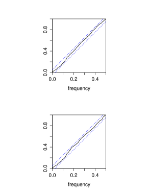
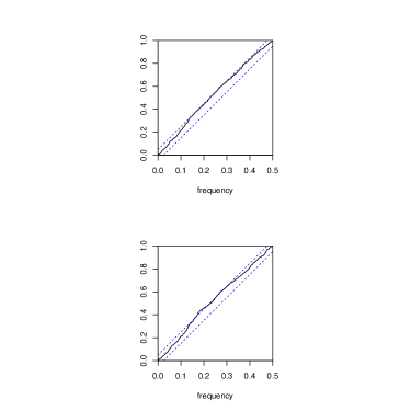
Figure 6: Left:Cumulative periodogram plots of the Pearson residuals from the linear fit of IBM (top) and Coca-Cola (bottom). Right:Cumulative periodogram plots of the Pearson residuals from the log-linear fit of IBM (top) and Coca-Cola (bottom).

6 Discussion

In this work, we have studied the problem of inference and modeling for multivariate count time series. We have proposed models that can accommodate dependence across time and within time series components. Further investigation is required to develop the properties of these multivariate count processes not the least for the copula estimation. In addition, equation (22) motivates a more general framework that can be developed for the analysis of multivariate count time series modes. For instance, a natural generalization, is to consider

$$S_{{\mbox{\boldmath$\bf v$}}}({\mbox{\boldmath$\bf\theta$}})=\sum_{t=1}^{n}\frac{\partial{\mbox{\boldmath$\bf\lambda$}}_{t}}{\partial{\mbox{\boldmath$\bf\theta$}}}{\bf V}^{-1}_{t}(\rho,{\mbox{\boldmath$\bf\lambda$}}_{t}({\mbox{\boldmath$\bf\theta$}}))\Bigl{(}{\bf Y}_{t}-{\mbox{\boldmath$\bf\lambda$}}_{t}(\mbox{\boldmath$\bf\theta$})\Bigr{)},$$ (22)

where the notation is completely analogous to the equations (11) and ${\bf V}^{-1}_{t}(\rho,{\mbox{\boldmath$\bf\lambda$}}_{t}({\mbox{\boldmath$\bf\theta$}}))$ is a $p\times p$ "working" conditional covariance matrix which depend upon the process $\{\mbox{\boldmath$\bf\lambda$}_{t}\}$ and possibly some other parameters $\rho$, as we explain below. Several choices for the working conditional covariance matrix are available in the literature. Here we discuss some of the most commonly used.

1. ${\bf V}={\bf I}_{p}$. The choice of the identity matrix corresponds to a least squares solution to the problem of estimating $\bf\theta$.

2. The $p\times p$ diagonal matrix

   $${\bf D}({\mbox{\boldmath$\bf\lambda$}})=\left(\begin{array}[]{cccc}\lambda_{1,t}&0&\cdots&0\\ 0&\lambda_{2,t}&\cdots&0\\ \cdots&\cdots&\cdots&\cdots\\ 0&0&\cdots&\lambda_{p,t}\\ \end{array}\right)$$

   yields estimating equations (11); that is the score function under independence.

3. The choice

   $${\bf V}(\rho,{\mbox{\boldmath$\bf\lambda$}})=\left(\begin{array}[]{cccc}\lambda_{1,t}&\rho_{12}\sqrt{\lambda_{1,t}}\sqrt{\lambda_{2,t}}&\cdots&\rho_{1p}\sqrt{\lambda_{1,t}}\sqrt{\lambda_{p,t}}\\ \rho_{12}\sqrt{\lambda_{1,t}}\sqrt{\lambda_{2,t}}&\lambda_{2,t}&\cdots&\rho_{2p}\sqrt{\lambda_{2,t}}\sqrt{\lambda_{p,t}}\\ \cdots&\cdots&\cdots&\cdots\\ \rho_{1p}\sqrt{\lambda_{1,t}}\sqrt{\lambda_{p,t}}&\rho_{2p}\sqrt{\lambda_{2,t}}\sqrt{\lambda{p,t}}&\cdots&\lambda_{p,t}\\ \end{array}\right)$$

   yields a constant conditional correlation type of model for multivariate count time series, see Teräsvirta et al. (2010), among others.

We leave this topic for further research by mentioning also the recent work of Francq and Zakoï an (2016) who consider estimation of multivariate volatility models equation by equation.

Appendix

It is easy to see that ${\mbox{\boldmath$\bf\lambda$}}^{\star}=({\bf I}-{\bf A})^{-1}{\bf d}$ is a fixed point of the skeleton (3). The proof of the following lemma is quite analogous to the proof of Fokianos et al. (2009a, Lemma A.1) and it is omitted.

Lemma A-1

Let $\{\mbox{\boldmath$\bf\lambda$}_{t}\}$ be a Markov chain defined by (4) or (5). If $\||{\bf A}\||_{2}<1$, then every point in $[\lambda^{\star}_{1},\infty)\times\ldots\times[\lambda^{\star}_{p},\infty)$ is reachable, where $\lambda^{\star}_{i}$ denotes the $i$’th component of the vector ${\mbox{\boldmath$\bf\lambda$}}^{\star}$.

A-1 Proof of Proposition 3.1

The conditions of $\phi$-irreducibility and the existence of small sets can be proved along the lines of the proof of Fokianos et al. (2009a, Prop. 2.1) provided that $\||{\bf A}\||_{2}<1$. As in the proof of that Proposition we use the Tweedie criterion to prove geometric ergodicity. Define now the test function $V({\bf x})=1+\|{\bf x}\|_{2}^{r}$. Then, we obtain as $\lambda_{i}\rightarrow\infty$, $i=1,2,\ldots,p$,

$$\mbox{E}\left[V(\mbox{\boldmath$\bf\lambda$}_{t}^{m})|{\mbox{\boldmath$\bf\lambda$}}_{t-1}^{m}=\mbox{\boldmath$\bf\lambda$}\right] = 1+\mbox{E}\left[\|{\bf d}+{\bf A}{\mbox{\boldmath$\bf\lambda$}}+{\bf B}{\bf Y}_{t-1}^{m}+{\mbox{\boldmath$\bf\epsilon$}}_{t;m}\|_{2}^{r}\right]$$

$$\sim \mbox{E}\left[\|{\bf A}{\mbox{\boldmath$\bf\lambda$}}+{\bf B}{\bf Y}_{t-1}^{m}\|_{2}^{2}\right]^{\mu},$$

where we assume, without loss of generality, that $\mu=r/2$, $r$ a positive integer. Next,

$$\mbox{E}\left[\|{\bf A}{\mbox{\boldmath$\bf\lambda$}}+{\bf B}{\bf Y}_{t-1}^{m}\|_{2}^{r}\right]=\mbox{E}\left[\Bigl{[}\sum_{i=1}^{p}\left(({\bf A}{\mbox{\boldmath$\bf\lambda$}})_{i}+({\bf B}{\bf Y}_{t-1}^{m})_{i}\right)^{2}\Bigr{]}\right]^{\mu}:=\mbox{E}\left(\sum_{i=1}^{p}C_{i}\right)^{\mu},$$

where $({\bf A}{\mbox{\boldmath$\bf\lambda$}})_{i}$ and $({\bf B}{\bf Y}_{t-1}^{m})_{i}$ are the $i$th components of the vectors ${\bf A}{\mbox{\boldmath$\bf\lambda$}}$ and ${\bf B}{\bf Y}_{t-1}^{m}$, respectively. But

$$\left(\sum_{i=1}^{p}C_{i}\right)^{\mu}=\sum_{i_{1}}\ldots\sum_{i_{p}}\frac{\mu!}{i_{1}!\ldots i_{p}!}C_{1}^{i_{1}}\ldots C_{p}^{i_{p}},$$

where the sum extends over all indices $i_{j},j=1,2,\ldots p$ such that $\sum_{j=1}^{p}i_{j}=\mu$. Successive use of the Cauchy-Schwartz inequality yields

$$\mbox{E}\left(C_{1}^{i_{1}}\ldots C_{p}^{i_{p}}\right)\leq\mbox{E}^{1/2l_{1}}(C_{1}^{2i_{1}l_{1}})\ldots\mbox{E}^{1/2l_{p}}(C_{p}^{2i_{p}l_{p}}),$$

where $1\leq l_{p}\leq 2^{p-2}$, and

$$\mbox{E}\left(C_{k}^{2i_{k}l_{k}}\right)=\mbox{E}\left[({\bf A}{\mbox{\boldmath$\bf\lambda$}})_{k}+({\bf B}{\bf Y}_{t-1}^{m})_{k}\right]^{4i_{k}l_{k}}=\mbox{E}\left[\sum_{j=0}^{4i_{k}l_{k}}{4i_{k}l_{k}\choose j}({\bf A}{\mbox{\boldmath$\bf\lambda$}})_{k}^{j}({\bf B}{\bf Y}_{t-1})_{k}^{4i_{k}l_{k}-j}\right].$$

But using the reasoning on page 26 of Fokianos et al. (2009b), as ${\lambda}_{k}\rightarrow\infty$, $k=1,\ldots,p,$

$$\mbox{E}\left[({\bf B}{\bf Y}_{t-1})_{k}^{4i_{k}l_{k}-j}|{\mbox{\boldmath$\bf\lambda$}}_{t-1}={\mbox{\boldmath$\bf\lambda$}}\right]\sim({\bf{B}}{\mbox{\boldmath$\bf\lambda$}})_{k}^{4i_{k}l_{k}-j}.$$

Hence

$$\mbox{E}^{1/2l_{k}}\left(C_{k}^{2i_{k}l_{k}}\right)\sim\left(({\bf{A}}+{\bf{B}}){\mbox{\boldmath$\bf\lambda$}}\right)_{k}^{2i_{k}},$$

and asymptotically $\mbox{E}\left(C_{1}^{i_{1}}\ldots C_{p}^{i_{p}}\right)\leq\left(({\bf{A}}+{\bf{B}}){\mbox{\boldmath$\bf\lambda$}}\right)_{1}^{2i_{1}}\ldots\left(({\bf{A}}+{\bf{B}}){\mbox{\boldmath$\bf\lambda$}}\right)_{p}^{2i_{p}}$. Therefore we obtain that

$$\mbox{E}\left(\sum_{i=1}^{p}C_{i}\right)^{\mu} \leq \sum_{i_{1}}\ldots\sum_{i_{p}}\frac{\mu!}{i_{1}!\ldots i_{p}!}\left[\left(({\bf{A}}+{\bf{B}}){\mbox{\boldmath$\bf\lambda$}}\right)_{1}^{2}\right]^{i_{1}}\ldots\left[\left(({\bf{A}}+{\bf{B}}){\mbox{\boldmath$\bf\lambda$}}\right)_{p}^{2}\right]^{i_{p}}$$

$$= \left[\sum_{j=1}^{p}\left(({\bf{A}}+{\bf{B}}){\mbox{\boldmath$\bf\lambda$}}\right)^{2}_{j}\right]^{\mu}=\left(\||({\bf A}+{\bf{B}}){\mbox{\boldmath$\bf\lambda$}}\||_{2}^{2}\right)^{\mu}\leq\left(\||({\bf A}+{\bf{B}})\||_{2}^{2}\|{\mbox{\boldmath$\bf\lambda$}}\|_{2}^{2}\right)^{\mu}$$

which, using the Tweedie criterion as in Fokianos et al. (2009a, Prop. 2.1), implies that $\||{\bf A}+{\bf{B}}\||_{2}<1$ is a sufficient condition, and the proposition thus holds.

A-2 Proof of Lemma 3.1

To prove the first item of the Lemma, note that

$$\|\mbox{E}({\mbox{\boldmath$\bf\lambda$}}_{t}^{m}-{\mbox{\boldmath$\bf\lambda$}}_{t})\|_{2} = \|{\bf A}\mbox{E}({\mbox{\boldmath$\bf\lambda$}}_{t-1}^{m}-{\mbox{\boldmath$\bf\lambda$}}_{t-1})+{\bf B}\mbox{E}({\bf Y}_{t-1}^{m}-{\bf Y}_{t-1})+\mbox{E}({\mbox{\boldmath$\bf\epsilon$}}_{t}^{m})\|_{2}$$

$$= \|{\bf A}\mbox{E}\left({\mbox{\boldmath$\bf\lambda$}}_{t-1}^{m}-{\mbox{\boldmath$\bf\lambda$}}_{t-1}\right)+{\bf B}\left[\mbox{E}\left[\mbox{E}\left(({\bf Y}_{t-1}^{m}|{\cal{F}}_{t-1;m}^{\bf{Y},\mbox{\boldmath$\bf\lambda$}})\right)\right]-\mbox{E}\left[\mbox{E}\left({\bf Y}_{t-1}|{\cal{F}}_{t-1}^{\bf{Y},\mbox{\boldmath$\bf\lambda$}}\right)\right]\right]+\mbox{E}({\mbox{\boldmath$\bf\epsilon$}}_{t}^{m})\|_{2}$$

$$\leq \||{\bf A}+{\bf B}\||_{2}\|\mbox{E}({\mbox{\boldmath$\bf\lambda$}}_{t-1}^{m}-{\mbox{\boldmath$\bf\lambda$}}_{t-1})\|_{2}+\|\mbox{E}({\mbox{\boldmath$\bf\epsilon$}}_{t}^{m})\|_{2},$$

where ${\cal{F}}_{t-1}^{\bf{Y},\mbox{\boldmath$\bf\lambda$}}$ and ${\cal{F}}_{t-1;m}^{\bf{Y},\mbox{\boldmath$\bf\lambda$}}$ are the $\sigma$-algebras generated by $\{{\mbox{\boldmath$\bf\lambda$}}_{s},s\leq t\ \}$ and $\{{\mbox{\boldmath$\bf\lambda$}}_{s}^{m},s\leq t\ \}$, respectively. By recursion and the fact that $\|\mbox{E}({\mbox{\boldmath$\bf\epsilon$}}_{t}^{m})\|_{2}\leq c_{m}$ which tends to zero as $m\rightarrow\infty$ we obtain the desired result. To prove the second statement, note that as $m\rightarrow\infty$,

$$\mbox{E}\|({\mbox{\boldmath$\bf\lambda$}}_{t}^{m}-{\mbox{\boldmath$\bf\lambda$}}_{t})\|_{2}^{2} \sim \mbox{E}\|{\bf A}({\mbox{\boldmath$\bf\lambda$}}_{t-1}^{m}-{\mbox{\boldmath$\bf\lambda$}}_{t-1})+{\bf B}({\bf Y}_{t-1}^{m}-{\bf Y}_{t-1})\|_{2}^{2}.$$

Let $\Delta_{t-1}{\mbox{\boldmath$\bf\lambda$}}={\mbox{\boldmath$\bf\lambda$}}_{t-1}^{m}-{\mbox{\boldmath$\bf\lambda$}}_{t-1}$ and $\Delta_{t-1}{\bf Y}={\bf Y}_{t-1}^{m}-{\bf Y}_{t-1}$ , then

$$\mbox{E}\|({\mbox{\boldmath$\bf\lambda$}}_{t}^{m}-{\mbox{\boldmath$\bf\lambda$}}_{t})\|_{2}^{2} \sim \mbox{E}\left[\Delta_{t-1}{\mbox{\boldmath$\bf\lambda$}}^{T}{\bf A}^{T}{\bf A}\Delta_{t-1}{\mbox{\boldmath$\bf\lambda$}}+\Delta_{t-1}{\mbox{\boldmath$\bf\lambda$}}^{T}{\bf A}^{T}{\bf B}\Delta_{t-1}{\bf Y}+\Delta_{t-1}{\bf Y}^{T}{\bf B}^{T}{\bf A}\Delta_{t-1}{\mbox{\boldmath$\bf\lambda$}}+\Delta_{t-1}{\bf Y}^{T}{\bf B}^{T}{\bf B}\Delta_{t-1}{\bf Y}\right]$$

$$= \mbox{E}\left[\Delta_{t-1}{\mbox{\boldmath$\bf\lambda$}}^{T}{\bf C}\Delta_{t-1}{\mbox{\boldmath$\bf\lambda$}}+\Delta_{t-1}{\mbox{\boldmath$\bf\lambda$}}^{T}{\bf D}\Delta_{t-1}{\bf Y}+\Delta_{t-1}{\bf Y}^{T}{\bf D}^{T}\Delta_{t-1}{\mbox{\boldmath$\bf\lambda$}}+\Delta_{t-1}{\bf Y}^{T}{\bf E}\Delta_{t-1}{\bf Y}\right]$$

$$:= \sum_{i=1}^{p}\sum_{j=1}^{p}\mbox{E}\left[c_{ij}\Delta_{t-1}\lambda_{i}\Delta_{t-1}\lambda_{j}+d_{ij}\Delta_{t-1}\lambda_{i}\Delta_{t-1}Y_{j}+d_{ji}\Delta_{t-1}\lambda_{i}\Delta_{t-1}Y_{j}+e_{ij}\Delta_{t-1}Y_{i}\Delta_{t-1}Y_{j}\right],$$

where ${\bf C}={\bf A}^{T}{\bf A}$, ${\bf D}={\bf A}^{T}{\bf B}$ and ${\bf E}={\bf B}^{T}{\bf B}$. By using properties of conditional expectation as before, we obtain

$$\mbox{E}\left[d_{ij}\Delta_{t-1}\lambda_{i}\Delta_{t-1}Y_{j}+d_{ji}\Delta_{t-1}\lambda_{i}\Delta_{t-1}Y_{j}\right] = \mbox{E}\left[d_{ij}\Delta_{t-1}\lambda_{i}\Delta_{t-1}\lambda_{j}+d_{ji}\Delta_{t-1}\lambda_{i}\Delta_{t-1}\lambda_{j}\right]$$

In addition, following the proof in Fokianos et al. (2009a, Lemma 2.1), and using the above conditioning argument,

$$\mbox{E}\left(\Delta_{t-1}Y_{i}^{2}\right)=\mbox{E}\left(\Delta_{t-1}\lambda_{i}\right)^{2}+2\delta_{i,m},$$

where $\delta_{i,m}\rightarrow 0$, as $m\rightarrow\infty$. For the cross-terms we have to condition on the copula structure, ${\cal{F}}_{t-1;m}^{\bf{Y},\mbox{\boldmath$\bf\lambda$}}$, as well i.e.

$$\mbox{E}\left(\Delta_{t-1}Y_{i}\Delta_{t-1}Y_{j}\right) = \mbox{E}\left[\mbox{E}\left[\Delta_{t-1}Y_{i}\Delta_{t-1}Y_{j}|{\cal{F}}_{t-1;m}^{\bf{Y},\mbox{\boldmath$\bf\lambda$}},{\cal{F}}_{t-1}^{\bf{Y},\mbox{\boldmath$\bf\lambda$}}\right]\right]=\mbox{E}\left(\Delta_{t-1}\lambda_{i}\Delta_{t-1}\lambda_{j}\right).$$

Collecting all previous results, we obtain

$$\mbox{E}\|\left({\mbox{\boldmath$\bf\lambda$}}_{t}^{m}-{\mbox{\boldmath$\bf\lambda$}}_{t})\right)\|_{2}^{2} = \mbox{E}\|({\bf A}+{\bf B})({\mbox{\boldmath$\bf\lambda$}}_{t-1}^{m}-{\mbox{\boldmath$\bf\lambda$}}_{t-1})\|_{2}^{2}+D_{m}$$

$$\leq \||{\bf A}+{\bf B}\||_{2}^{2}\mbox{E}\|({\mbox{\boldmath$\bf\lambda$}}_{t-1}^{m}-{\mbox{\boldmath$\bf\lambda$}}_{t-1})\|_{2}^{2}+D_{m},$$

where $D_{m}\rightarrow 0$ as $m\rightarrow\infty$. The last two statements are proved using straightforward adaptation of the proof of Fokianos et al. (2009a, Lemma 2.1).

A-3 Proof of Proposition 3.2

The proof is based on Doukhan and Wintenberger (2008, Thm. 3.1) and parallels the proof given by Doukhan et al. (2012b). In proving weak dependence, we define the $\mbox{\boldmath$\bf X$}_{t}=(\mbox{\boldmath$\bf Y$}^{T}_{t},\mbox{\boldmath$\bf\lambda$}^{T}_{t})^{T}$ and we employ the norm $\|\mbox{\boldmath$\bf x$}\|_{\epsilon}=\|\mbox{\boldmath$\bf y$}\|_{1}+\epsilon\|\mbox{\boldmath$\bf\lambda$}\|_{1}$, where $\epsilon$ is not necessarily small. Then, the contraction property is verified by noting that $\mbox{\boldmath$\bf X$}_{t}=F(\mbox{\boldmath$\bf X$}^{T}_{t-1},\mbox{\boldmath$\bf N$}^{T}_{t})$ where $\mbox{\boldmath$\bf N$}_{t}$ is an iid sequence of $p$-variate copula Poisson processes and choosing $\epsilon=\||\mbox{\boldmath$\bf A$}\||_{1}/\||\mbox{\boldmath$\bf B$}\||_{1}$. This proves that $\mbox{E}[\|\mbox{\boldmath$\bf Y$}_{t}\|_{1}]<\infty$ and $\mbox{E}[\|\mbox{\boldmath$\bf\lambda$}_{t}\|_{1}]<\infty$.

To show finiteness of moments we will be using induction and a different technique than the method used in Doukhan et al. (2012b). More precisely, suppose that $\mbox{E}[\|\mbox{\boldmath$\bf Y$}_{t}\|^{r-1}_{r-1}]<\infty$ and $\mbox{E}[\|\mbox{\boldmath$\bf\lambda$}_{t}\|^{r-1}_{r-1}]<\infty$ for $r\in\mathbb{N}$ and $r>1$. Then consider the $i$-th component of $\mbox{\boldmath$\bf Y$}_{t}$. But

$$\mbox{E}\Bigl{[}Y^{r}_{i,t}\mid{\cal F}^{\mbox{\boldmath$\bf Y$},\mbox{\boldmath$\bf\lambda$}}_{t-1}\Bigr{]} \leq \mbox{E}\Bigl{[}(Y_{i,t})_{r}\mid{\cal F}^{\mbox{\boldmath$\bf Y$},\mbox{\boldmath$\bf\lambda$}}_{t-1}\Bigr{]}+\sum_{k=1}^{r-1}|\delta_{ik}(r)|\mbox{E}\Bigl{[}Y^{k}_{i,t}\mid{\cal F}^{\mbox{\boldmath$\bf Y$},\mbox{\boldmath$\bf\lambda$}}_{t-1}\Bigr{]}$$

$$= \lambda^{r}_{i,t}+\sum_{k=1}^{r-1}|\delta_{ik}(r)|\mbox{E}\Bigl{[}Y^{k}_{i,t}\mid{\cal F}^{\mbox{\boldmath$\bf Y$},\mbox{\boldmath$\bf\lambda$}}_{t-1}\Bigr{]},$$

where $(x)_{r}=x(x-1)....(x-r+1)$, $\{\delta_{jk}(r),~{}k=1,2,\ldots,r-1\}$ are some constants and the first line follows from properties of $(x)_{r}$ while the second line follows form properties of the Poisson distribution. By taking expectations and using the $c_{r}$-inequality, we obtain that

$$\mbox{E}^{1/r}\Bigl{[}Y^{r}_{i,t}\Bigr{]} \leq \mbox{E}^{1/r}\Bigl{[}\lambda^{r}_{i,t}\Bigr{]}+\sum_{k=1}^{r-1}|\delta_{ik}(r)|^{1/r}\mu_{i},$$

where $\mu_{i}=\max_{k<r}\mbox{E}\Bigl{[}Y^{k}_{i,t}\mid{\cal F}^{\mbox{\boldmath$\bf Y$},\mbox{\boldmath$\bf\lambda$}}_{t-1}\Bigr{]}$, which exists by the induction hypothesis. But

$$\mbox{E}(\lambda_{i,t}^{r})\leq\mbox{E}(Y_{i,t}^{r}),$$

because of the properties of the linear model. Therefore, we obtain that (because of (3))

$$\mbox{E}^{1/r}[Y_{i,t}^{r}]\leq d_{i}+\sum_{j=1}^{p}a_{ij}\mbox{E}^{1/r}[Y_{i,t}^{r}]+\sum_{j=1}^{p}b_{ij}\mbox{E}^{1/r}[Y_{i,t}^{r}]+\sum_{k=1}^{r-1}|\delta_{ik}(r)|^{1/r}\mu_{i},$$

and by summing up, using the definition of $\||.\||_{1}$ and its properties, we obtain that

$$\sum_{i=1}^{p}\mbox{E}^{1/r}[Y_{i,t}^{r}]\leq\sum_{i=1}^{p}d_{i}+(\||A\||_{1}+\||B\||_{1})\sum_{i=1}^{p}\mbox{E}^{1/r}[Y_{i,t}^{r}]+\sum_{i=1}^{p}\sum_{k=1}^{r-1}|\delta_{ik}(r)|^{1/r}\mu_{i}.$$

A-4 Proof of Lemma 3.2

We will prove the second and fourth conclusion as the other results follow from Fokianos and Tjøstheim (2011) and the proof of Lemma 3.1. But to prove the second statement, note that

$$\mbox{E}\|({\mbox{\boldmath$\bf\nu$}}_{t}^{m}-{\mbox{\boldmath$\bf\nu$}}_{t})\|_{2}^{2} = \mbox{E}\|{\bf A}\mbox{E}({\mbox{\boldmath$\bf\nu$}}_{t-1}^{m}-{\mbox{\boldmath$\bf\nu$}}_{t-1})+{\bf B}\mbox{E}(\log({\bf Y}_{t-1}^{m}+\mbox{\boldmath$\bf 1$}_{p})-\log({\bf Y}_{t-1}+\mbox{\boldmath$\bf 1$}_{p}))+\mbox{E}({\mbox{\boldmath$\bf\epsilon$}}_{t}^{m})\|_{2}^{2}$$

$$\leq \||{\bf A}\||_{2}^{2}\mbox{E}\|{\mbox{\boldmath$\bf\nu$}}_{t-1}^{m}-{\mbox{\boldmath$\bf\nu$}}_{t-1}\|_{2}^{2}+\||{\bf B}\||_{2}^{2}\mbox{E}\|\log({\bf Y}_{t-1}^{m}+\mbox{\boldmath$\bf 1$}_{p})-\log({\bf Y}_{t-1}+\mbox{\boldmath$\bf 1$}_{p})\|_{2}^{2}$$

$$+ 2\||{\bf A}\||_{2}\||{\bf B}\||_{2}\sqrt{\mbox{E}\|{\mbox{\boldmath$\bf\nu$}}_{t-1}^{m}-{\mbox{\boldmath$\bf\nu$}}_{t-1}\|_{2}^{2}\mbox{E}\|\log({\bf Y}_{t-1}^{m}+\mbox{\boldmath$\bf 1$}_{p})-\log({\bf Y}_{t-1}+\mbox{\boldmath$\bf 1$}_{p})|_{2}^{2}}+\kappa c_{m}^{2},$$

where $\kappa>0$. Consider now the $\mbox{E}(\log(Y_{j,t-1}^{m}+1)-\log(Y_{j,t-1}))^{2}$, $j=1,2,\ldots,p$. Then, following the proof of Fokianos and Tjøstheim (2011, Lemma 2.1) and assuming without loss of generality that $\lambda_{j,t-1}^{m}\geq\lambda_{j,t-1}$ we obtain that $((Y_{j,t-1}^{m}+1)/(Y_{j,t-1}+1)\geq 1$. Therefore by using Jensen’s inequality (by employing the function $(\log x)^{2}$) we obtain that

$$\mbox{E}\left[\log\frac{Y_{j,t-1}^{m}+1}{Y_{j,t-1}+1}\right]^{2}\leq\left[\log\mbox{E}\left(\frac{Y_{j,t-1}^{m}+1}{Y_{j,t-1}+1}\right)^{2}\right].$$

But according to Fokianos and Tjøstheim (2011, p. 576) the right hand side of the above inequality is bounded by $\mbox{E}(\nu_{j,t-1}^{m}-\nu_{j;t-1})^{2}$ for $j=1,2,\ldots,p$. Hence, the conclusion of the Lemma follows again by the same arguments used in the proof of Lemma 3.1.

To prove the fourth result, we follow Fokianos and Tjøstheim (2011, pp. 576-577). Consider the test function $V({\bf x})=\exp(r\|{\bf x}\|_{2})$ for $r\in\mathbb{N}$. Set $b=r\||\mbox{\boldmath$\bf B$}\||_{2}$. Then

$$\mbox{E}[\exp(r\|\mbox{\boldmath$\bf\nu$}^{m}_{t}\|_{2})\mid\mbox{\boldmath$\bf\nu$}^{m}_{t-1}=\mbox{\boldmath$\bf\nu$}] \leq \exp(r(\|\mbox{\boldmath$\bf d$}\|_{2}+\||\mbox{\boldmath$\bf A$}\||_{2}\|\mbox{\boldmath$\bf\nu$}\|_{2}))\mbox{E}[\exp(r\||\mbox{\boldmath$\bf B$}\||_{2}\|\log(\mbox{\boldmath$\bf Y$}^{m}_{t-1}+\mbox{\boldmath$\bf 1$}_{p})\|_{2})\mid\mbox{\boldmath$\bf\nu$}^{m}_{t-1}=\mbox{\boldmath$\bf\nu$}].$$

However

$$\mbox{E}\Bigl{[}\exp\Bigl{(}b\|\log(\mbox{\boldmath$\bf Y$}^{m}_{t-1}+\mbox{\boldmath$\bf 1$}_{p})\|_{2}\Bigr{)}|\mbox{\boldmath$\bf\nu$}^{m}_{t-1}=\mbox{\boldmath$\bf\nu$}\Bigr{]} = \mbox{E}\left\{\exp\Bigl{[}b\Bigl{(}\sum_{i=1}^{p}\log^{2}(Y^{m}_{i,t-1}+1)\Bigr{)}^{1/2}\Bigr{]}|\mbox{\boldmath$\bf\nu$}^{m}_{t-1}=\mbox{\boldmath$\bf\nu$}\right\}$$

$$= \mbox{E}\left\{\exp\Bigl{[}b\Bigl{(}\sum_{i=1}^{p}\Bigl{(}\nu_{i}+\Bigl{(}\frac{\log(Y^{m}_{i,t-1}+1)}{\exp(\nu_{i})}\Bigr{)}\Bigr{)}^{2}\Bigr{)}^{1/2}\bigl{]}|\mbox{\boldmath$\bf\nu$}^{m}_{t-1}=\mbox{\boldmath$\bf\nu$}\right\}.$$

But

$$\mbox{Var}\Bigl{[}\frac{Y^{m}_{t}+1}{\exp(\nu_{i})}\mid\mbox{\boldmath$\bf\nu$}^{m}_{t-1}=\mbox{\boldmath$\bf\nu$}\Bigr{]}=\exp(-\nu_{i})\rightarrow 0,$$ (A-1)

provided that $\nu_{i}\rightarrow\infty$ for all $i=1,2,\ldots,p$. Therefore we have that

$$\mbox{Var}\Bigl{[}\log\Bigr{(}\frac{Y^{m}_{t}+1}{\exp(\nu_{i})}\Bigl{)}\mid\mbox{\boldmath$\bf\nu$}^{m}_{t-1}=\mbox{\boldmath$\bf\nu$}\Bigr{]}\rightarrow 0,$$

by the delta-method for moments and provided that $\nu_{i}\rightarrow\infty$ for all $i=1,2,\ldots,p$. Using now the multivariate delta-method and Cauchy-Schwartz inequality to the function $g(x_{1},\ldots,x_{p})=\exp(b(\sum_{i}^{p}(\nu_{i}+x_{i})^{2})^{1/2})$ (with some abuse of notation), we obtain that

$$\mbox{Var}\left\{\exp\Bigl{[}b\Bigl{(}\sum_{i=1}^{p}\Bigl{(}\nu_{i}+\Bigl{(}\frac{\log(Y^{m}_{i,t-1}+1)}{\exp(\nu_{i})}\Bigr{)}\Bigr{)}^{2}\Bigr{)}^{1/2}\bigl{]}|\mbox{\boldmath$\bf\nu$}^{m}_{t-1}=\mbox{\boldmath$\bf\nu$}\right\}\rightarrow 0.$$

However

$$\mbox{E}\Bigl{[}\frac{Y^{m}_{t}+1}{\exp(\nu_{i})}\mid\mbox{\boldmath$\bf\nu$}^{m}_{t-1}=\mbox{\boldmath$\bf\nu$}\Bigr{]}\sim 1$$ (A-2)

provided that $\nu_{i}\rightarrow\infty$ for all $i=1,2,\ldots,p$. Therefore, asymptotically, we obtain that

$$\mbox{E}\Bigl{[}\exp\Bigl{(}b\|\log(\mbox{\boldmath$\bf Y$}^{m}_{t-1}+\mbox{\boldmath$\bf 1$}_{p})\|_{2}\Bigr{)}|\mbox{\boldmath$\bf\nu$}^{m}_{t-1}=\mbox{\boldmath$\bf\nu$}\Bigr{]}\sim\exp(b\|\mbox{\boldmath$\bf\nu$}\|_{2}).$$

To complete the proof, we note that the above calculations show that

$$\mbox{E}\Bigl{[}\exp(r\|\mbox{\boldmath$\bf\nu$}^{m}_{t})\|_{2})|\mbox{\boldmath$\bf\nu$}^{m}_{t-1}=\mbox{\boldmath$\bf\nu$}]\leq\exp(r(\||\mbox{\boldmath$\bf A$}_{2}\||_{2}+\||\mbox{\boldmath$\bf B$}_{2}\||_{2}-1)\|\mbox{\boldmath$\bf\nu$}\|_{2})\exp(r\|\mbox{\boldmath$\bf\nu$}\|_{2}).$$

Therefore, the conclusion follows as in Fokianos and Tjøstheim (2011, pp. 576-577).

A-5 Proof of Proposition 3.4

For the log-linear model we prove weak dependence by the following method. Set $Y_{j,t}=N_{j,t}(\exp(\nu_{j,t}))$, $j=1,2,\ldots,p$. Then setting $Z_{j,t}=\log(1+Y_{j,t})$ we have for $\mbox{\boldmath$\bf X$}_{t}=(\mbox{\boldmath$\bf Z$}_{t},\mbox{\boldmath$\bf\nu$}_{t})$ with $\mbox{\boldmath$\bf Z$}_{t}=(Z_{j,t},j=1,2,\ldots,p)$ and $N_{t}=(N_{j,t},j=1,2,\ldots,d)$ that

$$\mbox{\boldmath$\bf X$}_{t}=(\mbox{\boldmath$\bf Z$}_{t},\mbox{\boldmath$\bf\nu$}_{t})=F(\mbox{\boldmath$\bf X$}^{T}_{t-1},\mbox{\boldmath$\bf N$}^{T}_{t}),$$

where $\mbox{\boldmath$\bf N$}_{t}=(N_{j,t},j=1,2,\ldots,p)$ iid copula $p$-variate Poisson processes. Then using again the same arguments as in Doukhan et al. (2012b) we obtain (with the same norm) that

$$\mbox{E}\left[\|F(\mbox{\boldmath$\bf x$},\mbox{\boldmath$\bf N$})-F(\mbox{\boldmath$\bf x$}^{\star},\mbox{\boldmath$\bf N$})\|_{\epsilon}\right] \leq \sum_{j=1}^{p}\|\Bigl{(}\mbox{\boldmath$\bf A$}(\mbox{\boldmath$\bf\nu$}-\mbox{\boldmath$\bf\nu$}^{\star})\Bigr{)}_{j}\|_{1}+\sum_{j=1}^{p}\|\Bigl{(}\mbox{\boldmath$\bf B$}(\mbox{\boldmath$\bf\zeta$}-\mbox{\boldmath$\bf\zeta$}^{\star})\Bigr{)}_{j}\|_{1}$$

$$+ \epsilon\Bigl{(}\|\mbox{\boldmath$\bf A$}(\nu-\nu^{\star})\|_{1}+\|\mbox{\boldmath$\bf B$}(\mbox{\boldmath$\bf\zeta$}-\mbox{\boldmath$\bf\zeta$}^{\star})\|_{1}\Bigr{)}$$

$$\leq (1+\epsilon)\Bigl{(}\||\mbox{\boldmath$\bf A$}\||_{1}\mbox{\boldmath$\bf\nu$}-\mbox{\boldmath$\bf\nu$}^{\star}\|_{1}+\||\mbox{\boldmath$\bf B$}\||_{1}\|\mbox{\boldmath$\bf\zeta$}-\mbox{\boldmath$\bf\zeta$}^{\star}\|_{1}\Bigr{)},$$

where the first inequality follows from Fokianos and Tjøstheim (2011, pp.575–576). The results now follow as in Doukhan et al. (2012b). Now we show existence of moments for the log-linear model. Suppose that $r\in\mathbb{N}$. Then

$$\mbox{E}[\exp(r\|\mbox{\boldmath$\bf\nu$}_{t}\|_{1})\mid\mbox{\boldmath$\bf\nu$}_{t-1}=\mbox{\boldmath$\bf\nu$}] \leq \exp(r(\|\mbox{\boldmath$\bf d$}\|_{1}+\||\mbox{\boldmath$\bf A$}\||_{1}\|\mbox{\boldmath$\bf\nu$}\|_{1}))\mbox{E}[\exp(r\||\mbox{\boldmath$\bf B$}\||_{1}\|\mbox{\boldmath$\bf Z$}_{t-1}\|_{1})\mid\mbox{\boldmath$\bf\nu$}_{t-1}=\mbox{\boldmath$\bf\nu$}]$$

With $b=r\||\mbox{\boldmath$\bf B$}\||_{1}$, for the second factor of the right hand side we obtain that

$$\mbox{E}\Bigl{[}\exp\Bigl{(}b\|\mbox{\boldmath$\bf Z$}_{t-1}\|_{1}\Bigr{)}\mid\mbox{\boldmath$\bf\nu$}_{t-1}=\mbox{\boldmath$\bf\nu$}\Bigr{]}=\exp(b\|\mbox{\boldmath$\bf\nu$}\|_{1})\mbox{E}\Bigl{[}\prod_{i=1}^{p}\Bigl{(}\frac{Y_{i,t-1}+1}{\exp(\nu_{i})}\Bigr{)}^{b}\mid\mbox{\boldmath$\bf\nu$}_{t-1}=\mbox{\boldmath$\bf\nu$}\Bigr{]}$$

But from the proof of Lemma 3.2 (see eq. (A-1)) and using similar arguments

$$\mbox{Var}\Bigl{[}\prod_{i=1}^{p}\Bigl{(}\frac{Y_{i,t-1}+1}{\exp(\nu_{i})}\Bigr{)}^{b}\mid\mbox{\boldmath$\bf\nu$}_{t-1}=\mbox{\boldmath$\bf\nu$}\Bigr{]}\rightarrow 0,$$

provided that $\nu_{i}\rightarrow\infty$, for all $i=1,2\ldots,p$. In addition, because of (A-2) and the multivariate delta-method of moments

$$\mbox{E}\Bigl{[}\prod_{i=1}^{p}\Bigl{(}\frac{Y_{i,t-1}+1}{\exp(\nu_{i})}\Bigr{)}^{b}\mid\mbox{\boldmath$\bf\nu$}_{t-1}=\mbox{\boldmath$\bf\nu$}\Bigr{]}\rightarrow 1,$$

provided that $\nu_{i}\rightarrow\infty$, for all $i=1,2\ldots,p$. The above two displays show that

$$\mbox{E}\Bigl{[}\exp\Bigl{(}b\|\mbox{\boldmath$\bf Z$}_{t-1}\|_{1}\Bigr{)}\mid\mbox{\boldmath$\bf\nu$}_{t-1}=\mbox{\boldmath$\bf\nu$}\Bigr{]}\sim\exp(b\|\mbox{\boldmath$\bf\nu$}\|_{1}),$$

as required.

A-6 Proof of Lemma 4.1

In what follows we drop notation that depends on $\bf\theta$ because all quantities are evaluated at the true parameter $\mbox{\boldmath$\bf\theta$}_{0}$. The notation $C$ refers to a generic constant. Initially, we show that

$$\Bigl{\|}\Bigl{|}\frac{\partial\mbox{\boldmath$\bf\lambda$}_{t}^{m}}{\partial\mbox{\boldmath$\bf d$}^{T}}-\frac{\partial\mbox{\boldmath$\bf\lambda$}_{t}}{\partial\mbox{\boldmath$\bf d$}^{T}}\Bigr{\|}\Bigr{|}_{2}<\gamma_{m},~{}a.s,$$ (A-3)

for some positive sequence $\gamma_{m}\rightarrow 0$, as $m\rightarrow\infty$. Using the first equation of (12) we obtain that

$$\Bigl{\|}\Bigl{|}\frac{\partial\mbox{\boldmath$\bf\lambda$}_{t}^{m}}{\partial\mbox{\boldmath$\bf d$}^{T}}-\frac{\partial\mbox{\boldmath$\bf\lambda$}_{t}}{\partial\mbox{\boldmath$\bf d$}^{T}}\Bigr{\|}\Bigr{|}_{2} \leq \||\mbox{\boldmath$\bf A$}\||_{2}\Bigl{\|}\Bigl{|}\frac{\partial\mbox{\boldmath$\bf\lambda$}_{t-1}^{m}}{\partial\mbox{\boldmath$\bf d$}^{T}}-\frac{\partial\mbox{\boldmath$\bf\lambda$}_{t-1}}{\partial\mbox{\boldmath$\bf d$}^{T}}\Bigr{\|}\Bigr{|}_{2}$$

and therefore, by repeated substitution, (A-3) follows since $\||\mbox{\boldmath$\bf A$}\||_{2}<1$ and the results of Lemma 3.1. Similarly,

$$\Bigl{\|}\Bigl{|}\frac{\partial\mbox{\boldmath$\bf\lambda$}_{t}^{m}}{\partial\operatorname{vec}^{T}(\mbox{\boldmath$\bf A$})}-\frac{\partial\mbox{\boldmath$\bf\lambda$}_{t}}{\partial\operatorname{vec}^{T}(\mbox{\boldmath$\bf A$})}\Bigr{\|}\Bigr{|}_{2}\leq\gamma_{m},~{}a.s.$$ (A-4)

Indeed, using the second equation of (12), we obtain that

$$\Bigl{\|}\Bigl{|}\frac{\partial\mbox{\boldmath$\bf\lambda$}_{t}^{m}}{\partial\operatorname{vec}^{T}(\mbox{\boldmath$\bf A$})}-\frac{\partial\mbox{\boldmath$\bf\lambda$}_{t}}{\partial\operatorname{vec}^{T}(\mbox{\boldmath$\bf A$})}\Bigr{\|}\Bigr{|}_{2} \leq \sqrt{p}\|\mbox{\boldmath$\bf\lambda$}_{t-1}^{m}-\mbox{\boldmath$\bf\lambda$}_{t-1}\|_{2}+\||\mbox{\boldmath$\bf A$}\||_{2}\Bigl{\|}\Bigl{|}\frac{\partial\mbox{\boldmath$\bf\lambda$}_{t-1}^{m}}{\partial\operatorname{vec}^{T}(\mbox{\boldmath$\bf A$})}-\frac{\partial\mbox{\boldmath$\bf\lambda$}_{t-1}}{\partial\operatorname{vec}^{T}(\mbox{\boldmath$\bf A$})}\Bigr{\|}\Bigr{|}_{2},$$

where the first bound comes from the fact that in terms of the Frobenious matrix norm $\||\mbox{\boldmath$\bf I$}_{p}\||_{F}=\sqrt{p}$. Therefore, by Lemma 3.1 we obtain the desired result. Finally, it can be shown quite analogously (by using again Lemma (3.1)) that

$$\Bigl{\|}\Bigl{|}\frac{\partial\mbox{\boldmath$\bf\lambda$}_{t}^{m}}{\partial\operatorname{vec}^{T}(\mbox{\boldmath$\bf B$})}-\frac{\partial\mbox{\boldmath$\bf\lambda$}_{t}}{\partial\operatorname{vec}^{T}(\mbox{\boldmath$\bf B$})}\Bigr{\|}\Bigr{|}_{2}\leq\gamma_{m},~{}a.s.$$ (A-5)

To prove the lemma, we consider the $d\times d$ matrix difference

$$\Bigl{\|}\Bigl{|}s_{t}^{m}(s_{t}^{m})^{T}-s_{t}s_{t}^{T}\Bigr{\|}\Bigr{|}_{2} = \Bigl{\|}\Bigl{|}(s_{t}^{m}-s_{t})(s_{t}^{m})^{T}+s_{t}(s_{t}^{m}-s_{t})^{T}\Bigr{\|}\Bigr{|}_{2}$$ (A-6)

$$\leq \|s_{t}^{m}-s_{t}\|_{2}\|(s_{t}^{m})^{T}\|_{2}+\|s_{t}\|_{2}\|(s_{t}^{m}-s_{t})^{T}\|_{2}.$$

But

$$s_{t}^{m}-s_{t} = \Bigl{[}\Bigl{(}\frac{\partial\mbox{\boldmath$\bf\lambda$}_{t}^{m}}{\partial\mbox{\boldmath$\bf\theta$}^{T}}\Bigr{)}^{T}-\Bigl{(}\frac{\partial\mbox{\boldmath$\bf\lambda$}_{t}}{\partial\mbox{\boldmath$\bf\theta$}^{T}}\Bigr{)}^{T}\Bigr{]}\Bigl{(}\mbox{\boldmath$\bf D$}_{t}^{m}\Bigr{)}^{-1}\Bigl{(}\mbox{\boldmath$\bf Y$}_{t}^{m}-\mbox{\boldmath$\bf\lambda$}_{t}^{m}\Bigr{)}$$ (A-7)

$$+ \Bigl{(}\frac{\partial\mbox{\boldmath$\bf\lambda$}_{t}}{\partial\mbox{\boldmath$\bf\theta$}^{T}}\Bigr{)}^{T}\Bigl{[}\Bigl{(}\mbox{\boldmath$\bf D$}_{t}^{m}\Bigr{)}^{-1}-\Bigl{(}\mbox{\boldmath$\bf D$}_{t}\Bigr{)}^{-1}\Bigr{]}\Bigl{(}\mbox{\boldmath$\bf Y$}_{t}^{m}-\mbox{\boldmath$\bf\lambda$}_{t}^{m}\Bigr{)}$$

$$+ \Bigl{(}\frac{\partial\mbox{\boldmath$\bf\lambda$}_{t}}{\partial\mbox{\boldmath$\bf\theta$}^{T}}\Bigr{)}^{T}\mbox{\boldmath$\bf D$}_{t}^{-1}\Bigl{[}\Bigl{(}\mbox{\boldmath$\bf Y$}_{t}^{m}-\mbox{\boldmath$\bf\lambda$}_{t}^{m}\Bigr{)}-\Bigl{(}\mbox{\boldmath$\bf Y$}_{t}-\mbox{\boldmath$\bf\lambda$}_{t})\Bigr{)}$$

$$= (I)+(II)+(III),$$

with obvious notation. Then we obtain for the first term $(I)$ of (A-7)

$$\|\Bigl{[}\Bigl{(}\frac{\partial\mbox{\boldmath$\bf\lambda$}_{t}^{m}}{\partial\mbox{\boldmath$\bf\theta$}^{T}}\Bigr{)}^{T}-\Bigl{(}\frac{\partial\mbox{\boldmath$\bf\lambda$}_{t}}{\partial\mbox{\boldmath$\bf\theta$}^{T}}\Bigr{)}^{T}\Bigr{]}\Bigl{(}\mbox{\boldmath$\bf D$}_{t}^{m}\Bigr{)}^{-1}\Bigl{(}\mbox{\boldmath$\bf Y$}_{t}^{m}-\mbox{\boldmath$\bf\lambda$}_{t}^{m}\Bigr{)}\|_{2} \leq\displaystyle{\Bigl{\|}\Bigl{|}\frac{\partial\mbox{\boldmath$\bf\lambda$}_{t}^{m}}{\partial\mbox{\boldmath$\bf\theta$}^{T}}-\frac{\partial\mbox{\boldmath$\bf\lambda$}_{t}}{\partial\mbox{\boldmath$\bf\theta$}^{T}}\Bigr{\|}\Bigr{|}_{2}\Bigl{\|}\Bigl{|}\Bigl{(}\mbox{\boldmath$\bf D$}_{t}^{m}\Bigr{)}^{-1}\Bigr{\|}\Bigr{|}_{2}\|\Bigl{(}\mbox{\boldmath$\bf Y$}_{t}^{m}-\mbox{\boldmath$\bf\lambda$}_{t}^{m}\Bigr{)}\|_{2}}.$$

We deal with the first factor. Recall that $\||.\||_{F}$ stands for the Frobenious norm of a matrix. Then

$$\Bigl{\|}\Bigl{|}\frac{\partial\mbox{\boldmath$\bf\lambda$}_{t}^{m}}{\partial\mbox{\boldmath$\bf\theta$}^{T}}-\frac{\partial\mbox{\boldmath$\bf\lambda$}_{t}}{\partial\mbox{\boldmath$\bf\theta$}^{T}}\Bigr{\|}\Bigr{|}_{2}^{2} \leq \Bigl{\|}\Bigl{|}\frac{\partial\mbox{\boldmath$\bf\lambda$}_{t}^{m}}{\partial\mbox{\boldmath$\bf\theta$}^{T}}-\frac{\partial\mbox{\boldmath$\bf\lambda$}_{t}}{\partial\mbox{\boldmath$\bf\theta$}^{T}}\Bigr{\|}\Bigr{|}_{F}^{2}$$

$$= \Bigl{\|}\Bigl{|}\frac{\partial\mbox{\boldmath$\bf\lambda$}_{t}^{m}}{\partial\mbox{\boldmath$\bf d$}^{T}}-\frac{\partial\mbox{\boldmath$\bf\lambda$}_{t}}{\partial\mbox{\boldmath$\bf d$}^{T}}\Bigr{\|}\Bigr{|}_{F}^{2}+\Bigl{\|}\Bigl{|}\frac{\partial\mbox{\boldmath$\bf\lambda$}_{t}^{m}}{\partial\operatorname{vec}^{T}(\mbox{\boldmath$\bf A$})}-\frac{\partial\mbox{\boldmath$\bf\lambda$}_{t}}{\partial\operatorname{vec}^{T}(\mbox{\boldmath$\bf A$})}^{2}\Bigr{\|}\Bigr{|}_{F}+\Bigl{\|}\Bigl{|}\frac{\partial\mbox{\boldmath$\bf\lambda$}_{t}^{m}}{\partial\operatorname{vec}^{T}(\mbox{\boldmath$\bf B$})}-\frac{\partial\mbox{\boldmath$\bf\lambda$}_{t}}{\partial\operatorname{vec}^{T}(\mbox{\boldmath$\bf B$})}\Bigr{\|}\Bigr{|}_{F}^{2}$$

$$\leq p\Bigl{\|}\Bigl{|}\frac{\partial\mbox{\boldmath$\bf\lambda$}_{t}^{m}}{\partial\mbox{\boldmath$\bf d$}^{T}}-\frac{\partial\mbox{\boldmath$\bf\lambda$}_{t}}{\partial\mbox{\boldmath$\bf d$}^{T}}\Bigr{\|}\Bigr{|}_{2}^{2}+p^{2}\Bigl{\|}\Bigl{|}\frac{\partial\mbox{\boldmath$\bf\lambda$}_{t}^{m}}{\partial\operatorname{vec}^{T}(\mbox{\boldmath$\bf A$})}-\frac{\partial\mbox{\boldmath$\bf\lambda$}_{t}}{\partial\operatorname{vec}^{T}(\mbox{\boldmath$\bf A$})}\Bigr{\|}\Bigr{|}_{2}^{2}+p^{2}\Bigl{\|}\Bigl{|}\frac{\partial\mbox{\boldmath$\bf\lambda$}_{t}^{m}}{\partial\operatorname{vec}^{T}(\mbox{\boldmath$\bf B$})}-\frac{\partial\mbox{\boldmath$\bf\lambda$}_{t}}{\partial\operatorname{vec}^{T}(\mbox{\boldmath$\bf B$})}\Bigr{\|}\Bigr{|}_{2}^{2},$$

where the first and third inequality hold because of result 4.67(a) of Seber (2008) and the second inequality is a consequence of the definition of Frobenious norm. Then we need to show that

$$\mbox{E}\Bigl{[}\Bigl{\|}\Bigl{|}\frac{\partial\mbox{\boldmath$\bf\lambda$}_{t}^{m}}{\partial\mbox{\boldmath$\bf d$}^{T}}-\frac{\partial\mbox{\boldmath$\bf\lambda$}_{t}}{\partial\mbox{\boldmath$\bf d$}^{T}}\Bigr{\|}\Bigr{|}_{2}^{2}\Bigr{]},~{}~{}\mbox{E}\Bigl{[}\Bigl{\|}\Bigl{|}\frac{\partial\mbox{\boldmath$\bf\lambda$}_{t}^{m}}{\partial\operatorname{vec}^{T}(\mbox{\boldmath$\bf A$})}-\frac{\partial\mbox{\boldmath$\bf\lambda$}_{t}}{\partial\operatorname{vec}^{T}(\mbox{\boldmath$\bf A$})}\Bigr{\|}\Bigr{|}_{2}^{2}\Bigr{]},~{}~{}\mbox{E}\Bigl{[}\Bigl{\|}\Bigl{|}\frac{\partial\mbox{\boldmath$\bf\lambda$}_{t}^{m}}{\partial\operatorname{vec}^{T}(\mbox{\boldmath$\bf B$})}-\frac{\partial\mbox{\boldmath$\bf\lambda$}_{t}}{\partial\operatorname{vec}^{T}(\mbox{\boldmath$\bf B$})}\Bigr{\|}\Bigr{|}_{2}^{2}\Bigr{]}\leq\gamma_{m},$$ (A-9)

with $\gamma_{m}\rightarrow 0$. We deal with the middle term only; similar arguments can be used for the other two terms. Squaring the expression after (A-4) and taking expectations we obtain that

$$\mbox{E}\Bigl{[}\Bigl{\|}\Bigl{|}\frac{\partial\mbox{\boldmath$\bf\lambda$}_{t}^{m}}{\partial\operatorname{vec}^{T}(\mbox{\boldmath$\bf A$})}-\frac{\partial\mbox{\boldmath$\bf\lambda$}_{t}}{\partial\operatorname{vec}^{T}(\mbox{\boldmath$\bf A$})}\Bigr{\|}\Bigr{|}_{2}^{2}\Bigr{]} \leq p\mbox{E}\Bigl{[}\|\mbox{\boldmath$\bf\lambda$}_{t-1}^{m}-\mbox{\boldmath$\bf\lambda$}_{t-1}\|_{2}^{2}\Bigr{]}+\||\mbox{\boldmath$\bf A$}\||_{2}^{2}\mbox{E}\Bigl{[}\Bigl{\|}\Bigl{|}\frac{\partial\mbox{\boldmath$\bf\lambda$}_{t-1}^{m}}{\partial\operatorname{vec}^{T}(\mbox{\boldmath$\bf A$})}-\frac{\partial\mbox{\boldmath$\bf\lambda$}_{t-1}}{\partial\operatorname{vec}^{T}(\mbox{\boldmath$\bf A$})}\Bigr{\|}\Bigr{|}_{2}^{2}\Bigr{]}$$

$$+ 2\sqrt{p}\||\mbox{\boldmath$\bf A$}\||_{2}\mbox{E}\Bigl{[}\|\mbox{\boldmath$\bf\lambda$}_{t-1}^{m}-\mbox{\boldmath$\bf\lambda$}_{t-1}\|_{2}\Bigl{\|}\Bigl{|}\frac{\partial\mbox{\boldmath$\bf\lambda$}_{t-1}^{m}}{\partial\operatorname{vec}^{T}(\mbox{\boldmath$\bf A$})}-\frac{\partial\mbox{\boldmath$\bf\lambda$}_{t-1}}{\partial\operatorname{vec}^{T}(\mbox{\boldmath$\bf A$})}\Bigr{\|}\Bigr{|}_{2}\Bigr{]}$$

$$\leq \delta_{2;m}+\||\mbox{\boldmath$\bf A$}\||_{2}^{2}\mbox{E}\Bigl{[}\Bigl{\|}\Bigl{|}\frac{\partial\mbox{\boldmath$\bf\lambda$}_{t-1}^{m}}{\partial\operatorname{vec}^{T}(\mbox{\boldmath$\bf A$})}-\frac{\partial\mbox{\boldmath$\bf\lambda$}_{t-1}}{\partial\operatorname{vec}^{T}(\mbox{\boldmath$\bf A$})}\Bigr{\|}\Bigr{|}_{2}^{2}\Bigr{]}+2C\sqrt{p}\||\mbox{\boldmath$\bf A$}\||_{2}\sqrt{\delta_{2;m}}\leq\gamma_{m},$$

where $\gamma_{m}$ can become arbitrarily small. This follows from Proposition 3.1, (A-4) and the fact that $\||\mbox{\boldmath$\bf A$}\||_{2}<1$. For the second term of (LABEL:decomposition1step1Lemma) we note that

$$\Bigl{\|}\Bigl{|}\Bigl{(}\mbox{\boldmath$\bf D$}_{t}^{m}\Bigr{)}^{-1}\Bigr{\|}\Bigr{|}_{2}\leq\sqrt{p\max_{1\leq i\leq p}\frac{1}{d^{2}_{i}}}\leq C,$$ (A-10)

where $d_{i}$ is the $i$’th component of $\bf d$. In addition

$$\mbox{E}\Bigl{[}\|\Bigl{(}\mbox{\boldmath$\bf Y$}_{t}^{m}-\mbox{\boldmath$\bf\lambda$}_{t}^{m}\Bigr{)}\|_{2}^{2}\Bigr{]}=\sum_{i=1}^{p}\mbox{E}[\lambda_{i,t}^{m}]<C$$ (A-11)

by Proposition 3.1 and using a conditioning argument. Collecting (A-9), (A-10) and (A-11) an application of Cauchy-Schwartz inequality shows that the

$$\mbox{E}\Bigl{[}\Bigl{\|}\Bigl{|}\frac{\partial\mbox{\boldmath$\bf\lambda$}_{t}^{m}}{\partial\mbox{\boldmath$\bf\theta$}^{T}}-\frac{\partial\mbox{\boldmath$\bf\lambda$}_{t}}{\partial\mbox{\boldmath$\bf\theta$}^{T}}\Bigr{\|}\Bigr{|}_{2}\Bigl{\|}\Bigl{|}\Bigl{(}\mbox{\boldmath$\bf D$}_{t}^{m}\Bigr{)}^{-1}\Bigr{\|}\Bigr{|}_{2}\|\Bigl{(}\mbox{\boldmath$\bf Y$}_{t}^{m}-\mbox{\boldmath$\bf\lambda$}_{t}^{m}\Bigr{)}\|_{2}\Bigr{]}\rightarrow 0,$$

as $m\rightarrow\infty$. Now we look at the second summand $(II)$ of (A-7). First of all, we note that $\mbox{E}\Bigl{\|}\Bigl{|}{\partial\mbox{\boldmath$\bf\lambda$}_{t}}/{\partial\mbox{\boldmath$\bf\theta$}^{T}}\Bigr{\|}\Bigr{|}_{2}^{4}<C.$ This is proved by using the same decomposition of the norm as the sum of norms of the matrix of derivatives with respect to $\bf d$, $\operatorname{vec}(\mbox{\boldmath$\bf A$})$ and $\operatorname{vec}(\mbox{\boldmath$\bf B$})$. Then using (12), the fact that $\Bigl{\|}\Bigl{|}\mbox{\boldmath$\bf A$}\Bigr{\|}\Bigr{|}_{2}<1$ and the compactness of the parameter space, the result follows. In addition, for some finite constants $(c_{ij})$, we obtain that

$$\mbox{E}\Bigl{[}\|\mbox{\boldmath$\bf Y$}_{t}^{m}-\mbox{\boldmath$\bf\lambda$}_{t}^{m}\|_{2}^{4}\Bigr{]} = \mbox{E}\Bigl{[}\Bigl{(}\sum_{i=1}^{p}(Y_{i,t}^{m}-\lambda_{i,t}^{m})^{2}\Bigr{)}^{2}\Bigr{]}$$

$$= \mbox{E}\Bigl{[}\sum_{i=1}^{p}((Y_{i,t}^{m}-\lambda_{i,t}^{m})^{4}+\sum_{i\neq j}(Y_{i,t}^{m}-\lambda_{i,t}^{m})^{2}(Y_{j,t}^{m}-\lambda_{j,t}^{m})^{2}\Bigr{]}$$

$$\leq \sum_{i=1}^{p}\mbox{E}[(\lambda_{i,t}^{m})^{4}]+\sum_{i=1}^{p}\sum_{j=1}^{3}c_{ij}\mbox{E}[(\lambda_{i,t}^{m})^{j}]<C,$$

because of Proposition 3.1 and from the same arguments given in the proof of Proposition 3.2. Now we have that

$$\Bigl{\|}\Bigl{|}\Bigl{(}\mbox{\boldmath$\bf D$}_{t}^{m}\Bigr{)}^{-1}-\Bigl{(}\mbox{\boldmath$\bf D$}_{t}\Bigr{)}^{-1}\Bigl{\|}\Bigr{|}_{2}^{2} \leq C\|\mbox{\boldmath$\bf\lambda$}^{m}_{t}-\mbox{\boldmath$\bf\lambda$}_{t}\|_{2}^{2}$$

and therefore its expected value tends to zero by Lemma 3.1. Collecting all these results we have that the expected value of $(II)$ in (A-7) tends to zero. Finally, the expected value of term $(III)$ in (A-7) tends to zero, as $m\rightarrow\infty$ by combining the above results and using Cauchy-Schwartz inequality and Lemma 3.1.In addition, the above results show that $\mbox{E}[\|s_{t}\|_{2}^{2}]<\infty$. The conclusion of the Lemma follows.

A-7 Proof of Lemma 4.2

The score function $S_{n}^{m}$ for the perturbed model is a martingale sequence, with $\mbox{E}(S_{n}^{m}|{\cal F}_{t-1,m}^{\mbox{\boldmath$\bf Y$},\mbox{\boldmath$\bf\lambda$}})=S_{n-1}^{m}$ at the true value $\mbox{\boldmath$\bf\theta$}_{0}$ and ${\cal F}_{t-1,m}^{\mbox{\boldmath$\bf Y$},\mbox{\boldmath$\bf\lambda$}}$ denotes the $\sigma$-field generated by $\{\mbox{\boldmath$\bf Y$}_{0}^{m},...,\mbox{\boldmath$\bf Y$}_{t-1}^{m},\mbox{\boldmath$\bf\epsilon$}_{0}^{m},...,\mbox{\boldmath$\bf\epsilon$}_{t-1}^{m}\}$. In the previous section, we have already shown that it is square integrable. An application of the strong law of large numbers for martingales (Chow (1967)) gives almost sure convergence to $0$ of $S_{n}^{m}/n$ as $n\rightarrow\infty$. To show asymptotic normality of the perturbed score function $S_{n}^{m}$ we apply the CLT for martingales; see Hall and Heyde (1980, Cor. 3.1). Indeed, $(S_{n}^{m})_{n\geq 1}$ is a zero mean, square integrable martingale sequence with $(s_{t}^{m})_{t\geq\mathbb{N}}$ a martingale difference sequence. To prove the conditional Lindeberg’s condition note that

$$\frac{1}{n}\sum\limits_{t=1}^{n}\mbox{E}\Bigl{[}\|s_{t}^{m}\|_{2}^{2}I(\|s_{t}^{m}\|_{2}>\sqrt{n}\delta)|{\cal F}_{t-1,m}^{\mbox{\boldmath$\bf Y$},\mbox{\boldmath$\bf\lambda$}}\Bigr{]}\rightarrow 0,$$

since $E||s_{t}^{m}||_{2}^{4}<\infty$. In addition,

$$\frac{1}{n}\sum_{t=1}^{n}\mbox{Var}\Bigl{[}s_{t}^{m}|{\cal F}_{t-1,m}^{\mbox{\boldmath$\bf Y$},\mbox{\boldmath$\bf\lambda$}}\Bigr{]}\xrightarrow{p} \mbox{\boldmath$\bf G$}^{m}.$$

This concludes the second result of the Lemma.

The third result of the Lemma follows from Lemma 4.1 by using Brockwell and Davis (1991, Prop. 6.3.9.) Consider now the last result of the Lemma.

$$\frac{1}{\sqrt{n}}(S_{n}^{m}-S_{n}) = \frac{1}{\sqrt{n}}\sum\limits_{t=1}^{n}\left\{s_{t}^{m}-s_{t}\right\}$$

$$= \frac{1}{\sqrt{n}}\sum_{t=1}^{n}\Bigl{[}\Bigl{(}\frac{\partial\mbox{\boldmath$\bf\lambda$}_{t}^{m}}{\partial\mbox{\boldmath$\bf\theta$}^{T}}\Bigr{)}^{T}-\Bigl{(}\frac{\partial\mbox{\boldmath$\bf\lambda$}_{t}}{\partial\mbox{\boldmath$\bf\theta$}^{T}}\Bigr{)}^{T}\Bigr{]}\Bigl{(}\mbox{\boldmath$\bf D$}_{t}^{m}\Bigr{)}^{-1}\Bigl{(}\mbox{\boldmath$\bf Y$}_{t}^{m}-\mbox{\boldmath$\bf\lambda$}_{t}^{m}\Bigr{)}$$

$$+ \frac{1}{\sqrt{n}}\sum_{t=1}^{n}\Bigl{(}\frac{\partial\mbox{\boldmath$\bf\lambda$}_{t}}{\partial\mbox{\boldmath$\bf\theta$}^{T}}\Bigr{)}^{T}\Bigl{[}\Bigl{(}\mbox{\boldmath$\bf D$}_{t}^{m}\Bigr{)}^{-1}-\Bigl{(}\mbox{\boldmath$\bf D$}_{t}\Bigr{)}^{-1}\Bigr{]}\Bigl{(}\mbox{\boldmath$\bf Y$}_{t}^{m}-\mbox{\boldmath$\bf\lambda$}_{t}^{m}\Bigr{)}$$

$$+ \frac{1}{\sqrt{n}}\sum_{t=1}^{n}\Bigl{(}\frac{\partial\mbox{\boldmath$\bf\lambda$}_{t}}{\partial\mbox{\boldmath$\bf\theta$}^{T}}\Bigr{)}^{T}\mbox{\boldmath$\bf D$}_{t}^{-1}\Bigl{[}\Bigl{(}\mbox{\boldmath$\bf Y$}_{t}^{m}-\mbox{\boldmath$\bf\lambda$}_{t}^{m}\Bigr{)}-\Bigl{(}\mbox{\boldmath$\bf Y$}_{t}-\mbox{\boldmath$\bf\lambda$}_{t}\Bigr{)}\Bigr{]}$$

For the first summand in the above representation, we obtain that

$${P}\left(\left\|\sum_{t=1}^{n}\Bigl{[}\Bigl{(}\frac{\partial\mbox{\boldmath$\bf\lambda$}_{t}^{m}}{\partial\mbox{\boldmath$\bf\theta$}^{T}}\Bigr{)}^{T}-\Bigl{(}\frac{\partial\mbox{\boldmath$\bf\lambda$}_{t}}{\partial\mbox{\boldmath$\bf\theta$}^{T}}\Bigr{)}^{T}\Bigr{]}\Bigl{(}\mbox{\boldmath$\bf D$}_{t}^{m}\Bigr{)}^{-1}\Bigl{(}\mbox{\boldmath$\bf Y$}_{t}^{m}-\mbox{\boldmath$\bf\lambda$}_{t}^{m}\Bigr{)}\right\|_{2}>\delta\sqrt{n}\right) \leq {P}\left(\gamma_{m}\left\|\sum_{t=1}^{n}\Bigl{(}\mbox{\boldmath$\bf D$}_{t}^{m}\Bigr{)}^{-1}\Bigl{(}\mbox{\boldmath$\bf Y$}_{t}^{m}-\mbox{\boldmath$\bf\lambda$}_{t}^{m}\Bigr{)}\right\|_{2}>\delta\sqrt{n}\right)$$

$$\leq \frac{\gamma_{m}^{2}}{\delta^{2}n}\sum_{t=1}^{n}\mbox{E}\left\|\Bigl{(}\mbox{\boldmath$\bf D$}_{t}^{m}\Bigr{)}^{-1}\Bigl{(}\mbox{\boldmath$\bf Y$}_{t}^{m}-\mbox{\boldmath$\bf\lambda$}_{t}^{m}\Bigr{)}\right\|_{2}^{2}$$

$$\leq C\gamma_{m}^{2}\rightarrow 0,$$

as $m\rightarrow\infty$, for some $\gamma_{m}$. The other two terms are treated similarly given that $E\Bigl{\|}\Bigl{|}\partial\mbox{\boldmath$\bf\lambda$}_{t}/\partial\mbox{\boldmath$\bf\theta$}^{T}\Bigr{\|}\Bigr{|}_{2}^{2}<\infty$ which has already been proved in the previous arguments.

A-8 Proof of Lemma 4.3

The proof of this Lemma is based on identical arguments given in the proof of Fokianos et al. (2009a, Lemma 3.3) and therefore it is omitted. Positive definiteness of the matrix $\bf H$ follows directly from (16) since $\lambda_{i,t}>d_{i}$ where $d_{i}$ is the $i$’th component of vector $\bf d$.

A-9 Remarks about third derivative calculations for model (1)

The third order derivative of the log-likelihood terms

$$l_{t}\left(\boldsymbol{\theta}\right)=\sum_{i=1}^{p}l_{i,t}(\mbox{\boldmath$\bf\theta$}),$$

where $l_{i,t}(\mbox{\boldmath$\bf\theta$})=y_{i;t}\log\lambda_{i,t}(\mbox{\boldmath$\bf\theta$})-\lambda_{i;t}(\mbox{\boldmath$\bf\theta$})$, $i=1,2,\ldots,p$ are given by ${\partial^{3}l_{t}\left(\boldsymbol{\theta}\right)}/{\partial\boldsymbol{\theta}_{l}\partial\boldsymbol{\theta}_{j}\partial\boldsymbol{\theta}_{k}}$ with

$$\displaystyle\frac{\partial^{3}l_{i,t}\left(\boldsymbol{\theta}\right)}{\partial\boldsymbol{\theta}_{l}\partial\boldsymbol{\theta}_{j}\partial\boldsymbol{\theta}_{k}} =-\left(\frac{Y_{i,t}}{\lambda_{i,t}^{2}\left(\boldsymbol{\theta}\right)}\right)\left(\frac{\partial^{2}\lambda_{i,t}\left(\boldsymbol{\theta}\right)}{\partial\boldsymbol{\theta}_{l}\partial\boldsymbol{\theta}_{j}}\frac{\partial\lambda_{i,t}\left(\boldsymbol{\theta}\right)}{\partial\boldsymbol{\theta}_{k}}+\frac{\partial^{2}\lambda_{i,t}\left(\boldsymbol{\theta}\right)}{\partial\boldsymbol{\theta}_{l}\partial\boldsymbol{\theta}_{k}}\frac{\partial\lambda_{i,t}\left(\boldsymbol{\theta}\right)}{\partial\boldsymbol{\theta}_{j}}+\frac{\partial^{2}\lambda_{i,t}\left(\boldsymbol{\theta}\right)}{\partial\boldsymbol{\theta}_{j}\partial\boldsymbol{\theta}_{k}}\frac{\partial\lambda_{i,t}\left(\boldsymbol{\theta}\right)}{\partial\boldsymbol{\theta}_{l}}\right)$$

$$+2\left(\frac{Y_{i,t}}{\lambda_{i,t}^{3}\left(\boldsymbol{\theta}\right)}\right)\left(\frac{\partial\lambda_{i,t}\left(\boldsymbol{\theta}\right)}{\partial\boldsymbol{\theta}_{k}}\frac{\partial\lambda_{i,t}\left(\boldsymbol{\theta}\right)}{\partial\boldsymbol{\theta}_{j}}\frac{\partial\lambda_{i,t}\left(\boldsymbol{\theta}\right)}{\partial\boldsymbol{\theta}_{l}}\right)+\left(\frac{Y_{i,t}}{\lambda_{i,t}\left(\boldsymbol{\theta}\right)}-1\right)\frac{\partial^{3}\lambda_{i,t}\left(\boldsymbol{\theta}\right)}{\partial\boldsymbol{\theta}_{l}\partial\boldsymbol{\theta}_{j}\partial\boldsymbol{\theta}_{k}}.$$

Then all these terms can be bound suitably along the arguments of Fokianos et al. (2009a, Lemma 3.4).

A-10 On local Gaussian correlation

Let $X=(X_{1},X_{2})$ be a two-dimensional random variable with density $f(x)=f(x_{1},x_{2})$. In this section we describe how $f$ can be approximated locally in a neighbourhood of each point $x=(x_{1},x_{2})$ by a Gaussian bivariate density of the

$$\psi(v,\mu(x),\Sigma(x))=\dfrac{1}{2\pi|\Sigma(x)|^{1/2}}{\exp}\left[-\frac{1}{2}(v-\mu(x))^{T}\Sigma^{-1}(x)(v-\mu(x))\right],$$ (A-12)

where $v=(v_{1},v_{2})^{T}$, $\mu(x)=(\mu_{1}(x),\mu_{2}(x))^{T}$ is the local mean vector and $\Sigma(x)=(\sigma_{ij}(x))$ is the local covariance matrix. With $\sigma_{i}^{2}(x)=\sigma_{ii}(x)$, we define the local Gaussian correlation at the point $x$ by $\rho(x)=\frac{\sigma_{12}(x)}{\sigma_{1}(x)\sigma_{2}(x)}$. Then (A-12) becomes

$$\psi(v,\mu_{1}(x),\mu_{2}(x),\sigma_{1}^{2}(x),\sigma_{2}^{2}(x),\rho(x))=\\ \dfrac{1}{2\pi\sigma_{1}(x)\sigma_{2}(x)\sqrt{1-\rho^{2}(x)}}\exp\Biggr{\{}-\dfrac{1}{2(1-\rho^{2}(x))}\times\Biggr{[}\biggr{(}\dfrac{v_{1}-\mu_{1}(x)}{\sigma_{1}(x)}\biggr{)}^{2}\\ -2\rho(x)\biggr{(}\dfrac{v_{1}-\mu_{1}(x)}{\sigma_{1}(x)}\biggr{)}\biggr{(}\dfrac{v_{2}-\mu_{2}(x)}{\sigma_{2}(x)}\biggr{)}+\biggr{(}\dfrac{v_{2}-\mu_{2}(x)}{\sigma_{2}(x)}\biggr{)}^{2}\Biggr{]}\Biggr{\}}.$$ (A-13)

First note that (A-13) is not well-defined unless some extra conditions are imposed. We need to construct a Gaussian approximation that approximates $f(x)$ in a neighborhood of $x$ and such that (A-13) holds at $x$. In Tjøstheim and Hufthammer (2013) it was shown that for a given neighbourhood characterized by a bandwidth parameter $b$ the local population parameters $\gamma(x)=(\mu(x),\Sigma(x))$ or $\gamma(x)=(\mu_{1}(x),\mu_{2}(x),\sigma_{1}^{2}(x),\sigma_{2}^{2}(x),\rho(x))$ can be defined by minimizing a likelihood related penalty function $q$ given by

$$q=\int K_{b}(v-x)\left[\psi(v,\gamma(x))-\log\psi(v,\gamma(x))f(v)\right]dv,$$ (A-14)

where $K_{b}(v-x)=b^{-1}K(b^{-1}(v-x))$ with $K$ being a kernel function. We define the population value $\gamma(x)=\gamma_{b}(x)$ as the minimizers of this penalty function. It then satisfies the set of equations

$$\int K_{b}(v-x)\frac{\partial}{\partial\gamma_{j}}\log\psi(v,\gamma(x))\left[f(v)-\psi(v,\gamma(x))\right]dv=0,\;\;j=1,\ldots,5.$$ (A-15)

Tjøstheim and Hufthammer (2013) show that if a unique population vector $\gamma_{b}(x)$ exists then, under weak regularity conditions, one can let $b\to 0$ to obtain a local population vector $\gamma(x)$ defined at a point $x$. The population vectors $\gamma_{b}(x)$ and $\gamma(x)$ can both be consistently estimated by using a local log-likelihood function defined by

$$L\bigl{(}X_{1},\dots,X_{n},\gamma_{b}(x)\bigr{)}\\ =n^{-1}\sum_{i}K_{b}(X_{i}-x)\log\psi(X_{i},\gamma_{b}(x))-\int K_{b}(v-x)\psi(v,\gamma_{b}(x))dv,$$ (A-16)

for given observations $X_{1},\ldots,X_{n}$, see Hjort and Jones (1996). Numerical maximization of the local likelihood (A-16) leads to local likelihood estimates $\gamma_{n,b}(x)$, including estimates $\rho_{n,b}(x)$ of the local Gaussian correlation. It is shown in Tjøstheim and Hufthammer (2013) that, under relatively weak regularity conditions, $\gamma_{n,b}(x)\to\gamma_{b}(x)$ for $b$ fixed, and $\gamma_{n,b}(x)\to\gamma(x)$ almost surely for $b=b_{n}$ tending to zero. In addition asymptotic normality is demonstrated in that paper. Further, equation (A-16) is consistent with (A-14).

A-11 Copula Estimation

An additional estimation problem is the estimation of dependence among the observed time series. This is equivalent to the problem of obtaining an estimate for the copula. In this appendix, we give a heuristic method for achieving this by specifying a parametric copula form. A thorough study of this problem including asymptotic properties of estimates will be reported elsewhere.

More precisely, we are suggesting a parametric bootstrap based algorithm for identification of the copula structure, which is assumed to be of the form $C_{\phi}(\cdot)$, where $\phi$ is an unknown copula parameter. We restrict the methodology to one-parameter copulas. For simplicity, we only outline the algorithm for the bivariate case but a multivariate extension is possible under some further assumptions. The proposed algorithm employs the theory of local Gaussian correlation (LGC), as presented by Tjøstheim and Hufthammer (2013). LGC is a local correlation measure that can give a precise description of non-linear dependence between variables; see A-10 for more details. In Berentsen et al. (2014) it is shown that the LGC is able to capture characteristics of the dependence structure of different copula models in the continuous case in a very satisfactory manner. These encouraging results show that its use might be potentially useful for identifying a continuous copula structure approximately in the present case of discrete variable $(Y_{1,t},Y_{2,t})$ with distribution being approximated by a continuous distribution. The parametric bootstrap procedure for a bivariate count time series is given as follows:

• Given the observations $Y_{1,t}$ and $Y_{2,t}$, $t=1,...,n$ estimate $\hat{\mbox{\boldmath$\bf\theta$}}$ and $\hat{\lambda}_{1;t}$ and $\hat{\lambda}_{2;t}$ for $t=1,2,\ldots,n$.

• For a given copula structure and for a given value of the copula parameter, generate a sample of bivariate Poisson variables $Y_{1,t}^{*}$ and $Y_{2,t}^{*}$, $t=1,...,n$ by the data generating mechanism given in section 2 using the estimates from step 1.

• Compute the local Gaussian correlation $\rho_{n,b}(\cdot)$ between $Y_{1,t}$ and $Y_{2,t}$, and the local Gaussian correlation $\rho_{n,b}^{*}(\cdot)$ between $Y_{1,t}^{*}$ and $Y_{2,t}^{*}$ on a pre-defined grid $(u_{j},v_{j})$, $j=1,...,m$.

• Compute the distance measure $D_{m}=\frac{1}{m}\sum_{j=1}^{m}[\rho_{n,b}(u_{j},v_{j})-\rho_{n,b}^{*}(u_{j},v_{j})]^{2}$.

• Repeat steps 2 to 4 for different copula structures and over a grid of values for the copula parameter. The estimate of the copula structure and corresponding copula parameter, $\hat{\phi}$, is the one that minimizes $D_{m}$.

If we are interested in the standard error of the estimate for the copula parameter, then we have to include the additional step:

• Repeat steps 2 to 5 $B$ times to obtain $\hat{\phi}_{1},\ldots,\hat{\phi}_{B}$ by selecting the copula structure and parameter value that minimize $D_{m}$ for each realization. The copula parameter $\phi$ is estimated by the average of these realizations (by only considering the realizations for the copula structure that is selected most of the times). In addition, its standard error is obtained by simply considering the standard error of those realizations.

This algorithm will be employed and studied in Section A-12 of the Appendix where we give several examples.

A-12 Some simulation results on copula estimation

To carry out the algorithm given in Section A-11, we generate 100 realizations from the bivariate process defined by the linear model (1) with parameter values given by (18) and then execute step 1 of the algorithm, with sample sizes of 500 and 1000. Then we do steps 2 to 5 to select the estimator with the minimum value of the distance function $D_{m}$ (see step 5), for each of the realizations.

Moreover, we perform two separate simulations by considering different copula structures. In the first case we use a Gaussian copula with parameter $\phi=0.5$ and in the second case we use a Clayton copula with parameter $\phi=4$. Implementation of step 5 of the algorithm is done as follows. For the Clayton copula, we generate a grid of the parameter value $\phi$ from 0.5 to 8. For the Gaussian copula case the grid is chosen by varying $\phi$ from -1 to 1. The grid for calculating the LGC is chosen to be diagonal, i.e. $u_{j}=v_{j}$ starting from 1 and up to the maximum value in the generated Poisson process in step 1. The bandwidths are calculated as the standard deviation of the same process multiplied with 1.1. We thus prefer to oversmooth slightly, and this is a reasonable bandwidth choice which has been advocated by Støve et al. (2014). Although the LGC is theoretically only defined for continuous random variables, it is still interesting to investigate whether it gives reasonable results for discrete data, at least empirically.

The simulation results are given in Table 6. The number in squared brackets indicate how many of the realizations have chosen the correct copula, and the estimates of the copula parameter are then found by averaging out the results from those realizations. Similarly, the standard errors reported correspond to the sampling standard errors of the estimates obtained by the same realizations. The results are quite satisfactory. For the Clayton copula, the algorithm chooses the correct copula structure in 88 and 94 times (out of 100) for sample sizes 500 and 1000, respectively. The estimated copula parameter is relatively close to its true value; in particular when $n=1000$. For the Gaussian copula, the estimated copula parameter is almost identical to its true value, even though the procedure is slightly less accurate than the procedure for the Clayton copula. Indeed, the algorithm chooses the correct copula structure 69 and 70 times (out of 100), for sample size of 500 and 1000, respectively.

Sample size	Clayton copula with $\phi=4$	Gaussian copula with $\phi=0.5$
500	5.17 [88]	0.48 [69]
	(1.59)	(0.15)
1000	4.51 [94]	0.49 [70]
	(1.50)	(0.11)

Table 6: Simulation results for the parametric copula estimation algorithm given in Section A-11. Data are generated by the linear model (1) with parameter values given by (18). Results are based on 100 runs.

A-13 Copula estimation for real data

First, we note that the standard correlation coefficient between the two series is estimated to be 0.358 (see also Figure 5). We also estimate the LGC between the series by using (A-16) in a diagonal grid; see Figure 7. The LGC is between 0.2 and 0.35, and it attains its highest value around a count of 6. Clearly, the dependence pattern is highly non-linear, and possibly not easily captured. However, we proceed using the proposed parametric bootstrap routine as was explained earlier. In particular, we only let the algorithm choose between the Gaussian and Clayton copula. In this case we also utilize step 6 of the algorithm, in order to estimate the standard error of the copula parameter. Note that we consider $B=1000$. The estimation procedure selects the Clayton copula in 68 (respectively 51) cases out of the 100 for the linear (respectively, log-linear) model. For the linear model case, the estimated copula parameter is 2.65 with standard error of 0.95. For the log-linear model the estimated copula parameter is 2.01 with standard error equal to 0.81. The parameter value seems rather large when comparing to the plot of Figure 7. Furthermore, the standard error of the copula parameter is relatively large, indicating that the estimation problem in this particular case is challenging and that the Clayton copula may not be optimal.

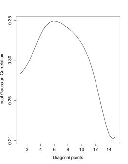
Figure 7: The estimated local Gaussian correlation between the IBM and Coca-Cola transaction data on a diagonal grid.

References

• Ahmad (2016) Ahmad, A. (2016). Contributions à l’éconemétrie des séries temporelles à valeurs entières. Ph. D. thesis, University Charles De Gaulle-Lille III, France.
• Ahmad and Franq (2016) Ahmad, A. and C. Franq (2016). Poisson QMLE of count time series models. Journal of Time Series Analysis 37, 291–314.
• Andreassen (2013) Andreassen, C. M. (2013). Models and inference for correlated count data. Ph. D. thesis, Aaarhus University, Denmark.
• Andrews (1984) Andrews, D. (1984). Non-strong mixing autoregressive processes. Journal of Applied Probability 21, 930–934.
• Basawa and Prakasa Rao (1980) Basawa, I. V. and R. L. S. Prakasa Rao (1980). Statistical Inference for Stochastic Processes. London: Academic Press.
• Berentsen et al. (2014) Berentsen, G. D., B. Støve, D. Tjøstheim, and T. Nordbø (2014). Recognizing and visualizing copulas: an approach using local Gaussian approximation. Insurance: Mathematics & Economics 57, 90–103.
• Bollerslev (1986) Bollerslev, T. (1986). Generalized autoregressive conditional heteroskedasticity. Journal of Econometrics 31, 307–327.
• Boudreault and Charpentier (2011) Boudreault, M. and A. Charpentier (2011). Multivariate integer-valued autoregressive models applied to earthquake counts. Technical report. available at http://arxiv.org/abs/1112.0929.
• Brockwell and Davis (1991) Brockwell, P. J. and R. A. Davis (1991). Time Series: Data Analysis and Theory (2nd ed.). New York: Springer.
• Chow (1967) Chow, Y. S. (1967). On a strong law of large numbers for martingales. Ann. Math. Statist. 38, 610.
• Christou and Fokianos (2014) Christou, V. and K. Fokianos (2014). Quasi-likelihood inference for negative binomial time series models. Journal of Time Series Analysis 35, 55–78.
• Cox (1981) Cox, D. R. (1981). Statistical analysis of time series: Some recent developments. Scandinavian Journal of Statistics 8, 93–115.
• Davis et al. (2000) Davis, R. A., W. T. M. Dunsmuir, and Y. Wang (2000). On autocorrelation in a Poisson regression model. Biometrika 87, 491–505.
• Davis and Liu (2016) Davis, R. A. and H. Liu (2016). Theory and inference for a class of observation-driven models with application to time series of counts. Statistica Sinica 26, 1673–1707.
• Dedecker et al. (2007) Dedecker, J., P. Doukhan, G. Lang, J. R. León R., S. Louhichi, and C. Prieur (2007). Weak dependence: with examples and applications, Volume 190 of Lecture Notes in Statistics. New York: Springer.
• Douc et al. (2013) Douc, R., P. Doukhan, and E. Moulines (2013). Ergodicity of observation-driven time series models and consistency of the maximum likelihood estimator. Stochastic Processes and their Applications 123, 2620–2647.
• Doukhan et al. (2012a) Doukhan, P., K. Fokianos, and X. Li (2012a). On weak dependence conditions: The case of discrete valued processes. Statistics & Probability Letters 82, 1941 – 1948.
• Doukhan et al. (2012b) Doukhan, P., K. Fokianos, and D. Tjøstheim (2012b). On weak dependence conditions for Poisson autoregressions. Statistics & Probability Letters 82, 942–948. (with a correction note in 83, 1926 – 1927, (2013)).
• Doukhan and Louhichi (1999) Doukhan, P. and S. Louhichi (1999). A new weak dependence condition and applications to moment inequalities. Stochastic Processes and their Applications 84, 313–342.
• Doukhan and Wintenberger (2008) Doukhan, P. and O. Wintenberger (2008). Weakly dependent chains with infinite memory. Stochastic Processes and Their Applications 118, 1997–2013.
• Ferland et al. (2006) Ferland, R., A. Latour, and D. Oraichi (2006). Integer–valued GARCH processes. Journal of Time Series Analysis 27, 923–942.
• Fokianos (2015) Fokianos, K. (2015). Statistical Analysis of Count Time Series Models: A GLM perspective. In R. Davis, S. Holan, R. Lund, and N. Ravishanker (Eds.), Handbook of Discrete-Valued Time Series, Handbooks of Modern Statistical Methods, pp.  3–28. London: Chapman & Hall.
• Fokianos et al. (2009a) Fokianos, K., A. Rahbek, and D. Tjøstheim (2009a). Poisson autoregression. Journal of the American Statistical Association 104, 1430–1439.
• Fokianos et al. (2009b) Fokianos, K., A. Rahbek, and D. Tjøstheim (2009b). Poisson autoregression (complete vesrion). available at http://pubs.amstat.org/toc/jasa/104/488.
• Fokianos and Tjøstheim (2011) Fokianos, K. and D. Tjøstheim (2011). Log–linear Poisson autoregression. Journal of Multivariate Analysis 102, 563–578.
• Francq and Zakoï an (2016) Francq, C. and J.-M. Zakoï an (2016). Estimating multivariate volatility models equation by equation. J. R. Stat. Soc. Ser. B. Stat. Methodol. 78, 613–635.
• Francq and Zakoïan (2010) Francq, C. and J.-M. Zakoïan (2010). GARCH models: Stracture, Statistical Inference and Financial Applications. United Kingdom: Wiley.
• Franke and Rao (1995) Franke, J. and T. S. Rao (1995). Multivariate first-order integer values autoregressions. Technical report, Department of Mathematics, UMIST.
• Genest and Nešlehová (2007) Genest, C. and J. Nešlehová (2007). A primer on copulas for count data. Astin Bull. 37, 475–515.
• Hall and Heyde (1980) Hall, P. and C. C. Heyde (1980). Martingale Limit Theory and its Applications. New York: Academic Press.
• Heinen (2003) Heinen, A. (2003). Modelling time series count data: An autoregressive conditional poisson model. Technical Report MPRA Paper 8113, University Library of Munich, Germany. availabel at http://mpra.ub.uni-muenchen.de/8113/.
• Heinen and Rengifo (2007) Heinen, A. and E. Rengifo (2007). Multivariate autoregressive modeling of time series count data using copulas. Journal of Empirical Finance 14, 564 – 583.
• Heyde (1997) Heyde, C. C. (1997). Quasi-Likelihood and its Applications: A General Approach to Optimal Parameter Estimation. New York: Springer.
• Hjort and Jones (1996) Hjort, N. L. and M. C. Jones (1996). Locally parametric nonparametric density estimation. The Annals of Statistics 24, 1619–1647.
• Joe (1997) Joe, H. (1997). Multivariate Models and Dependence Concepts. London: Chapman & Hall.
• Johnson et al. (1997) Johnson, N. L., S. Kotz, and N. Balakrishnan (1997). Discrete multivariate distributions. John Wiley, New York.
• Jørgensen et al. (1996) Jørgensen, B., S. Lundbye-Christensen, P. X.-K. Song, and L. Sun (1996). State-space models for multivariate longitudinal data of mixed types. The Canadian Journal of Statistics 24, 385–402.
• Jung et al. (2011) Jung, R., R. Liesenfeld, and R. Jean-François (2011). Dynamic factor models for multivariate count data: an application to stock–market trading activity. Journal of Business & Economic Statistics 29, 73–85.
• Karlis (2016) Karlis, D. (2016). Modelling multivariate times series for counts. In R. Davis, S. Holan, R. Lund, and N. Ravishanker (Eds.), Handbook of Discrete-Valued Time Series, Handbooks of Modern Statistical Methods, pp.  407–424. London: Chapman & Hall.
• Klimko and Nelson (1978) Klimko, L. A. and P. I. Nelson (1978). On conditional least squares estimation for stochastic processes. The Annals of Statistics 6, 629–642.
• Latour (1997) Latour, A. (1997). The multivariate GINAR(p) process. Advances in Applied Probability 29, 228–248.
• Lee et al. (2017) Lee, Y., S. Lee, and D. Tjøstheim (2017). Asymptotic normality and parameter change test for bivariate poisson INGRCH models. submitted for publication.
• Liang and Zeger (1986) Liang, K.-Y. and S. L. Zeger (1986). Longitudinal data analysis using generalized linear models. Biometrika 73, 13–22.
• Liu (2012) Liu, H. (2012). Some models for time series of counts. Ph. D. thesis, Columbia University, USA.
• Lütkepohl (2005) Lütkepohl, H. (2005). New Introduction to Multiple Time Series Analysis. Berlin: Springer-Verlag.
• McCullagh and Nelder (1989) McCullagh, P. and J. A. Nelder (1989). Generalized Linear Models (2nd ed.). London: Chapman & Hall.
• Meyn and Tweedie (1993) Meyn, S. P. and R. L. Tweedie (1993). Markov Chains and Stochastic Stability. London: Springer.
• Neumann (2011) Neumann, M. (2011). Absolute regularity and ergodicity of Poisson count processes. Bernoulli 17, 1268–1284.
• Paul et al. (2008) Paul, M., L. Held, and A. M. Toschke (2008). Multivariate modelling of infectious disease surveillance data. Statistics in Medicine 27, 6250–6267.
• Pedeli and Karlis (2013a) Pedeli, X. and D. Karlis (2013a). On composite likelihood estimation of a multivariate INAR(1) model. Journal of Time Series Analysis 34, 206–220.
• Pedeli and Karlis (2013b) Pedeli, X. and D. Karlis (2013b). Some properties of multivariate INAR(1) processes. Computational Statistics & Data Analysis 67, 213 – 225.
• Ravishanker et al. (2014) Ravishanker, N., V. Serhiyenko, and M. R. Willig (2014). Hierarchical dynamic models for multivariate times series of counts. Statistics and its Interface 7, 559–570.
• Ravishanker et al. (2015) Ravishanker, N., R. Venkatesan, and S. Hu (2015). Dynamic models for time series of counts with a marketing application. In R. Davis, S. Holan, R. Lund, and N. Ravishanker (Eds.), Handbook of Discrete-Valued Time Series, Handbooks of Modern Statistical Methods, pp.  425–446. London: Chapman & Hall.
• Rosenblatt (1956) Rosenblatt, M. (1956). A central limit theorem and a strong mixing condition. Proceedings of the National Academy of Sciences USA 42, 43–47.
• Rydberg and Shephard (2000) Rydberg, T. H. and N. Shephard (2000). A modeling framework for the prices and times of trades on the New York stock exchange. In W. J. Fitzgerlad, R. L. Smith, A. T. Walden, and P. C. Young (Eds.), Nonlinear and Nonstationary Signal Processing, pp.  217–246. Cambridge: Isaac Newton Institute and Cambridge University Press.
• Seber (2008) Seber, G. A. F.  (2008). A Matrix Handbook for Statisticians Hoboken: Wiley.
• Støve et al. (2014) Støve, B., D. Tjøstheim, and K. Hufthammer (2014). Using local Gaussian correlation in a nonlinear re-examination of financial contagion. Journal of Empirical Finance 25, 62 – 82.
• Taniguchi and Kakizawa (2000) Taniguchi, M. and Y. Kakizawa (2000). Asymptotic theory of statistical inference for time series. New York: Springer.
• Teräsvirta et al. (2010) Teräsvirta, T., D. Tjøstheim, and C. W. J. Granger (2010). Modelling Nonlinear Economic Time Series. Oxford: Oxford University Press.
• Tjøstheim (2012) Tjøstheim, D. (2012). Some recent theory for autoregressive count time series. TEST 21, 413–438.
• Tjøstheim (2015) Tjøstheim, D. (2015). Count Time Series with Observation-Driven Autoregressive Parameter Dynamics. In R. Davis, S. Holan, R. Lund, and N. Ravishanker (Eds.), Handbook of Discrete-Valued Time Series, Handbooks of Modern Statistical Methods, pp.  77–100. London: Chapman & Hall.