Convolutional Neural Pyramid for Image Processing

Abstract

We propose a principled convolutional neural pyramid (CNP) framework for general low-level vision and image processing tasks. It is based on the essential finding that many applications require large receptive fields for structure understanding. But corresponding neural networks for regression either stack many layers or apply large kernels to achieve it, which is computationally very costly. Our pyramid structure can greatly enlarge the field while not sacrificing computation efficiency. Extra benefit includes adaptive network depth and progressive upsampling for quasi-realtime testing on VGA-size input. Our method profits a broad set of applications, such as depth/RGB image restoration, completion, noise/artifact removal, edge refinement, image filtering, image enhancement and colorization.

1 Introduction

Convolutional neural networks (CNNs) become the most powerful tool for high-level computer vision tasks, such as object detection [12], image classification [23] and semantic segmentation [28]. Along this line, CNNs were also used to solve image processing problems. Representative applications are image/video super-resolution [6, 7, 19, 18, 25], artifact and noise removal [5, 8, 30], completion/inpainting [33, 43], learning image filtering [46, 27], image deconvolution [45], etc.

Compared to very successful classification and detection, low-level-vision neural networks encounter quite different difficulties when they are adopted as regression tools.

Figure 1: Receptive field size vs. running time of current low-level-vision CNNs, including SRCNN [6], Filter-CNN [46], VDSR [18], Shepard-CNN [33] and Deconv-CNN [45]. Our network achieves a very large receptive field efficiently, which enables many general learning applications. Running time is obtained during testing on a Nvidia Titan X graphics card with VGA-size color-image input.

(a) Depth/RGB Restoration	(b) Image Completion	(c) Artifact/Noise Removal	(d) Learning Image Filter

Figure 2: Our convolutional neural pyramid benefits many image-level applications including depth/RGB image restoration, image completion, artifact/noise removal, and learning image filter.

Size of Receptive Field for Image Processing

The first problem is about the receptive field, which is the region in the input layer connected to an output neuron. A reasonably large receptive field can capture global information applied to inference. In VGG [40] and ResNet [14], a large receptive field is achieved mainly by stacking convolution and pooling layers. For low-level-vision CNNs [6, 45, 18, 46, 24, 7], the pooling layers are commonly removed in order to regress the same-resolution output and preserve image details. To still obtain acceptable receptive fields with the convolution layers, the two solutions are to use large kernels (e.g. $7\times 7$ or $9\times 9$) [6, 46, 24] and stack many layers [18].

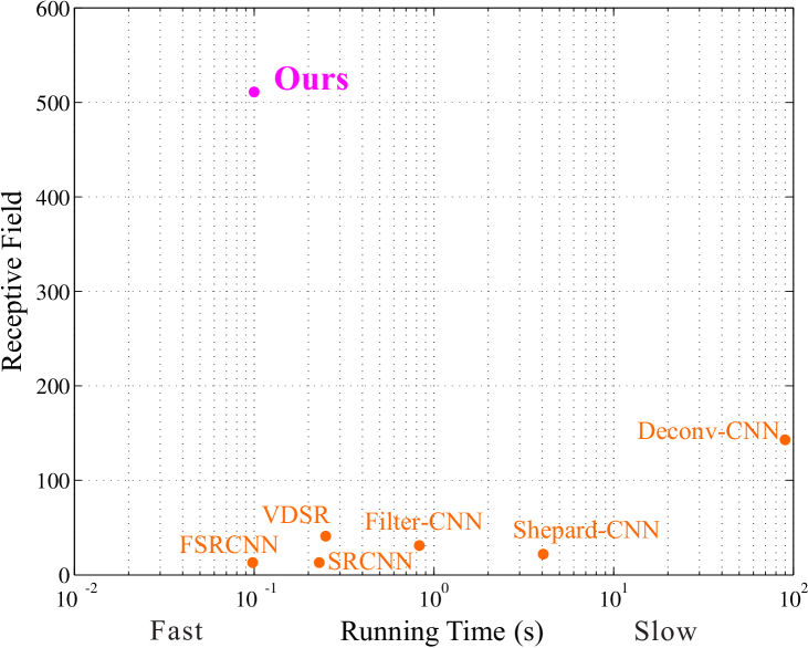
We found unexceptionally these two schemes both make the system run slowly due to heavy computation and consume a lot of memory. To illustrate it, we show the relation between the size of a receptive field and running time of current low-level-vision CNNs in Figure 1. It is observed based on this plot that most existing low-level-vision CNNs, such as SRCNN [6], Filter-CNN [46], VDSR [18], and Shepard-CNN [33], achieve receptive fields smaller than $41\times 41$ (pixels). Their applications are accordingly limited to local-information regression ones such as super-resolution, local filtering, and inpainting. On the other hand, Deconv-CNN [45] uses $143\times 143$ field size. But its computation cost is very high as shown in Figure 1.

Contrary to these common small receptive fields, our important finding is that large or even whole-image fields are essential for many low-level vision tasks because most of them, including image completion, restoration, colorization, matting, global filtering, are based on global-information optimization.

In this paper, we address this critical and general issue, and design a new network structure to achieve very-large receptive fields without sacrificing much computation efficiency, as illustrated in Figure 1.

Information Fusion

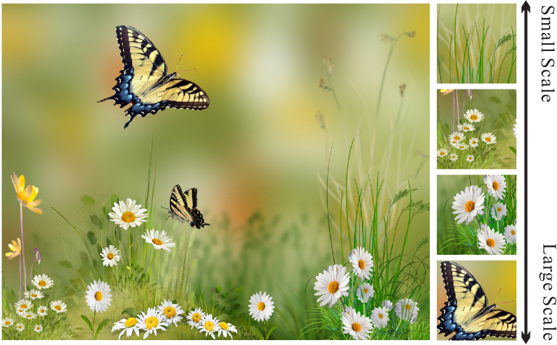
The second difficulty is on multiscale information fusion. It is well known that most image content is with multiscale patterns as shown in Figure 3. As discussed in [50], the small-scale information such as edge, texture and corners are learned in early layers and object-level knowledge comes from late ones in a deep neural network. This analysis also reveals the fact that color and edge information vanishes in late hidden layers. For pixel labeling work, such as semantic segmentation [28] and edge detection [27], early feature maps were extracted and taken into late layers to improve pixel inference accuracy.

We address this issue differently for low-level-vision tasks that do not involve pooling. Although it seems that the goal of retaining early-stage low-level edge information contradicts large receptive field generation in a deep network, our solution shows they can accomplished simultaneously with a general network structure.

Figure 3: Natural images contain different scales of details, texture, and objects.

Our Approach and Contribution

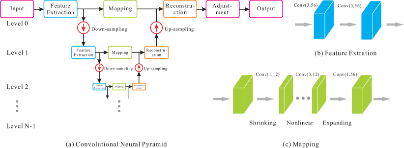
To address aforementioned difficulties, we propose convolutional neural pyramid (CNP), which can achieve quite large receptive fields while not losing efficiency as shown in Figure 1. It intriguingly enables multiscale information fusion for general image tasks. The convolutional neural pyramid structure is illustrated in Figure 4 where a cascade of features are learned in two streams. The first stream across different pyramid levels plays an important role for enlarging the receptive field. The second stream learns information in each pyramid level and finally merges it to produce the final result.

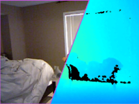
Our CNP benefits a wide spectrum of applications. As demonstrated in Figure 2, we achieve the state-of-the-art performance in depth/RGB restoration, image completion/inpainting, noise/artifact removal, etc. Other applications include learning image filter, image colorization, optical flow and stereo map refinement, image enhancement, and edge refinement. They are shown in the experiment section and our supplementary file.

Our framework is very efficient in computation. On an Nvidia Titan X display card, 28 frames are processed per second for a QVGA-size input and 9 frames per second for a VGA-size input for all image tasks.

Figure 4: Illustration of our convolutional neural pyramid. (a) shows the convolutional pyramid structure. (b) and (c) are the feature extraction and mapping components respectively. $Conv(x,y)$ denotes the convolution operation, where $x$ is the kernel size and $y$ is the number of output.

2 Related Work

We review recent progress of using CNNs for computational photography and low-level computer vision.

Inverse Problems

CNNs were used to solve inverse problems such as image super-resolution/upsampling and deconvolution. Representative methods include SRCNN [6], very-deep CNNs [18], deeply-recursive CNNs [19], and FSRCNN [7]. The major scheme is to regress the inverse degradation function by stacking many CNN layers, such as convolution and ReLU. They are mostly end-to-end frameworks. Image super-resolution frameworks were extended to video/multi-frame super-resolution [25] and depth upsampling [16]. All these frameworks are with relatively small receptive fields, which are hard to be extended to general image processing tasks.

Another important topic is image deconvolution, which needs image priors, such as gradient distribution, to constrain the solution. Xu et al. [45] demonstrated that simple CNNs can well approximate the inverse kernel and achieved decent results. As shown in Figure 1, large kernels for convolution require heavy computation.

Decomposition

Image decomposition applies filtering. Xu et al. learned general image filters of bilateral [42], rolling guidance [51], RTV [47], $L_{0}$ [44], etc. For learned recursive filter Liu et al. [27], image structure/edge information is inferred and fed into the recursive layers as weights. This framework is efficient. Deep joint image filtering [24] addresses the joint estimation problem.

Besides filtering, CNNs were also used for compression artifact removal [5], dirt/rain removal [8], denoising [43, 30], etc. Simply put, these frameworks employ CNNs to regress image structure. We show that our deep convolutional pyramid can better address global-optimization-like decomposition problems because of our large receptive fields with information fusion.

Image Completion/Inpainting

Considering sparse coding and CNNs, an auto-encoder framework for blind image inpainting was proposed in [43]. Köhler et al. [21] directly trained a CNN taking a specified mask and origin image as input. Ren et al. [33] enhanced the convolution layer to Shepard convolution. These methods also produce limited receptive fields. Recently, a semantic inpainting framework [48] incorporates perceptual and contextual loss. They achieved good results even with large holes for similar-content images.

Representative CNNs for High-level Tasks

Many CNNs are proposed for high-level recognition tasks. Famous ones include AlexNet [23], VGG [40], GoogleLeNet [41] and ResNet [15]. Based on these frameworks, lots of networks are proposed to solve semantic image segmentation as pixel classification. They include FCN [28], DeepLab [3], SegNet [1], U-Net [34] and those of [49, 26, 11, 31]. Compared with these image-to-label or image-to-label-map frameworks, our CNP aims for image processing directly by image-to-image regression.

3 Convolutional Neural Pyramid

To achieve large receptive fields, our convolutional neural pyramid network is illustrated in Figure 4. It includes levels from $0$ to $N-1$ as shown in Figure 4(a) where $N$ is the number of levels. We denote these levels as $L_{i}$ where $i\in\{0\cdot\cdot\cdot N-1\}$. Different-scale content is encoded in them. The feature extraction, mapping and reconstruction operations are denoted as $\mathcal{F}_{i}$, $\mathcal{M}_{i}$ and $\mathcal{R}_{i}$ respectively in each pyramid level. The input to $L_{i}$ is the feature extracted from $L_{i-1}$ after downsampling, essential to enlarge the receptive-field.

Specifically, the input to $L_{0}$ is the raw data, such as RGB channels. After feature extraction and mapping in each level, information is reconstructed from $L_{N-1}$ to $L_{0}$ where the output of each $L_{i}$ is upsampled and fused with the output from $L_{i-1}$. Thus scale-sensitive information is used together to reconstruct the final output.

3.1 Beyond Simple Multiscale Fusion

Before going to details for each component, we explain that our CNP is fundamentally different from and superior to the intuitive multiscale fusion strategy regarding the overall structure where the latter scheme processes each-scale input by feature extraction, mapping and reconstruction respectively and sums these outputs into the final result. There are two major differences in our network structure.

Adaptive Network Depth in Levels

First, in the original resolution, i.e., level 0 in Figure 4(a), only two convolution layers are performed for feature extraction. It is a shallow network that can well capture the edge and color information as previously discussed – its complexity is low.

Then in level 1, after downsampling to reduce feature map size, another feature extraction module is performed, which involves more convolution layers for deeper processing of the input image. It begins to extract more complicated patterns beyond edges due to its higher depth and accordingly larger receptive fields. The complexity is not much increased with the reduced feature map size.

When the network contains more levels, they are with even smaller feature maps processed more deeply to form semantically meaningful information regarding objects and shapes. The receptive fields are further increased while the computation complexity is caped to a reasonably small value. This adaptive depth strategy is remarkably effective in a lot of tasks. We will show experimental evaluation later.

Progressive Upsampling

During the final upsampling phase (after mapping) in Figure 4(a), directly upsampling the output from level $i$ to level $0$ needs a large kernel since the upsampling ratio is $2^{i}$, which makes learning difficult and possibly inaccurate. We address this issue by a progressive scheme from level $N-1$ to $0$. For each phase, the output in level $i$ is upsampled and then fused with the output in level $i-1$. Thus, the ratio is only 2 where $3\times 3$ efficient upsampling kernel suffices. Further, information in level $i-1$ is upsampled with the guidance from level $i$ since the upsampling kernel is learned between the two neighboring levels. It avoids possible edge and feature distortion when reconstructing the final result.

The empirical comparison with the simple multiscale fusion strategy will be provided after explaining all following components in our network.

3.2 Component Details

Feature Extraction

We apply convolution layers to extract image features. As shown in Figure 4(b), two convolution layers with PReLU rectification are employed for each feature extraction module. The low-level image features such as edges and corners can be extracted by one module [50] in level 0. Semantically more meaningful information is constructed with more extraction modules regarding our adaptive depth in other levels.

Each convolution layer outputs $56$ features with a $3\times 3$ kernel. For level 0, its feature output is a 56-channel map. Other levels take the input of feature extracted from another level after downsampling. Thus, $2*(i+1)$ convolution layers are applied to feature extraction in level $L_{i}$, where $i$ is the index, to learn complicated features. This pyramid design effectively enlarges the receptive field without quickly increasing computation. It also nicely encodes different-scale image information.

Mapping

The extracted features in each level $L_{i}$ are transformed by mapping $\mathcal{M}_{i}$. As demonstrated in Figure 4(c), our mapping includes shrinking, nonlinear transform and expanding blocks, motivated by the work of [7]. The shrinking layer embeds the 56-channel feature map into 12 channels by $1\times 1$ convolution. It reduces the feature dimension and benefits noise reduction.

The network is then stacked by nonlinear transform layers. Instead of applying large-kernel convolution [45, 6, 24] to achieve large receptive fields, we stack $S$ convolution layers with kernel size $3\times 3$ to reduce parameters and empirically achieve comparable performance. Since nonlinear transform is conducted in a low-dimension feature-space, computation efficiency is further improved. Here $S$ ranges from $1-3$. We will discuss its influence later.

Finally, an expanding layer is added to remap the 12-channel feature map into 56 channels by $1\times 1$ convolution, for reverse of the shrinking operation. We use this layer to gather more information to reconstruct high quality results.

Reconstruction

The reconstruction operation fuses information from two neighboring levels. For $L_{i}$ and $L_{i+1}$, the output of $L_{i+1}$ is upsampled and then fused with the output from $L_{i}$. The goal is to merge different-scale information progressively. We test two fusion operations of concatenating two outputs and element-wise sum of the outputs. They achieve comparable performance in our experiments. We thus use element-wise sum for a bit higher efficiency.

Down- and Up-sampling

Down- and up-sampling are key components in pyramid construction and collapse. The downsampling operation shown in Figure 4(a) resizes extracted feature maps. For simplicity, we only consider resizing ratio $0.5$ in our network. Two downsampling schemes are tested – max pooling and convolution with a $3\times 3$ kernel with stride $2$. The simple max pooling works better in experiments due to preservation of the max response. Note that in level $0$, our network does not include any pooling layer to keep image details. We simply implement the upsampling operation as a deconvolution layer in Caffe [17].

Adjustment

Since the reconstructed feature maps in $L_{0}$ are with 56 channels, to adjust difference between the feature map and output, we use two convolution layers with kernel size $3\times 3$ to generate the same number of channels as the final output, as shown in Figure 4(a). Before each convolution layer, a PReLU layer is applied.

Algorithm 1 gives the overall procedure, $\mathcal{F}_{i}(\mathbf{X})$ and $\mathcal{M}_{i}(\mathbf{X})$ are output of $\mathbf{X}$ after operations $\mathcal{F}_{i}$ and $\mathcal{M}_{i}$ respectively. $\mathcal{R}_{i}(\mathbf{X},\mathbf{X}_{1})$ is the reconstruction result of $\mathbf{X}$ and $\mathbf{X}_{1}$ with operation $\mathcal{R}_{i}$. Configuration of our network is provided in the supplementary file.

INPUT : $\mathbf{X}$

OUTPUT : $\mathbf{Y}$

/*Feature Extraction and Mapping*/ ;

$\mathbf{F}_{0}\leftarrow\mathcal{F}_{0}(\mathbf{X})$ ;

for t:= 1 to $N$  do

       $\mathbf{F}_{t}\leftarrow\mathcal{M}_{t}(\mathcal{F}_{t}(\downarrow\mathbf{F}_{t-1}))$  /*$\downarrow$ is down-sampling*/

$\mathbf{F}_{0}\leftarrow\mathcal{M}_{0}(\mathbf{F}_{0})$ ;

/*Reconstruction*/ ;

for t:= $N-1$ to $0$  do

       $\mathbf{F}_{t}\leftarrow\mathcal{R}_{t}(\mathbf{F}_{t},\uparrow\mathbf{F}_{t+1})$  /*$\uparrow$ is up-sampling*/

$\mathbf{Y}\leftarrow\mathbf{F}_{0}$ ;

Algorithm 1 Convolutional Neural Pyramid

3.3 More Analysis

The quite large receptive field, adaptive depth, and progressive fusion achieved by our CNP greatly improve performance for many tasks. We perform extensive evaluation and give the following analysis.

Receptive Field vs. Running Time  

In our $N$-level network, the information passing through level $L_{N-1}$ has the largest receptive field. For this level, the images are processed by feature extraction and downsampling for $N$ passes, which introduce a total of $2*N$ feature extraction operations. The receptive field size increases exponentially with the number of levels, making the largest receptive field $2^{N}$ times of the original one. Note that increasing the pyramid level introduces limited extra computation since the size of feature map decreases quickly in levels. The total extra computation for level ${N-1}$ is only $1/2^{N}$ of that in level $0$ for feature extraction.

The receptive field and running time statistics are reported in Table 1. For 5 levels, our testing time is only about 3 times of that spent in level 0 including overhead in up- and down-sampling. Note that there is only one feature extraction module in level 0 while level 4 has 5 of them. Our effective receptive field is as large as $511\times 511$ pixels.

We compare our CPN model with a baseline “Single-Level CNN” in Table 1 that does not contain any pyramid levels – so its structure is similar to level 0 of our model. In order to get $95\times 95$ receptive field, 48 $3\times 3$ convolution layers are needed, which consumes nearly 9GB GPU memory. Similar performance is yielded for our 3-level system.

	Our CPN			Single-Level CNN
Recept. Field	Levels	Time (s)	Mem. (GB)	Layers	Time (s)	Mem. (GB)
$15\times 15$	1	0.034	2.66	8	0.034	2.66
$39\times 39$	2	0.089	3.48	20	0.102	4.58
$95\times 95$	3	0.104	3.70	48	0.252	8.96
$223\times 223$	4	0.109	3.76	112	N/A	$>12$
$511\times 511$	5	0.111	3.77	256	N/A	$>12$

Table 1: Time and memory consumption analysis in terms of different sizes of receptive fields. “Single-Level CNN” denotes the baseline model without pyramid levels. VGA-size input images are used in experiments. Our GPU memory does not allow 112 or 256 layers.

Total Levels	Simple multiscale Fusion	Ours
$2$	34.41	34.66
$3$	36.83	36.94
$4$	37.09	37.99
$5$	38.41	39.36

Table 2: Comparison with simple multiscale fusion on NYU Depth V2 data [39]. PSNRs are reported for each setting.

	$\mathcal{S}=1$	$\mathcal{S}=2$	$\mathcal{S}=3$
$N=0$	32.07	32.31	32.67
$N=1$	34.31	34.66	35.01
$N=2$	36.71	36.94	37.09
$N=3$	37.75	37.99	38.01
$N=4$	38.98	39.36	39.42

Table 3: Effectiveness of our method. PSNRs are reported according to the numbers of pyramid levels ($N$) and nonlinear transform layers ($S$) on the dataset of [39].

Figure 5: Effectiveness of our convolution neural pyramid. (a) and (b) are the reference RGB image and corresponding degraded depth map. (c) is the ground truth depth. (d-h) show results of different pyramid levels.

Comparison with Simple Multiscale Fusion

We compare our framework with simple multiscale fusion described in Section 3.1 under the same parameter setting and report the results in Table 2 for depth/RGB image restoration on NYU Depth V2 benchmark [39]. Our framework outperforms this alternative under all levels. More pyramid levels yield larger improvement because we adapt network depth in levels while simple multiscale fusion does not.

Effectiveness of the Pyramid

We use the same depth/RGB restoration benchmark to verify the effectiveness of our network because this task needs large-region information in different scales to fill in holes and remove artifacts. More details of the task are included in Section 4. We evaluate our network under different setting and report the results in Table 3. They indicate involving several pyramid levels can greatly improve depth/RGB restoration quality since it benefits from afore discussed large receptive field sizes. We also test the influence of $\mathcal{S}$, which is the number of the nonlinear transform layers. Setting it to $1-3$ does not significantly change the result since the receptive field is not much influenced.

Visualizing What CNP Learns

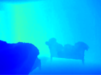
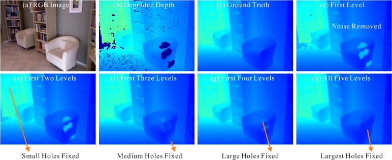
We visualize the information CNP learns regarding its different pyramid levels for depth restoration. We block some-level information to understand how it proceeds. The model is with $5$ levels and $1$ transform layer each. We first block levels $L_{1}-L_{4}$ and only show the result inferred from $L_{0}$ in Figure 5(d) – the small receptive field of $L_{0}$ is good to remove small holes. For large ones, artifacts are generated.

Then we gradually include more levels and show results in Figure 5(e-h). It is obvious that the capacity of removing holes increases as the total pyramid level expands. The biggest region on the chair is completely restored when all 5 levels are used. This manifests that these pyramid levels capture different degrees of semantic information. They work best on particular structure respectively. Our fusion process makes good use of all of them.

Relation to Previous Methods  

Traditional convolution pyramids [9] is only to approximate large-kernel convolution by a series of small ones. It is limited to gradient interpolation and does not extend to learning easily. Our network is obviously different due to the new structure and ability to learn general low-level vision operations.

When the number of our pyramid level is one, our network is similar to the network for image super-resolution [7]. We note our contribution is exactly on the pyramid structure and the effective adaptive depth for large receptive field generation. It can handle a large variety of complex tasks, which the method of [7] does not. We show these applications in what follows.

Difference from Detection and Segmentation CNNs  

Compared with popular CNNs such as VGG [40], ResNet [14] and FCN [28], the key difference is that our framework directly handles image-to-image regression for image processing in a very efficient way. Although some semantic segmentation frameworks, such as RefineNet [26], U-Net [34], and FRRN [31], also consider multi-scale information, they are fundamentally different due to the diverse nature of classification and regression. None of these methods can be directly applied (or through slight modification with regression loss) to our low-level vision tasks.

4 Experiments and Applications

We implement our network in Caffe [17] - training and testing are on a single NVIDIA Titan X graphics card. For most applications, we set $N=5$ and $\mathcal{S}=1$ by default. Following [18], we perform residual learning for all tasks. During training, $81\times 81$ patch size and $32$ batch size are applied. We use learning rate $10^{-5}$ for all model training. In general, training with 2 to 8 epoches is enough.

We set the training loss as the combination of $L_{2}$ loss in intensity and gradient. The reason is that intensity loss retains appearance while the gradient loss has the ability to keep results sharp. The loss is expressed as $\mathcal{L}(X,\hat{X})=\|X-\hat{X}\|+\lambda\|\nabla X-\nabla\hat{X}\|$, where $X$ is the prediction and $\hat{X}$ is the ground truth. $\nabla$ is the gradient operator and $\|\cdot\|$ computes the $L_{2}$ norm distance. $\lambda$ is the parameter balancing the two losses, set to $1$ in all experiments. Our framework can also use other loss functions, such as the generative loss. Exploring them will be our future work.

Figure 6: Comparison of depth/RGB restoration results. The images are from NYU Depth V2 dataset [39]. (a) and (b) are the RGB reference image and degraded depth respectively. (c) is the ground truth. (d-g) are results of bilateral filter [42], guided image filter [13], weighted median filter [52] and mutual-structure filtering [38] respectively. (h) is ours.

Depth/RGB Image Restoration   Depth map restoration with guidance of RGB images is an important task since depth captured by cameras such as Microsoft Kinect, is often with holes and severe noise. Depth estimated by stereo matching also contains errors in textureless and occlusion regions. Refining the produced depth is therefore needed for 3D reconstruction and geometry estimation. Our framework can address this problem.

We evaluate our method on NYU Depth V2 dataset [39], where depth is captured by Microsoft Kinect. It includes 1,449 aligned depth/RGB pairs. In our experiment, we treat the provided processed depth maps as ground truth and randomly select 10% image pairs for testing and the remaining 90% for training. We simply stack the gray-scaled RGB image, depth map, and the mask that indicates location of missing values as the input to the network. The output is the refined depth map.

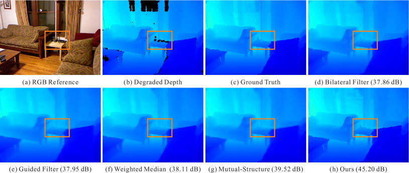
Comparison of different methods is reported in Table 4. For bilateral filter [42], guided image filtering [13], and weighted median filter [52], we first fill in the holes using joint-bilateral-filter-based normalized convolution [20] and then apply the filters to refine depth. We implement the method of [29] given no public code. The lower PSNRs by filter-based methods in Table 4 are due to big holes. Methods of Lu et al. [29] and mutual-structure filtering [38] achieve better results; but they face similar difficulties to restore large regions. our method produces high-quality results by properly handling different-scale holes.

We also evaluate our framework on the synthetic dataset [29]. Since there is no training data provided, we collect it from Middleburry stereo 2014 dataset [36] and MPI Sintel stereo dataset [2]. We degrade depth maps by adding holes and noise according to the method of [29]. Our model setting and training are the same as those on NYU Depth V2 dataset. The results are listed in Table 4 where all methods achieve good performance. It is because the synthetic data is simple. On the one hand, the reference image is with high quality. On the other hand, holes are relatively small.

In the visual comparison in Figure 6, our result is with sharp boundaries and many details. More results are provided in our supplementary file.

Methods	NYU Depth V2 Data	Lu et al. Data
Bilateral Filter [42]	26.19	34.33
Guided Filter [13]	27.02	34.86
Weighted Median[52]	31.19	38.17
Lu et al. [29]	34.53	39.20
Mutual-Structure [38]	33.97	39.13
Ours	39.42	39.21

Table 4: Comparisons of different depth/RGB restoration methods on the NYU Depth V2 and Lu et al. [29] datasets. We report average PSNRs of each method on the testing dataset.

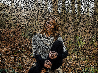
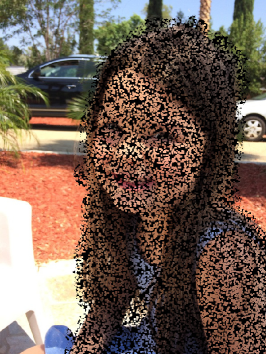
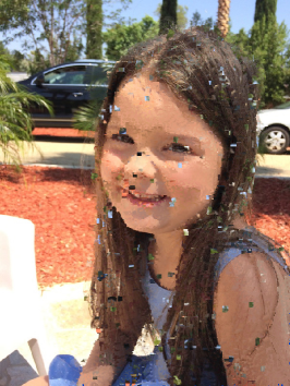
Natural Image Completion   We apply our method to image completion. For evaluation, we use the portrait dataset [37] since the portraits are with rich structure and details. For each portrait, we randomly set 5% pixels visible and dilate these visible regions by $4$ pixels. A degraded image is shown as Figure 7(a). The input to our framework is the degraded color image. We train our model with 1,800 portraits from [37] with our degradation. One example is shown in Figure 7 where (a) is the input. In Figure 7(b), the result of normalized convolution with bilateral filter [20] is a bit burry. The result in (c) is our trained model of [33] using our data. This method has difficulty to complete large holes because of the limited-size receptive field. PatchMatch-based method [22] produces result (d). Our result in (e) is a well restored image. The quantitative evaluation using the testing dataset from [37] with our degradation in Table 5 also manifests our superior performance.

(a) Input	(b) Result of [20]	(c) Result of [33]
(d) Result of [22]	(e) Ours	(f) Ground Truth

Figure 7: Comparisons of image completion results. (a) is the input. (b-d) are results of [20, 33, 22]. (e) is ours and (f) is the ground truth.

Methods	PSNRs
Normalized Convolution [20]	16.05
CNNs-based Inpaiting [33]	30.52
PatchMatch based Completion [22]	24.81
Ours	41.21

Table 5: Evaluation of image completion results on our dataset.

Learning Image Filter   Our framework also benefits image filter learning. Similar to those of [46] and [27], we use our deep convolution pyramid to learn common edge-preserving image filters, including weighted least square filter (WLS) [10], $L_{0}$ [44], RTV [47], weighted median filter (WMF) [52], and rolling guidance filter (RGF) [51]. These filters are representative ones with either global optimization or local computation. We employ the images from Imagenet [35] to train our models. The input to our network is color channels and the output is filtered color images. We quantitatively evaluate our method and previous approaches [46, 27] on the testing dataset of [46] by measuring PSNRs. As reported in Table 6, our framework outperforms that of [46] and achieves comparable performance to state-of-the-art method [27]. It is noteworthy that our testing is 31% faster than that of [27] on the same hardware.

Filter Type	PSNRs of [46]	PSNRs of [27]	Our PSNRs
WLS [10]	36.2	39.4	39.6
$L_{0}$ [44]	32.8	30.9	32.6
RTV [47]	32.1	37.1	38.0
WMF [52]	31.6	34.0	39.3
RGF [51]	35.9	42.2	42.6

Table 6: Performance of our framework for learning image filters. PSNRs of [46] and [27] are cited from paper [27].

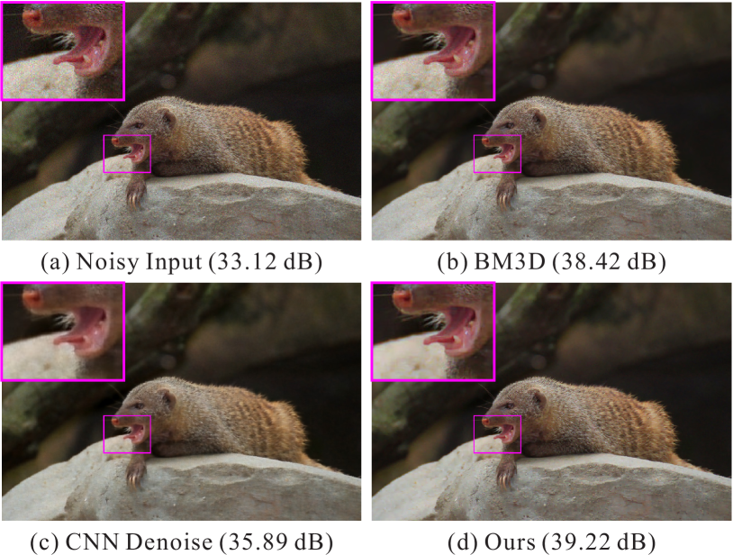
Image Noise Removal   Our framework can also be applied to image noise removal. We train our model on Imagenet data [35]. To get the noisy input close to real scenes we add Possion noise and Guassian white noise with deviation 0.01 to each image. Our model is directly trained on color images. One example is shown in Figure 8. Compared with previous BM3D [4] and CNN denoising [32] approaches shown in (b) and (c), our result contains less noise and well preserved details.

Figure 8: Comparison of image noise removal. (a) is the noisy input. (b) and (c) are the results of BM3D [4] and CNN based denoising [32] respectively. (d) is ours.

Other Applications   The powerful learning ability of our framework also benefits other image processing applications of learning image deconvolution, image colorization, image enhancement, edge refinement etc. More results are provided in our supplementary file.

5 Concluding Remarks

We have proposed a general and efficient convolution neutral network for low-level vision image processing tasks. It can produce very large receptive fields essential for many applications while not accordingly increase computation complexity. Our method is based on pyramid-style learning while introducing new adaptive depth mechanism. We have provided many examples to verify its effectiveness.

References

- [1] V. Badrinarayanan, A. Handa, and R. Cipolla. Segnet: A deep convolutional encoder-decoder architecture for robust semantic pixel-wise labelling. CoRR, abs/1505.07293, 2015.
- [2] D. J. Butler, J. Wulff, G. B. Stanley, and M. J. Black. A naturalistic open source movie for optical flow evaluation. In ECCV, pages 611–625, 2012.
- [3] L. Chen, G. Papandreou, I. Kokkinos, K. Murphy, and A. L. Yuille. Deeplab: Semantic image segmentation with deep convolutional nets, atrous convolution, and fully connected crfs. CoRR, abs/1606.00915, 2016.
- [4] K. Dabov, A. Foi, V. Katkovnik, and K. Egiazarian. Image denoising by sparse 3d transform-domain collaborative ltering. IEEE Transactions on Image Processing, 16(8), 2007.
- [5] C. Dong, Y. Deng, C. C. Loy, and X. Tang. Compression artifacts reduction by a deep convolutional network. In ICCV, pages 576–584, 2015.
- [6] C. Dong, C. C. Loy, K. He, and X. Tang. Image super-resolution using deep convolutional networks. IEEE Trans. Pattern Anal. Mach. Intell., 38(2):295–307, 2016.
- [7] C. Dong, C. C. Loy, and X. Tang. Accelerating the super-resolution convolutional neural network. In ECCV, pages 391–407, 2016.
- [8] D. Eigen, D. Krishnan, and R. Fergus. Restoring an image taken through a window covered with dirt or rain. In ICCV, pages 633–640, 2013.
- [9] Z. Farbman, R. Fattal, and D. Lischinski. Convolution pyramids. Proceedings of ACM SIGGRAPH, 30(6):175, 2011.
- [10] Z. Farbman, R. Fattal, D. Lischinski, and R. Szeliski. Edge-preserving decompositions for multi-scale tone and detail manipulation. ACM Trans. Graph., 27(3), 2008.
- [11] G. Ghiasi and C. C. Fowlkes. Laplacian pyramid reconstruction and refinement for semantic segmentation. In ECCV, pages 519–534, 2016.
- [12] R. B. Girshick. Fast R-CNN. In ICCV, pages 1440–1448, 2015.
- [13] K. He, J. Sun, and X. Tang. Guided image filtering. In ECCV, pages 1–14, 2010.
- [14] K. He, X. Zhang, S. Ren, and J. Sun. Deep residual learning for image recognition. CoRR, abs/1512.03385, 2015.
- [15] K. He, X. Zhang, S. Ren, and J. Sun. Deep residual learning for image recognition. In 2016 IEEE Conference on Computer Vision and Pattern Recognition, CVPR 2016, Las Vegas, NV, USA, June 27-30, 2016, pages 770–778, 2016.
- [16] T. Hui, C. C. Loy, and X. Tang. Depth map super-resolution by deep multi-scale guidance. In ECCV, pages 353–369, 2016.
- [17] Y. Jia, E. Shelhamer, J. Donahue, S. Karayev, J. Long, R. B. Girshick, S. Guadarrama, and T. Darrell. Caffe: Convolutional architecture for fast feature embedding. CoRR, abs/1408.5093, 2014.
- [18] J. Kim, J. K. Lee, and K. M. Lee. Accurate image super-resolution using very deep convolutional networks. CoRR, abs/1511.04587, 2015.
- [19] J. Kim, J. K. Lee, and K. M. Lee. Deeply-recursive convolutional network for image super-resolution. CoRR, abs/1511.04491, 2015.
- [20] H. Knutsson and C. Westin. Normalized and differential convolution. In CVPR, pages 515–523, 1993.
- [21] R. Köhler, C. J. Schuler, B. Schölkopf, and S. Harmeling. Mask-specific inpainting with deep neural networks. In GCPR, pages 523–534, 2014.
- [22] S. Korman and S. Avidan. Coherency sensitive hashing. In ICCV, pages 1607–1614, 2011.
- [23] A. Krizhevsky, I. Sutskever, and G. E. Hinton. Imagenet classification with deep convolutional neural networks. In NIPS, pages 1106–1114, 2012.
- [24] Y. Li, J. Huang, N. Ahuja, and M. Yang. Deep joint image filtering. In ECCV, pages 154–169, 2016.
- [25] R. Liao, X. Tao, R. Li, Z. Ma, and J. Jia. Video super-resolution via deep draft-ensemble learning. In ICCV, pages 531–539, 2015.
- [26] G. Lin, A. Milan, C. Shen, and I. D. Reid. Refinenet: Multi-path refinement networks for high-resolution semantic segmentation. CoRR, abs/1611.06612, 2016.
- [27] S. Liu, J. Pan, and M. Yang. Learning recursive filters for low-level vision via a hybrid neural network. In ECCV, pages 560–576, 2016.
- [28] J. Long, E. Shelhamer, and T. Darrell. Fully convolutional networks for semantic segmentation. In CVPR, pages 3431–3440, 2015.
- [29] S. Lu, X. Ren, and F. Liu. Depth enhancement via low-rank matrix completion. In CVPR, pages 3390–3397, 2014.
- [30] X. Mao, C. Shen, and Y. Yang. Image restoration using convolutional auto-encoders with symmetric skip connections. CoRR, abs/1606.08921, 2016.
- [31] T. Pohlen, A. Hermans, M. Mathias, and B. Leibe. Full-resolution residual networks for semantic segmentation in street scenes. CoRR, abs/1611.08323, 2016.
- [32] J. S. J. Ren and L. Xu. On vectorization of deep convolutional neural networks for vision tasks. In AAAI, pages 1840–1846, 2015.
- [33] J. S. J. Ren, L. Xu, Q. Yan, and W. Sun. Shepard convolutional neural networks. In NIPS, pages 901–909, 2015.
- [34] O. Ronneberger, P. Fischer, and T. Brox. U-net: Convolutional networks for biomedical image segmentation. In MICCAI, pages 234–241, 2015.
- [35] O. Russakovsky, J. Deng, H. Su, J. Krause, S. Satheesh, S. Ma, Z. Huang, A. Karpathy, A. Khosla, M. S. Bernstein, A. C. Berg, and F. Li. Imagenet large scale visual recognition challenge. International Journal on Computer Vision, 115(3):211–252, 2015.
- [36] D. Scharstein and R. Szeliski. A taxonomy and evaluation of dense two-frame stereo correspondence algorithms. International Journal on Computer Vision, 47(1-3):7–42, 2002.
- [37] X. Shen, X. Tao, H. Gao, C. Zhou, and J. Jia. Deep automatic portrait matting. In ECCV, pages 92–107, 2016.
- [38] X. Shen, C. Zhou, L. Xu, and J. Jia. Mutual-structure for joint filtering. In ICCV, pages 3406–3414, 2015.
- [39] N. Silberman, D. Hoiem, P. Kohli, and R. Fergus. Indoor segmentation and support inference from RGBD images. In ECCV, pages 746–760, 2012.
- [40] K. Simonyan and A. Zisserman. Very deep convolutional networks for large-scale image recognition. CoRR, abs/1409.1556, 2014.
- [41] C. Szegedy, W. Liu, Y. Jia, P. Sermanet, S. E. Reed, D. Anguelov, D. Erhan, V. Vanhoucke, and A. Rabinovich. Going deeper with convolutions. In CVPR, pages 1–9, 2015.
- [42] C. Tomasi and R. Manduchi. Bilateral filtering for gray and color images. In ICCV, pages 839–846, 1998.
- [43] J. Xie, L. Xu, and E. Chen. Image denoising and inpainting with deep neural networks. In NIPS, pages 350–358, 2012.
- [44] L. Xu, C. Lu, Y. Xu, and J. Jia. Image smoothing via L gradient minimization. ACM Trans. Graph., 30(6):174, 2011.
- [45] L. Xu, J. S. J. Ren, C. Liu, and J. Jia. Deep convolutional neural network for image deconvolution. In NIPS, pages 1790–1798, 2014.
- [46] L. Xu, J. S. J. Ren, Q. Yan, R. Liao, and J. Jia. Deep edge-aware filters. In ICML, pages 1669–1678, 2015.
- [47] L. Xu, Q. Yan, Y. Xia, and J. Jia. Structure extraction from texture via relative total variation. ACM Trans. Graph., 31(6):139, 2012.
- [48] R. Yeh, C. Chen, T. Lim, M. Hasegawa-Johnson, and M. N. Do. Semantic image inpainting with perceptual and contextual losses. CoRR, abs/1607.07539, 2016.
- [49] F. Yu and V. Koltun. Multi-scale context aggregation by dilated convolutions. CoRR, abs/1511.07122, 2015.
- [50] M. D. Zeiler and R. Fergus. Visualizing and understanding convolutional networks. In ECCV, pages 818–833, 2014.
- [51] Q. Zhang, X. Shen, L. Xu, and J. Jia. Rolling guidance filter. In ECCV, pages 815–830, 2014.
- [52] Q. Zhang, L. Xu, and J. Jia. 100+ times faster weighted median filter (WMF). In CVPR, pages 2830–2837, 2014.