Mass-size scaling $M\sim r^{1.67}$ of massive star-forming clumps – evidences of turbulence-regulated gravitational collapse

Abstract

We study the fragmentation of eight massive clumps using data from ATLASGAL 870 $\mu$m, SCUBA 850 and 450 $\mu$m, PdBI 1.3 and 3.5 mm, and probe the fragmentation from 1 pc to 0.01 pc scale. We find that the masses and the sizes of our objects follow $M\sim r^{1.68\pm 0.05}$. The results are in agreements with the predictions of Li (2017) where $M\sim r^{5/3}$. Inside each object, the densest structures seem to be centrally condensed, with $\rho(r)\sim r^{-2}$. Our observational results support a scenario where molecular gas in the Milky Way is supported by a turbulence characterized by a constant energy dissipation rate, and gas fragments like clumps and cores are structures which are massive enough to be dynamically detached from the ambient medium.

1 Introduction

Star formation is a fundamental process in the Milky Way and other galaxies. The star-forming regions exhibit structures over multiple scales, and they are believed to be primarily shaped by the interplay between turbulence and gravity (Mac Low & Klessen, 2004; Krumholz & McKee, 2005; Krumholz & Tan, 2007). Many diagnostics have been developed to quantify the properties of star-forming regions, which enable one to compare models with observations. These include the surface density probability density distribution (PDF) (Kainulainen et al., 2009; Kritsuk et al., 2011; Federrath, 2013; Vázquez-Semadeni & García, 2001), the correlation function (Padoan et al., 2009; Brunt et al., 2009; Rosolowsky et al., 1999), as well as the gravitational energy spectrum (Li & Burkert, 2016, 2017) which quantifies the multi-scale distribution of gravitational energy.

Comparing masses and sizes is a straightforward way to study the properties of the dense gas fragments. Previously, various mass-size relations have been proposed in the literature. Perhaps the most well-recognised one is the $M\sim r^{1.33}$ scaling by Kauffmann & Pillai (2010) as a threshold condition for regions to form massive protostars. In this paper, we compare the properties of sub-millimetre bright gas fragments in the mass-size plane. We are interested in sub-parsec scale structures that belong to the dense parts of the molecular interstellar medium (ISM), and the majority of them should collapse monotonically to form stars and star clusters.

Although the $M\sim r^{1.33}$ scaling by Kauffmann & Pillai (2010) has been widely used to interpret observations, it does not offer a description to the properties of the observed gas fragments. In fact, the observed dense gas fragments seem to follow a scaling relation with a steeper slope (Urquhart et al., 2014; Zhang et al., 2016; Gong et al., 2016). Recently, it has been suggested by Pfalzner et al. (2016) that both the cluster-forming clumps (Urquhart et al., 2014; Wienen et al., 2015) and the embedded star clusters (Lada & Lada, 2003) obey $M\sim r^{1.67}$. Li (2017) interprets this scaling as a result of gravitational collapse regulated by ambient turbulence. Although somewhat different scaling exponents have been reported in the literature, most of the clumps follow a relation that is steeper than $M\sim r^{1.33}$ and is close to $M\sim r^{1.67}$.

Due to limited resolution, previous analyses of the mass-size relation of the gas fragments focus on parsec-scale structures. On the other hand, according to Li (2017), properties of the dense gas fragments are determined by the interplay between turbulence and gravity over multiple scales, so it is natural to expect the mass-size relation $M\sim r^{1.67}$ to extend down to smaller scales. In this paper, we study the properties of gas fragments in star-forming regions by combining new observations with literature data. The observations were carried out with the Plateau de Bure Interferometer (PDBI) observational results with a criterion for quasi-isolated gravitational collapse derived in Li (2017).

2 Observations and data reduction

2.1 ATLASGAL clumps

The eight massive precluster clumps (G18.17, G18.21, G23.97N, G23.98, G23.44, G23.97S, G25.38, and G25.71) were selected from the SCUBA Massive Pre/Protocluster core Survey (SCAMPS; Thompson et al., 2005). These massive clumps have been covered by the Atacama Pathfinder Experiment (APEX) Telescope Large Area Survey of the Galaxy (ATLASGAL; Schuller et al., 2009). The survey was carried out at 870 $\mu$m with a beam size of 19.2^′′ with a rms in the range 40 to 60 ${\rm mJy~{}beam}^{-1}$, and had the goal of studying cold clumps associated with high-mass star-forming regions.

2.2 SCUBA clumps

The eight clumps were observed by the Submillimetre Common-User Bolometer Array (SCUBA) survey at 850 and 450 $\mu$m with James Clerk Maxwell Telescope (JCMT; Holland et al., 2013; Chapin et al., 2013) . The resolutions at 850 $\mu$m and 450 $\mu$m are $14^{\prime\prime}$ and $8^{\prime\prime}$ with rms of 0.20 and 1.6 ${\rm Jy~{}beam}^{-1}$, respectively.

2.3 PdBI cores, and condensations

The eight sources were observed with the IRAM Plateau de Bure Interferometer (PdBI) at 3.5 and 1.3 mm simultaneously with CD (for all eight sources) and BCD (only for four dense sources G23.44, G23.97S, G25.38, and G25.71) configurations during 2004 and 2006. The 3.5 mm receivers were tuned to 86.086 GHz in single sideband (SSB) mode. The 1.3 mm receivers were tuned to 219.560 GHz in double side-band (DSB) mode. Both receivers used two 320 MHz wide backends for continuum observation. For calibrations, the quasar B1741-038 was used as phase calibrator, and the quasar 3C273 and the evolved star MWC 349 were used as flux calibrators.

The CLIC and MAPPING modules in IRAM software package GILDAS were used for the data calibration and cleaning. The primary (synthesis) beam is about 58.5^′′ ($4.2^{\prime\prime}\times 2.8^{\prime\prime}$) at 86.086 GHz (or 3.5 mm) of CD tracks with a sensitivity of about 0.30 ${\rm mJy~{}beam}^{-1}$, and about 23.0^′′ ($0.8^{\prime\prime}\times 0.6^{\prime\prime}$) at 219.560 GHz (or 1.3 mm) of BCD tracks with a sensitivity of about 0.65 ${\rm mJy~{}beam}^{-1}$, respectively. Details concerning the PdBI data will be presented in forthcoming paper (Zhang et al. 2017 in prep.).

3 Results

3.1 Source extraction

We adopt typical terminologies where clumps, dense cores, and condensations as structures of physical FWHM sizes of $\sim$1, $\sim$0.1, and $\sim$0.01 pc, respectively (Williams et al., 2000). The Gaussclumps (Stutzki & Guesten, 1990; Kramer et al., 1998; Csengeri et al., 2014) in the GILDAS software package was used to structures at different scales and wavelengths from our samples. The Gaussclumps fits 2-dimensional gaussians locally to the maximums of the input data cube. It then subtracts this fragment from the cube, creates a residual map, and continues with the maximum of this residual map. The procedure is repeated until a stop criterion is met, for instance when the maximum of the residual maps drops below a certain level. In this paper, fragments with peak intensity above 5$\sigma$ are considered as signals.

3.2 Clump mass estimation

It is assumed that the dust emission is optically thin and the-gas to-dust ratio is 100 (Young & Scoville, 1991). The dust temperature is estimated using NH₃ (1, 1) and (2, 2) rotational lines observed by the Very Large Array (Zhang et al. 2017 in prep.). The fragment masses are calculated using dust opacities 0.002 cm² g^-1 at 3.5 mm, 0.009 cm² g^-1 at 1.3 mm, and 0.0185 cm² g^-1 at 870 $\mu$m (Ossenkopf & Henning, 1994; Pillai et al., 2011). The total masses $M$ of the sources can be calculated using (Kauffmann et al., 2008)

$$\begin{aligned} \left(\frac{M}{\rm M_{\sun}}\right)=&0.12\left({\rm e}^{14.39\left(\frac{\lambda}{\rm mm}\right)^{-1}\left(\frac{T_{\rm dust}}{\rm K}\right)^{-1}}-1\right)\times&\\ &\left(\frac{\kappa_{\nu}}{\rm cm^{2}g^{-1}}\right)^{-1}\left(\frac{S_{\nu}}{\rm Jy}\right)\left(\frac{D}{\rm kpc}\right)^{2}\left(\frac{\lambda}{\rm mm}\right)^{3},&\end{aligned}$$ (1)

where $\lambda$ is the observational wavelength, $T_{\rm dust}$ is the dust temperature, $\kappa_{\nu}$ is the dust opacity, $S_{\nu}$ is the integrated flux, and $D$ is the distance to the Sun. The integrated flux at 3.5 mm may be contributed by both dust and free-free emissions which were distinguished using spectral energy distribution (SED) fitting to multi-wavelength continuum data (e.g. Zhang et al., 2014). The detailed procedure and results will be presented in Zhang et al. (2017 in prep.). The mass uncertainties are mainly contributed from the uncertainties of the dust temperature estimates.

3.3 The results of ATLASGAL, SCUBA, and PdBI observations

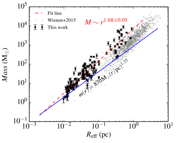
Figure 1: Mass-size plane for the eight sources (G18.17, G18.21, G23.97N, G23.98, G23.44, G23.97S, G25.38, and G25.71) at different wavelengths, together with the clumps from Wienen et al. (2015). The masses are derived from the integrated flux within a measured Gaussian $FWHM$ using the Gaussclumps, and the effective radii are defined as $R_{\rm eff}=FWHM/(2\sqrt{\rm ln2})$. The straight blue line shows a threshold to form high-mass protostars (Kauffmann & Pillai, 2010). The dashed red line shows the result of a power-law fit to the whole sample, where we find ${\rm log}(Mass(R_{\rm eff})/{\rm M_{\sun}})=3.85+1.68{\times}{\rm log}(R_{\rm eff}/{\rm pc})$ or $M\sim r^{1.68\pm 0.05}$ for short. It is comparable with the analytical result of Li (2017) where $M\sim r^{5/3}\sim r^{1.67}$.

In Figure 1 we plot the structures in the mass-size plane from 1 pc to 0.01 pc scale, by combining 870 $\mu$m, 850 $\mu$m, 450 $\mu$m, 3.5 mm, and 1.3 mm observational data (including data from G18.17, G18.21, G23.97N, G23.98, G23.44, G23.97S, G25.38, and G25.71). For comparison, we also plot the ATLASGAL clumps in Wienen et al. (2015). Our our sample sources are not included in their sample. The mass-size threshold $m(r)>870{\rm\rm M_{\sun}}(r/{\rm pc})^{1.33}$ for massive star formation (Kauffmann & Pillai, 2010) is also plotted for reference. A power-law fit to our data yields ${\log}(\rm Mass(R_{\rm eff})/{\rm M_{\sun}})=3.86+1.68{\times}{\rm log}(R_{\rm eff}/{\rm pc})$ or $(M/7000{\rm M_{\odot}})\approx(r/{\rm pc})^{1.68\pm 0.05}$ for short. The slope we obtained is similar to what was found in Urquhart et al. (2014) and Wienen et al. (2015). Our observations are selected to target at the most prominent fragments, which is probably the reason that the normalization mass-size scaling is higher than those presented in Urquhart et al. (2014) and Wienen et al. (2015).

In Figure 2 we plot the properties of the individual regions viewed in the mass-size plane. Different color-filled circles stand for the clumps and cores, respectively. We use dashed lines to connect the condensations with their host cores or clumps. Finally, we draw the thick green lines to connect the spatially overlapping objects that are most prominent at a given scale . These tree-diagrams enable us to represent the nested structure of a given clump. In some sense this is similar to a Dendrogram representation of the data (Rosolowsky et al., 2008).

We should note that the different observations have different spacial coverages: due to the limitation of the size of the primary beams of interferometer array, the 1.3 mm high-resolution observations cover only the central (23.0^′′) part of the region observed at 870 $\mu$m. We are only able to probe the fragmentation down to about 0.01 pc for four sources where the 1.3 mm high-resolution observations are available.

In Figure 3 we plot the distribution of the scaling exponents of all the pairs of nested structures. The red arrow points to the threshold condition $M\sim r^{1.67}$ (Li, 2017) for the model of turbulence-regulated gravitational collapse.

4 Discussion: Fragmentation in the mass-size plane

4.1 Gravitational collapse in a turbulent medium

Gravitational collapse in turbulent media has been intensively studied before. Earlier treatments such as Chandrasekhar (1951) and Parker (1952) assume constant velocity dispersions for the turbulent gas. In today’s view, their picture is probably over-simplified, as the multi-scaled structure of the turbulence flow is not well characterized. Subsequent works (Bonazzola et al., 1987; Vazquez-Semadeni & Gazol, 1995) describe the instability in a framework where they assume Kolmogorov-like power spectrum of turbulent energy and fractal-like density-size scalings. In particular, Vazquez-Semadeni & Gazol (1995) identified different regimes within which the interplay between turbulence and gravity produces different modes of collapse. The study revealed a diverse range of possibilities where gravitational collapse would occur. These results are interesting theoretically. However, a remaining difficulty is to study the non-linear outcome of the instability and to relate the structures they produced in the Fourier space with the dense gas fragments seen in observations. This task is highly non-trivial (Houlahan & Scalo, 1990).

Following previous studies, (Kauffmann et al., 2010; Ballesteros-Paredes et al., 2011a; Hennebelle, 2012; Lee & Hennebelle, 2016), Li (2017) considered the evolution of a dense object embedded in a diffuse medium, and study the interaction between the dense object and the ambient medium. They assume a picture where inside the object, gravity is driving contractions, and outside the object, turbulence is providing support. They carried out the analysis in the physical space, and studied the outcome of the interaction between the object and the ambient medium. Their main conclusion is that when the turbulence energy dissipation rate of the ambient medium is close to a constant, the objects that undergo gravitational collapse should follow the scaling relation $M\sim r^{1.67}$.

Note that the condition is independent on how objects are formed. It is certainly possible that the structures we see originate from a hierarchical, bottom-up assembly of smaller structures, as has been proposed by Ballesteros-Paredes et al. (2011a, b) and Vazquez-Semadeni et al. (2016). As long as the ambient have an almost-uniform level of turbulence, the scaling $M\sim r^{1.67}$ should hold.

4.2 $M\sim r^{1.67}$ as the threshold condition for gravitational collapse

We use the analytical prediction developed in Li (2017) to interpret our results. In their picture, the molecular ISM consists of two dynamical phases – a diffuse phase where turbulence dominates and a dense phase where gravity dominates. One major prediction of Li (2017) is that if the ambient turbulence is characterized by a constant energy dissipation rate $\epsilon$, gravitationally bound structures should obey $M\approx\epsilon^{2/3}\eta^{−2/3}G^{−1}r^{5/3}$ where $G$ is the gravitational constant and $r$ is the size. $\eta$ is a parameter for turbulent dissipation, and is close to unity. Thus the mass-size scaling is determined by the energy dissipation rate of the ambient medium $\epsilon$. When $\epsilon$ is a constant, $M\sim r^{5/3}$. This scaling has been supported by data from Pfalzner et al. (2016).

Gas condensations of smaller sizes were not studied in Pfalzner et al. (2016), because they are limited by the resolution of the single-dish continuum observations. However, the theoretical limit $M\sim r^{5/3}$ was derived by considering the interaction between gravity and an ambient turbulence, and one expects it to hold as long as turbulence can cascade effectively. In the molecular ISM, the limit of this cascade, namely the Kolmogorov microscale is very small ($10^{-6}$ pc as estimated in Fleck (1983)). Thus we expect this relation to be valid for structures on smaller scales.

With our new data we are probing structures down to $\sim 0.01\,\rm pc$ scale. Fig. 1 plots the mass-size plane from clump scale to $\sim 0.01\;\rm pc$ condensation scale, and a fit to the observational data suggests an universal mass-size relation ${\rm log}({\rm Mass}/{\rm M_{\sun}})=3.85+1.68{\times}{\rm log}(R_{\rm eff}/{\rm pc})$ (or $M\sim r^{1.68\pm 0.05}$ for short) that is valid from a few parsec to $\sim 0.01$ pc. Thus the scaling relation $M\sim r^{5/3}\sim r^{1.67}$ offers a good explanation to our multi-scale observational data. According to Li (2017), this is a direct consequence of the fact that the diffuse phase of the Milky Way ISM is dominated by a turbulence with a constant energy dissipation rate, and the observed structures are the dense parts that are dynamically detached from the ambient medium and are probably collapsing.

Other attempts have been made to explain the observed mass-size relation. It is straightforward to combine the Larson’s relation with the virial equilibrium to derive similar mass-size scalings. This has been previously attempted (Kauffmann et al., 2010; Ballesteros-Paredes et al., 2011a; Hennebelle, 2012; Lee & Hennebelle, 2016) . The derived scalings are somewhat similar to the one we observed. However, the interpretation of Li (2017) seems to be preferred over the previous ones for two reasons: first, the Larson relation has its own uncertainties; in the relation, the velocity dispersion $\sigma_{\rm v}$ and scale $l$ are related by $\sigma_{\rm v}\sim l^{\alpha}$ where the value of $\alpha$ is found to range from 1/3 to 1/2 (Larson, 1981; Heyer et al., 2009; Roman-Duval et al., 2011). If one simply derives the mass-size relation based on the Larson’s relation, assuming that the dense structures are gravitationally bound, using $M\sim\sigma_{\rm v}^{2}r/G$ one would predict a variety of mass-size scalings range from $M\sim r^{1.67}$ to $M\sim r^{2}$, and on the other hand, the observed scaling $M\sim r^{1.68\pm 0.05}$ stays very close to the $M\sim r^{1.67}$ prediction made by Li (2017). Second, it has been found that the clumps themselves do not obey the Larson’s relation (e.g. appendix A1 of Wienen et al., 2015). It is the ambient medium that satisfies the relation. Therefore, one should not directly combine the Larson’s relation with the gravitational bound argument to derive the mass-size relation. Realizing this, Li (2017) did not invoke the assumption that the dense structures are themselves following the Larson’s relation. Instead, they assume a constant energy dissipation rate in the ambient turbulence, and study the interaction between the object and the ambient turbulent medium. It is this interplay that determines the mass-size relation. In their picture, the ambient medium is dominated by turbulence, and follows the Larson’s relation. The objects are dynamically detached from the ambient medium, and they do not have to obey the relation.

4.3 Slopes in the mass-size plane

When an object is dynamically detached from the ambient medium, its evolution should be determined by the dynamics of the gravity-driven turbulence inside the object. Dedicated numerical simulations as well as analytical models have been developed to describe the collapse. When a region undergoes gravitational collapse, the density profile approaches $\rho\sim r^{-2}$ (Kritsuk et al., 2007; Federrath et al., 2010; Murray & Chang, 2015). However, one should note that this density profile can also be produced by gravitational free-fall (Girichidis et al., 2014) and magnetized models (Adams & Shu, 2007).

In observations, many of the star-forming regions seem to have $\rho\sim r^{-2}$. This should correspond to $M\sim r$. In Fig. 2 we plot the properties of different gas fragments in the mass-size plane, with connecting lines in the plot to denote structures that are spatially overlapping on the map. In Fig. 3 we present the distribution the slopes of these connecting lines in the mass-size plane. Since the high-resolution observations only cover the most central (23^′′) parts of the regions, we are essentially probing only the densest fragments. The massive connected fragments are much more centrally condensed than $M\sim r^{5/3}$ (31 of the connected structures out of 45 have slopes that are shallower than $M\sim r^{1.67}$) and seems to approach $\rho(r)\sim r^{-2}$, indicating that these structures are centrally-condensed enough to be dynamically detached from the ambient turbulence.

Using a technique called inverse dynamical population synthesis, Marks & Kroupa (2012) derived a mass-size relation $r/{\rm pc}\sim(M/M_{\odot})^{0.13\pm 0.04}$ for “cluster-forming cloud clumps”. Essentially, what they are constraining are the birthplaces of binary stars in star clusters. Their results indicate that the binaries in a star clusters are born within a very small radius (typically $\sim 0.1\;\rm pc$), and the scale is only weakly dependent on the mass. This perhaps suggests that the fragments we observed are still undergoing significant infall, and due to this transport, the stars are likely to be born at the very centres of the clumps. Although we can not explain this scaling analytically, it is at least consistent with our picture where gas inside the clumps is dynamically detached from the ambient turbulence and is collapsing.

5 Conclusions

In this work, we study the fragmentation of eight massive clumps using data from ATLASGAL 870 $\mu$m, PdBI 1.3 and 3.5 mm, and probed the fragmentation from 1 pc to 0.01 pc scale. Combined with previous measurements and analytical arguments, we propose a mass-size relation $M\sim r^{1.67}$ that holds from around 0.01 pc to 1 pc scale. The mass-size relation can be understood if the structures undergo quasi-isolated gravitational collapse in a turbulent medium, as predicted by Li (2017). The structures at the centres of the clumps are more centrally-condensed and seem to approach $M\sim r$ (which is equivalent to $\rho(r)\sim r^{-2}$).

Our observational results with $M\sim r^{1.68\pm 0.05}$ support a scenario where molecular gas in the Milky Way is supported by a turbulence with an almost constant energy dissipation rate, and gas fragments like clumps and cores are structures which are dense enough to be dynamically detached from the ambient medium.

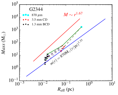
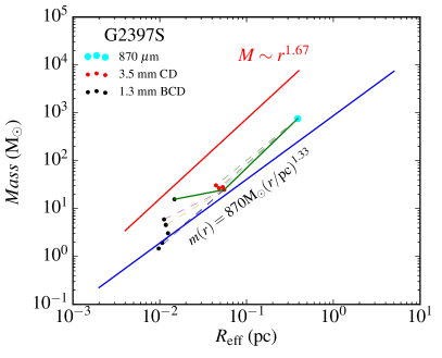
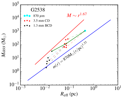
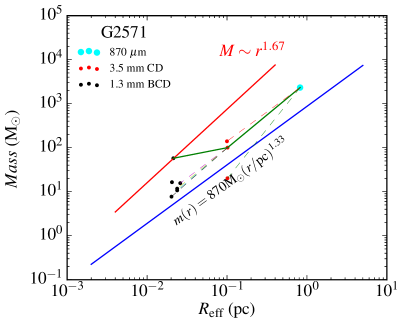
Figure 2: Fragmentation diagram of individual sources in the mass-size plane using data obtained at 870 $\mu$m, 3.5 mm CD track, and 1.3 mm BCD track. The masses are derived from the integrated flux within a measured Gaussian profile derived using the Gaussclumps, and the effective radius is $R_{\rm eff}=FWHM/(2\sqrt{\rm ln2})$. The straight blue lines show a threshold to form high-mass protostars (Kauffmann & Pillai, 2010). The thick green lines represent the set of structures within which the most prominent cores reside. The straight red line shows the scaling $M\sim r^{1.67}$ derived in Li (2017) as the threshold condition for gravitational collapse in a turbulent medium.

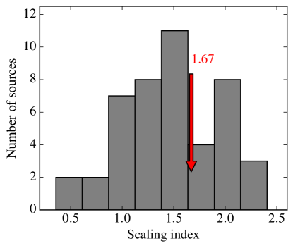
Figure 3: Histogram for the scaling index. The $x$-axis is the scaling index $k_{\rm m}$ of the mass-size relation ($M\sim r^{k_{\rm m}}$), the $y$-axis is the number of sources in each bin. A bin size of 0.26 dex is used. The distribution has a mean of 1.47, median of 1.48, and a standard deviation of 0.48. The red arrow points to the threshold condition $M\sim r^{1.67}$ for gravitational collapse derived in Li (2017).

References

- Adams & Shu (2007) Adams F. C., Shu F. H., 2007, ApJ, 671, 497
- Ballesteros-Paredes et al. (2011a) Ballesteros-Paredes J., Hartmann L. W., Vázquez-Semadeni E., Heitsch F., Zamora-Avilés M. A., 2011a, MNRAS, 411, 65
- Ballesteros-Paredes et al. (2011b) Ballesteros-Paredes J., Vázquez-Semadeni E., Gazol A., Hartmann L. W., Heitsch F., Colín P., 2011b, MNRAS, 416, 1436
- Bonazzola et al. (1987) Bonazzola S., Heyvaerts J., Falgarone E., Perault M., Puget J. L., 1987, A&A, 172, 293
- Brunt et al. (2009) Brunt C. M., Heyer M. H., Mac Low M.-M., 2009, A&A, 504, 883
- Chandrasekhar (1951) Chandrasekhar S., 1951, Proceedings of the Royal Society of London Series A, 210, 26
- Chapin et al. (2013) Chapin E. L., Berry D. S., Gibb A. G., Jenness T., Scott D., Tilanus R. P. J., Economou F., Holland W. S., 2013, MNRAS, 430, 2545
- Csengeri et al. (2014) Csengeri T., et al., 2014, A&A, 565, A75
- Federrath (2013) Federrath C., 2013, MNRAS, 436, 1245
- Federrath et al. (2010) Federrath C., Roman-Duval J., Klessen R. S., Schmidt W., Mac Low M.-M., 2010, A&A, 512, A81
- Fleck (1983) Fleck Jr. R. C., 1983, ApJ, 272, L45
- Girichidis et al. (2014) Girichidis P., Konstandin L., Whitworth A. P., Klessen R. S., 2014, ApJ, 781, 91
- Gong et al. (2016) Gong Y., et al., 2016, A&A, 588, A104
- Hennebelle (2012) Hennebelle P., 2012, A&A, 545, A147
- Heyer et al. (2009) Heyer M., Krawczyk C., Duval J., Jackson J. M., 2009, ApJ, 699, 1092
- Holland et al. (2013) Holland W. S., et al., 2013, MNRAS, 430, 2513
- Houlahan & Scalo (1990) Houlahan P., Scalo J., 1990, ApJS, 72, 133
- Kainulainen et al. (2009) Kainulainen J., Beuther H., Henning T., Plume R., 2009, A&A, 508, L35
- Kauffmann & Pillai (2010) Kauffmann J., Pillai T., 2010, ApJ, 723, L7
- Kauffmann et al. (2008) Kauffmann J., Bertoldi F., Bourke T. L., Evans II N. J., Lee C. W., 2008, A&A, 487, 993
- Kauffmann et al. (2010) Kauffmann J., Pillai T., Shetty R., Myers P. C., Goodman A. A., 2010, ApJ, 716, 433
- Kramer et al. (1998) Kramer C., Stutzki J., Rohrig R., Corneliussen U., 1998, A&A, 329, 249
- Kritsuk et al. (2007) Kritsuk A. G., Norman M. L., Padoan P., Wagner R., 2007, ApJ, 665, 416
- Kritsuk et al. (2011) Kritsuk A. G., Norman M. L., Wagner R., 2011, ApJ, 727, L20
- Krumholz & McKee (2005) Krumholz M. R., McKee C. F., 2005, ApJ, 630, 250
- Krumholz & Tan (2007) Krumholz M. R., Tan J. C., 2007, ApJ, 654, 304
- Lada & Lada (2003) Lada C. J., Lada E. A., 2003, ARA&A, 41, 57
- Larson (1981) Larson R. B., 1981, MNRAS, 194, 809
- Lee & Hennebelle (2016) Lee Y.-N., Hennebelle P., 2016, A&A, 591, A30
- Li (2017) Li G.-X., 2017, MNRAS, 465, 667
- Li & Burkert (2016) Li G.-X., Burkert A., 2016, MNRAS, 461, 3027
- Li & Burkert (2017) Li G.-X., Burkert A., 2017, MNRAS, 464, 4096
- Mac Low & Klessen (2004) Mac Low M.-M., Klessen R. S., 2004, Reviews of Modern Physics, 76, 125
- Marks & Kroupa (2012) Marks M., Kroupa P., 2012, A&A, 543, A8
- Murray & Chang (2015) Murray N., Chang P., 2015, ApJ, 804, 44
- Ossenkopf & Henning (1994) Ossenkopf V., Henning T., 1994, A&A, 291, 943
- Padoan et al. (2009) Padoan P., Juvela M., Kritsuk A., Norman M. L., 2009, ApJ, 707, L153
- Parker (1952) Parker E. N., 1952, Nature, 170, 1030
- Pfalzner et al. (2016) Pfalzner S., Kirk H., Sills A., Urquhart J. S., Kauffmann J., Kuhn M. A., Bhandare A., Menten K. M., 2016, A&A, 586, A68
- Pillai et al. (2011) Pillai T., Kauffmann J., Wyrowski F., Hatchell J., Gibb A. G., Thompson M. A., 2011, A&A, 530, A118
- Roman-Duval et al. (2011) Roman-Duval J., Federrath C., Brunt C., Heyer M., Jackson J., Klessen R. S., 2011, ApJ, 740, 120
- Rosolowsky et al. (1999) Rosolowsky E. W., Goodman A. A., Wilner D. J., Williams J. P., 1999, ApJ, 524, 887
- Rosolowsky et al. (2008) Rosolowsky E. W., Pineda J. E., Kauffmann J., Goodman A. A., 2008, ApJ, 679, 1338
- Schuller et al. (2009) Schuller F., et al., 2009, A&A, 504, 415
- Stutzki & Guesten (1990) Stutzki J., Guesten R., 1990, ApJ, 356, 513
- Thompson et al. (2005) Thompson M. A., Gibb A. G., Hatchell J. H., Wyrowski F., Pillai T., 2005, in Wilson A., ed., ESA Special Publication Vol. 577, ESA Special Publication. pp 425–426
- Urquhart et al. (2014) Urquhart J. S., et al., 2014, MNRAS, 443, 1555
- Vázquez-Semadeni & García (2001) Vázquez-Semadeni E., García N., 2001, ApJ, 557, 727
- Vazquez-Semadeni & Gazol (1995) Vazquez-Semadeni E., Gazol A., 1995, A&A, 303, 204
- Vazquez-Semadeni et al. (2016) Vazquez-Semadeni E., Gonzalez-Samaniego A., Colin P., 2016, preprint, (arXiv:1611.00088)
- Wienen et al. (2015) Wienen M., et al., 2015, A&A, 579, A91
- Williams et al. (2000) Williams J. P., Blitz L., McKee C. F., 2000, Protostars and Planets IV, p. 97
- Young & Scoville (1991) Young J. S., Scoville N. Z., 1991, ARA&A, 29, 581
- Zhang et al. (2014) Zhang C.-P., Wang J.-J., Xu J.-L., Wyrowski F., Menten K. M., 2014, ApJ, 784, 107
- Zhang et al. (2016) Zhang C.-P., et al., 2016, A&A, 585, A117