Winding in Non-Hermitian Systems

Abstract

This paper extends the property of interlacing of the zeros of eigenfunctions in Hermitian systems to the topological property of winding number in non-Hermitian systems. Just as the number of nodes of each eigenfunction in a self-adjoint Sturm-Liouville problem are well-ordered, so too are the winding numbers of each eigenfunction of Hermitian and of unbroken $\mathcal{PT}$-symmetric potentials. Varying a system back and forth past an exceptional point changes the windings of its eigenfunctions in a specific manner. Nonlinear, higher-dimensional, and general non-Hermitian systems also exhibit manifestations of these characteristics.

I Introduction

The first observations of optical systems with balanced gain and loss R1 ; R2 drew attention to $\mathcal{PT}$ symmetry R3 ; R4 . While the concept of $\mathcal{PT}$ symmetry originated in quantum mechanics and quantum field theory, the past decade has unearthed a trove of new experimental phenomena and potential applications of $\mathcal{PT}$ symmetry X1 ; X2 ; X3 ; X4 . The further discovery and understanding of these novel behaviors requires a fundamental comprehension of the underlying mathematical properties of $\mathcal{PT}$ systems. This paper investigates the inherent relationship between $\mathcal{PT}$ symmetry and the complex phase angle (to be defined) of an eigenfunction along a path in coordinate space.

The spectra of non-Hermitian Hamiltonians having an unbroken $\mathcal{PT}$ symmetry are entirely real R3 . Furthermore, there exists an inner product under which these Hamiltonians possess eigenfunctions with positive norms and exhibit unitary time evolution; thus they define physical quantum theories R4 . These properties of $\mathcal{PT}$-symmetric systems suggest the possibility that other hallmark features of Hermitian Hamiltonians might have analogues for $\mathcal{PT}$-symmetric Hamiltonians.

A characteristic property of a Hermitian Hamiltonian is the interlacing of the zeros of its eigenfunctions; that is, between any two consecutive nodes, or zeros, of an eigenfunction lies exactly one node of the next-higher-energy eigenfunction R5 . This relates directly to the completeness of the eigenfunctions. $\mathcal{PT}$-symmetric eigenfunctions also comprise a complete set R6 ; however, no $\mathcal{PT}$ counterpart of Hermitian interlacing has yet been defined. There already exists an observation of analogous behavior of eigenfunction zeros in the complex plane; however, it is only a numerical exploration R7 .

$\mathcal{PT}$-symmetric quantum theory uses the complex plane in order to explain and interpret observed behaviors on the real line R4 . The $\mathcal{PT}$-symmetric extension of interlacing employs a general statement about behaviors in the complex plane to illuminate properties in the real limit. Hermitian interlacing, which describes relationships between countable sets of real points, is merely a degenerate signature of a more general phenomenon in the complex plane. A slight $\mathcal{PT}$-symmetric perturbation of a Hermitian eigenfunction induces a looping about the $x$-axis of a complex-valued, nodeless curve. The nature of the loops, or winds, has a precise mathematical description.

We define the winding number of an eigenfunction $\psi(x)$ as the number of times it rotates about the $x$-axis in the space $[x,\,{\rm Re}\,\psi(x),\,{\rm Im}\,\psi(x)]$. Thus, if we take the polar decomposition of the eigenfunction $\psi(x)=r(x)e^{i\theta(x)}$ with $r(x)$ and $\theta(x)$ real-valued, then we can express the winding number $W$ as

$$W[\psi(x)]\equiv\int dx\hskip 2.84526pt\theta_{x}(x).$$

Throughout this paper we interpret the winding number as the overall angle in radians traversed by a function.

We first show that the eigenfunctions of unbroken $\mathcal{PT}$-symmetric Hamiltonians wind and that the winding numbers $W_{n}=W[\psi_{n}(x)]$ of these eigenfunctions are distinct and well-ordered. We then explain nodal interlacing as a degenerate signature of this well-ordered winding in Hermitian systems.

I.1 Square-well potential

To illustrate, we consider the square-well potential

$$V(x)=\begin{cases}0&(0\leq x\leq\pi),\\ \infty&\text{otherwise},\end{cases}$$

with imposed boundary conditions $\psi_{n}(0)=\psi_{n}(\pi)=0$. The eigenfunctions of this system are $\psi_{n}(x)=\sin(nx)$ with corresponding eigenvalues $\lambda_{n}=n^{2}$. These eigenfunctions exhibit Hermitian interlacing because the $n-1$ nodes of $\psi_{n}(x)$ lie at $x=\frac{\pi}{n},\,\frac{2\pi}{n},\,...\,,\,\frac{(n-1)\pi}{n}$. Boundary points are not nodes R5 .

We extend these eigenfunctions into the complex plane:

$$\psi_{n}(x)=\sin(nx)~{}\to~{}\psi_{n}(z)=\sin(nz).$$

We may now traverse a complex path to get from one boundary point to the other. This path is parametrized as $[t,f(t)]$, where the real parameter $t$ lies in the interval $(0,\pi)$ and $f(t)$ is complex valued. We thus may write $f(t)=f_{R}(t)+i\epsilon f_{I}(t)$, where $\epsilon$ is a real parameter and $f_{R}(t)$ and $f_{I}(t)$ are real-valued smooth functions. Along this new path the eigenfunctions are

$$\psi_{n}(t) = \sin[nf_{R}(t)]\,\cosh[\epsilon nf_{I}(t)]$$

$$+\,i\,\cos[nf_{R}(t)]\,\sinh[\epsilon nf_{I}(t)].$$

The hyperbolic sine and cosine functions are real-valued, positive, and monotonically increasing on the positive-real numbers. Thus, $\psi_{n}(t)$ winds in a single direction about the axis much like a helix, albeit not always at a uniform distance from the $x$-axis. These helical eigenfunctions have distinct and well-ordered winding numbers $W_{n}=n\pi$. In the limit $\epsilon\to 0$ this winding flattens out onto the real axis and reduces to the usual Hermitian interlacing pattern (see Fig. 1).

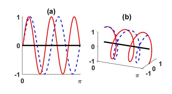
Figure 1: [color online] (a) Interlacing of eigenfunctions of the Hermitian square-well potential on the real axis. Between any two zeros of $\psi_{4}(x)=\sin\,4x$ (red solid curve) lies exactly one zero of $\psi_{3}(x)=\sin\,3x$ (blue dashed curve). (b) Winding of eigenfunctions of the square-well potential in the complex plane. Note that $\psi_{4}(x)=e^{4ix}$ (red solid curve) and $\psi_{3}(x)=e^{3ix}$ (blue dashed curve) both wind about the $x$-axis; $\psi_{4}(x)$ and $\psi_{3}(x)$ also wind about one another (see Sec. V).

An explanation of these winding numbers employs two standard theorems on Hermitian Sturm-Liouville problems; namely, differential equations of the general form

$$-Eh(x)\psi(x)=\frac{d}{dx}\left[f(x)\frac{d\psi(x)}{dx}\right]+g(x)\psi(x).$$

We first note that for a rising potential $V(x)$ the Schrödinger equation

$$i\psi_{t}(x,t)=-\psi_{xx}(x,t)+V(x)\psi(x,t)$$

possesses a countably infinite number of stationary solutions $\psi_{n}(x,t)=\psi_{n}(x)e^{-iE_{n}t}$, $E_{n}\in\mathbb{R}$, governed by the time-independent Schrödinger eigenvalue equation

$$E\psi(x)=-\psi_{xx}(x)+V(x)\psi(x),$$ (1)

which is in Sturm-Liouville form. The Sturm-Picone Comparison Theorem in our case is equivalent to the statement that the eigenfunctions of a Hermitian Hamiltonian interlace. The Sturm Separation Theorem considers any two linearly independent solutions $u(x)$ and $v(x)$ corresponding to the same eigenvalue of a Sturm-Liouville problem without boundary conditions imposed. The theorem states that $u(x)$ and $v(x)$ must have the same number of nodes and that $u(x)$ and $v(x)$ exhibit a type of interlacing. Between any two consecutive nodes of $u(x)$ lies exactly one node of $v(x)$ and vice versa.

For Hermitian Hamiltonians, we may always take $u(x)$ and $v(x)$ to be real valued. The Sturm Separation Theorem implies that all extended Hermitian eigenfunctions $\psi_{n}(x)=c_{1}u_{n}(x)+ic_{2}v_{n}(x)$ with $c_{1},c_{2}\in\mathbb{R}$ exhibit winding. Furthermore, adjusting the boundary conditions to approach the limit $c_{2}\to 0$ corresponds to approaching the proper eigenfunctions $\psi_{n}(x)$ that exhibit degenerate winding number and Hermitian interlacing.

As an example, let us reconsider the square-well potential. Before we impose boundary conditions, our extended eigenfunctions are

$$\psi_{n}(x)=c_{1}\sin(nx)+ic_{2}\cos(nx).$$

By choosing $c_{1}=c_{2}=1$, we can calculate exactly the winding of

$$\psi_{n}(x)=\sin(nx)+i\cos(nx)=ie^{-inx}$$

to be $n\pi$, as the eigenfunctions are perfect helices about the x-axis. Other choices $c_{1}\neq c_{2}$ correspond to helices with elliptical (not circular) projections onto the plane [Re$\,\psi_{n}(x)$, Im$\,\psi_{n}(x)$] with the same overall winding number. The eccentricity of the ellipse grows as $c_{2}\to 0$ but the winding number remains the same. The degenerate limiting case $c_{2}=0$ corresponding to the correct boundary conditions projects onto a line, which reduces to the flat, Hermitian case of $\psi_{n}(x)=c_{1}\sin(nx)$.

The prior two explanations are fundamentally the same because the analytic extension $\sin(nx)\to\sin(nz)$ may be expressed as $\sin(nx+iny)=\sin(nx)\cosh(ny)+i\cos(nx)\sinh(ny)$. Curves along which ${\rm Im}\,z=y_{0}$ remains constant correspond precisely to linear combinations of the linearly independent solutions $\sin(nx)$ and $\cos(nx)$, albeit with imposed boundary condition $\psi_{n}(iy_{0})=\psi_{n}(\pi+iy_{0})=i\,\sinh y_{0}$. In general, analytic extensions of the eigenfunctions of Hermitian Sturm-Liouville problems always correspond to complex sums of their two linearly independent solutions.

I.2 Harmonic oscillator potential

Sturm-Liouville problems with boundary conditions at infinity also exhibit distinct and well-ordered windings. For example, consider the harmonic-oscillator potential $V(x)=x^{2}$ with eigenfunctions that vanish at $\pm\infty$. The solutions to this problem are

$$\psi_{n}(x)=H_{n}(x)e^{-x^{2}/2},$$

where $H_{n}(x)$ is the $n$th Hermite polynomial. We again perform a complex extension and find the winding numbers of the extended eigenfunctions

$$\psi_{n}(x+i\epsilon)=H_{n}(x+i\epsilon)e^{(x+i\epsilon)^{2}/2}.$$

For $\epsilon\neq 0$, the system corresponds to the unbroken $\mathcal{PT}$-symmetric shifted harmonic oscillator problem $V(x)=(x+i\epsilon)^{2}$ R8 . The term $e^{(x^{2}-\epsilon^{2})/2}$ does not contribute to the winding of the eigenfunctions. The $e^{i\epsilon x}$ term adds to each eigenfunction an infinite number of winds about the $x$-axis independent of $n$. The distinctness of the eigenfunction windings arises from the remaining term; that is, the Hermite polynomials:

$$H_{0}(x+i\epsilon) = 1,$$

$$H_{1}(x+i\epsilon) = 2x+2i\epsilon,$$

$$H_{2}(x+i\epsilon) = 4x^{2}-4\epsilon^{2}-2+4i\epsilon x,$$

$$H_{3}(x+i\epsilon) = x^{3}-3\epsilon^{2}x-12x-i(12\epsilon-3\epsilon x^{2}+3\epsilon^{3}).$$

By integrating, we find that $H_{n}(x+i\epsilon)$ winds $n\pi$ times about the $x$-axis. Therefore, the infinities cancel; that is, $W[\psi_{n}(x)]-W[\psi_{m}(x)]=(m-n)\pi$. The eigenfunctions are well-ordered even though the windings are infinite. We plot the projections $({\rm Re}H_{n},{\rm Im}H_{n})$ of the first few Hermite polynomials in Fig. 2. Also, we note that in the Hermitian limit $\epsilon\to 0$, the infinite winding term $e^{i\epsilon x}$ completely disappears from the eigenfunctions. Once more we observe the degenerate and finite signature of winding; namely, interlacing on the real axis.

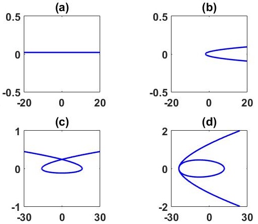
Figure 2: (a)-(d) Projections of the complex Hermite polynomials $H_{n}(x+i\epsilon)$ onto the plane $(\text{Re}\,H_{n},\,\text{Im}\,H_{n})$ for fixed $\epsilon=0.001$ and $n=1,\,2,\,3,\,4$. Each additional half-loop traversed by a curve corresponds to an additional winding of $\pi$ traversed by the eigenfunctions of the $\mathcal{PT}$-symmetric harmonic oscillator.

I.3 $\mathcal{PT}$-symmetric cubic potential

Next, we consider the $\mathcal{PT}$-symmetric potential $V(x)=ix^{3}$ on a finite domain with eigenfunctions that are required to vanish at $x=\pm L$ R3 . This equation is not analytically soluble, so we perform a WKB analysis of the time-independent Schrödinger equation

$$-\epsilon^{2}\psi^{\prime\prime}(x)=[E-V(x)]\psi(x)$$

in order to determine the behavior of high-energy eigenfunctions. We treat the parameter $\epsilon$ as small although we will eventually set $\epsilon=1$. The WKB approximation for $n>>1$ is

$$\psi_{n}(x)\sim\frac{C_{\pm}}{[E_{n}-V(x)]^{1/4}}\exp\left[\pm\frac{i}{\epsilon}\int^{x}\!\!ds\sqrt{E_{n}-V(s)}\right].$$

Setting $\psi(-L)=0$ implies that

$$\psi_{n}(x)\sim\frac{C}{[E_{n}-V(x)]^{1/4}}\sin\left[\frac{1}{\epsilon}\int^{x}_{-L}\!\!ds\sqrt{E_{n}-V(s)}\right].$$ (2)

We further impose $\psi(L)=0$ and find that

$$n\pi\sim\frac{1}{\epsilon}\int_{-L}^{L}ds\sqrt{E_{n}-V(s)}.$$

Hence, for large $E_{n}$, we get

$$E_{n}\sim\frac{n^{2}\pi^{2}\epsilon^{2}}{4L^{2}}.$$ (3)

Substituting (3) into (2) and setting $\epsilon=1$, we get

$$\psi_{n}(x)\sim C\left[\frac{n^{2}\pi^{2}}{4L^{2}}-V(x)\right]^{-1/4}\sin\!\int^{x}_{-L}\!ds\sqrt{\frac{n^{2}\pi^{2}}{4L^{2}}-V(s)}.$$

The term $C\left[n^{2}\pi^{2}/(4L^{2})-V(x)\right]^{-1/4}$ contributes the same amount of winding for each eigenfunction. Thus, we need only consider the effect of the sine term. Substituting $V(s)=is^{3}$ and making a binomial approximation to the square root, we find that

$$\sin\!{\int_{-L}^{x}\!ds\sqrt{\frac{n^{2}\pi^{2}}{4L^{2}}-is^{3}}}\!\! \sim \!\!\sin\!\left(\frac{n\pi x}{2L}\right)\cosh\left[\frac{n\pi(L^{4}-x^{4})}{16L}\right]$$

$$-\cos\left(\frac{n\pi x}{2L}\right)\sinh\left[\frac{n\pi(L^{4}-x^{4})}{16L}\right].$$

Since $\sinh y\sim\cosh y$ for large positive $y$, we get

$$\sin{\int^{x}_{-L}ds\,\sqrt{\frac{n^{2}\pi^{2}}{4L^{2}}-is^{3}}}\sim D_{n}\exp\left[\frac{-in\pi x}{2L}\right],$$

which has winding number $n\pi$ on $-L\leq x\leq L$.

For many non-Hermitian potentials, as long as $L$ remains finite, the high-energy eigenfunctions possess finite and distinct winding numbers. If $L$ is infinite, the eigenfunctions may possess infinite but still well-ordered winding numbers. To understand this behavior we consider the complex extensions of the eigenfunctions $\psi_{n}(x)\to\psi_{n}(z)$. There exists a complex contour $\mathcal{C}_{1}$ between the turning points of $\psi_{n}(z)$ on which $\psi_{n}(z)$ is entirely real. Furthermore, $\psi_{n}(z)$ has exactly $n$ nodes on this path. However, on the other sides of the turning points there exist constant-phase contours $\mathcal{C}_{2}$ and $\mathcal{C}_{3}$ from the location of the turning point out to infinity on which the eigenfunction possesses a constant angular argument and never vanishes R7 ; R9 . Thus, eigenfunctions defined along the curve $\mathcal{C}=\mathcal{C}_{1}+\mathcal{C}_{2}+\mathcal{C}_{3}$ possess a Hermitian-like degenerate winding $n\pi$. Continuously deforming $\mathcal{C}$ to the real axis pulls the eigenfunction out of the well-behaved-phase region into an oscillatory region and induces infinite but distinct windings, like the $\mathcal{PT}$-symmetric shifted harmonic oscillator discussed in Subsec. IB.

I.4 Exceptional points

To describe fully the class of $\mathcal{PT}$-symmetric Hamiltonians, we insert a parameter $\epsilon$ into a $\mathcal{PT}$-symmetric potential $V(x)\to V(x;\epsilon)$. By varying $\epsilon$, we may vary the degree of symmetry or symmetry-breaking present in the system. By convention, we insert $\epsilon$ in such a way that $V(x;0)$ is Hermitian. A value of $\epsilon$ at which the Hamiltonian operator is singular, that is, at which at least one pair of eigenfunctions possesses the same eigenvalue, is called an exceptional point. Past an exceptional point (in a region of broken $\mathcal{PT}$ symmetry) one or more pairs of eigenvalues are complex conjugates and their corresponding eigenfunctions satisfy $\psi_{1}(x)=c\,\psi_{2}^{*}(-x)$, where $c$ is some complex constant. We define the degree of symmetry breaking of a Hamiltonian $H(x,\epsilon_{0})$ as the number of its eigenvalues that are paired or complex-valued.

We find that distinctness and well-ordering of winding hold for both Hermitian and unbroken $\mathcal{PT}$-symmetric systems. These properties break down in a specific manner at exceptional points. In the region of broken $\mathcal{PT}$ symmetry, well-ordering of windings still holds for the eigenfunctions with corresponding real eigenvalue. However, extended interlacing need not hold for eigenfunctions with complex eigenvalue. That is, a higher degree of symmetry breaking corresponds to well-ordering by winding of fewer eigenfunctions. These properties need not hold for general non-Hermitian systems lacking $\mathcal{PT}$ symmetry (see Fig. 3).

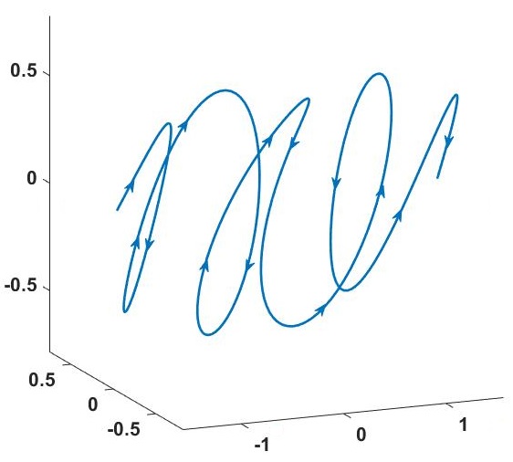
Figure 3: Ninth eigenfunction of the non-Hermitian potential $V(x)=x\,\sin x+i\epsilon\cos(3x)$ for $\epsilon=20$ plotted as the curve $[x,\,{\rm Re}\,\psi(x),\,{\rm Im}\,\psi(x)]$ on the interval $-\pi/2\leq x<\pi/2$. Observe that eigenfunctions of an arbitrary non-Hermitian system need not behave as well as eigenfunctions of a Hermitian or $\mathcal{PT}$-symmetric system. As we increase $\epsilon$ in $V(x)$ from 0 to 20, the system passes through singularities, and thus eigenfunction windings change in an irregular manner compared to that of a $\mathcal{PT}$-symmetric system. The plotted eigenfunction has winding number zero because the phase loops twice about the $x$-axis in one direction, turns around, and then makes two loops in the opposite direction. Thus, in terms of phase angle, $W[\psi_{9}(x)]=\int_{\pi/2}^{\pi/2}\theta_{x}(x)dx=0$.

Having explained how the phase angles $\theta_{n}(x)$ of unbroken $\mathcal{PT}$-symmetric eigenfunctions $\psi_{n}(x)$ depend locally on $x$, for the remainder of the paper, we discuss the winding of eigenfunctions in a global sense, that is, as functions of a parameter $\epsilon$. This paper is organized as follows. We describe the dependence of eigenfunction winding on the degree of symmetry breaking present in linear and nonlinear time-independent Schrödinger equations in Sec. II. In Sec. III we demonstrate winding in a previously studied nonlinear differential equation problem exhibiting ordered oscillations. Section IV examines the property of well-ordered winding in higher-dimensional systems. Finally, in Sec. V, we summarize these results and offer concluding remarks.

II Parametric Dependence of Winding on $\epsilon$

A theorem of Sturm states that the zeros of the real-valued eigenfunctions of Hermitian Hamiltonians interlace. In Sec. I, we demonstrated that this interlacing is a degenerate, limiting signature of the more general phenomenon of eigenfunction winding in the complex plane. We may observe this winding by integrating the differential equation from one boundary point to the other along a path through the complex plane instead of along the real axis. We may also see this winding by perturbing the boundary conditions on the eigenfunction into the complex plane and then taking the limit as the boundary conditions approach the real axis. Unbroken $\mathcal{PT}$-symmetric Hamiltonians exhibit the same winding behavior as Hermitian systems.

We can study the universal nature of winding in Hermitian and $\mathcal{PT}$-symmetric systems by examining parametrized classes of Hamiltonians such as the $\mathcal{PT}$-symmetric harmonic oscillator $V(x)=(x+i\epsilon)^{2}$ in Sec. IB. This example lacks phase transitions: the winding number of each eigenfunction is uniform for all values $\epsilon\neq 0$. We now turn our focus to systems with exceptional points.

When we vary $\epsilon$ in a region of unbroken $\mathcal{PT}$ symmetry, the eigenfunctions of $\mathcal{H}(x,\epsilon)$ deform continuously, with two exceptions: the flattening of infinite winding on an infinite domain at the point of Hermiticity (like the harmonic oscillator) or the formation of a singularity in the operator perhaps due to the breaking of a symmetry other than $\mathcal{PT}$ symmetry. We now explain the general phenomenon of well-ordered windings R7 as a consequence of the absence of eigenfunction nodes on the real axis in a region of unbroken symmetry.

Why do eigenfunctions lack nodes on the real axis? As long as the value of $\epsilon$ does not correspond to an exceptional point, the operator $\mathcal{H}(x,\epsilon)$ is nonsingular. Thus, for a fixed nonexceptional value of $\epsilon$, we may take a polar decomposition of any eigenfunction $\psi(x)=r(x)e^{i\theta(x)}$. If $\psi(x)$ vanishes at some point $x=x_{0}$, then $r(x_{0})=0$. Furthermore, $r(x)$ is always nonnegative, so $r_{x}(x_{0})=0$. Thus, $\psi_{x}(x_{0})=[r(x_{0})+ir_{x}(x_{0})\theta(x_{0})]e^{i\theta(x_{0})}=0$. The vanishing of $\psi(x)$ and $\psi_{x}(x)$ at $x=x_{0}$ implies that all derivatives of $\psi(x)$ vanish at $x=x_{0}$ because $\psi(x)$ obeys the Schrödinger equation. If all derivatives of an analytic function are zero at a point, then that function is constant. But $\psi(x)=0$ contradicts the assumption that $\psi(x)$ is an eigenfunction. Thus, $\psi(x)$ does not vanish on the real axis.

Because eigenfunctions of unbroken $\mathcal{PT}$-symmetric operators are nodeless, their windings may not exhibit any sudden discontinuities as we vary $\epsilon$. Thus, the windings of eigenfunctions vary continuously in the region of unbroken $\mathcal{PT}$ symmetry. This in turn leads to the winding-number-based ordering of eigenfunctions in these potentials.

What happens at an exceptional point (where the operator is singular)? As $\epsilon$ approaches an exceptional point, a pair of solutions begins to coalesce. At the exceptional point, these two eigenfunctions are identical and therefore possess the same winding number. Past the exceptional point, the solutions $\psi_{1}$ and $\psi_{2}$ are $\mathcal{PT}$ conjugates, so they still have the same winding number: $W[\psi_{1}(x)]=W[\psi_{2}(x)]$.

The $\epsilon$ dependence of eigenfunctions with complex eigenvalue is distinct from that of eigenfunctions with real eigenvalue. As we parametrically pass through an exceptional point, the windings of the eigenfunctions undisturbed by the crossing with real corresponding eigenvalue remain ordered with respect to one another in the same manner as prior to the crossing. However, eigenfunctions having complex eigenvalues need not respect that order.

The eigenfunctions of a non-Hermitian Hamiltonian $\mathcal{H}(x;\epsilon)$ that lacks symmetry do not necessarily exhibit any of these characteristics. Due to the lack of consistency in singularity formation in $\mathcal{H}(x;\epsilon)$ with respect to the parameter $\epsilon$, eigenvalues may develop multiplicities or become complex in a nonuniform fashion. Eigenfunctions may also develop nodes unsystematically and do not shift windings in a prescribed manner past a singular point. Thus, deformations of non-Hermitian Hamiltonians do not have to maintain strict eigenvalue-based order or well-predicted pairings of winding numbers.

The statements above appear to hold for all potentials, whether or not they are periodic. However, the extra constraints that periodicity places on a system lead to noticeable differences in the winding variations in $\epsilon$. We present two examples to highlight these differences. We then examine how similar properties appear even when the system is nonlinear.

II.1 Nonperiodic potential

Consider first the linear Schrödinger eigenvalue equation (1) with the nonperiodic $\mathcal{PT}$-symmetric potential

$$V(x)=4-4i\epsilon x$$

on the finite interval $[-\pi/2,\pi/2]$. We impose homogeneous boundary conditions at the endpoints. As predicted, the eigenfunction windings deform smoothly and continuously in the region between two exceptional points. At an exceptional point, the winding numbers of two eigenfunctions merge. The exceptional point is the sole point of nonsmooth variation of winding numbers; the derivative $\frac{dW_{n}}{dt}$ may be different on either side of the transition. Beyond an exceptional point, however, these winding numbers vary smoothly once more and in tandem. That is, nonsmooth winding deformation occurs only at an exceptional point and only for the specific eigenfunctions with coalesced eigenvalues. We plot the phase of the eigenfunctions at each $(x,\epsilon)$ value in Fig. 4.

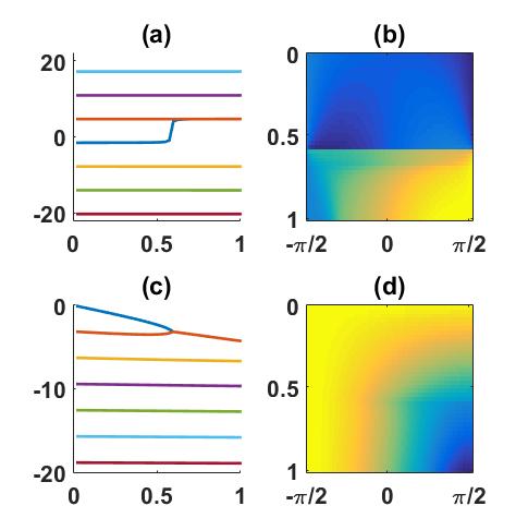
Figure 4: [color online] Dependence of eigenfunction winding on the parameter $\epsilon$ for the nonperiodic potential $V(x)=4-4i\epsilon x$ (panel a) and the periodic potential $V(x)=4\cos^{2}x+4i\sin(2x)$ (panel c). The corresponding phase angles $\theta(x,\epsilon)$ of the first eigenfunction of each potential for a range of $(x,\epsilon)$ are shown in (b) and (d). Note the sharp jump discontinuity in both eigenvalue magnitude and eigenfunction phase-angles function at an exceptional point [panel (b)], compared to the continuous dependence on $\epsilon$ for the nonperiodic potential [panel (d)].

II.2 Periodic potential

The eigenfunctions of a $\mathcal{PT}$-symmetric periodic potential, unlike those of a nonperiodic potential, always possess winding numbers that are equivalent modulo $2\pi$. This property is due to Bloch’s theorem, which states that solutions to a Schrödinger equation with a periodic potential take the form

$$\psi_{n}(x)=u_{n}(x)e^{ikx},$$

where $-\pi\leq k<\pi$ is a chosen Bloch wavenumber. Thus, any change in winding must occur as a discontinuous jump. As we approach an exceptional point the behavior of the eigenfunctions is not immediately apparent.

Thus, let us examine the complex phase at every point of the wave. We consider the potential

$$V(x)=4\cos^{2}x+4i\epsilon\sin(2x),$$ (4)

which was studied in Ref. R10 . We first find the eigenfunctions for $k\neq 0$. Figure 4 shows that in the region of unbroken symmetry the eigenfunctions have winding numbers $W_{2n}=-W_{2n+1}$. The approach towards an exceptional point is marked not only by the formation of a sharp cusp in eigenfunction magnitude but also by the corresponding formation of a jump discontinuity in eigenfunction phase. The eigenfunction tries to complete a full loop about the $x$-axis within an extremely short distance. As that length reaches zero, the system crosses an exceptional point and the eigenfunction winding jumps. Interestingly, only one eigenfunction of the pair exhibits this type of dependence on $\epsilon$ rather than a mutual merging as observed in the nonperiodic case. At $\epsilon=0.5$, all the bands go complex simultaneously at their edges $k=\pm 1$. At this parameter value, the eigenfunctions have exact solutions in terms of Bessel functions R10 :

$$u(x)=J_{k}(i\sqrt{\epsilon/2}\,e^{ix}).$$

Here, we calculate that $u(x)$ has winding number $\pi$.

We remark that some Hamiltonian systems may have more complicated variations in eigenfunction pairings; one example is $V(x)=\cos^{2}x+i\epsilon\sin^{3}(2x)$. The restrictions placed on winding number by complex conjugacy pairings, coupled with the absence of nodes, helps to explain their more nuanced behaviors.

II.3 Cubic nonlinearity

Many $\mathcal{PT}$-symmetric nonlinear Schrödinger equations exhibit similar characteristics to their linear counterparts. Let us first examine a Schrödinger equation with an additive Kerr, or cubic ($|\psi|^{2}\psi$), nonlinearity

$$E\psi(x)=-\psi_{xx}(x)+V(x)\psi(x)+|\psi(x)|^{2}\psi,$$

This equation is isomorphic to the nonlinear paraxial wave equation governing the propagation of intense light through a waveguide. For Fig. 5, we analyze the extended stationary states of a periodic potential (4) R11 ; R12 . To find these states we choose a wave intensity

$$P_{uc}=\int dx|\psi(x)|^{2}$$

over the unit cell. The value of $P_{uc}$ determines the reality or complexity of the band structure R12 . Thus, adjustment of the parameters $P_{uc}$ and $E$ allows us to change the degree of symmetry breaking present at each part of the spectrum. Singular points correspond to jumps in winding in a manner similar to the linear case. This type of eigenfunction winding evolution occurs regardless of the variable ($P_{uc}$, $k$, or $\epsilon$) by which we approach an exceptional point.

If we perform the same procedure with the nonintegrable Schrödinger system with quintic nonlinearity

$$E\psi(x)=-\psi_{xx}(x)+V(x)\psi(x)+|\psi(x)|^{4}\psi(x),$$

using the potential in (4), we again find that eigenfunction windings appear to be well ordered as in the linear and cubic-nonlinear cases.

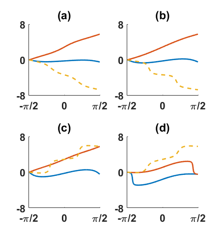
Figure 5: [color online] Phase angle at every point of the first three eigenfunctions (solid blue, solid red, dashed yellow) of the Schrödinger equation with additive cubic ($|\psi|^{2}\psi|$) nonlinearity and potential $V(x)=4\cos^{2}x+4i\epsilon\sin(2x)$ for $\epsilon=0.25,\,0.50,\,0.75,1.00$ in panels (a)-(d). All of the eigenfunctions have real corresponding eigenvalue except for the first and second eigenfunctions, which have become $\mathcal{PT}$ conjugates [panel (d)]. Note the approach towards a jump discontinuity in phase angle near a singular point. The third eigenfunction is always associated with a real eigenvalue, and the jump in its winding for $\epsilon\in(0.50,0.75)$ does not occur because of $\mathcal{PT}$ symmetry breaking.

III Winding Interpretation of Initial-Value Problem

In this section we consider the nonlinear first-order initial-value problem

$$y^{\prime}(x)=\cos[\pi xy(x)],\hskip 14.22636pty(0)=a.$$ (5)

The solutions to this non-Sturm-Liouville problem for real $a$ on the interval $[0,\infty)$ were described in R13 . The solutions exhibit oscillations that look strikingly similar to the interlacing properties of Sturm-Liouville systems. All solution curves with initial conditions in a range $a_{n}<a<a_{n+1}$ exhibit the same number of up-and-down oscillations. The values $...,a_{-1},a_{0},a_{1},...a_{n},...$ correspond to separatrix solutions with oscillation number intermediate between the solutions with initial condition on either side.

III.1 Winding dependence on initial $y$ condition

If we perturb the initial condition $a$ into the complex plane, $y(x)$ winds in the space $[x,\text{Re}\,y(x),\text{Im}y(x)]$, though not about the axis $x=0$. The winding number of $y(x)$ on the interval $[0,\infty)$ is dependent on the initial condition $a$. Initial conditions within specific two-dimensional regions of complex initial condition space all induce the same winding number. These regions appear to be separated by curves of initial conditions inducing separatrix-like behavior (see Fig. 6).

Figure 6: [color online] Selected complex initial conditions and the winding numbers to which they give rise for (5). A red dot indicates a winding of $\pi$, a blue $x$ indicates a winding of $3\pi$, and a green $+$ indicates a winding $5\pi$. It appears that adjacent regions are separated by a curve of initial conditions, which give rise to separatrix solutions.

III.2 Winding dependence on initial $x$ condition

Let us take (5) with initial condition $y(b)=a$, with $b$ not necessarily zero. We simplify notation by shifting the equation to get

$$y^{\prime}(x)=\cos[\pi(x-b)(y-a)],\quad y(0)=0.$$ (6)

When we impose $y^{\prime}(0)=1$, a condition that always holds for (5), we find that $b$ may take on only a countably infinite number of values $b_{n}=2n/a$. We denote the solution corresponding to parameter $b_{n}$ as $y_{n}(x)$.

We now examine a set of $y_{n}(x)$ for positive $n$. If $a$ is suitably small, we find that solution curves have well-ordered winding numbers on the interval $[0,\infty)$. As we increase $a$, the winding numbers of one or multiple $y_{n}(x)$ exhibit sudden shifts (see Fig. 7). The initial condition $b_{n}$ acts in a topologically-similar manner to an eigenvalue in a Schrödinger equation, and $a$ behaves similarly to the exceptional-point parameter $\epsilon$. Because (5) lacks nodal interlacing, these parallels only become apparent when we perturb these initial conditions into the complex plane and observe winding.

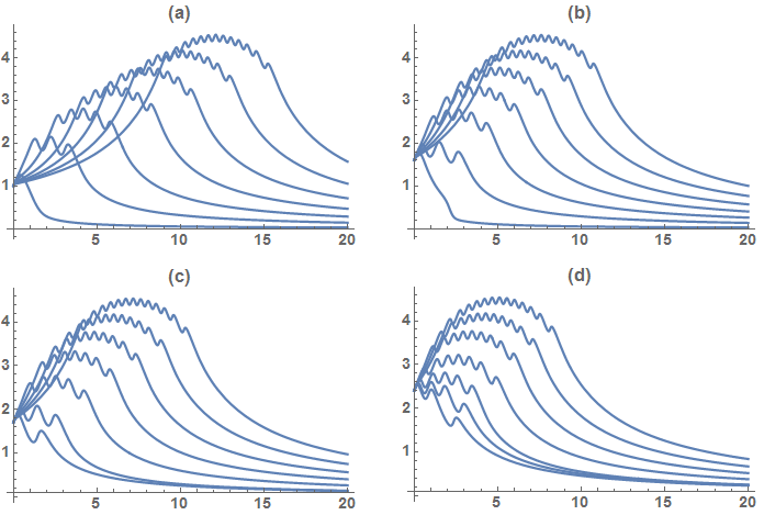
Figure 7: First seven eigenfunctions of the extended cosine problem $y^{\prime}(x)=\cos[-2\pi n\psi(x)/\epsilon]$ with initial conditions $y^{\prime}(0)=\epsilon$ and $y^{\prime}(0)=1$ for $\epsilon=1.0,\,1.6,\,1.7,\,2.4$ in panels (a)-(d). On the interval $[0,\infty)$, these eigenfunctions have $(4n+1)$ extrema, the degenerate signature of winding number $(2n+1)\pi$. At each exceptional point, one or multiple eigenfunctions each gain two local extrema, or $\pi$, of winding.

Therefore, (5) behaves like a precise first-order differential equation model with an exceptional-point parameter or, alternatively, like the lowest eigenfunction of a much broader set of differential equations. In this context the asymptotic calculations presented in Ref. R13 mimic the calculation of exceptional point, or operator singularity, locations. Thus, the construction of a differential equation or its parametrization may affect the topology of solutions. The careful addition of extra parameters or perturbation into the complex plane may enhance our understanding of the nature of solutions and the origin of winding phenomena.

Now, let us return to (6) and consider negative-$n$ states. On $[0,\infty)$ for $a=0$, each solution has only one local extremum. That is, for complex $a$, $W[y_{-n}(x)]=\pi$ for all $n$. However, as we increase $a$, the negative-$n$ solutions develop extra oscillations (winds) two at a time, just as the positive-$n$ solutions do. When we broaden our outlook to the full real domain, we notice a pairing phenomenon similar to that of $\mathcal{PT}$-symmetric systems (see Fig. 8). While $y_{n}(x)$ and $y_{-n}(x)$ may differ in winding number at $a=0$, as $a$ increases, they eventually pair off: possessing the same winding number and approaching translations of one another along the $x$-axis.

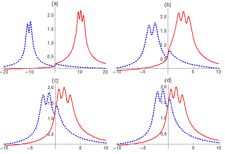
Figure 8: [color online] Solutions to $y_{\pm}^{\prime}(x)=\cos[\pi(x\pm 2\epsilon)y_{\pm}(x)]$ for $\epsilon=0.5,\,0.7,\,1.3,\,1.5$ for panels (a)-(d). As $\epsilon$ increases, $y_{+}(x)$ (red solid curve) and $y_{-}(x)$ (blue dashed curve) pair up and approach translations of one another along the $x$-axis, similar to the pairing of eigenfunctions in $\mathcal{PT}$-symmetric Schrödinger systems.

These properties beg whether there exist other general mathematical features to distinguish negative-$n$ solutions from one another prior to the crossing of singular points in the parameter $a$.

IV Multidimensional Systems

Winding is not unique to the eigenfunctions of one-dimensional systems. The solutions to a complex N-dimensional Schrödinger equation

$$E\psi(\vec{x})=-\nabla^{2}\psi(\vec{x})+V(\vec{x})\psi(\vec{x})$$

are N-dimensional manifolds looping about the $x_{1}$-plane in an $(N+2)$-dimensional space. As in Sec. II we may show that $\mathcal{PT}$-symmetric potentials $H(\vec{x};\epsilon)$ may not possess nodes except at an exceptional point. Thus, we may begin to visualize an $N$-dimensional extension of winding based on how many times the manifold wraps around its domain, that is, the topological degree of the mapping. To see this, we consider two examples.

IV.1 Square-well potential

We start with the $n$-dimensional square-well potential $V(\vec{x})=0$. This equation has separated solutions $\psi_{a_{1}a_{2}...a_{n}}(\vec{x})=\psi_{a_{1}}(x_{1})...\psi_{a_{n}}(x_{n})$, where $n$ integer parameters $a_{k}$ are necessary to describe the eigenfunction. The $\psi_{a_{i}}(x_{i})$ terms are each solutions to the one-dimensional version of this system seen in Sec. I, $\psi_{a}(x)=\sin(ax)$. If we move the boundary conditions into the complex plane, the eigenfunctions begin to exhibit monotonically increasing phase angles in each positive $x_{i}$ direction. Just as in Sec. I, we can perturb the equation so that the eigenfunctions are of the form

$$\psi_{a_{1}...a_{n}}(\vec{x})=e^{ia_{1}x_{1}}e^{ia_{2}x_{2}}...e^{ia_{n}x_{n}}.$$

This perturbation does not appear to affect the phase angle at any point $\vec{x}$, and thus the overall $n$-dimensional winding number is the same as in the limit of vanishing boundary conditions. This function increases in phase angle by $(a_{1}+...+a_{n})\pi$ from the top left corner to the bottom right corner of the domain.

IV.2 Harmonic oscillator

Like the square-well potential, the $n$-dimensional harmonic oscillator has separated eigenfunction solutions

$$\psi_{a_{1}...a_{n}}=e^{x_{1}^{2}+...+x_{n}^{2}}H_{a_{1}}(x_{1})...H_{a_{n}}(x_{n})$$

defined by $n$ parameters $a_{i}$. When we perturb $x_{i}\to x_{i}+i\epsilon_{i}$, the eigenfunctions exhibit infinite winding due to the term exp[$\sum_{n}i\epsilon_{n}x_{n}$]. However, this term contributes the same infinite amount of winding for any choice $a_{1},...,a_{n}$. The Hermite polynomials add distinctness and order of eigenfunction windings in the system (see Fig. 9). Multidimensional systems with exceptional points will be explored in future work.

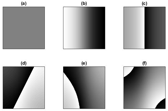
Figure 9: Two-dimensional plot of the phase angle $\theta(\vec{x})$ modulo $2\pi$ of $\psi(\vec{x})=r(\vec{x})e^{i\theta(\vec{x})}$ for the two-dimensional harmonic oscillator with both $\vec{x}$ components on the interval $[-20,20]$, for $(m,n)=(0,0),\,(1,0),\,(2,0),\,(1,1),\,(2,1),\,(2,2)$ in panels (a)-(f). Lighter color corresponds to increasing phase angle from $-\pi$ to $\pi$. In general, eigenfunctions of an $N$-dimensional $\mathcal{PT}$-symmetric Schrödinger equation are $N$-dimensional manifolds in an $(N+2)$-dimensional space ($N$ spatial dimensions plus two extra dimensions for the real and imaginary parts of the value $\psi(\vec{x})$ at a point $\vec{x}$).

V Conclusions and Outlook

In this paper we have generalized the Sturm-Liouville interlacing property to ordered winding in non-Hermitian systems. The nature of these winds and their magnitude relative to one another may be studied by inserting a parameter into the system and adjusting its value past singular points. In particular, the eigenfunctions of Hermitian and unbroken $\mathcal{PT}$-symmetric systems have well-ordered winding numbers that pair up as the system passes through an exceptional point.

We have seen that similar descriptions apply to some nonlinear and higher-dimensional systems. Notably, winding characterizes wave propagation in certain time-dependent systems R14 such as the stable oscillatory solutions of the nonlinear paraxial wave equation in R12 . Additionally, the solutions to initial-value problems, such as (5) and the Painlevé transcendents, exhibit real-axis oscillatory properties that translate to winding in the complex plane R15 ; R16 . It is of interest to find out how winding manifests itself in similar systems.

Whether there exist more general statements than interlacing on the solutions of $\mathcal{PT}$-symmetric and general non-Hermitian systems remains open. One interesting question to examine might lie in the mathematical theories of braids and knots R17 , which bear resemblance to the eigenfunctions of systems with identical boundary conditions at the endpoints. For example, it is readily apparent that the extended eigenfunctions $\psi_{n}(x)=e^{inx}$ of the Hermitian square-well potential discussed in Sec. I exhibit braiding not only about the $x$-axis, but also about one another. That is, the $n$th and $(n+1)$st eigenfunctions intertwine about each other exactly $n$ times [see, for example, Fig. 1(b)]. We cannot deform the eigenfunctions so that they become unwound without moving their endpoints. It follows that symmetry-breaking exceptional points demarcate a change in braiding of the eigenfunctions. If generally true, such an interlacing extension might help further unravel solution behaviors.

To gain a fundamental understanding of the nature of both Hermitian and $\mathcal{PT}$-symmetric systems, it is often necessary to broaden our perspective into the complex plane. We have extended Hermitian interlacing properties to non-Hermitian $\mathcal{PT}$-symmetric Sturm-Liouville problems. We hypothesize that similar analyses may provide insights into nonlinear and higher-dimensional systems described by broader classes of ordinary- and partial-differential equations. These have potential ramifications for understanding systems in applied disciplines.

STS thanks H. Herzig Sheinfux, Y. Lumer, and M. Segev for helpful discussions and assistance. Figures were generated using MATLAB and Mathematica.

References

- (1) A. Guo, G. J. Salamo, D. Duchesne, R. Morandotti, M. Voltier-Ravat, V. Aimez, G. A. Sivilglou, and D. N. Christodoulides, Phys. Rev. Lett. 103, 093902 (2009).
- (2) C. E. Rüter, K. G. Makris, R. El-Ganainy, D. N. Christodoulides, M. Segev, and D. Kip, Nat. Phys. 6, 192 (2010).
- (3) C. M. Bender and S. Boettcher, Phys. Rev. Lett. 80, 5243 (1998).
- (4) C. M. Bender, Rep. Prog. Phys. 70, 947 (2007).
- (5) Z. Lin, H. Ramezani, T. Eichelkraut, T. Kottos, H. Cao, and D. N. Christodoulides, Phys. Rev. Lett. 106, 213901 (2011).
- (6) A. Regensberger, C. Bersch, M.-A. Miri, G. Onishchukov, and D. N. Christodoulides, Nat. 488, 167 (2012).
- (7) N. Chtchelkatchev, A. Golubov, T. Baturina, and V. Vinokur, Phys. Rev. Lett. 109, 150405 (2012).
- (8) L. Feng, Y.-L. Xu, W. S. Fegadolli, M.-H. Lu, J. E. B. Oliveira, V. R. Almeida, Y.-F. Chen, and A. Scherer Nat. Mat. 12, 108 (2013).
- (9) R. Courant and D. Hilbert, Methods of Mathematical Physics I (Interscience, New York, 1953), Chap. 6.
- (10) S. Weigert, Phys. Rev. A 68, 062111 (2003).
- (11) C. M. Bender, S. Boettcher, and V. M. Savage, J. Math. Phys. 41, 6381 (2000).
- (12) M. Znojil and G. Lévai, Phys. Lett. A 271, 377 (2000).
- (13) C. M. Bender and S. A. Orszag, Advanced Mathematical Methods for Scientists and Engineers (McGraw-Hill, New York, 1978).
- (14) S. Nixon, L. Ge, and J. Yang, Phys. Rev. A 85, 023822 (2012).
- (15) O. Cohen, T. Schwartz, J. E. Fleischer, M. Segev, and D. N. Christodoulides, Phys. Rev. Lett. 91, 113901 (2003); H. Buljan, O. Cohen, J. W. Fleischer, T. Schwartz, Z. H. Musslimani, N. K. Efremidis, and D. N. Christodoulides, Phys. Rev. Lett. 92, 223901 (2004); M. Jablan, H. Buljan, O. Manela, G. Bartal, and M. Segev, Opt. Express 15, 4623 (2007).
- (16) Y. Lumer, Y. Plotnik, M. C. Rechtsman, and M. Segev, Phys. Rev. Lett. 111, 263901 (2013).
- (17) C. M. Bender, A. Fring, and J. Komijani, J. Phys. A. 47, 235204 (2014).
- (18) S. T. Schindler, Y. Lumer, H. Herzig Sheinfux, and M. Segev (in progress).
- (19) C. M. Bender and J. Komijani, J. Phys. A 48, 475202 (2015).
- (20) C. M. Bender and S. T. Schindler (in progress).
- (21) E. Artin, Ann. Math. 48, 101 (1947).