Associative content-addressable networks with exponentially many robust stable states

Abstract

The brain must robustly store a large number of memories, corresponding to the many events encountered over a lifetime. However, the number of memory states in existing neural network models either grows weakly with network size or recall fails catastrophically with vanishingly little noise. We construct an associative content-addressable memory with exponentially many stable states and robust error-correction. The network possesses expander graph connectivity on a restricted Boltzmann machine architecture. The expansion property allows simple neural network dynamics to perform at par with modern error-correcting codes. Appropriate networks can be constructed with sparse random connections, glomerular nodes, and associative learning using low dynamic-range weights. Thus, sparse quasi-random structures—characteristic of important error-correcting codes—may provide for high-performance computation in artificial neural networks and the brain.

Introduction

Neural long-term memory systems have high capacity, by which we mean that the number of memory states is large. Such systems are also able to recover the correct memory state from partial or noisy cues, the definition of an associative memory. If the memory state can be addressed by its content, it is furthermore called content-addressable.

Classic studies of the dynamics and capacity of associative content-addressable neural memory (ACAM) have focused on connectionist neural network models commonly called Hopfield networks ^{1; 2; 3}, which provide a powerful conceptual framework for thinking about pattern completion and associative memory in the brain. Here we continue in this tradition and examine constructions of ACAM networks in the form of Hopfield networks and their stochastic equivalents, Boltzmann machines. We show that it is possible to construct associative content-addressable memory networks with an unprecedented combination of robustness and capacity.

Hopfield networks consist of binary nodes (or “neurons”) connected by symmetric (undirected) weights (Figure 1a). At each time-step, one neuron updates its state by summing its inputs; it turns on if the sum exceeds a threshold. All neurons are updated in this way, in random sequence. The network dynamics lead it to a stable fixed point, determined by the connection strengths and initial state (Figure 1b). Equivalently, stable fixed points may be viewed as minima of a generalized energy function. Any state in the basin of attraction of an energy minimum flows to the minimum as the network dynamics push the system downhill in energy (Figure 1c). The set of stable fixed points, fully determined by the network weights, are the memory states. They are robust if their basins are sufficiently large. The Boltzmann machine ⁴ is a stochastic version of the Hopfield network: Each neuron becomes active with a probability proportional to how much its summed input exceeds threshold, and the network dynamics approach and remain in the vicinity of stable fixed points of the corresponding deterministic dynamics. Hopfield networks, Boltzmann machines, and related constructions such as autoencoders have proved to be versatile statistical models for natural stimuli and other complex inputs ^{5; 6; 7; 8; 9}.

Very generally, in any representational system there is a tradeoff between capacity and noise-robustness ^{10; 11}: a robust system must have redundancy to recover from noise, but the redundancy comes at the price of fewer representational states, Figure 1d. Memory systems exhibit the same tradeoff.

A network consisting of $N$ binary nodes has at most $2^{N}$ states; memory states are the subset of stable states. We define a high-capacity memory network as one with exponentially many stable states as a function of network size (i.e., $C\sim e^{\alpha N}$, for some constant $0<\alpha\leq 1$). A high-capacity network retains a non-vanishing information rate $\rho$ ($\rho\equiv{\log(C)}/N=\alpha$) even as the network grows in size.

A robust system is one that can tolerate a small but constant error rate ($p$) in each node, and thus a linearly growing number of total errors ($pN$) with network size. Tolerance to or robustness against such errors means that the network dynamics can still recover the original state. For robustness to growing numbers of errors with network size, each memory state must therefore be surrounded by an attracting basin that grows with network size.

In sum, high-capacity memory networks must have the same order of memory states as total possible states, both growing exponentially with network size; at the same time, the basins around each memory state must grow with network size. Can these competing requirements be simultaneously satisfied in any network?

Hopfield networks with $N$ nodes and $\sim N^{2}$ pairwise analog (infinite-precision) weights can be trained with simple learning rules to learn and exactly correct up to $N/(2\log(N))$ random binary inputs of length $N$ each ¹² or imperfectly recall $0.14N$ states (with residual errors in a small fraction of nodes) ¹³. With sparse inputs or better learning rules, it is possible to store and robustly correct $\sim N$ states ^{14; 15; 16; 17}. Independent of learning rule, the capacity of the Hopfield networks is theoretically bounded at $\sim N$ arbitrary states ^{18; 19; 20}.

If higher-order connections are permitted (for instance, a third order weight connects neurons $i,j,$ and $k$ with each other), Hopfield networks can robustly store $C\sim N^{K-1}$ memories ^{21; 22}, where $K$ is the order of the weights (thus there are up to $N^{K}$ weights). This capacity is still polynomial in network size.

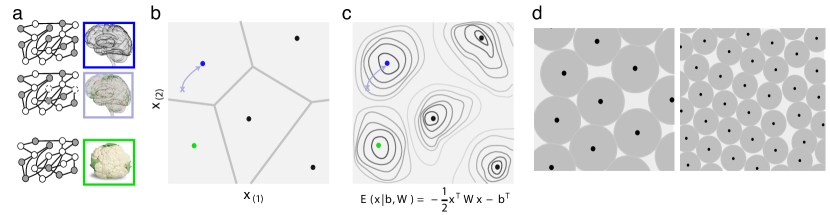
Figure 1: Hopfield networks and the robustness-capacity tradeoff. (a) Left: Schematic of different activity states in a Hopfield network (black lines: symmetric connections; dark nodes: inactive; white: active). Right: the different activity states may be viewed as corresponding to different patterns. Top and bottom depict states that are stable states of the network dynamics. Center: an intermediate state that is not a stable state. (b) Schematic state-space view of the Hopfield network. Any point in state-space corresponds to some state of the network. The dots represent stable states; the blue and green points represent the stable patterns from (a), while the lavender cross represents the intermediate state. Different stable states are separated from each other and points in the neighborhood of a stable state flow to it under the network’s dynamics (e.g., the lavender cross to the blue stable state). (c) An energy landscape view: The stable states have low energy (dots) and correspond to minima in a rugged energy landscape. Different minima are separated by energetic ridges. The network dynamics corresponds to a descent on the energy landscape to a local minimum or stable state. (d) Fundamental tradeoff between robustness and capacity: Each stable state is surrounded by a “basin of attraction” consisting of nearby states that flow to it (left). If these are viewed as noisy or corrupted copies of the stable state, the network is a decoder that performs denoising of perturbed versions of its stable (memory) states. Packing in more stable states (right) reduces the robustness of the network to noise.

Spin glasses (random-weight fully recurrent symmetric Hopfield networks) possess exponentially many local minima or (quasi)stable fixed points ^{23; 24; 21; 25}, Hopfield networks designed to solve constraint satisfaction problems exhibit $\sim 2^{\sqrt{N}}$ stable states ^{26; 27; 28}, and a recent construction with hidden nodes shows capacity that is exponential in the ratio of the number of hidden to input neurons²⁹. However, in all these cases the basins of attraction are small, with the fraction of correctable errors either shrinking with network size or negligible to begin with. Thus these networks are not robust to noise. Very recently, a capacity of $C=\sim e^{\alpha\sqrt{N}}$ was realized in Hopfield networks with particular clique structures ^{30; 31}. As required by information-theoretic constraints, the memory states do not store arbitrary input patterns. The information rate ($\rho\equiv\ln(C)/N$) of these networks still vanishes with increasing $N$ and the networks are susceptible to adversarial patterns of error: Switching a majority of nodes within one clique (but still a vanishing fraction ($\sim\sqrt{N}/N$) of total nodes in the network) results in an unrecoverable error.

The problem of robustly storing (or representing or transmitting) a large number of states in the presence of noise is also central to information theory. Shannon proved that it is possible to encode exponentially many states ($\sim e^{\alpha N},0<\alpha<1$) using codewords of length $N$ and correct a finite fraction of errors with the help of an optimal decoder ^{11; 32}. However, the complexity cost of the decoder (error-correction) is not taken into account in Shannon’s theory. Thus, it remains an open question whether an associative network, which not only represents but also implements the decoding of its memory states through its own dynamics, should be able to achieve the same coding-theoretic bound.

Here we combine the tradition of ACAM network theory with new constructions in coding theory to demonstrate a network with exponentially many stable states and basins that grow with network size so that errors in a finite fraction of all input neurons can be robustly corrected.

Note that portions of these results have been presented at conferences (R. Chaudhuri, I. Fiete Cosyne Abstracts, II-78, 2015; Soc. Neurosci. Program No. 94.05, 2015).

Results

Linear error-correcting codes embedded in ACAM networks

The codewords of linear error-correcting codes that use parity checks on binary variables can be stored as stable fixed points (equivalently, minima of the energy function) of a recurrent neural network. Consider embedding the $2^{4}$ codewords of the classic (7,4) Hamming code ³³ — well-separated by 3 bits-flips from each other (Figure 2a) — as stable fixed points in a network of 7 neurons. It is possible to do this using 4th order weights to enforce the relationships among subsets of four variables in the Hamming codewords (Figure 2b); the state of a neuron represents a corresponding bit in the codeword. By construction, codewords correspond to the energy minima of the network dynamics (Figure 2b).

Alternatively, higher order ($K$th order, where $K>2$) relationships between multiple neurons can be enforced using only pairwise weights between a set of hidden layer neurons and $K$ visible neurons in a bipartite graph (Fig. 2c).

In either case, the network dynamics do not correctly decode states: starting one bit-flip from a stable state, the network might flip a second bit, a move that is also downhill in energy but further in (Hamming) distance from the original state. The dynamics then converge to a different codeword than the original (Figure 2d) – a decoding error. Such errors are generic for Hamming codes. Starting one bit-flip from a stable state, over 50% of possible bit flips lead to a state that has lower or equal energy, and all but one of these move the network away from the correct (nearest) stable state (see SI Section 4). The error can be attributed to a failure in credit assignment: the network is unable to identify the actual flipped bit. The network’s failure should not be too surprising since in general decoding strong error-correcting codes is computationally hard ³⁴ and requires sophisticated but biologically implausible algorithms like belief propagation that do not map naturally onto simple neural network dynamics.

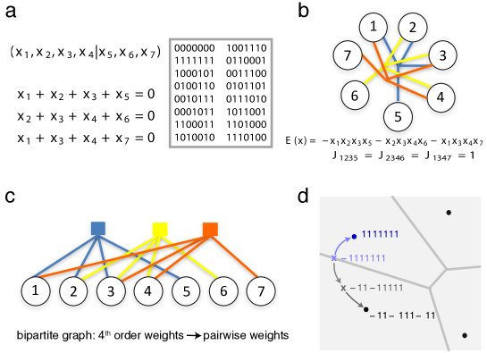
Figure 2: Linking Hopfield networks to good error-correcting codes. (a) Top left: The (7,4) Hamming code consists of 4 information-carrying bits and 3 additional bits for redundancy so that errors can be corrected. The 7-bit message must satisfy 3 constraint equations (bottom left); any solution to these equations is a permitted state or codeword (right). This code is capable of correcting all 1-bit errors (using a decoder that maps corrupted or noisy states to the nearest codeword) at a finite information rate of 4/7. (b) The Hamming codewords can be embedded as the stable states of a Hopfield network with 7 nodes, if the network is allowed to have 4th-order edges (to simplify the form of the energy function, states are mapped from $(0,1)$ to $(1,-1)$ for this Hamming implementation only). The edges simply enforce relationships between nodes (e.g. enforcing that $x_{1},x_{2},x_{3},x_{5}$ share the same activation level), to implement the (4-point) constraint equations of (a). (c) The higher-order weights can be replaced by pairwise weights if the recurrent network is transformed into a bipartite graph with a hidden layer. Here each constraint node in the hidden layer (i.e., filled squares) is not a single neuron but a network that implements a parity operation on its inputs. A sample implementation of this is shown in Fig. 4. (d) Although the neural network has energy minima at every codeword, it can fail to correctly decode even 1-bit errors. The network dynamics follows any path that reduces energy, but that path can lead to a minimum that is farther away: In the example shown, a state ($-1111111$; lavender cross) one flip away from the closest codeword ($1111111$) can proceed along two trajectories that decrease energy, one to the nearest codeword (upwards) and the other to a codeword two flips away (downwards). Note that this problem is generic: starting from a non-codeword state in the energy landscape defined by a Hamming code of length N, N/2 directions lead to lower energy states but only 1 leads to the nearest codeword.

An exponential-capacity robust ACAM

We prove that it is possible to construct an ACAM network with stable states that grow exponentially in number with the size of the network, and that can be robustly corrected by the network’s simple dynamics. Theoretical results establishing the number and robustness of these states are given in SI. Numerical simulation results on the number of stable states are shown in Figure 3a. Moreover, numerical simulations verify that the network dynamics corrects errors in a finite fraction of all the neurons in the network, meaning that the total number of correctable errors grows in proportion to network size, Figure 3b, up to a maximum corruption rate. Equivalently, given any error probability smaller than this rate, the network can correct all errors (with probability $\rightarrow 1$ as the network size goes to infinity). Typical of strong error-correcting codes, the probability of correct inference is step-like: errors smaller than a threshold size are entirely corrected, while those exceeding the threshold result in failure. Analogous results, up to small fluctuations, hold for stochastic dynamics in a Boltzmann Machine, SI Figure 2.

The specific architecture of the network makes such performance possible. The network has a two-layer structure, consisting of one layer of $N$ input neurons and one layer of constraint neurons. The constraint neurons are organized into $N_{C}\sim N$ small sub-networks, which we call constraint nodes. Each constraint neuron in a constraint node makes connections with the same set of input neurons. Thus we first describe the connectivity between input neurons and constraint nodes, Figure 4a (top). The $i$th input neuron connects to $z^{(i)}$ constraint nodes, and the $j$th constraint node connects to $z_{C}^{(j)}$ inputs, and there are no within-layer connections between input neurons or across constraint nodes. The out-degrees $z,z_{C}$ can differ across input neurons and constraint nodes, and are drawn from narrow distributions with a fixed mean that does not scale with $N$; thus the network is truly sparse. The connectivity between layers is based on sparse expander graphs ^{35; 36}, mathematical objects with widespread applications in computer science.

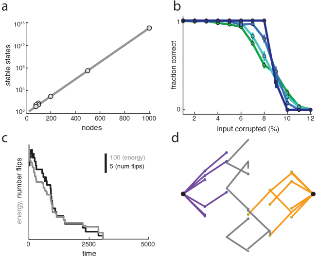
Figure 3: ACAM with exponential capacity and robust error correction. (a) Network capacity scales exponentially with number of nodes. Gray line shows theoretical results for the number of stable states (Equation 2 with $r=1$ gives the number of stable states for a network with non-overlapping parity constraints; it provides a lower bound on the networks simulated here), while open black circles show the number of stable states in sample networks. Note that the scatter of points off the line for small N reflects occasional duplicate constraints in randomly-generated networks. For larger N these duplicates are vanishingly rare, and all points lie on the line. (b) Fraction of times the network infers the correct state when a finite fraction of nodes (and thus a linearly growing number of total nodes with network size) are corrupted. Green, cyan, light blue, dark blue curves: $N=250,500,1000,1500$ respectively. We choose the input node degrees to be between 5 and 10, and the constraint node degrees to be between 2 and 6 (see SI, S6 for more details on the parameters). (c) Energy (gray) as a function of time in a simulated network of $N=500$ neurons with 4% of all nodes initially corrupted, as the network relaxes to the closest stable state. Black: the number of node flips as the network state evolves. Note that energy always decreases monotonically, but the number of node flips need not. (d) Network state-space trajectories (projected onto 2D space) in a $N=18$ neuron network, starting from 6 different initial states (with 1-5 nodes corrupted) in the vicinity of one stable state (black dot, left), with an adjacent stable state (black dot, right). Initial states closest in Hamming distance to the original stable state flow to it (lines in varying shades of blue). Those that are not flow to other stable states (remaining lines).

Once the out-degree distribution of input and constraint nodes is chosen, the connections between specific input neurons and constraint nodes is random. This procedure generically generates a sparse network with good expansion properties ^{37; 38}. As described below, the expansion property is critical for allowing the network to robustly and correctly decode noisy states.

Each constraint node is a subnetwork of neurons, all connected to the same subset of $z_{C}$ input neurons, Figure 4b. A constraint node can thus be viewed as a glomerulus. Thus, while the input-to-constraint node connectivity is random, at the level of individual constraint neurons connectivity within a node is correlated since all neurons must receive the same set of inputs – the network is not fully random. Let each neuron in a constraint node be strongly activated by a different permitted configuration of the input neurons, and let the permitted configurations differ from one another by at least two flips – comprising $\leq 2^{z_{C}-1}$ configurations (out of a set of $2^{z_{C}}$ total input configurations). The $\leq 2^{z_{C}-1}$ neurons in a constraint node are driven by their inputs and strongly inhibit each other (Figure 4c). The constraint node subnetwork can be small because $z_{C}$ does not scale with $N$. (In the numerical results of Figure 3, $z_{C}$ is distributed between $2$ and $6$.)

The Lyapunov (generalized energy) function of the network is:

$$E({\bf x},{\bf h})=-\left({\bf x}^{T}U{\bf h}+{\bf b}^{T}{\bf h}+\frac{1}{2}{\bf h}^{T}W{\bf h}\right)$$ (1)

where ${\bf x},{\bf h}$ are the activations of the input neurons and the neurons across all constraint nodes, respectively; ${\bf b}$ are biases in the constraint neurons; $U$ are the symmetric weights between input and constraint neurons; and $W$ are the lateral inhibitory interactions between neurons within the constraint nodes. We prove that ordinary Hopfield dynamics in this network, with appropriately chosen $W,U$, not only lowers the energy of the network states, but does so by mapping noisy states to the nearest (in Hamming distance) permitted state, so long as at most a small fraction of the input neurons are corrupted (SI Sections 6-8). Thus, the network is a good decoder of its own noisy or partial states, and can be called both associative and content-addressable.

Permitted patterns form an exponentially large subset ($\sim 2^{\beta N},0<\beta<1$) of all possible binary states of length $N$, and are stable states of the network dynamics. The constraint nodes define the permitted states to be combinations, across nodes, of the set of preferred input configurations for each node. Constraint nodes correct corrupted input patterns to the nearest (in Hamming distance) permitted pattern. To understand how the network dynamics achieves this functionality, first note that the input nodes change state much more slowly than the constraint nodes (see SI Section 8 for further details). Thus, we start by considering the activity of the constraint nodes for fixed input. The lack of coupling between constraint nodes means that each node is conditionally independent of the others given the inputs; thus for slowly-changing inputs the dynamics of each constraint node can be understood in isolation. When the input to a constraint node matches the preferred configuration of one of the constraint neurons, that neuron is maximally excited and silences the rest through strong inhibitory interactions within the node, Figure 4c. (It is possible to replace within-node inhibition with a common global inhibition across all neurons in all constraint nodes. This results in a slowing of the convergence dynamics, but not the overall quality of the computation).

A single active winner neuron in a constraint node corresponds to a low-energy state that we call “satisfied” Figure 4c (left, green). If the input exactly matches none of the permitted (preferred) configurations, more than one constraint neuron with nearby preferred configurations will receive equal drive, Figure 4c (right, red). Global inhibition will not permit them all to be simultaneously active, but a pair of them can be; the network state then drifts between different pairs that are activated from among the equally driven subset of constraint neurons, and the node is in a higher energy, “unsatisfied” configuration (Figure 4c).

We next consider the dynamics of the input neurons. An input neuron with more unsatisfied than satisfied adjoining constraint nodes will tend to flip under the Hopfield dynamics since doing so will make previously unsatisfied constraints satisfied, outnumbering the now-unsatisfied constraints, which lowers the total energy (Equation 1) of the network state (Figure 4d, top panel). Iterating this process provably (SI and Methods) drives the network state to the closest Hamming distance stable state.

Note that, like most codes, these Hopfield networks are not perfect codes, meaning that the codewords and the surrounding points that map to them (i.e., the spheres in Fig. 1d) do not occupy the entire space of possible messages. Indeed, in high dimensions, the majority of the state space lies in between these spheres and the network has a large number of shallow local minima in the spaces between the coding spheres.

Credit assignment and capacity with expander graph architecture

Why does the preceding network construction not fall prey to the credit-assignment errors exhibited by neural network implementations of Hamming codes? Our network can identify and correct errors by virtue of its sparse expander graph ^{37; 38; 35; 36} architecture.

A graph with good (vertex) expansion means that all small subsets of vertices in the graph are connected to relatively large numbers of vertices in their complements, Figure 4a (top). For instance, a subset of 4 vertices each with out-degree 3, that connects to 12 other vertices is maximally well connected and consistent with good expansion; the smallest possible set of neighbors for this subset would be 3 – achieved if every vertex connected to the same set of 3 others – an example of minimal expansion (Figure 4a, bottom).

Consider a bipartite graph with $N$ input vertices of degree $z$ and $N_{C}$ hidden vertices of degree $z_{C}$. $z$ and $z_{C}$ can vary by node, but $N\langle z\rangle=N_{C}\langle z_{C}\rangle$. Such a graph is a $(\gamma,(1-\epsilon))$ expander if every sufficiently small subset $S$ of input vertices (of size $|S|<\gamma N$, for some $\gamma<1$) has at least $(1-\epsilon)|\delta(S)|$ neighbors ($0\leq\epsilon<1$) among the hidden vertices, where $|\delta(S)|=\sum_{i\in S}z^{(i)}$ is the number of edges leaving the vertices in $S$ (if the graph is regular, meaning that $z$ and $z_{C}$ are constant, then $|\delta(S)|=z|S|$ where $|S|$ is the size of $S$) ^{37; 38}.The deviation from maximal possible expansion is given by $\epsilon$, with $\epsilon\rightarrow 0$ corresponding to increasing expansion. We are interested in sparse expanders, where the number of connections each input unit makes scales very weakly or not at all with network size.

For sparse networks with high expansion, input neuron pairs typically share very few common constraint nodes (Fig. 4a and d). For a sufficiently small error rate on the inputs, many constraint nodes connect to only one corrupted input each. Because permitted states at each constraint node are separated by a distance of at least two input flips, many of these constraint nodes are unsatisfied, and the collection of unsatisfied constraint nodes can correctly determine which input neuron should flip. This property of expander graphs provably allows for simple decoding of error-correcting codes on graphs if the constraint nodes impose parity checks on their inputs ³⁷; we establish that simple Hopfield dynamics in neural networks implementing more general (non-parity) constraints can achieve similar decoding performance (SI, Sections 6-8).

By contrast, if two or more corrupted input neurons project to the same constraint node, the resulting state may again be permitted and the constraint satisfied (Fig. 4d, bottom panel). The corrupt input nodes are now deprived of an unsatisfied constraint that should drive a flip, leading to a potential failure in credit assignment. These failures are far more likely if the graph is not a good expander.

Returning to why the neural network Hamming code failed to properly error-correct, note that a variable in a Hamming code has about 50% probability of connecting to each constraint. Thus a single error bit makes about half the constraints unsatisfied. Flipping a randomly-chosen second bit will, on average, change the state of half the constraints, leaving the mean number of satisfied constraints unchanged. Thus, with at least 50% probability, a random bit flip leads to a state with energy less than or equal to the single error state. Note that a similar argument should apply to any code on a dense graph (see SI Section 4 for more details).

If the $j$th constraint node has $2^{z^{(j)}_{C}-r^{(j)}}$ permitted configurations (where $r^{(j)}\geq 1$ is some real number), the average total number of energy minima across constraints equals

$$2^{-\langle r\rangle N_{C}}2^{N}=2^{\left(1-\langle r\rangle\frac{\langle z\rangle}{\langle z_{C}\rangle}\right)N}=2^{\left(1-\langle r\rangle\hat{z}\right)N},$$ (2)

where we have defined $\hat{z}=\frac{\langle z\rangle}{\langle z_{C}\rangle}$. Each constraint node has at most $M=2^{(z^{max}_{C}-1)}$ neurons and so the total network size is $N_{net}\leq N+MN_{C}$. Therefore the number of minima is

$$N_{\text{states}}\geq 2^{\alpha N_{net}}\quad\text{where}\quad\alpha=\frac{\left(1-\langle r\rangle\hat{z}\right)}{\left(1+M\hat{z}\right)}.$$ (3)

The number of minimum energy states is exponential in network size because $\alpha$ is independent of $N,N_{net}$.

Given a network with $N$ variables and $N_{C}$ constraint nodes that is a $(\gamma,(1-\epsilon))$ expander, network dynamics can correct the following number of errors in the input neurons:

$$N_{\text{errors}}\geq\beta N\quad\text{where}\quad\beta=\gamma(1-2\epsilon).$$ (4)

Thus, the number of correctable errors grows with network size, with proportionality constant $\beta$ that depends on network properties but not on network size. In SI Figure 1 we show numerical estimates of expansion for the graphs we use to generate the results in Figure 3.

Briefly clamping the state of the input neurons before allowing the network to run determines the state of the constraint nodes, thus initial errors in the constraint node states do not affect network performance. Note that these results require an expansion coefficient $\epsilon>1/4$, (in SI, Section 5 we summarize results showing that this expansion is generically achieved in random bipartite graphs), permitted input configurations for each constraint that differ in the states of at least two inputs neurons, and no noise in the update dynamics (meaning that each node always switches when it is energetically favorable to do so). In SI Sections 9 and 10, we extend these results to weaker constraints and to noisy (Boltzmann) dynamics.

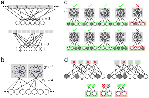
Figure 4: Architecture of the robust exponential ACAM. (a) Two bipartite networks, each with $N$ input neurons (bottom layer, circles) and $N_{C}$ constraint nodes (top layer, squares). The out-degree for the input nodes is set to $z=3$ in both networks. The top network exhibits excellent expansion: subsets of input nodes (one subset highlighted by dashed line) have many neighbors in the constraint layer. Equivalently, input neurons share relatively few common constraints. The network at bottom exhibits poor expansion: the same-sized subset of inputs has many fewer neighbors. (b) Each constraint node is a subnetwork of several sub-nodes or neurons. The number of neurons in the constraint node is $2^{z_{C}-1}$, where $z_{C}$ is the in-degree of the constraint node (a value that does not scale up with network size). Neurons in a constraint node receive global inhibition (hashed blue node). (c) Response of one constraint node to different configurations of its inputs. Each constraint neuron prefers one input configuration, determined by the weights from the inputs to that neuron (shown above a few neurons as a pattern of $+$’s and $-$’s): a positive (negative) weight from neuron $i$ causes the neuron to prefer input $i$ to be “on” (“off”); on (off) states are shown in white (gray). Here we have depicted all even-parity input states as the set of preferred states (green background). In a preferred input state, only one constraint neuron is strongly driven (white), corresponding to a low-energy or “satisfied” constraint (green check). For a non-preferred input (red background), multiple constraint neurons with preferred states that closely resemble the input are equally driven (white). Global inhibition forces no more than two of these constraint neurons to be active, and the constraint node wanders across configurations where pairs of these neurons are active. This is a higher-energy, unsatisfied constraint state (red cross). (d) Top left: network state with satisfied and unsatisfied constraints. An input attached to more unsatisfied than satisfied constraint nodes (red arrow, bottom) lowers the energy of the network when it flips, by flipping the status of all its constraint nodes (top right). Iteration of this process drives the network to the nearest Hamming-distance stable state. Bottom: Each constraint node is a weak check on its inputs: starting from a pair of satisfied constraints (left), corrupting a single input violates the constraints (center), but corrupting a second input (right) erases the signature of input error in the constraints. The problem of non-expansion: if two constraints have overlapping input states, they cannot help identify the source of input error (bottom center).

Self-organization to exponential capacity

We next show that a network with initially specified connectivity but unspecified weights can self-organize to have exponentially many well-separated minima. This self-organization can be performed by a simple one-shot learning rule that depends on the coactivation of pairs of input and constraint neurons. We start with a bipartite architecture consisting of $N$ input neurons in one layer and $N_{C}$ constraint nodes of $M$ neurons each in the other layer. An input neuron sends connections to $z$ randomly chosen constraint nodes, contacting all the neurons in the constraint node with weak non-specific connection strengths. Conversely, each neuron in a constraint node receives $z_{C}$ connections from input neurons, with all neurons in one constraint node connected to the same subset of inputs. We choose the number of neurons in a constraint node $M\geq 2^{z_{C}-1}$. Note that the degrees $z$ and $z_{C}$ do not need to be fixed (but we consider them fixed for simplicity).

During learning, we pair random sparse activation of constraint neurons with random patterns in the input neurons. When a constraint neuron is active, we set the weights of its connections to active input neurons to +1 and those to inactive input neurons to -1, in a Hebbian-like one-shot modification (Fig. 5a). We also set a background input to the constraint neurons so that all constraint neurons receive the same average input over time, regardless of their (learned) preferred input configurations. Once a synapse strength has been learned, it is no longer updated.

When a constraint neuron receives an input that matches or is close to (one input neuron flip away from) a previously seen and thus learned input, it will become active, suppressing the other constraint neurons in its node and preventing further learning. Consequently each constraint node learns to prefer a subset of possible input states that it sees, so long as they differ in at least two entries. This procedure is equivalent to each constraint node choosing a random subset of the presented input states, with a minimum Hamming distance of 2 between them (see SI, Section 11 for more details). As a whole, if the piece of an input pattern that one constraint sees is called a fragment, the network learns to prefer combinations of fragments from across all input patterns. Note that initially this process is greedy, with the network learning each presented fragment. However, later in the learning, presented fragments start to conflict with previously learned fragments (i.e., they differ in fewer than two entries), and the network ignores them.

As shown in Fig. 5b and c, this yields a network with a capacity (number of robust memory states) that grows exponentially with the number of neurons and the ability to recover from errors in a finite fraction of all neurons.

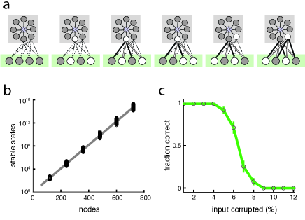
Figure 5: Input-driven self-organization of weights in a network with random connectivity. (a) Schematic of learning at a single constraint node. Initially the constraint node receives weak, non-specific projections from a subset of input nodes (first panel). Learning then proceeds by pairing random input patterns with sparse random activation of constraint neurons. If the input to a constraint node is not close to a previously learned pattern and a constraint neuron is active, the active constraint neuron learns connection strengths that prefer this pattern (second and third panels; fifth and sixth panels). If the constraint node receives an input that is close to a previously learned pattern, then the constraint neuron corresponding to this pattern activates and suppresses the activation of other constraint neurons (fourth panel). (b) Average number of fixed points for learned network. (c) Error-correction performance for learned network with N=480.

Robust retrieval of labels for noisy input patterns

As we describe in the Introduction (also see Discussion), it is impossible for a network with $N$ neurons to store more than $O(N)$ arbitrary patterns as memories. The patterns stored in our exponential capacity network are not arbitrary: they are determined by a large number of sparse constraints. Given these restrictions on the structure of patterns that can be stored at high capacity, how might these networks (or any such high capacity networks) be used?

One possibility is that the networks are used as content-addressable memories for a class of inputs with a particular structure, and we consider this possibility further in the Discussion.

Alternatively, the pre-structured repository of robust network memory states can serve as a neural pattern labeler (or locality-sensitive hash function), in which distributed input patterns are assigned abstract indices corresponding to the memory states, Fig. 6a,b. For example, some general theories of the hippocampus see it as assigning an index or hash value to sparse distributed patterns of cortical input ³⁹. However, for this to be possible with the relative sizes of cortex and the much-smaller hippocampus (the cortex in rats contains $10-100$ times more neurons than the hippocampus — $\sim 5\times 10^{7}$ in cortex versus $\sim 10^{6}$ in hippocampus ^{40; 41}, while in humans the factor is $\sim 1000$ — $\sim 10^{10}$ versus $\sim 10^{7}$ neurons^{42; 43; 41}) requires a high-capacity indexing scheme like the one we describe below.

Consider a set of $O(M)$ input patterns in a network with $M$ neurons, where $M$ is possibly very large. For example, cortical representations are typically sparse, and thus these input patterns could be a set of sparse cortical representations distributed across a large number of neurons. Or they might consist of non-sparse activity states lying on some low-dimensional subspace of the space of all patterns. We wish to map these input patterns to the (exponentially-many) stable states in a much smaller memory network. If the memory state has $N$ neurons, then $M$ can be $O(e^{N})$.

An appropriate feedforward mapping from the $M$-dimensional input network to the $N$-dimensional memory network can be constructed using a simple Hebbian or correlational learning rule that updates synaptic strengths using the product of the desired input and output states², numerical simulations in Fig. 6c and see SI S12 for proofs. Such a mechanism would require the memory network to be able to spontaneously move to new states to generate new labels (reminiscent of the observation that spontaneous plateau potentials in CA1 determine new place cells⁴⁴). Alternatively, if the set of input patterns are known ahead of time, the synapses for the feedforward mapping can be defined using a pseudoinverse construction; this produces a more noise-tolerant mapping than the Hebbian learning rule ¹⁴, as seen by contrasting the black and gray traces in Fig. 6c (and see SI S12). Either of these mappings involves $O(MN)$ total synapses (with $N<<M$); moreover, if the memory network is spatially-localized compared to the input network, then this scheme conserves wiring length compared to global connections in the input network.

If the input patterns are well-separated (as will be true for any generic set of $M$ patterns, see SI S12), then both the Hebbian and pseudoinverse mappings preserve the local neighborhood structure, in the sense that locally perturbed versions of an input pattern map to the local neighborhood of the corresponding label (SI S12). Thus, given a noisy input pattern within a neighborhood of the original, the state in the memory network flows to its stable state, retrieving the correct label (schematic in Figure 6a, numerical results in Fig. 6c and proofs in SI S12). The noise tolerance is linear in the dimension of the input space, meaning that it is possible for some finite fraction of the very large number of input neurons to be wrong. Consequently, the number of input errors can be much larger than the number of neurons in the memory network.

Thus, the memory network uses its exponential capacity to robustly index a much large number of input patterns. Note that this mapping is one-way: the labels can be recovered from the (possibly perturbed) input patterns but, in accordance with information-theoretic bounds ^{18; 19}, the labels cannot be used to recover the input pattern. Instead, the compressed labels generated and robustly retrieved by the exponential-capacity network in response to noisy or incomplete input patterns can then be used to drive downstream associations and actions using a much smaller number of synapses. Such a network could also be used for template matching, classification, locality-sensitive hashing and nearest neighbor computations (indeed, locality-sensitive hashing can be used to compute fast approximate nearest-neighbors⁴⁵), and for any computation where sparse patterns on a large space need to be compressed into dense patterns on a smaller space.

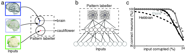
Figure 6: Robust labelling of input patterns. (a) Schematic of mapping input patterns from an $M=e^{N}$ dimensional input space to exponentially-many well-separated storage patterns in an $N$-dimensional network. (b) Structure of multi-layer network that carries out the mapping in (a). (c) Average number of errors in the input to the labelling network after feedforward mapping but before error correction in the labelling network (dashed line) and average number of errors after the network is allowed to perform error correction (solid line), both shown as a function of the number of flips in the M-dimensional input space. Here $M=10,000$, $N=480$ and number of stored patterns $=2000$. Black and gray traces show Hebbian and pseudoinverse constructions respectively.

Discussion

Unlike current theoretical neural architectures, which either show a small number of stable states (i.e. sub-exponential in network size) or weak error correction (i.e. the number of correctable errors is a vanishing fraction of network size), we demonstrate that neural networks with simple Hopfield dynamics can combine exponential capacity with robust error-correction. In the networks we construct, each constraint only weakly determines the state of the small number of nodes it is connected to: it restricts the states to a large subset of all possible states. However, the decorrelated structure of network connectivity, due to its expander graph architecture, means that these constraints are not strongly overlapping, and they can specify and correct patterns of errors on the inputs. In short, the network combines a large number of sparse, weak constraints near-optimally to produce systems with high capacity and robust error correction.

General arguments show that recurrent neural networks with $N$ neurons cannot store more than $O(N)$ arbitrary patterns as memories ^{18; 19}. A rough explanation of this limit is that fully-connected networks of $N$ neurons have $N^{2}$ synapses, which are the free parameters available for storing information. If each synapse has a finite dynamic range, the whole network contains $O(N^{2})$ bits of information (with a proportionality constant determined by the number of states at each synapse). An arbitrary binary pattern over $N$ neurons contains $N$ bits of information, therefore the network cannot store more than $O(N)$ such patterns. The networks we construct do not contradict these results even though the number of robust stable states is exponential: The patterns represented are not arbitrary. In other words, as with any super-linear capacity results ^{30; 31}, the networks we construct exhibit robust high-capacity storage for patterns with appropriate structure rather than for random patterns.

Is it possible to circumvent bounds on the storage of fully random patterns through an alternate scheme, in which exponentially many arbitrary patterns are mapped to these robust memory states? Encoders in communications theory do just this, mapping arbitrary inputs to well-separated states before transmission through a noisy channel. From a neural network perspective, the feedforward map can be viewed as a recurrent network with input and hidden units and asymmetric weights, so again we know from capacity results on non-symmetric weights ¹⁹ that it should not be possible. Mapping exponentially many arbitrary patterns to these structured memory states in a retrievable way would require specifying exponentially many pairings between inputs and structured memory states, and thus in general, equally many synapses. One way to obtain that many synapses would be to have exponentially many input neurons, but then the overall network would not possess exponential capacity for arbitrary many patterns as a function of network size. Note that this is the case for the neural pattern labeler we discuss above, where there are exponentially-many input neurons that are not part of the memory network, and thus the number of synapses required is smaller than the total squared network size. Put another way, while random projections of $\sim e^{M}$ points into an $M$ dimensional space preserve the relative distances and neighborhoods of these points ⁴⁶, which means that exponentially well-separated points can remain well-separated in a logarithmically shrunken dimensional space through a simple linear projection, such projections will not generally result in a specific expander structure of the embedding to allow for error correction by simple neural network dynamics. Arguably, however, brains are not built to store random patterns, and natural inputs that are stored well are not random.

As shown in Fig. 6, these networks can be used to to generate robust labels for arbitrary input patterns in a high-dimensional space. Another possible use for these networks is as content-addressable memories for inputs with appropriate structure. These inputs must be well-described as a product of a large number of sparse, weak, decorrelated constraints. For instance, natural images are generated from a number of latent causes or sources in the world, each imposing constraints on a sparse subset of the pixelated retinal data we receive. Alternatively, it must be possible to transform the set of inputs to have appropriate structure. For our networks, this would correspond to decorrelating structure in the lower moments of the data ^{47; 5; 48} while preserving structure in higher moments. It is still an open question what kinds of stimuli may either be naturally described within this framework or easily transformed to have the appropriate structure, but recent results suggest that the structure of natural images can be captured by the minima of Hopfield networks ⁸.

As observed by Sourlas ^{25; 49}, Hopfield networks and spin glasses can be viewed as error-correcting codes, with the stable states corresponding to codewords and the network dynamics corresponding to the decoding process. Moreover, it is possible to embed the codewords of general linear codes into the stable states of Hopfield networks with hidden nodes or higher-order connections (illustrated by our embedding of the Hamming code and shown in SI, Section 3) – thus, there can be exponentially many well-separated stable fixed points. However, decoding noisy inputs is a hard problem for high-capacity codes (decoding general linear codes is NP-hard ³⁴), requiring complex inference algorithms. These algorithms do not map naturally onto Hopfield dynamics, and as a result (as seen for the Hamming code) codewords cannot in general be correctly decoded by the internal dynamics of the neural network.

We leveraged here recent developments in high-dimensional graph theory and coding theory, on the construction of high-capacity low-density parity check codes (expander codes) that admit decoding by simple greedy algorithms ^{37; 38}, to show that ACAM networks with quasi-random connectivity can implement expander codes. If only pairwise connections are allowed then such a network requires hidden nodes. If higher-order connections are allowed then we show that sparse random ACAM networks (without hidden nodes) are isomorphic to expander codes (SI, Section 3) and generically have exponential capacity. Thus ACAM networks can have capacity and robustness performance comparable to state-of-the-art codes in communications theory, moreover with the decoder built into the dynamics.

For the case of Boltzmann dynamics, the network we construct is a Restricted Boltzmann Machine ^{50; 51} with constrained outdegree and inhibition (for sparsity) in the hidden layer. The network can be considered a product of experts ⁵¹, where each constraint node is an expert, and different neurons within a constraint node compete to enforce a particular configuration on their shared inputs. A constraint node as a whole constrains a small portion of the probability distribution.

Several recent ACAM network models are based on sparse bipartite graphs with stored states that occupy a linear subspace of all possible states ^{52; 53}. These networks exhibit exponential capacity for structured patterns, but either lack robust error correction ⁵³ or rely on complex non-neural dynamics with multiple stages ⁵².

The network of Hillar & Tran ³⁰ is notable in that it is close to exponential capacity, has large basins of attraction, shows very rapid convergence and is easy to construct. This network can also be understood in terms of a sparse constraint structure, with participation in a constraint determined by membership in the clique of an associated graph. These recent results suggest that sparse constraint structures can be leveraged in multiple ways to construct high capacity neural networks.

Expander graph neural networks leverage many weak constraints to provide near-optimal performance and exploit a property (i.e., expansion) that is rare in low dimensions but generic in high dimensions (and hence can be generated stochastically and without fine-tuning); both are common tropes in modern computer science and machine learning^{54; 55; 56; 57}, and expander graphs have found widespread recent use in designing algorithms^{35; 37}, including in solving challenging memory problems⁵⁸. Intriguingly, large sparse random networks are generically expander graphs ^{35; 36}, making such architectures promising for neural computation, where networks are large and sparse. The networks that we construct may thus provide broader insight into the computational capabilities of sparse, high-dimensional networks in the brain⁵⁹.

The network we construct has $N$ input/variable neurons and $N_{C}\sim N$ constraint nodes, each containing $2^{z_{c}-1}$ neurons. Thus this architecture has many more constraint cells than input cells. As a result, one key prediction of our model is that most cells are sparsely active, and their role is to impose constraints on network representations (this sparse strategy is feasible only in high dimensions/large networks, where exponential capacity on even a small fraction of the network can yield enough gains to outperform classical coding strategies). These constraint cells are only transiently active while they filter out irrelevant features, while cells that carry the actual representation will respond stably for a given state. Consequently, representations are predicted to contain a dense stable core, with many other neurons that are transiently active. This is reminiscent of observations in place cell population imaging ⁶⁰ and the sparse distribution of population activities across hippocampus and cortex ^{61; 62}. Neurons in each constraint node receive connections from the same subset of input neurons; this connection pattern resembles glomeruli, such as seen in the olfactory bulb and cerebellum ⁶³. On the other hand, the particular set of inputs to each constraint node are decorrelated or random, as required for good error correction. Thus the network architecture predicts clustered connections at the level of constraint neurons and, on the other hand, that input neurons should not share many of these constraint clusters in common. Finally, these architectures predict that representations in the input neurons should have relatively decorrelated second-order (i.e. pairwise) statistics, but should contain structure in higher-order moments that the network exploits for error correction.

In summary, we bridge neural network architectures and recent constructions in coding theory to construct a robust high-capacity neural memory system, and illustrate how sparse constraint structures with glomerular organization might provide a powerful framework for computation in large networks of neurons.

Methods

Hopfield networks and Boltzmann machines

We consider networks of $N$ binary nodes (the neurons). At a given time, $t$, each neuron has state $\boldsymbol{x}_{i}^{t}$=$0$ or $1$, corresponding to the neuron being inactive or active respectively. The network is defined by an $N$-dimensional vector of biases, $\boldsymbol{b}$, and an $N\times N$ symmetric weight matrix $W$. Here $\boldsymbol{b}_{i}$ is the bias (or background input) for the $i$th neuron (equivalently, the negative of the activation threshold), and $W_{ij}$ is the interaction strength between neurons $i$ and $j$ (set to 0 when $i=j$).

Neurons update their states asychronously according to the following rule:

$$\boldsymbol{x}_{i}^{t+1}=\begin{cases}1&\text{if }\sum_{j}W_{ij}\boldsymbol{x}_{j}^{t}+b_{i}>0\\ 0&\text{if}\sum_{j}W_{ij}\boldsymbol{x}_{j}^{t}+b_{i}<0\\ \text{Bern}(0.5)&\text{if}\sum_{j}W_{ij}\boldsymbol{x}_{j}^{t}+b_{i}=0\end{cases}$$ (5)

Here Bern(0.5) represents a random variable that takes values $0$ and $1$ with equal probability.

Hopfield networks can also be represented by an energy function, defined as

$$E(\boldsymbol{x}|\boldsymbol{\theta},W)=-\frac{1}{2}\sum_{i\neq j}W_{ij}\boldsymbol{x}_{i}\boldsymbol{x}_{j}-\sum_{i}\boldsymbol{b}_{i}\boldsymbol{x}_{i}$$ (6)

The dynamical rule is then to change the state of a neuron if doing so decreases the energy (and to change the state with $50\%$ probability if doing so leaves the energy unchanged).

We also consider Boltzmann machines, which are similar to Hopfield networks but have probabilistic update rules.

$$\boldsymbol{x}_{i}^{t+1} =\text{Bern}(p)$$

$$\text{where }p =\frac{1}{1+e^{-\beta(\sum_{j}W_{ij}\boldsymbol{x}_{j}^{t}-b_{i})}}$$ (7)

The probability of a state $\boldsymbol{x}$ in a Boltzmann machine is $p(\boldsymbol{x})\propto e^{-\beta E(\boldsymbol{x})}$, where $E(\boldsymbol{x})$ is defined as in Eq. 6 and $\beta$ is a scaling constant (often called inverse temperature). Note that the Hopfield network is the $\beta\rightarrow\infty$ limit of a Boltzmann machine.

Hopfield network implementation of Hamming code

The (7, 4) Hamming code can be defined on sets of 7 binary variables by the equations

$$x_{1}+x_{2}+x_{3}+x_{5} =0$$

$$x_{2}+x_{3}+x_{4}+x_{6} =0$$

$$x_{1}+x_{3}+x_{4}+x_{7} =0,$$ (8)

where all the sums are taken mod 2.

This is equivalent to a 4th-order Hopfield network with the energy function

$$E=-s_{1}s_{2}s_{3}s_{5}-s_{2}s_{3}s_{4}s_{6}-s_{1}s_{3}s_{4}s_{7}$$ (9)

Only here, for the sake of a tidy form for the energy function, we let the variables $s_{i}$ take values in $\{-1,+1\}$ rather than in $\{0,+1\}$ (it is straightforward to reexpress the energy function with $\{0,+1\}$ states, but the expression is less tidy). In the rest of this text, nodes take the values $\{0,+1\}$.

Hopfield network expander codes: construction

We consider a network with two layers: an input layer containing $N$ nodes that determine the states or memories that will be stored and corrected, and $N_{C}$ constraint modules that determine the permitted states of variables (see Figure 3). These constraint nodes are themselves small sub-networks of nodes (see below).

Each input neuron participates in $z$ constraints (i.e., is connected to $z$ constraint nodes), and each constraint node receives input from $z_{C}$ input neurons. Thus, the input neurons have degree $z$ and the constraint nodes have degree $z_{C}$; consequently $N\langle z\rangle=N_{C}\langle z_{C}\rangle$ (i.e., the number of edges leaving the input neurons equals the number of edges entering the constraint nodes). $z$ and $z_{C}$ are small (for Figure 3, $5\leq z\leq 10$ and $2\leq z_{C}\leq 6$, while for Figure 5, $z=5$ and $z_{C}=12$) and do not grow with the size of the network (i.e., with $N$ and $N_{C}$). Thus these networks are sparse.

The connections between the $N$ input neurons and the $N_{C}$ constraint nodes are chosen to be random, subject to the constraints on the degrees. Thus, with probability asymptotically approaching $1$ as $N$ increases, these networks are $(\gamma,(1-\epsilon))$ expanders with $\epsilon<1/4$ (see SI S5 and ^{37; 38}).

There are $z_{C}$ variables connected to a given constraint node and these could take any of $2^{z_{C}}$ possible states. The constraint nodes restrict this range, so that a subset of these states have low energy (and are thus preferred by the network). Each constraint node is actually a network of neurons with Hopfield dynamics and, while there are multiple possible ways to construct constraint nodes, in the construction that we show, each neuron in the constraint node prefers one possible configuration of the input neurons. For simplicity we choose these preferred states to be the parity states of the inputs (i.e. states where the sum of the inputs modulo 2 is 0), but note that the set of preferred states can be chosen quite generally (SI, Sections 6 and 9).

If a neuron in a constraint node prefers a particular state of its input neurons, then it has connection weights of +1 with the input neurons that are active in that state and weights of -1 with those that are inactive. Thus, a constraint neuron that prefers all of its input neurons to be on will receive an input of $z_{C}$ when its input is in the preferred state, and a constraint neuron that prefers only $k$ of these nodes to be active will receive input of $k$. To ensure that all constraint neuron receive the same amount of input in their preferred state, we also add biases of $z_{C}-k$ to each constraint node, where $k$ is the number of non-zero variables in its preferred state. Finally, to ensure that multiple constraint neurons are not simultaneously active during a preferred input for one sub-node, we add inhibitory connections of strength $z_{C}-1$ between all the sub-nodes in a constraint node. As a consequence of this strong inhibition, each constraint node has competitive dynamics: in the lowest energy state the input neurons are in a preferred configuration, the sub-node in the constraint node corresponding to this configuration is active, and all other sub-nodes are suppressed.

The network is in a stable or minimum energy state when all of the constraints are satisfied. As shown in Eqs. 2 and 3 in the main text, if the $j$th constraint node has $2^{z^{(j)}_{C}-r^{(j)}}$ permitted configurations (where $r^{(j)}\geq 1$ is some real number), then the network has an exponential number of minimum energy states.

Hopfield network expander codes: error correction

The proof that these networks can correct a constant fraction of errors is based on Sipser & Spielman (1996) ³⁷ and Luby et al. (2001) ³⁸ with slight generalization. We leave the details of the proof to the Supplementary Information, and sketch the main steps here.

We consider a set of corrupted input neurons, $S$, with size $|S|<\gamma N$. Since all subsets of size $<\gamma N$ expand, we can show that $S$ is connected to a comparatively large set of constraints, which we call $T$. In order for $|T|$ to be large, it must contain a large number of constraint nodes that are only connected to one neuron in $S$ (i.e. the neurons in $S$ do not share many constraint nodes in common), which we call non-shared. Constraint nodes can detect one error, so the non-shared nodes will be unsatisfied. If the fraction of non-shared constraint nodes is high, then at least one neuron in $S$ must be connected to more unsatisfied than satisfied constraint nodes, and it is energetically favorable for it to change its state. Thus, there is always an input neuron that is driven to change its state, reducing the number of unsatisfied constraints.

However, this does not exclude the possibility that the wrong input neuron changes its state. The remaining step of the proof is to show that the number of corrupted input neurons is bounded by a constant times the number of unsatisfied constraints. Thus, driving the number of unsatisfied constraints down to $0$ (which can always be done, as per the previous paragraph) will eventually correct all corrupted neurons (as long as the initial number of unsatisfied constraints is low enough to preclude convergence to the wrong energy minimum).

References

- 1 Little, W. The existence of persistent states in the brain. Math. Biosci. 19, 101–120 (1974).
- 2 Hopfield, J. J. Neural networks and physical systems with emergent collective computational abilities. Proc. Natl. Acad. Sci. U. S. A. 79, 2554–8 (1982).
- 3 Grossberg, S. Nonlinear neural networks: Principles, mechanisms, and architectures. Neural Netw. 1, 17–61 (1988).
- 4 Hinton, G. E. & Sejnowski, T. J. Optimal perceptual inference. In Proc. CVPR IEEE, 448–453 (Citeseer, 1983).
- 5 Olshausen, B. A. & Field, D. J. Emergence of simple-cell receptive field properties by learning a sparse code for natural images. Nature 381, 607–609 (1996).
- 6 Tishby, N., Pereira, F. C. & Bialek, W. The information bottleneck method. In Proceedings of the 37th Annual Allerton Conference on Communication, Control and Computing, 368–377 (1999).
- 7 Hinton, G. E. & Salakhutdinov, R. R. Reducing the dimensionality of data with neural networks. Science 313, 504–507 (2006).
- 8 Hillar, C., Mehta, R. & Koepsell, K. A Hopfield recurrent neural network trained on natural images performs state-of-the-art image compression. In IEEE Image Proc., 4092–4096 (IEEE, 2014).
- 9 LeCun, Y., Bengio, Y. & Hinton, G. Deep learning. Nature 521, 436–444 (2015).
- 10 McEliece, R. J., Rodemich, E. R., Rumsey Jr, H. & Welch, L. R. New upper bounds on the rate of a code via the Delsarte-MacWilliams inequalities. IEEE T. Inform. Theory 23, 157–166 (1977).
- 11 MacKay, D. Information Theory, Inference, and Learning Algorithms (Cambridge University Press, 2004).
- 12 McEliece, R., Posner, E. C., Rodemich, E. R. & Venkatesh, S. The capacity of the Hopfield associative memory. IEEE Trans. Inf. Theory 33, 461–482 (1987).
- 13 Amit, D. J., Gutfreund, H. & Sompolinsky, H. Storing infinite numbers of patterns in a spin-glass model of neural networks. Phys. Rev. Lett. 55, 1530 (1985).
- 14 Kanter, I. & Sompolinsky, H. Associative recall of memory without errors. Phys. Rev. A 35, 380 (1987).
- 15 Tsodyks, M. V. Associative memory in asymmetric diluted network with low level of activity. Europhys. Lett. 7, 203–208 (1988). URL Tsodyks88.pdf.
- 16 Hillar, C., Sohl-Dickstein, J. & Koepsell, K. Efficient and optimal binary hopfield associative memory storage using minimum probability flow. arXiv preprint arXiv:1204.2916 (2012).
- 17 Alemi, A., Baldassi, C., Brunel, N. & Zecchina, R. A three-threshold learning rule approaches the maximal capacity of recurrent neural networks. PLoS Comp. Biol. 11, e1004439 (2015).
- 18 Abu-Mostafa, Y. S. & St Jacques, J. Information capacity of the Hopfield model. IEEE Trans. Inf. Theory 31, 461–464 (1985).
- 19 Gardner, E. & Derrida, B. Optimal storage properties of neural network models. J. Phys. A 21, 271 (1988).
- 20 Treves, A. & Rolls, E. T. What determines the capacity of autoassociative memories in the brain? Network: Comp. Neural 2, 371–397 (1991).
- 21 Baldi, P. & Venkatesh, S. S. Number of stable points for spin-glasses and neural networks of higher orders. Phys. Rev. Lett. 58, 913 (1987).
- 22 Burshtein, D. Long-term attraction in higher order neural networks. IEEE Trans. Neural Netw. 9, 42–50 (1998).
- 23 Tanaka, F. & Edwards, S. Analytic theory of the ground state properties of a spin glass. I. ising spin glass. J. Phys. F 10, 2769 (1980).
- 24 McEliece, R. & Posner, E. The number of stable points of an infinite-range spin glass memory. Telecommunications and Data Acquisition Progress Report 42, 83 (1985).
- 25 Sourlas, N. Spin-glass models as error-correcting codes. Nature 339, 693–695 (1989).
- 26 Hopfield, J. J. & Tank, D. W. “Neural” computation of decisions in optimization problems. Biol. Cybern. 52, 141–152 (1985).
- 27 Hopfield, J. J. & Tank, D. W. Computing with neural circuits- a model. Science 233, 625–633 (1986).
- 28 Tank, D. W. & Hopfield, J. J. Simple ‘neural’ optimization networks: An A/D converter, signal decision circuit, and a linear programming circuit. IEEE Trans. Circuits Syst. 33, 533–541 (1986).
- 29 Alemi, A. & Abbara, A. Exponential capacity in an autoencoder neural network with a hidden layer. arXiv preprint arXiv:1705.07441 (2017).
- 30 Hillar, C. & Tran, N. M. Robust exponential memory in Hopfield networks. arXiv preprint arXiv:1411.4625 (2014).
- 31 Fiete, I., Schwab, D. J. & Tran, N. M. A binary Hopfield network with information rate and applications to grid cell decoding. arXiv preprint arXiv:1407.6029 (2014).
- 32 Shannon, C. A mathematical theory of communication. Bell Syst. Tech. J. 27, 379–423, 623–656 (1948).
- 33 Hamming, R. W. Error detecting and error correcting codes. Bell Syst. Tech. J. 29, 147–160 (1950).
- 34 Berlekamp, E. R., McEliece, R. J. & Van Tilborg, H. C. On the inherent intractability of certain coding problems. IEEE Trans. Inf. Theory 24, 384–386 (1978).
- 35 Hoory, S., Linial, N. & Wigderson, A. Expander graphs and their applications. Bull. Am. Math. Soc. 43, 439–561 (2006).
- 36 Lubotzky, A. Expander graphs in pure and applied mathematics. Bull. Am. Math. Soc. 49, 113–162 (2012).
- 37 Sipser, M. & Spielman, D. A. Expander codes. IEEE Trans. Inf. Theory 42, 1710–1722 (1996).
- 38 Luby, M. G., Mitzenmacher, M., Shokrollahi, M. A. & Spielman, D. A. Improved low-density parity-check codes using irregular graphs. IEEE Trans. Inf. Theory 47, 585–598 (2001).
- 39 Valiant, L. G. The hippocampus as a stable memory allocator for cortex. Neural Comput. 24, 2873–2899 (2012).
- 40 West, M., Slomianka, L. & Gundersen, H. J. G. Unbiased stereological estimation of the total number of neurons in the subdivisions of the rat hippocampus using the optical fractionator. Anat. Rec. 231, 482–497 (1991).
- 41 Herculano-Houzel, S. The human brain in numbers: a linearly scaled-up primate brain. Front. Hum. Neurosci. 3 (2009).
- 42 West, M. J. & Gundersen, H. Unbiased stereological estimation of the number of neurons in the human hippocampus. J. Comp. Neurol. 296, 1–22 (1990).
- 43 Pakkenberg, B. & Gundersen, H. J. G. Neocortical neuron number in humans: effect of sex and age. J. Comp. Neurol. 384, 312–320 (1997).
- 44 Bittner, K. C. et al. Conjunctive input processing drives feature selectivity in hippocampal ca1 neurons. Nat. Neuro. 18, 1133–1142 (2015).
- 45 Andoni, A. & Indyk, P. Near-optimal hashing algorithms for approximate nearest neighbor in high dimensions. In FOCS, 459–468 (IEEE, 2006).
- 46 Johnson, W. B. & Lindenstrauss, J. Extensions of Lipschitz mappings into a Hilbert space. Contemp. Math. 26, 1 (1984).
- 47 Barlow, H. B. Possible principles underlying the transformations of sensory messages. In Sensory Communication (MIT press, 1961).
- 48 Vinje, W. E. & Gallant, J. L. Sparse coding and decorrelation in primary visual cortex during natural vision. Science 287, 1273–1276 (2000).
- 49 Sourlas, N. Statistical mechanics and capacity-approaching error-correcting codes. Physica A 302, 14–21 (2001).
- 50 Smolensky, P. Information processing in dynamical systems: Foundations of harmony theory. In Parallel distributed processing: Explorations in the microstructure of cognition, 194––281 (MIT press, 1986).
- 51 Hinton, G. E. Training products of experts by minimizing contrastive divergence. Neural Comput. 14, 1771–1800 (2002).
- 52 Karbasi, A., Salavati, A. H. & Shokrollahi, A. Iterative learning and denoising in convolutional neural associative memories. In ICML (1), 445–453 (2013).
- 53 Salavati, A. H., Kumar, K. R. & Shokrollahi, A. Nonbinary associative memory with exponential pattern retrieval capacity and iterative learning. IEEE Trans. Neural Netw. Learn. Syst. 25, 557–570 (2014).
- 54 Candes, E. J., Romberg, J. K. & Tao, T. Stable signal recovery from incomplete and inaccurate measurements. Comm. Pure Appl. Math. 59, 1207–1223 (2006).
- 55 Donoho, D. L. Compressed sensing. IEEE Trans. Inf. Theory 52, 1289–1306 (2006).
- 56 Kuncheva, L. I. Combining pattern classifiers: methods and algorithms (John Wiley & Sons, 2004).
- 57 Schapire, R. E. The strength of weak learnability. Mach. Learn. 5, 197–227 (1990).
- 58 Larsen, K. G., Nelson, J., Nguyên, H. L. & Thorup, M. Heavy hitters via cluster-preserving clustering. In FOCS, 61–70 (IEEE, 2016).
- 59 Litwin-Kumar, A., Harris, K. D., Axel, R., Sompolinsky, H. & Abbott, L. Optimal degrees of synaptic connectivity. Neuron 93, 1153–1164 (2017).
- 60 Ziv, Y. et al. Long-term dynamics of CA1 hippocampal place codes. Nat. Neurosci. 16, 264–266 (2013).
- 61 Buzsáki, G. & Mizuseki, K. The log-dynamic brain: how skewed distributions affect network operations. Nat. Rev. Neuro. 15, 264–278 (2014).
- 62 Rich, P. D., Liaw, H.-P. & Lee, A. K. Large environments reveal the statistical structure governing hippocampal representations. Science 345, 814–817 (2014).
- 63 Shepherd, G. & Grillner, S. Handbook of brain microcircuits (Oxford University Press, 2010).