Stochastic gravitational wave background from newly born massive magnetars: The role of a dense matter equation of state

Abstract

Newly born massive magnetars are generally considered to be produced by binary neutron star (NS) mergers, which could give rise to short gamma-ray bursts (SGRBs). The strong magnetic fields and fast rotation of these magnetars make them promising sources for gravitational wave (GW) detection using ground based GW interferometers. Based on the observed masses of Galactic NS-NS binaries, by assuming different equations of state (EOSs) of dense matter, we investigate the stochastic gravitational wave background (SGWB) produced by an ensemble of newly born massive magnetars. The massive magnetar formation rate is estimated through: (i) the SGRB formation rate (hereafter entitled as MFR1); (ii) the NS-NS merger rate (hereafter entitled as MFR2). We find that for massive magnetars with masses $M_{\rm mg}=2.4743M_{\odot}$, if EOS CDDM2 is assumed, the resultant SGWBs may be detected by the future Einstein Telescope (ET) even for MFR1 with minimal local formation rate, and for MFR2 with a local merger rate $\dot{\rho}_{\rm c}^{\rm o}(0)\lesssim 10$ ${\rm Mpc}^{-3}{\rm Myr}^{-1}$. However, if EOS BSk21 is assumed, the SGWB may be detectable by the ET for MFR1 with the maximal local formation rate. Moreover, the background spectra show cutoffs at about 350 Hz in the case of EOS BSk21, and at 124 Hz for CDDM2, respectively. We suggest that if the cutoff at $\sim 100$ Hz in the background spectrum from massive magnetars could be detected, then the quark star EOS CDDM2 seems to be favorable. Moreover, the EOSs, which present relatively small TOV maximum masses, would be excluded.

I INTRODUCTION

Short gamma-ray bursts (SGRBs) are generally considered to be arising from the coalescence of either a neutron star-neutron star (NS-NS) binary or a neutron star-black hole (NS-BH) binary (see Berger:2014 for a recent review). Mergers of these compact binaries produce strong gravitational wave (GW) emissions, making them promising sources for GW detection using the ground based GW interferometers such as LIGO, VIRGO, GEO600, advanced LIGO (aLIGO), and the future Einstein Telescope (ET) Abbott:2009 ; Sath:2009 . The merger product of a NS-BH binary is of course a stellar-mass BH. On the other hand, the remnant of a NS-NS merger is still an open question. Depending on the total mass of the binary system and the NS equation of state (EOS), the NS-NS merger product may be either of the following four possibilities Rezzolla:2010 ; Lasky:2014 ; Ravi:2014 ; Gao:2016 : (1) a stellar-mass BH; (2) a differential rotation supported unstable hypermassive NS, which will collapse into a BH in a few tens milliseconds; (3) a centrifugal force supported temporarily stable massive NS, which will collapse into a BH when the NS is spun down; (4) an eternally stable massive NS. The massive NS remnants are suggested to possess strong surface dipole and internal toroidal magnetic fields, which are amplified due to various mechanisms, such as Kelvin-Helmholtz instability Anderson:2008 , magnetorotational instability Duez:2006 during/after the merger, $\alpha-\omegaup$ dynamo in the nascent millisecond NS Duncan:1992 , and the combined effect of r-mode and Tayler instabilities Cheng:2014 . Observationally, the existence of extended emissions Metzger:2008 , x-ray flares Campana:2006 , and internal x-ray plateaus Rowlinson:2013 in a large sample of SGRBs x-ray lightcurves support the idea that the central object of some SGRBs could be a highly magnetized, millisecond rotating NS.

Strong GW emission is expected in the final inspiral process of a NS-NS binary. Moreover, if the merger product is either (3) or (4), the remnant can also produce strong long-lasting GW signals, though their strengths may be relatively weak. Generally, the fast rotating, massive NS can emit GWs because of nonaxisymmetric instabilities, e.g., dynamical bar-mode instability Lai:1995 , r-mode instability Andersson:1998 , f-mode instability Andersson:1996 . On the other hand, strong internal magnetic fields of the massive magnetar can lead to nonaxisymmetric quadrupole deformation, which could also produce GW emission Bonazzola:1996 ; Stella:2005 ; Dall:2009 ; Dall:2015 . The amplitude of the magnetically induced GW signal is proportional to the quadrupole ellipticity Bonazzola:1996 , which mainly depends on the EOS, the magnetic energy, and the interior magnetic field configuration of the NS (see, e.g. Bonazzola:1996 ; Dall:2009 ; Gualtieri:2011 ; Haskell:2008 ; Cutler:2002 ; Ciolfi:2009 ; Mastrano:2011 ; Akgun:2013 ; Mastrano:2013 ; Mastrano:2015 ).

Superposition of the magnetically induced GW emissions from an ensemble of magnetars throughout the Universe can contribute to the astrophysical stochastic GW background (SGWB). The SGWB from the magnetic deformation of newly born magnetars has been discussed in many literature references Regimbau:2006 ; Marassi:2011 ; Rosado:2012 ; Cheng:2015 . However, in these papers, the magnetar mass is assumed to be a canonical value of $1.4M_{\odot}$, which means these magnetars are eternally stable. Actually, the magnetars produced by NS-NS mergers apparently have masses much larger than $1.4M_{\odot}$, and they may not be always stable [e.g., product (3) mentioned above]. For a single source, the collapse of the magnetar will lead to the cease of GW emission at a certain frequency. Hence, in order to derive a realistic SGWB produced by the magnetic deformation of newly born massive magnetars, both the EOS of dense matter and the masses of magnetars should be taken into account. In this paper, we reconsider the SGWB produced by magnetic deformation of the newly born, massive magnetars based on typical NS and quark star (QS) EOSs, and the observed masses of the Galactic NS-NS binaries. The motivation of considering the QS EOS is the recent statistical analysis of internal x-ray plateaus of SGRBs that shows that QS remnants might be more preferred than NSs Li:2016 . The paper is organized as follows: in Sec. II, we show how the GW signal from a single newly born massive magnetar is affected by the EOS. In Sec. III, we estimate the massive magnetar formation rate (MMFR) based on two different results: (i) the SGRB rate at redshift $z$ suggested in Yonetoku:2014 ; (ii) the NS-NS merger rate as predicted by Regimbau and Hughes Regimbau:2009 . Results for the SGWBs produced by an ensemble of newly born massive magnetars are shown in Sect. IV. Conclusion and discussions are presented in Sect. V.

II GW EMISSION FROM THE NEWLY BORN MASSIVE MAGNETAR

We assume that all SGRBs are produced by NS-NS mergers, and the merger remnants are either temporarily or eternally stable massive NSs/QSs. Generally, in the merger process, only $\lesssim 10^{-2}M_{\odot}$ materials are ejected from the NS-NS binary system Hotokezaka:2013 . Hence, the total rest mass of the system is basically conserved, e.g., $M_{\rm r,m}=M_{\rm r,1}+M_{\rm r,2}$, where $M_{\rm r,m}$ represents the rest mass of the massive magnetar remnant, $M_{\rm r,1}$ and $M_{\rm r,2}$ are the rest masses of the two NSs, respectively. Based on the approximate relation Timmes:1996 between rest and gravitational masses, by assuming that the extragalactic NS-NS binaries have the same gravitational mass distribution as the Galactic NS-NS binary population, one can easily estimate the distribution of gravitational mass $M_{\rm mg}$ for the massive magnetar remnants Lasky:2014 ; Ravi:2014 ; Gao:2016 ; Li:2016 .

Until now there are six Galactic NS-NS binaries that have a relatively accurate measured gravitational mass for each NS in the binary system; they are PSR J0737-3039 (with gravitational masses $M_{\rm g,1}=1.3381M_{\odot}$ and $M_{\rm g,2}=1.2489M_{\odot}$ for the two NSs, respectively), PSR B1534+12 ($M_{\rm g,1}=1.3332M_{\odot}$ and $M_{\rm g,2}=1.3452M_{\odot}$), PSR B1913+16 ($M_{\rm g,1}=1.4398M_{\odot}$ and $M_{\rm g,2}=1.3886M_{\odot}$), PSR B2127+11C ($M_{\rm g,1}=1.358M_{\odot}$ and $M_{\rm g,2}=1.354M_{\odot}$), PSR J1906+0746 ($M_{\rm g,1}=1.248M_{\odot}$ and $M_{\rm g,2}=1.365M_{\odot}$), and PSR J1756-2251 ($M_{\rm g,1}=1.40M_{\odot}$ and $M_{\rm g,2}=1.18M_{\odot}$) Kiziltan:2013 . Therefore, the gravitational mass of the massive magnetar remnant is $2.4046M_{\odot}$ as inferred from the binary system PSR J0737-3039, $2.4845M_{\odot}$ inferred from PSR B1534+12, $2.6154M_{\odot}$ inferred from PSR B1913+16, $2.5139M_{\odot}$ inferred from PSR B2127+11C, $2.4276M_{\odot}$ inferred from PSR J1906+0746, $2.3996M_{\odot}$ inferred from PSR J1756-2251. The average gravitational mass of the massive magnetars is thus $M_{\rm mg}=2.4743M_{\odot}$, and we take this value as the typical mass for the massive magnetars in the remainder of this paper.

For a nonrotating NS/QS, the maximum gravitational mass that it could sustain is the Tolman-Oppenheimer-Volkoff (TOV) maximum mass, $M_{\rm TOV}$, which is determined by the NS/QS EOSs. However, centrifugal forces due to the uniform rotation of the merger remnant could increase the maximum sustainable gravitational mass. Li et al. Li:2016 calculated equilibrium sequences of uniformly rotating NS/QS configurations with a spin frequency increasing from 0 to the Keplerian spin limit and obtained analytical expressions for the maximum gravitational mass $M_{\rm g,max}$, the corresponding equilibrium radius $R_{\rm eq}$ (in kilometers), and the corresponding maximum moment of inertia $I_{\rm max}$ of a NS/QS with a spin period $P$ (in milliseconds), which, respectively, have the following form:

$$M_{\rm g,max} = M_{\rm TOV}(1+\alpha P^{\beta});$$ (1)

$$R_{\rm eq} = C+AP^{B};$$ (2)

$$I_{\rm max} = M_{\rm g,max}R_{\rm eq}^{2}\frac{a}{1+e^{-k(P-q)}},$$ (3)

where $M_{\rm g,max}$ and $M_{\rm TOV}$ are measured in solar masses. The fitting parameters $\alpha$, $\beta$, $A$, $B$, $C$, $a$, $q$, and $k$ are EOS dependent. For the typical NS (BSk21 Potekhin:2013 ) and QS (CDDM2 Chu:2014 ) EOSs considered in this paper, the specific values of these parameters as well as $M_{\rm TOV}$ can be found in Table 1 of Li:2016 .

From Eq. (1), one can define the collapse frequency, $\nu_{\rm coll}=1/P_{\rm coll}$, below which the massive magnetar with a gravitational mass $M_{\rm mg}=M_{\rm g,max}(P_{\rm coll})$ will immediately collapse into a BH. The specific form of $\nu_{\rm coll}$ is Lasky:2014 ; Ravi:2014 ; Gao:2016

$$\nu_{\rm coll}=\left({\alpha M_{\rm TOV}\over M_{\rm mg}-M_{\rm TOV}}\right)^{1/\beta}.$$ (4)

If $\nu_{\rm coll}\leq 0$ (i.e., $M_{\rm mg}\leq M_{\rm TOV}$), the massive magnetar is eternally stable. However, if $0<\nu_{\rm coll}<\nu_{\rm i}$ (with $\nu_{\rm i}$ represents the initial spin frequency), the massive magnetar is temporarily stable, and it will collapse into a BH when the star spins down to $\nu_{\rm coll}$ due to GW emission and magnetic dipole radiation (MDR). Lastly, if $\nu_{\rm coll}>\nu_{\rm i}$, the massive magnetar will collapse into a BH immediately after it is born. Remarkable GW emissions from the central remnant are expected only in the first two cases (i.e., eternally stable and temporarily stable magnetars). For the EOSs BSk21 and CDDM2 considered here, the massive magnetar remnant with an initial spin at the Keplerian limit should be temporarily stable because $0<\nu_{\rm coll}<\nu_{\rm i}$ (see below). Other EOSs that provide $M_{\rm TOV}>2.4743M_{\odot}$ will result in an eternally stable massive magnetar, and continuous GW emission extended to lower frequencies.

The newly born massive magnetar spins down mainly through MDR and magnetically induced GW emission. Therefore, the evolution formula for the angular frequency $\omega$ of the magnetar can be written as

$$\dot{\omega}=-\frac{B_{\rm d}^{2}R^{6}\omega^{3}}{6Ic^{3}}-\frac{32G\epsilon_{\rm B}^{2}I\omega^{5}}{5c^{5}},$$ (5)

where $B_{\rm d}$ is the surface dipole magnetic field at the magnetic pole, $R$ the radius, and $I$ the moment of inertia of star. By adopting different interior magnetic field configurations and stellar interior structures, the magnetically induced quadrupole ellipticity $\epsilon_{\rm B}$ has been calculated in many literature references (e.g., Bonazzola:1996 ; Haskell:2008 ; Dall:2009 ; Dall:2015 ; Cutler:2002 ; Ciolfi:2009 ; Gualtieri:2011 ; Mastrano:2011 ; Akgun:2013 ; Mastrano:2013 ; Mastrano:2015 ). Some nonlinear numerical simulations show that the interior magnetic field probably has a poloidal-toroidal twisted-torus shape Braithwaite:2004 . However, even for this configuration, the dominated one is usually the toroidal field component. In the toroidal-dominated case, $\epsilon_{\rm B}$ is related to the volume-averaged strength of the toroidal field ${\bar{B}}_{\rm t}$ Cutler:2002 , which is hard to be determined directly. Generally, ${\bar{B}}_{\rm t}/B_{\rm d}\approx 5$–$100$ with $B_{\rm d}$ the dipole magnetic field of the magnetar is proposed following the observations of giant flare from SGR 1806-20 Stella:2005 , free precession of magnetar 4U 0142+61 Makishima:2014 , x-ray afterglows of some SGRBs Fan:2013 , and lightcurves of superluminous supernovae Moriya:2016 . For a NS the ellipticity can be estimated as $\epsilon_{\rm B}\approx 10^{-4}({\bar{B}}_{\rm t}/10^{16}~{}{\rm G})^{2}$ Cutler:2002 ; Lasky:2016 . While for a QS, if it is in the two-flavor color superconductivity phase Alford:1998 , the ellipticity is approximated as $\epsilon_{\rm B}\approx 7\times 10^{-4}({\bar{B}}_{\rm t}/10^{16}~{}{\rm G})$ for the mass and radius adopted thereinafter Glampedakis:2012 . On the other hand, $\epsilon_{\rm B}$ can be constrained via analyzing the internal x-ray plateau afterglows of SGRBs Gao:2016 ; Li:2016 . Specifically, depending on the EOSs, the ellipticity of the massive magnetar is confined to be $\epsilon_{\rm B}=0.002$ for NS EOS BSk21 and $\epsilon_{\rm B}=0.004$–$0.007$ for QS EOS CDDM2 Li:2016 . Thereinafter, the representative ellipticities $\epsilon_{\rm B}=0.005$ (the value with the best Kolmogorov-Smirnov test), and $\epsilon_{\rm B}=0.002$ will be taken for EOSs CDDM2, and BSk21, respectively, while calculating the GW signal emitted by a single magnetar and the SGWB from the massive magnetar population Li:2016 . The corresponding strength of the toroidal field is thus ${\bar{B}}_{\rm t}\approx 4.5\times 10^{16}$ ($7.1\times 10^{16}$) G for a NS (QS).

The GW energy spectrum emitted by a single newly born massive magnetar can be estimated as

$$\frac{dE_{\rm GW}}{d\nu_{\rm e}}={32\pi G\over 5c^{5}}\epsilon_{\rm B}^{2}I^{2}\omega^{6}\left|\dot{\omega}^{-1}\right|,$$ (6)

where $\nu_{\rm e}=\omega/\pi$ is the GW frequency at the source frame. One can also obtain the characteristic amplitude of the emitted GW as follows Jaranowski:1998 ; Corsi:2009 :

$$h_{\rm c}(\nu_{\rm e})={\nu_{\rm e}h(t)\over\sqrt{d\nu_{\rm e}/dt}},$$ (7)

where $h(t)={4\pi^{2}GI\epsilon_{\rm B}\nu_{\rm e}^{2}\over c^{4}d}$ is the GW strain amplitude, $d$ is the distance to the source. To assess the detectability of the GW signal, we calculate the optimal (matched-filter) signal-to-noise ratio (SNR) as Corsi:2009

$${\rm S/N}=\left[\int_{\nu_{\rm e,min}}^{\nu_{\rm e,max}}\frac{h_{\rm c}^{2}}{\nu_{\rm e}^{2}S_{h}(\nu_{\rm e})}d\nu_{\rm e}\right]^{1/2},$$ (8)

where $\nu_{\rm e,min}$(=$2\nu_{\rm coll}$) and $\nu_{\rm e,max}$(=$2\nu_{\rm i}$) are, respectively, the minimum and maximum GW frequencies emitted by the magnetar, $S_{h}(\nu_{\rm e})$ is the one-sided noise power spectral density of the detector. The analytical expressions of $S_{h}(\nu_{\rm e})$ can be found in Sathyaprakash:2009 for aLIGO and ET.

We do not follow instantaneous variations of the gravitational mass, radius, and moment of inertia with the spin-down of the massive magnetar, though all these quantities should actually decrease. For simplicity, we take a typical gravitational mass $M_{\rm mg}$, radius $R$, and moment of inertia $I$ for the massive magnetar and assume they do not evolve with time during spin-down. For a magnetar with $M_{\rm mg}=2.4743M_{\odot}$, its $R$ and $I$ are EOS dependent, which can be estimated as follows. The radius $R$ is approximately estimated by substituting the derived collapse period $P_{\rm coll}=1/\nu_{\rm coll}$ into Eq. (2). Then with $R$ and $P_{\rm coll}$, using Eq. (3), the moment of inertia $I$ can be obtained approximately. The resultant radius and moment of inertia of the $2.4743M_{\odot}$ magnetar are, respectively, $R=12.66$ (16.31) km and $I=3.68\times 10^{45}$ ($5.50\times 10^{45}$) ${\rm g~{}cm}^{2}$ if EOS BSk21 (CDDM2) is assumed. Obviously, $R$ and $I$ are underestimated for the $2.4743M_{\odot}$ magnetar that initially spins at the Keplerian limit $P_{\rm K}$. As a rough estimation, assuming a constant mass $M_{\rm mg}=2.4743M_{\odot}$, the ratio between the magnetar radii obtained at $P_{\rm K}$ and at $P_{\rm coll}$ is $R(P_{\rm K})/R(P_{\rm coll})\approx 1.1$ (1.4) for EOS BSk20 (CDDM1) (see Fig. 1 of Li:2016 ). Furthermore, with the spin-down of the magnetar, $R(P)/R(P_{\rm coll})$ should decrease and become equal to 1 when $P_{\rm coll}$ is reached, where $R(P)$ denotes the instantaneous radius of the magnetar with a spin period $P$. For EOSs BSk21 and CDDM2 considered, $R(P_{\rm K})/R(P_{\rm coll})$ are not expected to vary too much from the above values. Following Eqs. (7) and (6), we have $h_{\rm c}\propto R$, and $dE_{\rm GW}/d\nu_{\rm e}\propto R^{2}$ during the early period of spin-down when the GW emission is dominant. Consequently, our choice of a constant $R$ will at most underestimate the characteristic amplitude $h_{\rm c}$, and the background emission $\Omega_{\rm GW}$ [see Eq. (14)] by a factor of 1.4 and 2, respectively. Hence, it is reasonable to take a constant $R$ and $I$ for a specific EOS in the calculations below.

Following Li et al. Li:2016 , the dipole magnetic field of the massive magnetar is taken to be $B_{\rm d}=10^{15}$ G, and the initial angular frequency is taken as $\omega_{\rm i}=2\pi/P_{\rm K}$. The values of $P_{\rm K}$ for EOSs BSk21 and CDDM2 can be found in Li:2016 . Assuming EOSs BSk21 and CDDM2, we show the characteristic amplitude $h_{\rm c}$ of the GW signal versus the emitted frequency $\nu_{\rm e}$ in Fig. 1. The distance to the source is taken to be $d=100$ Mpc. The massive magnetar with $M_{\rm mg}=2.4743M_{\odot}$ is temporarily stable for EOSs BSk21 and CDDM2, and it will not collapse until $\nu_{\rm coll}$ is reached. The collapse of the magnetar is manifested as a catastrophic cutoff in the emitted GW signal at $2\nu_{\rm coll}$, which is about 2453 Hz for EOS BSk21, and 868 Hz for EOS CDDM2, as shown in Fig. 1. For EOS BSk21, the GW signal emitted by the massive magnetar extends from about 3322 Hz down to 2453 Hz. While for EOS CDDM2, the emitted GW is at lower frequency band, which covers the range from 1778 to 868 Hz.

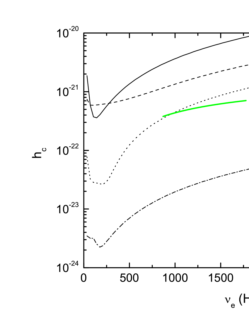
Figure 1: The GW characteristic amplitude $h_{\rm c}$ versus the emitted frequency $\nu_{\rm e}$, calculated by assuming NS EOS BSk21 (red line) and QS EOS CDDM2 (green line). For comparison, the rms strain noises for LIGO (solid line), VIRGO (dashed line), aLIGO (dotted line), and the future ET (dash-dotted line) are also presented Sathyaprakash:2009 .

Since the strength of ${\bar{B}}_{\rm t}$ of a newly born magnetar is highly uncertain, in order to comprehensively show how ${\bar{B}}_{\rm t}$ could affect the detectability of GW signal from a single source, in Fig. 2, the SNR S/N is plotted as a function of ${\bar{B}}_{\rm t}$, whose range is $\sim 5$–$100B_{\rm d}$ as discussed above. Obviously, with the increase of ${\bar{B}}_{\rm t}$, the SNR is gradually enhanced. However, for different EOSs, the evolution behaviors of S/N with ${\bar{B}}_{\rm t}$ differ significantly. Compared with EOS CDDM2, as ${\bar{B}}_{\rm t}$ increases, S/N shows a more obvious trend of getting saturated when EOS BSk21 is assumed. This is because for NS EOS BSk21, the ellipticity is more sensitive to the increase of ${\bar{B}}_{\rm t}$ ($\epsilon_{\rm B}\propto{\bar{B}}_{\rm t}^{2}$ versus $\epsilon_{\rm B}\propto{\bar{B}}_{\rm t}$ for QS EOS CDDM2). When $\epsilon_{\rm B}$ is large enough, GW emission will dominate the spin-down; thus, we have ${\rm S/N}\propto h(t)/\sqrt{d\nu_{\rm e}/dt}={\rm const}$. Moreover, using the same detector, the derived SNR is higher for EOS CDDM2, since the sensitivities of the detectors are better at a relatively low frequency band. Assuming EOS BSk21, the SNRs of the GW emitted by the magnetar with a representative ellipticity $\epsilon_{\rm B}=0.002$ are 4.18 for ET (red filled star in Fig. 2) and 0.17 for aLIGO (red hollow star). While assuming EOS CDDM2 and $\epsilon_{\rm B}=0.005$, we have S/N=16.65 for ET (green filled star in Fig. 2) and S/N=0.72 for aLIGO (green hollow star). Adopting a single-detector search, the detection threshold is roughly S/N=8 Abadie:2010 . Hence, using ET, the emitted GW by the $2.4743M_{\odot}$ magnetar at $100$ Mpc is undetectable if EOS BSk21 is assumed even for ${\bar{B}}_{\rm t}=10^{17}$ G. For comparison, when EOS CDDM2 is assumed, a detectable GW signal is expected if ${\bar{B}}_{\rm t}\gtrsim 2.3\times 10^{16}$ G (see Fig. 2), which may easily be achieved for newly born magnetars. Consequently, if future ET could detect the GW emitted by the $2.4743M_{\odot}$ magnetar, then QS EOS CDDM2 will be more preferred. Moreover, observation of the cutoff in the GW signal using ET may provide us an important channel to distinguish different EOSs.

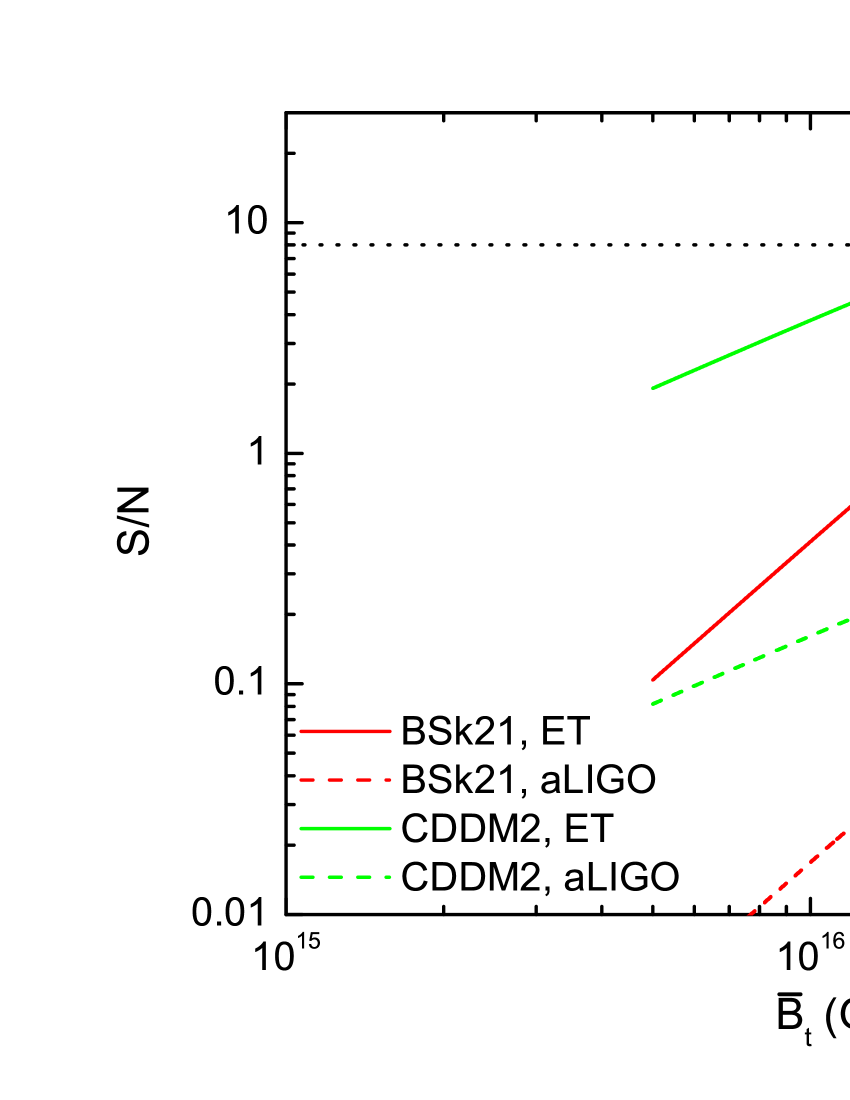
Figure 2: The SNR S/N of the GW signal emitted by a single massive magnetar versus the magnetar’s interior toroidal magnetic field ${\bar{B}}_{\rm t}$. The SNRs are calculated by assuming NS EOS BSk21 (red lines), and QS EOS CDDM2 (green lines), respectively. The solid lines represent the SNRs obtained using future ET, while the dashed lines show the results derived using aLIGO. The dotted line indicates the detection threshold for a single-detector search. The stars show the SNRs calculated by adopting various representative ellipticities and for different detectors (see the text).

III THE MASSIVE MAGNETAR FORMATION RATE

As a quite rough estimation, the MMFR can be considered to be equal to the formation rate of SGRBs because we have assumed that only NS-NS mergers produce SGRBs and the merger products can only be temporarily stable or eternally stable massive magnetars. Obviously, this assumption will lead to an overestimation of the MMFR. Using the spectral peak energy-peak luminosity correlation for SGRBs, Yonetoku et al. Yonetoku:2014 determined the redshifts of 72 BATSE SGRBs and obtained the relation between the SGRB formation rate and the redshift, which has the following form:

$$\rho_{\rm SGRB}(z)=\left\{\begin{aligned} &\rho_{\rm SGRB}(0)(1+z)^{6}&,~{}~{}&0<z<0.67&\\ &\rho_{\rm SGRB}(0)\times 1.67^{6}&,~{}~{}&z\geq 0.67&\end{aligned}\right.,$$ (9)

where $\rho_{\rm SGRB}(0)$ is the local SGRB formation rate. Hereafter, we refer to this as magnetar formation rate 1 (MFR1) and assume that the MMFR can be described by Eq. (9) up to $z_{\ast}\sim 6$. The minimum SGRB formation rate at $z=0$ is estimated to be $\rho_{\rm SGRB,min}(0)=1.15\times 10^{-7}$ events ${\rm Mpc}^{-3}{\rm yr}^{-1}$ by involving the geometrical correction of beaming angles Yonetoku:2014 . On the other hand, using the peak fluxes of 14 Swift SGRBs, redshifts, and beaming angles inferred from x-ray observations, Coward et al. Coward:2012 obtained an upper limit for the local formation rate as $\rho_{\rm SGRB,max}(0)=1.1\times 10^{-6}$ events ${\rm Mpc}^{-3}{\rm yr}^{-1}$ in the case of beamed emission.

To estimate the MMFR, one can also equivalently estimate the NS-NS merger rate under the assumption that NS-NS mergers can only produce temporarily stable or eternally stable massive magnetars. Hereafter, we refer to the MMFR derived in this way as magnetar formation rate 2 (MFR2). Assuming that the NS-NS merger rate tracks the cosmic star formation rate (CSFR) with the time delay $t_{\rm d}$ from formation of the NS binary to the final merger, the observed NS-NS merger rate at redshift $z$ can be written as Regimbau:2009

$$\dot{\rho}_{\rm c}^{\rm o}(z)=\dot{\rho}_{\rm c}^{\rm o}(0)\times\frac{\dot{\rho}_{\rm\ast,c}(z)}{\dot{\rho}_{\rm\ast,c}(0)},$$ (10)

where $\dot{\rho}_{\rm c}^{\rm o}(0)$ is the observed local merger rate per unit volume, whose value can be extrapolated by multiplying the Galactic NS-NS merger rate with the density of Milky Way-like galaxies. Following Regimbau and Hughes Regimbau:2009 , we take two representative values for the local merger rate: (i) $\dot{\rho}_{\rm c}^{\rm o}(0)=10$ ${\rm Mpc}^{-3}{\rm Myr}^{-1}$, which is the upper limit of the local merger rate; (ii) $\dot{\rho}_{\rm c}^{\rm o}(0)=1$ ${\rm Mpc}^{-3}{\rm Myr}^{-1}$, which represents the most probable value for the rate. The NS-NS merger rate is related to the CSFR by the quantity $\dot{\rho}_{\rm\ast,c}(z)$, which can be given as Regimbau:2009

$$\dot{\rho}_{\rm\ast,c}(z)=\int\frac{\dot{\rho}_{\rm\ast}(z_{\rm f})}{1+z_{\rm f}}P(t_{\rm d})dt_{\rm d},$$ (11)

where $\dot{\rho}_{\rm\ast}$ is the CSFR. $z$ and $z_{\rm f}$ are the redshifts at which the NS-NS binary mergers and its progenitor binary initially formed, respectively. $t_{\rm d}$ is the time difference between the formation of the progenitor binary and the compact binary, plus the merging time of the binary. It also represents the lookback time between $z$ and $z_{\rm f}$, which has an approximate form $t_{\rm d}\simeq{2\over 3H_{\rm 0}}(1/\sqrt{\Omega_{m}(1+z)^{3}+\Omega_{\Lambda}}-1/\sqrt{\Omega_{m}(1+z_{\rm f})^{3}+\Omega_{\Lambda}})$. In this paper, the $\Lambda$CDM cosmological model is taken with the Hubble constant $H_{\rm 0}=70~{}{\rm km~{}s}^{-1}{\rm Mpc}^{-1}$, $\Omega_{m}=0.3$, and $\Omega_{\Lambda}=0.7$. Based on the result of population synthesis (see Regimbau:2009 and references therein), the probability distribution $P(t_{\rm d})$ for the time delay $t_{\rm d}$ is given by

$$P(t_{\rm d})\propto 1/t_{\rm d}~{}~{}{\rm with}~{}~{}t_{\rm d}>\tau_{0},$$ (12)

for some minimal delay time $\tau_{0}$. For NS-NS binary, the minimal delay time is assumed to be $\tau_{0}=20$ Myr, which corresponds to the evolution time from massive binaries to NS-NS binaries Regimbau:2009 .

For the CSFR, we use the result suggested in Hopkins and Beacom Hopkins:2006 . Based on the new measurements of the galaxy luminosity function in the UV and far-infrared wavelengths, they refined the previous models up to $z_{\ast}\sim 6$ and obtained a parametric fit formula for the CSFR, which takes the following form Hopkins:2006 :

$$\dot{\rho}_{\rm\ast}(z)=h\frac{0.017+0.13z}{1+(z/3.3)^{5.3}}M_{\odot}{\rm yr}^{-1}{\rm Mpc}^{-3},$$ (13)

where $h=0.7$.

IV RESULTS

The SGWB is generally represented by the dimensionless quantity, $\Omega_{\rm GW}(\nu_{\rm obs})$, which describes the distribution of the GW energy density versus the GW frequency in the observer frame $\nu_{\rm obs}$. The SGWB produced by the magnetic deformation of an ensemble of newly born massive magnetars is given by Regimbau:2006 ; Marassi:2011 ; Cheng:2015

$$\Omega_{\rm GW}(\nu_{\rm obs})=\frac{8\pi G\nu_{\rm obs}}{3H_{0}^{3}c^{2}}\int_{z_{\rm low}}^{z_{\rm upp}}\frac{\rho_{\rm MFR}(z)}{(1+z)E(\Omega,z)}\frac{dE_{\rm GW}}{d\nu_{\rm e}}dz,$$ (14)

where $\nu_{\rm obs}=\nu_{\rm e}/(1+z)$, $E(\Omega,z)=\sqrt{\Omega_{m}(1+z)^{3}+\Omega_{\Lambda}}$, and $\rho_{\rm MFR}(z)$ is the MMFR, which can be substituted by Eqs. (9) or (10). $z_{\rm upp}$ and the $z_{\rm low}$ are the upper and lower limits of the redshift integration, respectively. $z_{\rm upp}$ depends on the maximal redshift $z_{\ast}$ of the MMFR model and the maximal value of $\nu_{\rm e}$, i.e., $z_{\rm upp}=$min$(z_{\ast},\nu_{\rm e,max}/\nu_{\rm obs}-1)$. While $z_{\rm low}$ is determined by the minimal value of $\nu_{\rm e}$, i.e., $z_{\rm low}=$max$(0,\nu_{\rm e,min}/\nu_{\rm obs}-1)$.

The optimal SNR of the background emission for an observation time $T$ is given as Allen:1999

$$({\rm S/N})_{\rm B}=\left[\frac{9H_{0}^{4}T}{50\pi^{4}}\int_{0}^{\infty}\frac{\gamma^{2}(\nu_{\rm obs})\Omega_{\rm GW}^{2}(\nu_{\rm obs})}{\nu_{\rm obs}^{6}S_{h1}(\nu_{\rm obs})S_{h2}(\nu_{\rm obs})}d\nu_{\rm obs}\right]^{1/2},$$ (15)

where $S_{h1}(\nu_{\rm obs})$, $S_{h2}(\nu_{\rm obs})$ are the noise power spectral densities of the two detectors, and $\gamma$ is the normalized overlap reduction function. For two colocated and coaligned detectors, $\gamma=1$, and we simply assume $S_{h1}(\nu_{\rm obs})=S_{h2}(\nu_{\rm obs})$.

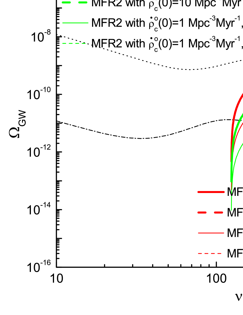
Figure 3: Dimensionless GW energy density $\Omega_{\rm GW}$ versus the observational frequency $\nu_{\rm obs}$, calculated for different MMFR models with various local formation rates and different EOSs as shown in the legend. The newly born massive magnetars have $M_{\rm mg}=2.4743M_{\odot}$, and $B_{\rm d}=10^{15}$ G. Other quantities for the magnetars are taken to be EOS dependent (see the text). For comparison, the detection thresholds of aLIGO (black dotted line) and the future ET (black dash-dotted line) calculated following Eq. (136) in Sathyaprakash:2009 and assuming a 1 yr observation time are also shown.

By considering different MMFR models (MFR1 and MFR2) and EOSs (BSk21 and CDDM2), in Fig. 3, we plot the SGWBs contributed by an ensemble of newly born massive magnetars with $M_{\rm mg}=2.4743M_{\odot}$. As mentioned before, depending on the EOS, the radii, representative ellipticities, and initial spin frequencies of magnetars are taken to be $R=12.66$ (16.31) km, $\epsilon_{\rm B}=0.002$ (0.005), and $\nu_{\rm i}=1660.85$ (888.97) Hz for EOS BSk21 (CDDM2), while the dipole magnetic fields are taken the same as $B_{\rm d}=10^{15}$ G for all magnetars Li:2016 . Consequently, the maximal observed GW frequency is $\nu_{\rm obs}^{\rm max}\simeq 3322$ Hz for EOS BSk21 and 1778 Hz for EOS CDDM2. For the same EOS, the background spectra calculated by using MFR1 have different shapes in comparison with those derived by using MFR2. For instance, the peak frequencies are at 830$-$1690 Hz for MFR1 versus 1132$-$2455 Hz for MFR2. Moreover, assuming EOS CDDM2, the spectrum calculated based on MFR1 with $\rho_{\rm SGRB}(0)=1.1\times 10^{-6}$ events ${\rm Mpc}^{-3}{\rm yr}^{-1}$ (red thick solid line) dominates the spectrum obtained by using MFR2 with $\dot{\rho}_{\rm c}^{\rm o}(0)=10$ ${\rm Mpc}^{-3}{\rm Myr}^{-1}$ (green thick solid line) at $\nu_{\rm obs}\lesssim 1200$ Hz, however, succumbs to the later above 1200 Hz. This is because MFR1 predicts higher $\rho_{\rm MFR}(z)$ at high $z$, but lower $\rho_{\rm MFR}(z)$ at low $z$. The source formation rate at high (low) $z$ mainly contributes to background emission at low (high) frequency band Zhu:2011 .

It is obvious that the background spectra are strongly dependent on the assumed EOSs as shown in Fig. 3. The EOS BSk21 leads to a cutoff at $\nu_{\rm e}\simeq 2453$ Hz in the GW signal emitted by a single magnetar with $M_{\rm mg}=2.4743M_{\odot}$ (see Fig. 1). Such cutoffs also appear in the background spectra emitted by an ensemble of such magnetars if EOS BSk21 is assumed. However, the observed cutoff frequency depends on the maximal redshift of the MMFR model as $\nu_{\rm cut}=2453/(z_{\ast}+1)\simeq 350$ Hz with $z_{\ast}=6$ for the two MMFR models. In contrast, using a commonly assumed mass $1.4M_{\odot}$ for newly born magnetars, the resultant background spectrum extends down to several hertz without a cutoff because these magnetars do not collapse Regimbau:2006 ; Marassi:2011 ; Rosado:2012 ; Cheng:2015 . With EOS BSk21, the background emissions cover the frequency band from 2453 to 350 Hz, which are not in the sensitive band of ET. The background spectrum may only be detected by ET in the case of MFR1 with $\rho_{\rm SGRB}(0)=1.1\times 10^{-6}$ events ${\rm Mpc}^{-3}{\rm yr}^{-1}$ (red thick dashed line in Fig. 3). The corresponding SNR of the background spectrum is $(\rm S/N)_{\rm B}=3.38$ (red hollow star in Fig. 4) for ET when an observation time $T=1$ yr is assumed. The SNR is slightly above the detection threshold $(\rm S/N)_{\rm B,th}=2.56$ of ET (dotted line in Fig. 4) Marassi:2011 . A lower SNR with $(\rm S/N)_{\rm B}=0.69$ (green hollow star in Fig. 4) is obtained using MFR2 with $\dot{\rho}_{\rm c}^{\rm o}(0)=10$ ${\rm Mpc}^{-3}{\rm Myr}^{-1}$. Consequently, it should be hard to confirm EOS BSk21 through direct observation of such a cutoff in the background spectrum emitted by massive magnetars.

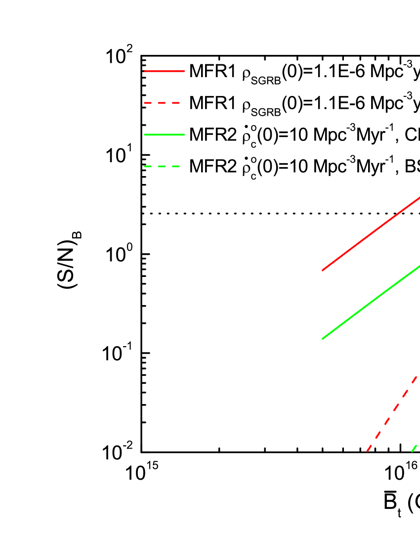
Figure 4: The SNR $(\rm S/N)_{\rm B}$ of SGWB from a massive magnetar population versus the magnetars’ interior toroidal magnetic fields ${\bar{B}}_{\rm t}$. The SNRs are calculated by assuming different EOSs and various MMFRs as depicted in the legend. All SNRs are derived with respect to ET for an observation time of 1 yr. The dotted line shows the detection threshold of ET. The stars represent the SNRs calculated by adopting various representative ellipticities (corresponding to various EOSs) and for different MMFRs (see the text).

As a comparison, if the EOS CDDM2 is assumed, the resultant background spectra emitted by all magnetars with $M_{\rm mg}=2.4743M_{\odot}$ show cutoffs at $\nu_{\rm cut}\simeq 124$ Hz. The spectra extend from 1778 Hz down to 124 Hz. Using ET and taking $T=1$ yr, the SNR of the background spectrum is 50.49 (red filled star in Fig. 4) for MFR1 with $\rho_{\rm SGRB}(0)=1.1\times 10^{-6}$ events ${\rm Mpc}^{-3}{\rm yr}^{-1}$. The SNR is reduced by about an order of magnitude for the minimal local SGRB formation rate $\rho_{\rm SGRB,min}(0)=1.15\times 10^{-7}$ events ${\rm Mpc}^{-3}{\rm yr}^{-1}$. Moreover, adopting MFR2 with $\dot{\rho}_{\rm c}^{\rm o}(0)=10$ ${\rm Mpc}^{-3}{\rm Myr}^{-1}$, the resultant SNR is 10.28 for ET (green filled star in Fig. 4). The SNRs are all above the detection threshold of ET, which suggest that the spectra may be detectable by the proposed ET. If the cutoff at $\sim 100$ Hz in the SGWB from massive magnetars could be detected in the future, then the EOS of dense matter may be consistent with QS EOS CDDM2. Furthermore, the EOSs (e.g., BSk21 and APR) which provide relatively small $M_{\rm TOV}$ could be excluded. Of course, the nondetection of the background emission may have the following reasons: (i) the actual $\rho_{\rm MFR}(z)$ is much smaller than those we adopted here; (ii) the EOSs (e.g., BSk21 and APR) which provide relatively small $M_{\rm TOV}$ are favorable; (iii) the magnetars actually have much lower ${\bar{B}}_{\rm t}$.

Related to the last point of the above reasons, the effect of ${\bar{B}}_{\rm t}$ on the detection of the SGWB is shown in Fig. 4. All the SNRs of the background emissions are calculated by adopting the maximal local event rate of each MMFR model, an observation time $T=1$ yr, and with respect to ET, which has the best designed sensitivity. In all cases, as ${\bar{B}}_{\rm t}$ increases, the SNR of the background first rises rapidly then slowly. Specially, the same as in Fig. 2, when EOS BSk21 is assumed the SNR of the background tends to be saturated when ${\bar{B}}_{\rm t}$ becomes large enough. In this case, even MFR1 with $\rho_{\rm SGRB}(0)=1.1\times 10^{-6}$ events ${\rm Mpc}^{-3}{\rm yr}^{-1}$ and the maximal toroidal fields ${\bar{B}}_{\rm t}\sim 10^{17}$ G are taken, $(\rm S/N)_{\rm B}$ is slightly above detection threshold of ET. This just reflects that the background emission from massive magnetars is difficult to be detected if EOSs with small $M_{\rm TOV}$ are preferred as discussed above. In contrast, for the same MMFR and ${\bar{B}}_{\rm t}$, $(\rm S/N)_{\rm B}$ derived based on EOS CDDM2 is at least $\sim 10$ times higher than that obtained by assuming EOS BSk21 (see Fig. 4). Hence, if EOS CDDM2 rather than EOS BSk21 is preferred, detection of the background emission from massive magnetars may be promising.

The SGWB produced by an ensemble of massive magnetars is expected to be continuous if the duty cycle $DC=\int_{0}^{6}\tau(1+z)\rho_{\rm MFR}(z)dV\gg 1$ is satisfied Coward:2006 . The quantity $\tau$ is the duration of the GW signal emitted by a single magnetar. The expression for the comoving volume element $dV$ can be found in Zhu:2011 . In the case of EOS BSk21, since the $2.4743M_{\odot}$ massive magnetar has a dipole field $B_{\rm d}=10^{15}$ G and representative ellipticity $\epsilon_{\rm B}=0.002$, its lifetime can be determined to be $\tau=140.50$ s. The massive magnetar has a much longer lifetime of $\tau=995.86$ s if EOS CDDM2 is assumed, even though its representative ellipticity ($\epsilon_{\rm B}=0.005$) is larger in this case. Using MFR2 with $\dot{\rho}_{\rm c}^{\rm o}(0)=1$ ${\rm Mpc}^{-3}{\rm Myr}^{-1}$ (the lowest MMFR), we have $DC\simeq 39.02$ (276.56) for EOS BSk21 (CDDM2), which means that the SGWB from these magnetars is continuous. We note that even when EOS BSk21 and ultrastrong toroidal fields ${\bar{B}}_{\rm t}\sim 10^{17}$ G are assumed for the massive magnetars, the produced SGWB is still continuous if the MMFR is not as low as MFR2 with $\dot{\rho}_{\rm c}^{\rm o}(0)=1$ ${\rm Mpc}^{-3}{\rm Myr}^{-1}$.

V CONCLUSION AND DISCUSSIONS

As one of the most promising targets for GW detection, newly born magnetars, if produced by NS-NS mergers, their masses should be much larger than the generally assumed value $1.4M_{\odot}$ for NSs. The masses of the newly born magnetars, the EOSs, and the MMFR models all have an impact on the SGWB produced by the massive magnetar population. By taking into account these effects, we estimated the SGWB produced by the newly born massive magnetars. For the NS EOS BSk21 and QS EOS CDDM2 adopted here, the resultant background spectra contributed by massive magnetars with $M_{\rm mg}=2.4743M_{\odot}$ show cutoffs at about 350 Hz, and 124 Hz, respectively. The frequency ranges of background emissions are different for the two EOSs. Assuming EOS CDDM2 and representative ellipticities $\epsilon_{\rm B}=0.005$ for the $2.4743M_{\odot}$ massive magnetars, even using MFR1 with the minimal local rate, the SGWB contributed by an ensemble of such magnetars may be detected by the future ET. While using MFR2, the background emission from these magnetars may be detected by ET only if the local merger rate satisfies $\dot{\rho}_{\rm c}^{\rm o}(0)\lesssim 10$ ${\rm Mpc}^{-3}{\rm Myr}^{-1}$. However, if EOS BSk21 (and representative ellipticities $\epsilon_{\rm B}=0.002$) is assumed, the SGWB may be detected by ET only when MFR1 with the maximal local rate is adopted. For the same MMFR and ${\bar{B}}_{\rm t}$, adopting EOS CDDM2, the SNR of the background is at least $\sim 10$ times higher than that obtained based on EOS BSk21. This, in turn, may indicate that if such background emission could be detected, EOS CDDM2 should be more favorable. The relatively low SNR of the background emission indicates that it may be unlikely to test EOS BSk21 via detecting the cutoff in the background spectrum. However, if the cutoff at $\sim 100$ Hz in the SGWB from massive magnetars could be detected in the future, the QS EOS CDDM2 seems to be favorable. In addition, successful detection of background emission at $\gtrsim 100$ Hz could reasonably exclude the EOSs which present relatively small $M_{\rm TOV}$ (e.g., EOSs BSk21 and APR). Finally, detecting the GW emission during the entire formation process (from the final binary inspiral process to the magnetar phase) of a newly born massive magnetar may still be an effective way to probe the EOS of dense matter because one need not estimate the MMFR, which is actually rather uncertain.

Improvements are still needed in order to obtain a more realistic SGWB produced by an ensemble of massive magnetars. In this paper, we only assume typical mass $M_{\rm mg}=2.4743M_{\odot}$ for the massive magnetars. Actually, the masses of these massive magnetars should distribute in a certain range as inferred from the mass distribution of Galactic NS-NS binaries Kiziltan:2013 . In future work, we will combine the mass distribution of massive magnetars with various NS/QS EOSs to study the SGWB produced by the massive magnetars in detail.

- (1) Berger, E. 2014, ARA&A, 52, 43; Rosswog, S. 2015, IJMPD, 24, 1530012
- (2) Abbott, B. P., et al. 2009, Rep. Prog. Phys., 72, 076901;
- (3) Sathyaprakash, B. S., Schutz, B. F. 2009, Living Rev. Relativ., 12, 2
- (4) Rezzolla, L., et al. 2010, Classical and Quantum Gravity, 27, 114105
- (5) Lasky, P. D., et al. 2014, Phys. Rev. D, 89, 047302
- (6) Ravi, V., Lasky, P. D. 2014, MNRAS, 441, 2433
- (7) Gao, H., Zhang, B., Lü, H. J. 2016, Phys. Rev. D, 93, 044065
- (8) Anderson, M., et al. 2008, Phys. Rev. Lett., 100, 191101
- (9) Duez, M.D., Liu, Y. T., Shapiro, S. L., Shibata, M., Stephens, B. C. 2006, Phys. Rev. D, 73, 104015
- (10) Duncan, R. C., Thompson, C. 1992, ApJ, 392, L9
- (11) Cheng, Q., Yu, Y. W. 2014, ApJL, 786, L13
- (12) Metzger, B. D., Quataert, E., Thompson, T. A. 2008, MNRAS, 385, 1455
- (13) Campana, S., et al. 2006, A&A, 454, 113
- (14) Rowlinson, A., et al. 2013, MNRAS, 430, 1061
- (15) Lai, D., Shapiro, S. L. 1995, ApJ, 442, 259
- (16) Andersson, N. 1998, ApJ, 502, 708; Friedman, J. L., Morsink, S. M. 1998, ApJ, 502, 714
- (17) Andersson, N., Kokkotas, K. D. 1996, Phys. Rev. Lett., 77, 4134; Kokkotas, K. D., Apostolatos, T. A., Andersson, N. 2001, MNRAS, 320, 307; Passamonti, A., Gaertig, E., Kokkotas, K. D., Doneva, D. 2013, Phys. Rev. D, 87, 084010; Doneva, D. D., Gaertig, E., Kokkotas, K. D., Krüger, C. 2013, Phys. Rev. D, 88, 044052; Doneva, D. D., Kokkotas, K. D., Pnigouras, P. 2015, Phys. Rev. D, 92, 104040
- (18) Bonazzola, S., Gourgoulhon, E. 1996, A&A, 312, 675
- (19) Stella, L., Dall Osso, S., Israel, G. L., Vecchio, A. 2005, ApJ, 634, L165
- (20) Dall’Osso, S., Shore, S. N., Stella, L. 2009, MNRAS, 398, 1869
- (21) Dall’Osso, S., Giacomazzo, B., Perna, R., Stella, L. 2015, ApJ, 798, 25
- (22) Haskell, B., Samuelsson, L., Glampedakis, K., Andersson, N. 2008, MNRAS, 385, 531;
- (23) Cutler, C. 2002, Phys. Rev. D, 66, 084025
- (24) Ciolfi, R., Ferrari, V., Gualtieri, L., Pons, J. A. 2009, MNRAS, 397, 913
- (25) Gualtieri, L., Ciolfi, R., Ferrari, V. 2011, Class. Quantum Grav., 28, 114014
- (26) Mastrano, A., Melatos, A., Reisenegger, A., Akgün, T. 2011, MNRAS, 417, 2288
- (27) Akgün, T., Reisenegger, A., Mastrano, A., Marchant, P. 2013, MNRAS, 433, 2445
- (28) Mastrano, A., Lasky, P. D., Melatos, A. 2013, MNRAS, 434, 1658
- (29) Mastrano, A., Suvorov, A. G., Melatos, A. 2015, MNRAS, 447, 3475
- (30) Regimbau, T., de Freitas Pacheco, J. A. 2006, A&A, 447, 1
- (31) Marassi, S., Ciolfi, R., Schneider, R., Stella, L., Ferrari, V. 2011, MNRAS, 411, 2549
- (32) Rosado, P. A. 2012, Phys.Rev. D, 86, 104007
- (33) Cheng, Q., Yu, Y. W., Zheng, X. P. 2015, MNRAS, 454, 2299
- (34) Li, A., Zhang, B., Zhang, N. B., Gao, H., Qi, B., Liu, T. 2016, Phys.Rev. D, 94, 083010
- (35) Yonetoku, D., Nakamura, T., Sawano, T., Takahashi, K., Toyanago, A. 2014, ApJ, 789, 65
- (36) Regimbau, T., Hughes, S. A. 2009, Phys.Rev. D, 79, 062002
- (37) Hotokezaka, K., et al. 2013, Phys. Rev. D, 87, 024001; Sekiguchi, Y., Kiuchi, K., Kyutoku, K., Shibata, M. 2015, Phys. Rev. D, 91, 064059; Palenzuela, C., et al. 2015, Phys. Rev. D, 92, 044045
- (38) Timmes, F. X., Woosley, S. E., Weaver, T. A. 1996, ApJ, 457, 834
- (39) Kiziltan, B., Kottas, A., De Yoreo, M., Thorsett, S. E. 2013, ApJ, 778, 66
- (40) Potekhin, A.-Y., Fantina, A.-F., Chamel, N., Pearson, J.-M., Goriely, S. 2013, A&A, 560, A48
- (41) Chu, P.-C., Chen, L.-W. 2014, ApJ, 780, 135
- (42) Braithwaite, J., Spruit, H. C. 2004, Nature, 431, 819; Braithwaite, J., Spruit, H. C. 2006, A&A, 450, 1097;
- (43) Makishima, K., Enoto, T., Hiraga, J. S., Nakano, T., Nakazawa, K., Sakurai, S., Sasano, M., Murakami, H. 2014, Phys. Rev. Lett., 112, 171102
- (44) Fan, Y. Z., Wu, X. F., Wei, D. M. 2013, Phys. Rev. D, 88, 067304
- (45) Moriya, T. J., Tauris, T. M. 2016, MNRAS, 460, L55
- (46) Lasky, P. D., Glampedakis, K. 2016, MNRAS, 458, 1660
- (47) Alford, M., Rajagopal, K., Wilczek, F. 1998, Phys. Lett. B, 422, 247
- (48) Madsen, J. 2000, Phys. Rev. Lett. 85, 10
- (49) Cheng, Q., Yu, Y. W., Zheng, X. P. 2013, Phys. Rev. D, 87, 063009
- (50) Glampedakis, K., Jones, D. I., Samuelsson, L. 2012, Phys. Rev. Lett., 109, 081103
- (51) Jaranowski, P., Królak, A., Schutz, B. F. 1998, Phys. Rev. D, 58, 063001
- (52) Corsi, A., Mészáros, P. 2009, ApJ, 702, 1171
- (53) Sathyaprakash, B. S., Schutz, B. F. 2009, Living Rev. Relativ., 12, 2
- (54) Abadie, J., Abbott, B. P., Abbott, R., et al. 2010, Classical and Quantum Gravity, 27, 173001
- (55) Coward, D. M., et al. 2012, MNRAS, 425, 2668
- (56) Hopkins, A. M., Beacom, J. F. 2006, ApJ, 651, 142
- (57) Allen, B., Romano, J. D. 1999, Phys. Rev. D, 59, 102001
- (58) Zhu, X. J., Fan, X. L., Zhu, Z. H. 2011, ApJ, 729, 59
- (59) Coward, D. M., Regimbau, T. 2006, New Astron. Rev., 50, 461