Optimizing Adiabatic Quantum Program Compilation using a Graph-Theoretic Framework

Abstract

Adiabatic quantum computing has evolved in recent years from a theoretical field into an immensely practical area, a change partially sparked by D-Wave System’s quantum annealing hardware. These multimillion-dollar quantum annealers offer the potential to solve optimization problems millions of times faster than classical heuristics, prompting researchers at Google, NASA and Lockheed Martin to study how these computers can be applied to complex real-world problems such as NASA rover missions. Unfortunately, compiling (embedding) an optimization problem into the annealing hardware is itself a difficult optimization problem and a major bottleneck currently preventing widespread adoption. Additionally, while finding a single embedding is difficult, no generalized method is known for tuning embeddings to use minimal hardware resources. To address these barriers, we introduce a graph-theoretic framework for developing structured embedding algorithms. Using this framework, we introduce a biclique virtual hardware layer to provide a simplified interface to the physical hardware. Additionally, we exploit bipartite structure in quantum programs using odd cycle transversal (OCT) decompositions. By coupling an OCT-based embedding algorithm with new, generalized reduction methods, we develop a new baseline for embedding a wide range of optimization problems into fault-free D-Wave annealing hardware. To encourage the reuse and extension of these techniques, we provide an implementation of the framework and embedding algorithms.

1 Introduction

Adiabatic quantum computing (AQC) is a model of computation that utilizes quantum mechanics to solve difficult optimization problems. As originally proposed by Farhi et al. farhi2000quantum , AQC relies on the dynamical evolution of a quantum state under a Hamiltonian that changes adiabatically from an initial to final form. This computational model uses the final Hamiltonian to express an optimization problem such that adiabatic evolution will recover the corresponding ground state.

In its most general form, the AQC model is equivalent to other universal quantum computing models. However, any limitation on the Hamiltonian forms may reduce the power of the computational model. Recently, an embodiment of the AQC model with a restricted Hamiltonian was developed using superconducting flux qubits by D-Wave Systems Inc. This quantum processor provides a large number of addressable qubits (up to 2048 in the latest D-Wave 2000Q processor) that implement a programmable Ising model over a restricted geometry. While not a universal quantum computer, the D-Wave processor has been shown to produce quantum effects and yield time-to-solution orders of magnitude faster than classical algorithms denchev2016what ; king2017quantum . Use of this quantum annealer kadowaki1998quantum has evolved beyond the design stage to testing and deployment, with recent applications including computational chemistry, NP-hard graph problems, image recognition, and more denchev2016what ; kassal2011simulating ; lucas2014ising ; neven2008image ; rieffel2015case ; venturelli2015quantum .

A key step in using current AQC-based processors is compiling the executable program that will run on hardware with restricted connectivity humble2014integrated ; britt2015high . Both the problem and hardware layouts are conventionally represented using graphs with the problem defined by variables connected with dependencies and the hardware layouts defined by qubits connected with couplers. Under this graph-theoretic formulation, the compilation process reduces to the NP-hard problem of minor embedding the problem graph into the hardware graph. In practice, this step represents a limitation bottleneck for the end-to-end program performance because existing embedding algorithms take orders of magnitude longer to execute than the quantum annealer itself humble2016performance . Furthermore, no efficient universal embedding algorithm exists, with past algorithms addressing specific classes of problem instance (e.g. complete graphs, very sparse graphs, etc.) and hardware instance (e.g. D-Wave Chimera graph, etc.), along with a myriad of additional assumptions (e.g. fault-free hardware, parameter values, etc.). However, given the disjoint development of algorithms for these specialized instances, the resulting techniques cannot be combined in a common framework.

To address this incompatibility, we introduce a graph-theoretic framework for developing tuned and modularized embedding algorithms. This framework introduces the concept of a virtual hardware graph that provides a judiciously simplified representation of the physical hardware graph, greatly reducing the complexity of embedding subroutines. Many existing embedding algorithms are compatible with the virtual hardware layer and we rewrite them as modular subroutines. We then introduce generalized reduction subroutines for minimizing the hardware footprint of a given embedding. We are able to apply these reduction subroutines to the embedding algorithms emulated by our framework, producing notable improvements for reducing hardware footprint.

As a proof of concept, we provide a complete bipartite virtual hardware compatible with the D-Wave Chimera hardware structure. By exploiting bipartite problem structure with an odd cycle transversal decomposition (OCT), we are able to provide embeddings for edge-dense problem graphs. We additionally present a linear-time approximation algorithm for computing OCT decompositions, leading to fast embedding algorithms. Further use cases are provided by Hamilton and Humble hamilton2016identifying .

Finally, we provide an efficient implementation of the full virtual hardware framework, including new and existing embedding and reduction subroutines, available at https://github.com/TheoryInPractice/aqc-virtual-embedding. Experimentally, we find that this framework is able to unify and expand on existing embedding algorithms, providing baseline tools for future development. Further, we find that OCT-based embedding algorithms perform better – in run time, size of problem graph embedded, and number of qubits used – than the existing TRIAD and CMR algorithms cai2014practical ; choi2011minor .

The manuscript is organized as follows: Section 2 introduces adiabatic quantum computing and the D-Wave hardware, including an overview of related work. Section 3 defines virtual hardware and a stack of baseline subroutines – the graph-theoretic framework – and details the emulation and enhancement of existing embedding algorithms using our framework. Section 4 introduces a new embedding subroutine that exploits bipartite structure in problem and hardware graphs by using an odd cycle transversal decomposition and biclique virtual hardware, respectively; we additionally present a new, fast approximation algorithm for computing an odd cycle transversal. Section 5 contains experimental results of embedding algorithms detailed in previous sections. Finally, we summarize, present our conclusions, and outline future work in Section 6.

2 Background

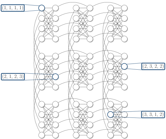
Figure 1: A Chimera $\mathcal{C}_{3,3,4}$ graph. The Chimera location labels of four qubits are highlighted.

We assume graphs are simple and undirected. For a graph $G$, we denote its vertices with $V(G)$ and edges with $E(G)$, and let $n=|V(G)|$ and $m=|E(G)|$ if the graph in question is clear from the context. Given a set of vertices $S$, we use $G[S]$ to denote the subgraph induced by $S$, and $G\setminus S$ to denote $G[V(G)-S]$. We denote the complete graph on $n$ vertices as $K_{n}$ and the complete bipartite graph on $n=n_{1}+n_{2}$ vertices with partite sets of order $n_{1},n_{2}$ as $K_{n_{1},n_{2}}$. As shorthand, we also refer to complete bipartite graphs as bicliques. We denote the neighbors of a vertex $u$ as $N(u)$. An edge $(u,v)$ can be contracted by adding a vertex $uv$ with incident edges to the vertices $N(u)\cup N(v)$, and then deleting $u$ and $v$. We also define the contraction of a connected subgraph $H$ as the iterative contraction of its edges (order does not matter due to connectivity). For a set $S$ we denote its power set as $\mathcal{P}(S)$.

Current and prior D-Wave hardware layouts are based on the more general Chimera graphs. Visualized in Fig. 1, a Chimera graph $\mathcal{C}_{L,M,N}$ is an $M\times N$ grid of biclique $K_{L,L}$ cells. For example, the latest D-Wave 2000Q hardware is based on a $\mathcal{C}_{4,16,16}$ graph. In the context of Chimera hardware, we assume that the qubits are labeled by their location in the Chimera layout: $(\ell_{r},\ell_{c},\ell_{p},\ell_{h})$ where $1\leq\ell_{r}\leq M$ identifies a row, $1\leq\ell_{c}\leq N$ identifies a column, $\ell_{p}\in\{1,2\}$ identifies a partite set, and $1\leq\ell_{h}\leq L$ denotes the in-cell height index.

2.1 Minor Embedding for Adiabatic Quantum Programming

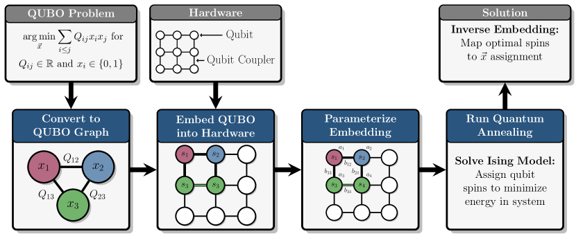
Figure 2: A typical workflow for running QUBO-formulated optimization problems on an AQC processing unit. Finding efficient and effective embedding algorithms is an area of active research.

Programming a quantum annealer, such as the D-Wave hardware, requires setting the parameters that define the underlying Ising Model. This process includes defining the positive and negative spins as variable assignments such that logical dependencies are maintained within the restricted connectivity of the hardware graph. Recently, several efficient compilation methods have been proposed for managing this process choi2008minor ; humble2014integrated ; rieffel2015case ; venturelli2015quantum .

A generalized compilation pipeline is shown in Fig. 2. A common entry point into these compilation frameworks is the quadratic unconstrained binary optimization (QUBO) problem. Given variables $x_{1},\dots,x_{n}$ where $x_{i}\in\{0,1\}$ and constants $c_{ij}\in\mathbb{R}$, the QUBO problem is to compute

$$\operatorname*{arg\,min}\sum_{i\leq j}c_{ij}x_{i}x_{j}.$$

QUBO has become a standard input format for quantum annealers, similar to the linear program format used in efficient classical solvers such as CPLEX. Many constrained optimization problems can be converted directly to QUBO form boros2002pseudo .

A QUBO can be converted directly into a graph $P$ with vertices $V(P)=\{x_{1},\dots,x_{n}\}$, edges $E(P)=\{(x_{i},x_{j})~{}|~{}i\neq j,c_{ij}\neq 0\}$, vertex weights $c_{ii}$, and edge weights $c_{ij}$ for $i\neq j$. Viewing a QUBO as a graph is particularly useful when selecting sets of physical qubits to represent the QUBO variables, since this assignment is known as graph minor embedding:

Definition 1 (Minor Embedding)

Given two graphs $P$ and $H$, a minor embedding of $P$ into $H$ is a function $\phi:V(P)\to\mathcal{P}(V(H))$ that assigns each vertex in $P$ to a vertex set from $V(H)$ such that the following properties hold:

1. Vertex sets cannot overlap: $\phi(u)\cap\phi(v)=\emptyset$ for all distinct $u,v\in V(P)$.

2. Vertex sets induce connected subgraphs: $H[\phi(u)]$ is connected for every $u\in V(P)$.

3. Edges are represented: $(u,v)\in E(P)\to(u^{\prime},v^{\prime})\in E(H)$ for some $u^{\prime}\in\phi(u)$ and $v^{\prime}\in\phi(v)$.

From a graph-theoretic perspective, this embedding defines the vertex deletions and edge contractions necessary to find $P$ as a minor of $H$. From the physics perspective, this embedding assigns an appropriate set of physical qubits to collectively represent a logical qubit, and QUBO weights are adjusted for this embedding by distributing each logical qubit’s weight over its vertex sets’ physical qubits choi2008minor . Hence, compiling a QUBO into AQC hardware reduces to the problem of finding a minor embedding.

The problem of finding a minor embedding is NP-hard for general graphs, witnessed with a trivial reduction from SubgraphIsomorphism.The most famous minor-embedding result comes from the Robertson-Seymour graph minor theory robertson1995graph , which implies that there is a polynomial-time algorithm for finding an embedding of a fixed problem graph into any potential hardware graph. However, this algorithm assumes the size of the problem graph is a constant and uses it exponentially, therefore the result is not expected to yield practical embedding algorithms Choi notes that a similar problem has been previously studied in parallel computing leighton2014introduction where a job needs to be distributed over a cluster’s nodes, but existing results are incompatible with the requirement of a graph minor embedding choi2011minor .

In addition to constructing a minor embedding, in practice we also want to tune the embedding to have beneficial graph properties. Finding an embedding with a minimum hardware footprint, measured in qubits, would be preferable to more wasteful embeddings. Experimental evidence also suggests that large vertex sets lead to poor solutions in practice, so minimizing the diameter of each vertex set’s induced subgraph is desirable. Thus, in addition to the NP-hard problem of generating a single embedding, we are also interested in searching over the space of embeddings.

Examples of prior application-to-Ising-Model compilations include Lucas’s formulation of Karp’s 21 NP-hard problems lucas2014ising , NASA’s rover missions rieffel2015case ; venturelli2015quantum , applications in computational chemistry kassal2011simulating , and computer vision neven2008image .

2.2 Related Work

The notion of minor embedding QUBO problems into Chimera $\mathcal{C}_{L,M,N}$ hardware was first introduced by Choi in 2008 choi2008minor . Choi later provided the first general purpose embedding algorithm choi2011minor , TRIAD, which embedded $K_{LN}$ (assuming $N\leq M$) into a triangular portion of the D-Wave hardware. This embedding trivially provides embeddings for all graphs of at least $LN$ vertices; however, no tuning mechanism is provided to reduce the hardware footprint for problems with less edges.

Klymko et al. klymko2014adiabatic extended this work by providing an alternative embedding algorithm for $K_{LN+1}$. While TRIAD could be extended for this extra vertex set, it unnaturally used all remaining qubits. The embedding provided by Klymko et al. shifted these qubits around such that all the vertex sets are (roughly) balanced. Klymko et al. showed that this balanced embedded also proved resilient to hardware instances with hard faults (missing qubits). Finally, the authors also introduced the notion of QUBO rejection using structural graph properties. Specifically, Klymko et al. showed that QUBOs with treewidth larger than $L(N+1)$ cannot be embedded in $\mathcal{C}_{L,M,N}$. While treewidth is NP-complete to compute, Wang et al. provided a linear-time approximation for problems based on Ollivier-Ricci curvature wang2014ollivier .

While the algorithms from choi2011minor and klymko2014adiabatic ran in constant time and guaranteed an embedding, Cai et al. cai2014practical took a different approach by providing greedy heuristics for embedding arbitrary QUBOs into arbitrary hardware graphs. Experimental results provided by the authors show that, for very sparse graphs such as 3-regular and grid graphs, the algorithm succeeded in embedding larger QUBOs than previous embedding algorithms, while also using less qubits. This so-called CMR algorithm is the basis for the embedding algorithm provided in the D-Wave API sapi .

Most recently, Boothby et al. boothby2016fast generalized the TRIAD embedding into a class of native clique embeddings for $K_{LN}$. They show that, unlike the TRIAD embedding, exponentially-many native clique embeddings exist in a given Chimera graph, making it possible to construct one that avoids hard faults. Additionally, they provide a polynomial-time dynamic programming algorithm for computing the maximum native clique possible in a Chimera graph with hard faults.

3 Virtual Hardware Framework

At the core of our framework is a virtual hardware layer created to provide a cleaner interface for finding minor embeddings. The introduction of this intermediary representation splits the minor embedding process into two phases:

1. Find the initial embedding. Starting with a virtual hardware template that allocates physical resources, find a virtual embedding function into the virtual hardware.

2. Iteratively tune the embedding. After obtaining an initial embedding, apply reduction routines to tune both the virtual embedding function and virtual hardware to adjust physical hardware resource usage.

Fig. 3 illustrates this iteration. Provided with an initial virtual hardware template $\mathcal{T}$ and its embedding $\psi$ into the physical hardware, a virtual embedding $\phi$ is sufficient for finding a valid minor embedding of the QUBO into the physical hardware. By iterating reduction subroutines, a sequence of improved embeddings $(\phi,\mathcal{T},\psi)\to(\phi^{\prime},\mathcal{T}^{\prime},\psi^{\prime})\to(\phi^{\prime\prime},\mathcal{T}^{\prime\prime},\psi^{\prime\prime})$ each produce a full embedding with reduced hardware usage.

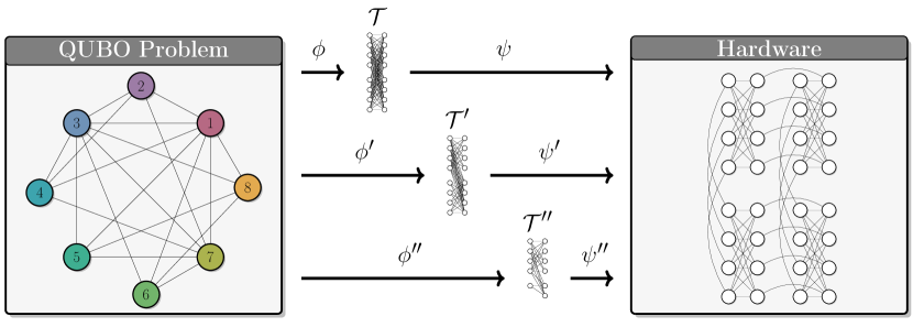
Figure 3: A high-level overview of the virtual hardware framework, including the iterative tuning of the virtual embedding $\phi$, virtual hardware template $\mathcal{T}$, and the physical embedding $\psi$.

Formally, we assume the problem is formulated as a graph $P$ and the hardware layout as a graph $H$. The virtual hardware template $\mathcal{T}$ is a graph embeddable into $H$. This embedding denotes an allocation of qubits in $H$ into virtual qubits in $\mathcal{T}$, encoded with a physical embedding function $\psi:V(\mathcal{T})\to\mathcal{P}(V(P))$. For bookkeeping, we require that each edge in $\mathcal{T}$ represents exactly one edge in $H$ – therefore removing edges in the virtual hardware has a corresponding meaning on the physical hardware footprint. Since we want to define a virtual hardware template that scales with the physical hardware, we define virtual hardware templates in terms of families:

Definition 2 (Chimera-Compatible Virtual Hardware Template Family)

A virtual hardware template family $\mathcal{F}$ is a set of virtual hardware graphs defined with a corresponding family of physical hardware embedding functions $\Psi$, such that for all $L,M,N\in\mathbb{Z}^{+}$, there exists $\psi\in\Psi$ and $\mathcal{T}\in\mathcal{F}$ such that $\psi$ minor embeds $\mathcal{T}$ into $\mathcal{C}_{L,M,N}$.

Finding a virtual embedding function $\phi:V(P)\to\mathcal{P}(V(\mathcal{T}))$ is sufficient for finding the initial embedding $\chi:V(P)\to\mathcal{P}(V(H))$, which can be constructed by letting $\chi(u)=\bigcup_{x\in\phi(u)}\psi(x)$. We compute this virtual embedding function with an embedding subroutine:

Definition 3 (Embedding Subroutine)

An embedding subroutine takes as input a problem graph $P$ and virtual hardware $\mathcal{T}$, and outputs a virtual embedding $\phi:V(P)\to\mathcal{P}(V(\mathcal{T}))$ or the keyword FAIL.

After finding a full minor embedding function, we then apply reduction subroutines to produce tuned embeddings:

Definition 4 (Reduction Subroutine)

A reduction subroutine takes as input a problem $P$, virtual hardware $\mathcal{T}$, and virtual embedding $\phi$, then outputs an updated virtual hardware $\mathcal{T}^{\prime}$ and virtual embedding $\phi^{\prime}$ (potentially identical to $\mathcal{T}$ and $\phi$).

After reduction subroutines are applied, an updated physical embedding function $\psi^{\prime}$ can be recovered from the original $\psi$ and the final virtual hardware $\mathcal{T}^{\prime}$ by using only the physical qubits needed to represent the edges in $\mathcal{T}^{\prime}$. Again, we have a full embedding $\chi^{\prime}$ of the problem into the physical hardware by combining $\phi^{\prime}$ and $\psi^{\prime}$.

3.1 Biclique Virtual Hardware

We now present an implementation of this framework using a biclique virtual hardware, an embedding subroutine based on both Choi’s TRIAD and Klymko et al.’s embedding algorithm, and provide two reduction subroutines for minimizing the total number of qubits used. We start with the virtual hardware:

Definition 5 (Biclique Virtual Hardware Template Family)

A $\mathcal{C}_{L,M,N}$  hardware contains a biclique $K_{LM,LN}$ virtual hardware $\mathcal{T}$ with partite sets $L(\mathcal{T})=\{v_{1},\dots,v_{LM}\}$ and $R(\mathcal{T})=\{h_{1},\dots,h_{LN}\}$; we refer to these as the vertical and horizontal partite sets, respectively. The embedding function defining the minor embedding is given by

$$\psi(v_{i}) =\{(j,\lceil i/L\rceil,1,i\bmod L)~{}|~{}1\leq j\leq M\},\text{ and }$$

$$\psi(h_{i}) =\{(\lceil i/L\rceil,j,2,i\bmod L)~{}|~{}1\leq j\leq N\}.$$

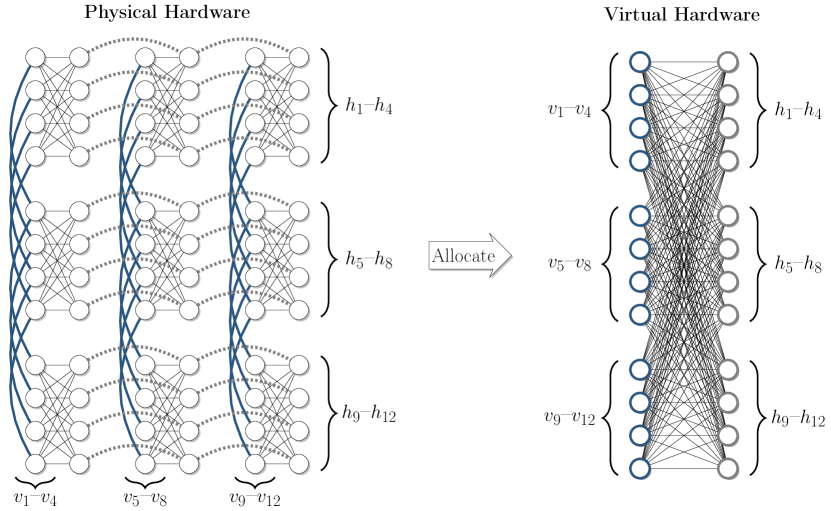
Figure 4: The $K_{12,12}$ biclique virtual hardware for Chimera(4, 3, 3). Thick blue edges show allocations to vertical vertex sets, and dashed gray edges show the horizontal vertex set allocations.

The intuition behind this allocation is a partitioning of the edges in Chimera graphs (c.f. Fig. 4). There are three such edge types – intra-cell, vertical inter-cell, and horizontal inter-cell – and the inter-cell edges provide the highest connectivity increase per minor contraction. Therefore allocating maximal vertical and horizontal paths provides a virtual hardware with relatively large degree per vertex.

The biclique virtual hardware is fairly robust to physical hardware specifications by not requiring a square Chimera grid like previous algorithms, nor depending on the fact that $L=4$ in existing hardware implementations. A biclique virtual hardware can also be allocated from a hardware implementation with hard faults; however, in the naive allocation we find that each missing qubit removes a full vertical or horizontal path. Managing hardware implementations with hard faults is less a concern than in prior work, with more mature hardware yields and the introduction of software post-processing methods for emulating missing qubits (e.g. the Full-Yield Chimera Solver provided in D-Wave SAPI 2.4 sapi ).

3.2 Biclique Embedding and Reduction Subroutines

In this subsection we develop a baseline set of embedding and reduction subroutines utilizing the biclique virtual hardware template. We start by providing an embedding for a complete graph on $\min(LM,LN)$ vertices. At a high level the embedding assignment is straightforward: a single virtual qubit in the vertical partite has edges to every virtual qubit in the horizontal partite, and vice-versa. Therefore, to ensure that every two problem vertices are joined by an edge, we map each problem vertex to a pair of virtual qubits:

Subroutine 1 (Native-Embed)

Given a problem graph $P$ with $V(P)=\{u_{1},\dots,u_{n}\}$ where $n\leq\min(LM,LN)$ and a biclique virtual hardware $\mathcal{T}$ with partites $L(\mathcal{T})=\{v_{1},\dots,v_{LM}\}$ and $R(\mathcal{T})=\{h_{1},\dots,h_{LN}\}$, Native-Embed produces an embedding $\phi$ by mapping $\phi(u_{i})=\{v_{i},h_{i}\}$ for $1\leq i\leq n$.

As defined, Native-Embed redundantly has two edges between every pair of vertex sets $\phi(u_{i})$ and $\phi(u_{j})$, for $i\neq j$; namely, the edges $(v_{i},h_{j})$ and $(v_{j},h_{i})$. Recall that we defined $\psi$ such that each edge in $\mathcal{T}$ represents a unique edge in $H$, so this redundancy in the virtual hardware represents an actual redundancy in the physical embedding. To gauge the wastefulness, we score a virtual hardware and its virtual embedding:

Subroutine 2 (Qubit-Scoring)

Suppose we are given standard input $P$, $\mathcal{T}$, and $\phi$. For each virtual qubit $v_{i}\in L(\mathcal{T})$, let $I_{v_{i}}=\{j~{}|~{}(v_{i},h_{j})\in E(\mathcal{T})\}$ be its index set – the range of neighbors it has on the virtual hardware. Define the score for each left partite vertex as

$$\text{{score}}(v_{i})=1+\left\lfloor\frac{max(I_{v_{i}})}{L}\right\rfloor-\left\lfloor\frac{min(I_{v_{i}})}{L}\right\rfloor.$$

Each $h_{i}$ is assigned an index set and score analogously. Then the qubit score for $\phi$ and $\mathcal{T}$ is

$$\sum_{v_{i}\in L(\mathcal{T})}\text{{score}}(v_{i})+\ \sum_{h_{i}\in R(\mathcal{T})}\text{{score}}(h_{i}).$$

At a high level, Qubit-Scoring computes the number of physical qubits that must be used with the current virtual hardware and virtual embedding. If removing a redundant edge reduces the score, then we have also reduced physical hardware usage. If removing a redundant edge does not affect the score, then we know that this particular edge is not requiring extra hardware usage by itself; however, a sequence of non-score-reducing redundant edge removals could potentially reduce the score. Therefore, it is non-trivial to identify which of the redundant edges should be removed for optimal hardware resource minimization.

Based on this observation, we provide two evaluation methods for computing virtual hardware minimization. First, Qubit-Evaluation computes all possible redundant edge removals and chooses the one with minimum score; this calculation is exponential in the number of redundant edges. A faster evaluation method Fast-Qubit-Evaluation greedily keeps the lexicographically-first edge, providing a minimal (but not necessarily minimum) score in linear time.

Subroutine 3 (Qubit-Evaluation)

Suppose we are given standard input $P$, $\mathcal{T}$, and $\phi$. Let $S$ be the set of problem vertices mapped to at least one virtual qubit on each partite, let $\mathcal{E}$ be the set of all edge sets $E$ on the virtual hardware such that for each $u,v\in S$, there is exactly one edge $(u^{\prime},v^{\prime})\in E$ with $u^{\prime}\in\phi(u)$ and $v^{\prime}\in\phi(v)$. Then Qubit-Evaluation returns $\operatorname*{arg\,min}_{E\in\mathcal{E}}\text{{Qubit-Scoring}(E)}$.

Subroutine 4 (Fast-Qubit-Evaluation)

Suppose we are given standard input $P$, $\mathcal{T}$, and $\phi$. Let $S$ be the set of problem vertices mapped to at least one virtual qubit on each partite. Then Fast-Qubit-Evaluation returns $E=\{(v_{i},h_{j})~{}|~{}i\leq j,~{}v_{i}\in\phi(x),~{}h_{j}\in\phi(y)\text{ for }x,y\in V(P)\text{ and }y\in N(x)\}$.

The last step is to use this reduced edge set to construct a reduced virtual hardware, computed using Qubit-Reduce:

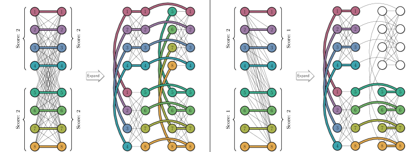
Figure 5: (Left) The Native-Embed embedding with “+”-shaped vertex sets; (Right) The embedding reduced by Qubit-Reduce, with “L”-shaped vertex sets.

Subroutine 5 (Qubit-Reduce)

Given standard input $P$, $\mathcal{T}$, $\phi$ and an evaluation subroutine, Qubit-Reduce computes a set of redundant edges to be removed $E$, and outputs the current virtual embedding $\phi$ and a new virtual hardware $\mathcal{T}^{\prime}$ with vertices $V(\mathcal{T})$ and edges $E(\mathcal{T})-E$.

While fairly simple, Qubit-Reduce has the potential to reduce qubit usage by 50%. This ratio occurs when Native-Embed’s “+”-shaped vertex sets on the physical hardware are reduced to “L”-shaped vertex sets (as described by Boothby et al. boothby2016fast ). Fig. 5 visualizes this reduction.

Up to this point, we have implicitly assumed that the problem graph was complete (i.e. we needed to enforce every edge). However, we can achieve further hardware resource reduction by assuming that the problem is missing edges. Specifically, by shuffling the assignment of vertex sets on the biclique virtual hardware, we can group together those vertices with edges between them, resulting in shorter vertex sets. This computation can be done with a scheme of subroutines, $k$Exchange-Reduce. In local search terminology, we compute a deterministic gradient descent on the $k$-exchange neighborhood without restarts.

Subroutine 6 ($k$Exchange-Reduce)

Given standard input $P,\mathcal{T},\phi$, and neighborhood exchange parameter $k\geq 2$, the subroutine $k$Exchange-Reduce computes a new virtual embedding $\phi^{\prime}$ with the following steps:

1. Let $\phi^{\prime}=\phi$.

2. Starting from $\phi^{\prime}$, compute all $\binom{n}{k}k!$ ways to reassign exactly $k$ problem vertices in each partite, and score each qubit reassignment. (For example, if $\phi(u_{1})=\{v_{1},h_{1}\}$ and $\phi(u_{2})=\{v_{2},h_{2}\}$, then their 2-exchange on the left partite is $\phi(u_{1})=\{v_{2},h_{1}\}$ and $\phi(u_{2})=\{v_{1},h_{2}\}$).

3. Let $\phi^{\prime}$ be the reassignment with the lowest score.

4. Repeat until no $k$-exchange leads to a score reduction, and return $\phi^{\prime}$ and $\mathcal{T}$.

For a fixed $k$, run time for $k$Exchange-Reduce is $\binom{n}{k}k!=O(n^{k})$ per iteration with a maximum of $L^{2}(M+N)$ iterations. With the standard assumptions that $L$ is a constant and $\sqrt{n}=\max(M,N)$, $k$Exchange-Reduce has a run time of $O(n^{k+1/2})$.

3.3 Emulation and Enhancement

Applying the tools introduced in the last subsection, we can emulate Choi’s $K_{LN}$ TRIAD algorithm choi2011minor with Native-Embed and Qubit-Reduce. Klymko et al.’s $K_{LN+1}$ embedding klymko2014adiabatic can be found by tweaking Native-Embed to embed $u_{1},\dots,u_{LN-1}$ as usual, but also setting $\phi(u_{LN})=\{v_{LN}\}$ and $\phi(u_{LN+1})=\{h_{LN}\}$. We note that doing so forces the first $LN-1$ vertex sets to cover both the vertical and horizontal partites in order to be adjacent to the last two vertices, therefore applying Qubit-Reduce has a limited effect and is not recommended for general use.

One advantage of emulating existing algorithms in this framework is for the application of virtual hardware-specific reduction subroutines; namely, Qubit-Reduce and $k$Ex-Reduce. In Section 5.1 we see that the subroutines do in fact produce smaller embeddings without unreasonably increasing run times.

3.4 Summary

In this section we defined a biclique virtual hardware formed naturally from the Chimera graph by exploiting its grid-like structure and high intra-cell connectivity.

We also defined a full baseline stack of embedding and reduction subroutines. As noted in the last subsection, this framework is sufficient for emulating the best existing algorithms for dense problem graphs in hardware layouts without faults. Furthermore, we can apply additional reduction routines to achieve reduced embedding footprints. In total, these results serve as a full proof-of-concept motivating the use of virtual hardware and the development of specialized and modular subroutines. In the next section we take the next step and move beyond existing embedding algorithms by exploiting the bipartite structure in problem graphs to tackle larger, more sparse problems.

4 Utilizing Bipartite Problem Structure

In the last section we emphasized the structural properties of the Chimera hardware graph, deriving the biclique virtual hardware and its subroutines. In this section we utilize bipartite structure from the problem graph. Specifically, we use the notion of odd cycle transversals to decompose problem graphs and extract a maximal bipartite induced subgraph. We start by defining the odd cycle transversal and its limitations in the Chimera graph, then describe an initial embedding subroutine OCT-Embed, and finally propose a faster heuristic, Fast-OCT-Embed.

4.1 Odd Cycle Transversal

One metric for gauging the “bipartite-ness” of a graph $G$ is the smallest set of vertices preventing $G$ from being bipartite, a minimum odd cycle transversal:

Definition 6 (Odd Cycle Transversal (OCT))

The odd cycle transversal of a graph $G$ is a set of vertices $S$ such that $G\setminus S$ is a bipartite graph. We denote the size of a minimum OCT set as the OCT number, $OCT(G)$, and the problem of computing $OCT(G)$ as MinOCT.

Unfortunately, MinOCT is NP-hard lewis1980node and does not have a constant factor approximation algorithm unless P = NP lund1993approximation . However, the problem is fixed-parameter tractable (FPT) when parameterized by the natural parameter (solution size). In other words, graphs with small OCT numbers will also have quickly-computable OCT numbers, regardless of total graph size. Given that the biclique virtual hardware is most efficiently utilized when embedding problem graphs with small OCT numbers, we expect embeddable problem graphs will have an efficiently computable OCT decomposition. As a baseline we use Reed et al.’s $O(3^{k}kmn)$ algorithm for computing solutions of size $k$, which is known to have several simplifications and optimizations lokshtanov2009simpler ; huffner2005algorithm . Other algorithms for specialized instances also exist agarwal2005approximation ; lokshtanov2012subexponential .

We note that MinOCT and the problem of computing the size of the maximum bipartite induced subgraph (denoted by MaxBipartite) are complements, in the sense that an exact solution to one problem also provides a solution to the other. However, an approximation for one problem is not an approximation for the other, so some care must be taken when choosing which problem to approximate.

4.2 OCT and the Chimera Graph

In prior work, Klymko et al. showed that the Chimera graph has treewidth bounded by $O(LN)$, assuming $N\leq M$ klymko2014adiabatic . In this section we show that the maximum $OCT(G)$ over all Chimera-embeddable graphs $G$ is bounded by all three Chimera parameters. First, we note that treewidth and OCT describe different graph structure:

Proposition 1

The treewidth of a graph is independent of its OCT number.

Proof

Consider two families of graphs:

1. The class of grid graphs. These graphs are known to have treewidth proportional to the smallest grid dimension diestel2005graph , but have an OCT number of 0 since they are bipartite.

2. The class of trees with their leaves replaced with triangles. These graphs have treewidth at most three (a tree decomposition exists where each bag contains at most a triangle and its neighbor in the tree), but unbounded OCT number since each (disjoint) triangle contains at least one OCT vertex.

We have shown that one property cannot bound the other, therefore they are independent. ∎∎

With this independence established, we proceed to show upper and lower bounds on the maximum OCT number of a Chimera-embeddable graph.

Lemma 1

$OCT(G)\leq\min(|L(B)|,|R(B)|)$ for all minors $G$ of a bipartite graph $B$ with vertex partite sets $L(B)$ and $R(B)$.

Proof

Let $\phi$ be a minor embedding of $G$ into $B$, and without loss of generality, let $L(B)$ be the smaller of the two partite sets. Let $S=\{x~{}|~{}x\in V(G)\text{ and }u\in\phi(x)\text{ for }u\in L(B)\}$, then we know that $|S|\leq|L(B)|$. $V(G)-S$ is necessarily bipartite since $\phi(x)$ is composed of vertices from $R(B)$ for $x\in V(G)-S$, therefore $OCT(G)\leq|S|\leq|L(B)|$. ∎∎

Corollary 1

$OCT(G)\leq LMN$ for all Chimera-embeddable graphs $G$.

Lemma 2

There exists a Chimera-embeddable graph $G$ such that $OCT(G)\geq(L-1)MN$.

Proof

We construct $G$ by contracting $L-1$ vertex-disjoint edges in each cell of a Chimera graph. Each cell is now a $K_{L+1}$ clique and $L-1$ of these vertices must be included in an OCT set, therefore $OCT(G)\geq(L-1)MN$. ∎∎

While the treewidth of Chimera graphs only grows in two dimensions ($L$ and $\min(M,N)$), Lemma 2 shows that the minimum odd cycle transversal will increase if $L$, $M$, or $N$ is increased. Therefore we recommend using a minimal odd cycle transversal as a proxy for estimating how much hardware a problem graph’s embedding will require. A minimal OCT set is fast to compute and reflects more of the actual hardware usage than treewidth.

In addition to gauging how much hardware a problem’s embedding will require, we can also use the minimum odd cycle transversal to recognize when certain problems are not embeddable. The Klymko et al. klymko2014adiabatic result shows that problems with treewidth larger than $(L+1)N$ cannot be embedded, but this bound does not apply to classes of small treewidth, such as series-parallel graphs eppstein1992parallel . However, the OCT rejection criterion provides a characterization of unembeddable graphs in terms of odd cycles, therefore it encompasses a different class of graphs (including series-parallel graphs, which can have an unbounded number of odd cycles).

4.3 Computing OCT and OCT-Embed

As mentioned previously, the fastest-known algorithm for computing the OCT number is exponential in the solution size, so we want to prune graphs if possible. One method of doing that is by removing tree-like structure:

Proposition 2

To compute MinOCT on a graph $G$, it is sufficient to compute MinOCT on the maximal 2-edge-connected subgraphs of $G$.

Proof

We induct on the number of 2-edge-connected maximal subgraphs. If there is no such subgraph, then every edge is a bridge and the graph is a tree, therefore the claim is true.

Suppose instead that there are $k$ such subgraphs in $G$ and the claim is true for all graphs with $k-1$ such subgraphs. We can decompose the graph into maximal 2-edge-connected subgraphs by computing a chain decomposition schmidt2013simple on $G$ to identify its bridges. Removing these bridges produces each maximal 2-edge-connected subgraph as a connected component. Further, contracting these subgraphs creates a tree with the contracted subgraphs as vertices and the bridges as the edges. Pick a subgraph $S$ that is a leaf on this tree, and let $(v_{1},v_{2})$ be the bridge separating $S$ from $G\setminus S$. By the induction hypothesis, we can compute $OCT(G\setminus S)$ and $OCT(S)$ on their maximal 2-edge-connected subgraphs, therefore all that remains is to show that these two partial solutions are compatible.

Suppose that the partial solutions are expressed as a coloring: vertices in the left partite set are colored $L$, the right partite set $R$, and neither partite set (e.g. in the OCT set) as $N$. If at least one of $v_{1},v_{2}$ is colored $N$, or if one is colored $L$ and the other $R$, then these partial solutions are compatible as-is. Suppose to the contrary that both are colored with the same partite set color. Then in $S$ we recolor $L\to R$ and $R\to L$. This recoloring does not change $OCT(S)$, and the partial solutions are now compatible. ∎∎

This preprocessing step is fast, costing only an additive $O(m)$ run time when using Schmidt’s chain decomposition algorithm schmidt2013simple . This approach also provides an opportunity for parallelization if the graph has many 2-edge-connected maximal subgraphs. While this technique applies to any graph, we can take advantage of the 2-edge-connectivity in the class of series-parallel graphs by exploiting nested ear decompositions:

Proposition 3

$OCT(G)$ can be computed in linear time for a series-parallel graph $G$.

Proof

The proof of Proposition 3 can be found in Appendix A. ∎∎

We conclude this subsection by defining an embedding subroutine that uses an OCT-decomposition to embed into the biclique virtual hardware. At a high level, OCT-Embed first computes a minimum OCT set, embeds the OCT vertices as if they were a complete graph, and then embeds the bipartite induced subgraph directly into the biclique virtual hardware (Fig. 6.

Subroutine 7 (OCT-Embed)

Let $P$ be a problem graph with $V(P)=S\cup L\cup R$, where $S=\{u_{1},\dots,u_{i}\}$ is a minimum OCT set, and $L=\{u_{i+1},\dots,u_{j}\}$ and $R=\{u_{j+1},\dots,u_{n}\}$ are a maximum bipartite induced subgraph. Let $\mathcal{T}$ be a biclique virtual hardware with partites $L(\mathcal{T})=\{v_{1},\dots,v_{LM}\}$ and $R(\mathcal{T})=\{h_{1},\dots,h_{LN}\}$. If $j\leq LM$ and $n-i\leq LN$, then OCT-Embed produces an embedding $\phi$ by mapping:

$$\phi(u_{x}) =\left\{\begin{array}[]{ll}\{v_{x},h_{x}\}\text{ if }u_{x}\in S\\ \{v_{x}\}\text{ if }u_{x}\in L\\ \{h_{x-i}\}\text{ if }u_{x}\in R\end{array}\right.$$

otherwise it outputs FAIL.

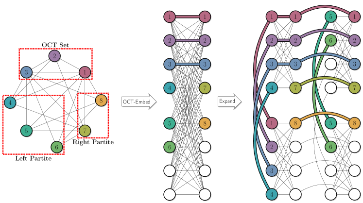
Figure 6: Embedding an 8-vertex problem into $\mathcal{C}_{4,2,2}$ using the OCT-Embed subroutine. For figure readability, vertex $u_{i}$ is labeled with $i$.

4.4 Approximating OCT and Fast-OCT-Embed

A downside to OCT-Embed is its exponential run time, restricting the subroutine’s real-world applicability. However, an exact solution to MinOCT is not always required for a full embedding – any odd cycle transversal decomposition will work as long as it fits into the biclique virtual hardware. We utilize this fact to develop an approximation algorithm for MaxBipartite, and use this approximation algorithm for two purposes: (1) as an initial solution for the iterative compression in our algorithm for OCT-Embed, and (2) as a standalone embedding subroutine Fast-OCT-Embed.

We approximate MaxBipartite instead of MinOCT for two reasons. First, the Reed et al. algorithm reed2004finding we use to compute the exact OCT number uses a technique called iterative compression, where a solution of size $k+1$ is compressed to size $k$ over several subgraph iterations. We can reduce the number of these iterations by providing the algorithm with a large initial subgraph with at most $k$ OCT vertices, therefore we have motivation for estimating a maximal bipartite subgraph. Second, if we approximate MaxBipartite, then our worst approximations (in terms of magnitude) are when the graph has a large bipartite graph. However, this implies a small OCT set, therefore the exact algorithm will have an exponentially faster run time. Therefore approximating MaxBipartite makes more sense in this context.

Our approximation algorithm is outlined in Algorithm 1. Partially motivated by the success of using a greedy algorithm to compute exact solutions on series-parallel graphs, we found that a minimum-degree–greedy algorithm also performed well in practice on general graphs (c.f. Section 5.1). In total, the algorithm has a run time of $O(m)$ using a modification of Bataglj and Zavers̆nik’s algorithm for computing $k$-core decompositions batagelj2003algorithm .

Algorithm 1 Greedy Maximal Bipartite Induced Subgraph

1:function GreedyBipartite($G$)

2:     $L\leftarrow\textsf{GreedyIndSet}(G)$

3:     $R\leftarrow\textsf{GreedyIndSet}(G\setminus L)$

4:     return $L\cup R$

5:end function

6:

7:function GreedyIndSet($G$)

8:     $S\leftarrow\emptyset$

9:     while $G$ not empty do

10:         $v\leftarrow\operatorname*{arg\,min}_{u\in V(G)}d(u)$ $\triangleright$ Pick any min degree vertex

11:         $S\leftarrow S\cup\{v\}$

12:         $G\leftarrow G\setminus(\{v\}\cup\textsc{N}(v))$

13:     end while

14:     return $S$

15:end function

We begin the approximation factor analysis by noting that an approximation algorithm for minimum independent set translates to MaxBipartite:

Lemma 3

GreedyBipartite implemented with an $\alpha$-approximation GreedyIndSet algorithm is an $\alpha$-approximation algorithm.

Proof

Let $S$ be a fixed set of vertices such that $G[S]$ is the larger partite of a maximum bipartite induced subgraph. We want to show that for every vertex GreedyBipartite adds to its solution $S^{\prime}$, at most $\alpha$ vertices from $S$ are not chosen. Let $L$ and $R$ be the first and second independent sets constructed by GreedyIndSet, respectively. First, the set $L$ is chosen without (immediately) disqualifying any vertex in $G\setminus L$ from being in $R$, so no vertices are disqualified from $S^{\prime}$ in this step. When constructing $R$, at most $\alpha$ vertices from $S$ are disqualified for every vertex added to $R$, by definition of the approximation factor. Therefore $R$ itself is an $\alpha$-approximation for the partite and a $2\alpha$-approximation for MaxBipartite. If $|L|\geq|R|$ then we have shown at least an $\alpha$-approximation. To show the approximation factor still holds when $|L|<|R|$, we want to show that $L$ is a $\alpha$-approximation for MaxIndSet in $G\setminus R$. But the previous argument still holds, since at most $\alpha$ vertices from $S$ are disqualified from $S^{\prime}$ for every vertex chosen from $G\setminus R$. Therefore in both cases we have a $alpha$-approximation for the larger partite of a maximum induced bipartite subgraph, therefore we have an $\alpha$-approximation for MaxBipartite. ∎∎

Corollary 2

GreedyBipartite is a $\frac{\Delta+2}{3}$-approximation and a $\frac{2\bar{d}+3}{5}$-approximation for graphs with maximum degree $\Delta$ and average degree $\bar{d}$.

Proof

Halldórsson and Radhakrishnan halldorsson1994greed show that GreedyIndSet is a $\frac{\Delta+2}{3}$-approximation and a $\frac{2\bar{d}+3}{5}$-approximation for maximum independent set. By Lemma 3, the same approximation factors hold for GreedyBipartite. ∎∎

Corollary 3

GreedyBipartite is a $d$-approximation for $d$-degenerate graphs.

Proof

We first want to show that GreedyIndSet is a $d$-approximation, this proof mirrors that of Lemma 3. Fix a maximum independent set $S$. In each step of GreedyIndSet, a vertex added to the solution disqualifies at most $d$ vertices from $S$. Therefore GreedyIndSet is a $d$-approximation for a maximum independent set, and applying Lemma 3 shows that GreedyBipartite is a $d$-approximation for MaxBipartite. ∎∎

Up to this point we have not assumed anything about the OCT set when computing an approximation factor. However, as graphs get more dense the OCT set must also grow. We can show this by using degeneracy as a metric for density:

Definition 7 (Graph Degeneracy)

The degeneracy of a graph $G$ is the smallest $k$ such that every subgraph of $G$ has a vertex of degree at most $k$.

Lemma 4

GreedyBipartite is a $(n-d)$-approximation for a $d$-degenerate graph when $d\geq\frac{n}{2}$.

Proof

When $d\leq\frac{n}{2}$, the desired graph can always be found as a subset of $K_{n/2,n/2}$. However, for larger values of $d$, vertices must be moved from the bipartite graph into the OCT set, specifically two vertices per additional unit of degeneracy. This fact means that a $d$-degenerate graph can have at most a bipartite subgraph on $2(n-d)$ vertices. Solving for the approximation factor: $\alpha\cdot 2(n-d)=\frac{2n}{d}$, so $\alpha=\frac{2n}{2d(n-d)}=\frac{n}{n-d}\cdot\frac{1}{d}\geq\frac{n}{n-d}\cdot\frac{1}{n}=\frac{1}{n-d}$. ∎∎

Proposition 4

Fast-OCT-Embed is a $\min(d,n-d)$-approximation for $d$-degenerate graphs.

Proof

This result follows directly from Lemmas 3 and 4. ∎∎

In other words, the degeneracy-based approximation factor is best on very sparse and very dense graphs. Swapping the approximation algorithm into our embedding subroutine, we now define Fast-OCT-Embed:

Subroutine 8 (Fast-OCT-Embed)

Let $P$ be a problem graph with $V(P)=S\cup L\cup R$, where $S=\{u_{1},\dots,u_{i}\}$ is an OCT set, and $L=\{u_{i+1},\dots,u_{j}\}$ and $R=\{u_{j+1},\dots,u_{n}\}$ are a maximum bipartite induced subgraph. Let $\mathcal{T}$ be a biclique virtual hardware with partites $L(\mathcal{T})=\{v_{1},\dots,v_{LM}\}$ and $R(\mathcal{T})=\{h_{1},\dots,h_{LN}\}$. If $j\leq LM$ and $n-i\leq LN$, then OCT-Embed produces an embedding $\phi$ by mapping:

$$\phi(u_{x}) =\left\{\begin{array}[]{ll}\{v_{x},h_{x}\}\text{ if }u_{x}\in S\\ \{v_{x}\}\text{ if }u_{x}\in L\\ \{h_{x-i}\}\text{ if }u_{x}\in R\end{array}\right.$$

otherwise it outputs FAIL.

4.5 Summary

In summary, the odd cycle transversal provides a structured method for decomposing problems and embedding them smartly into the Chimera hardware. We showed that OCT is a more flexible property than treewidth in Chimera, increasing flexibility to new generations of hardware, and also showed how to use OCT to embed into a biclique virtual hardware. In the next section we evaluate these new embedding subroutines against previously studied embedding algorithms.

5 Experimental Results

In this section we experimentally evaluate virtual hardware against the existing benchmark algorithms. First, we compare the approximation Fast-OCT-Embed against the exact OCT-Embed, using no reduction routines. We then compare the Reduced Fast-OCT-Embed against Cai et al.’s Dijkstra-based heuristic (denoted here as CMR (Dijkstra)). Finally we conclude with a comparison again Choi’s TRIAD algorithm for embedding complete graphs. Against both benchmarks we find that Reduced Fast-OCT-Embed finds embeddings for larger graphs, using less qubits, with fast run times (less than a second).

To minimize bias in the cross-algorithm comparisons, all algorithms and subroutines (e.g. breadth-first search, Dijkstra’s algorithm, etc.) were implemented manually in C++ and are available at https://github.com/TheoryInPractice/aqc-virtual-embedding.

OCT-Embed is implemented using Lokshtanov et al.’s simplification of Reed et al.’s iterative compression algorithm lokshtanov2009simpler ; reed2004finding . Fast-OCT-Embed is computed using the smallest OCT number found with $10,000$ runs of GreedyBipartite; run times reported include the total run time to collect this distribution. Reduced Fast-OCT-Embed additionally applies Qubit-Reduce and 2Ex-Reduce using Fast-Qubit-Scoring.

We implemented the CMR (Dijkstra) algorithm from the Dijkstra-based pseudocode provided on page 7 of cai2014practical . Since this heuristic does not necessarily produce an embedding if it exists, we run the heuristic repeatedly until an embedding is found or the time cutoff is reached; this provides the expected time to find an embedding. TRIAD is implemented with Choi’s deterministic algorithm, and Reduced TRIAD uses the biclique virtual hardware with Qubit-Reduce and 2Ex-Reduce using Fast-Qubit-Scoring.

To provide a broad spectrum of comparisons, we generated problem graphs using four random graph generators at three density levels (Table 1). While previous algorithms such as CMR have been tested on problem graphs with constant vertex degree (e.g. grid and 3-regular graphs), this assumption is unrealistic for real-world QUBOs. Intuitively, the complexity of the problem should scale with the number of variables included. As an example, we note that Beasley’s QUBOs beasley1990or have average vertex degree of approximately $\frac{n}{20}$ for $n$ vertex problems.

We define the random graph models as follows. Noisy bipartite graphs were generated by splitting the vertices evenly (up to parity) into two partite sets, including a bipartite edge at probability $p$, and including a non-bipartite edge at probability $\frac{p}{5}$. The GNP graphs (also known as Erdős-Rényi erdos1960evolution ) are generated by flipping a coin for each possible edge and including it with probability $p$. The regular graph generator samples from the space of graphs where each vertex has degree exactly $k$. Barabási-Albert graphs albert2002statistical are generated by iteratively attaching $n-k$ vertices to a subgraph of $k$ vertices using preferential attachment; we generate the initial subgraph using GNP with $p=0.25$. All graphs are generated using the NetworkX implementations hagberg2008exploring , excepting Barabási-Albert, which required a modification to generate the initial subgraph as specified above.

Graph Family	Low Density	Medium Density	High Density
Noisy Bipartite	$p=0.25$	$p=0.50$	$p=0.75$
GNP	$p=0.25$	$p=0.50$	$p=0.75$
Regular	$k=0.25n$	$k=0.50n$	$k=0.75n$
Barabasi-Albert	$k=0.25n$	$k=0.50n$	$k=0.75n$

Table 1: Definition of density levels for the random input graph generators.

All experiments were run on a workstation running Fedora 24, and were each allocated a core on an Intel X5675 processor and 1GB of RAM. Run times were limited to 60 minutes using the timeout -k 10s 60m command, and no algorithm used more than its allocated memory. The C++ code was compiled with g++ 5.3.1 at the -O2 optimization level, and controlled with wrapper scripts run with Python 2.7.11. All experiments were seeded using the number of seeds specified in each experiment below. The data points plotted are the median over all problem graph instances and seeded algorithm runs.

5.1 Experimental Results

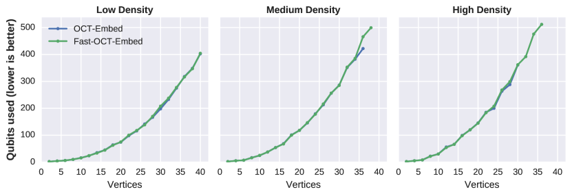
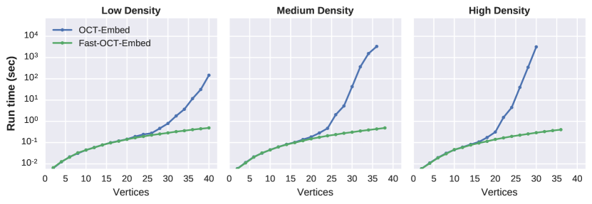
Figure 7: Embedding GNP graphs into Chimera(4, 8, 8); data points are the median over 25 random graphs and 10 random algorithm seeds. Experimentally, we observe that the approximation algorithm performs notably better than its approximation factor guarantees, while additionally achieving highly practical run times.

Comparing OCT-Embed and Fast-OCT-Embed on 25 graph instances per $n$ value and 10 seeded algorithm runs, we find that Fast-OCT-Embed practically matches the solution quality of the exact algorithm, while running in under a second. We report a representative sample in Fig. 7.

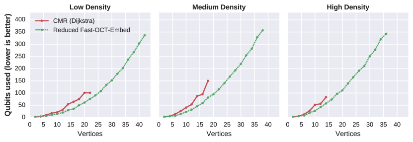
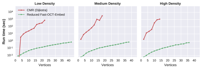
Figure 8: Embedding GNP graphs into Chimera(4, 8, 8); data points are the median over 10 random graphs and 10 random algorithm seeds. Reduced Fast-OCT-Embed consistently outperforms CMR in both qubits used and run time.

To maintain a reasonable run time while maintaining 10 graph instances per $n$, we reduced the comparison with CMR to 10 seeded algorithm runs; this reduction did not impact the results since both CMR (Dijkstra) and Reduced Fast-OCT-Embed restart automatically as needed. We found that CMR (Dijkstra) could not find smaller embeddings than Fast-OCT-Embed, in addition to having significantly longer run times. While CMR may be competitive on very sparse graphs (e.g. grid graphs), we found that it was not competitive when the problem graph had a linear density. Fig. 8 contains a representative sample using GNP.

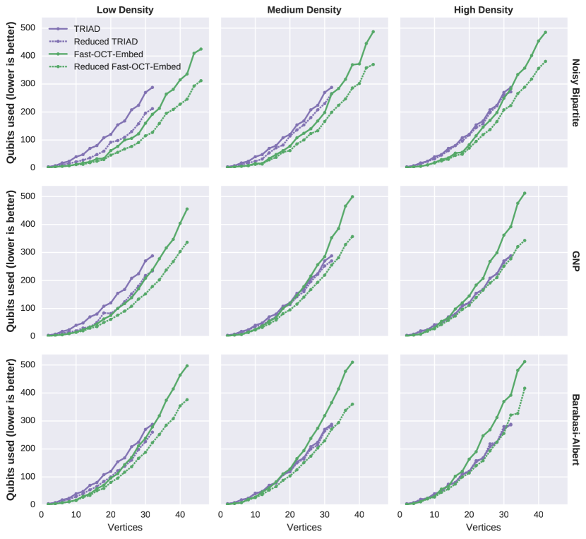
Figure 9: Qubits used when embedding into Chimera(4, 8, 8); data points are the median over 25 random graphs and 10 random algorithm seeds. OCT-based algorithms consistently embed larger problem than possible with TRIAD.

Our final comparison is against Choi’s TRIAD embedding algorithm, the state-of-the-art for embedding highly dense problem graphs in hardware without hard faults. We do not report run times, given that Choi’s algorithm is a deterministic assignment and the OCT-based algorithm’s run times are reported in previous plots. For this experiment we again used 25 problem seeds and 10 algorithm seeds. Fig. 9 contains a representative sample. Again we find that Reduced Fast-OCT-Embed embeds larger graphs while using less qubits. We also note that Reduced TRIAD was effective compared to stock TRIAD for all low density graphs and some medium density graphs, while only adding less than a second to the run time. Moreover, in several scenarios Reduced TRIAD performed better than vanilla OCT-Embed, given the “L”- vs. “+”-shaped embeddings. However, the flexibility provided with “+”-shaped embeddings made the reduction subroutines much more effective, ultimately producing a better full algorithm. As a best practice, then, we recommend that embedding algorithm designers apply these standard reduction subroutines before evaluating an embedding algorithm’s effectiveness.

6 Conclusion

We have developed a virtual-hardware–based framework for constructing and deploying optimized techniques for distinct parts of the minor embedding process. By introducing a biclique virtual hardware, we provide a cleaner interface for embedding into the Chimera hardware layout and enable modular subroutines for qubit reduction. Exploiting the bipartite structure in problem graphs with odd cycle transversals, we are able to embed problems from from a diverse set of generators and densities. Combining these two methods leads to an embedding algorithm Reduced Fast-OCT-Embed that embeds larger problems, while using less qubits, for reasonably dense problem graphs. Moreover, without any parallelization or system-specific tuning, Reduced Fast-OCT-Embed terminates in the order of seconds. This algorithm sets a baseline for embedding dense problem graphs that should be extended and tuned for the user’s application.

Future extensions of this work could include tuned implementation of the reduction methods, which are particularly promising for GPU parallelization. Additionally, as the problem graph becomes highly dense, we see that OCT-Embed (by definition) converges to TRIAD. A more intricate embedding algorithm might not assume the OCT vertices were a clique, allowing even more flexible embeddings. Finally, adapting more intricate embedding algorithms (such as CMR) could provide even better improvements, but would require significant development in the choice of relevant virtual hardware(s).

7 Acknowledgements

The authors would like to thank Steve Reinhardt and the anonymous two reviewers for feedback. This work is supported in part by the Gordon & Betty Moore Foundation’s Data-Driven Discovery Initiative through Grant GBMF4560 to Blair D. Sullivan, a National Defense Science & Engineering Graduate Fellowship and a fellowship by the National Space Grant College and Fellowship Program and the NC Space Grant Consortium to Timothy D. Goodrich.

Appendix A Computing OCT in Series-Parallel Graphs

In this appendix we prove the following result:

Proposition 5

$OCT(G)$ can be computed in linear time for a series-parallel graph $G$.

The proof is based on the equivalence between series-parallel graphs and graphs with nested ear decompositions. Using this decomposition, we show that a greedy algorithm constructs a minimum OCT set. We start by defining series-parallel graphs and nested ear decompositions:

Definition 8 (Eppstein eppstein1992parallel )

A graph $G$ is two-terminal series-parallel with terminals $s$ and $t$ if it can be produced by a sequence of the following operations:

1. Base case: Create new graph, consisting of a single edge directed from $s$ to $t$.

2. Parallel composition: Given two-terminal series-parallel graphs $X$ and $Y$ with terminals $s_{X}$, $t_{X}$, $s_{Y}$, and $t_{Y}$, form a new graph $G=P(X,Y)$ by identifying $s=s_{X}=s_{Y}$ and $t=t_{X}=t_{Y}$.

3. Series composition: Given two-terminal series-parallel graphs $X$ and $Y$, with terminals $s_{X}$, $t_{X}$, $s_{Y}$, form a new graph $G=S(X,Y)$ by identifying $s=s_{X}$, $t_{X}=s_{Y}$, and $t=t_{Y}$.

Definition 9 (Ear Decomposition (Eppstein eppstein1992parallel ))

An ear decomposition of an undirected graph $G$ is defined to be a partition of the edges of $G$ into a sequence of ears $(E_{1},E_{2},\dots,E_{k})$. Each ear is a path in the graph with the following properties:

1. If two vertices in the path are the same, they must be two endpoints of the path.

2. The two endpoints of each ear $E_{i}$, $i>1$, appear in previous ears $E_{j}$ and $E_{j}^{\prime}$, with $j<i$ and $j^{\prime}<i$.

3. No interior point of $E_{i}$ is in $E_{j}$ for any $j<i$.

Definition 10 (Nest Intervals (Eppstein eppstein1992parallel ))

Given an ear decomposition $(E_{1},E_{2},\dots,E_{k})$, we say that $E_{i}$ is nested in $E_{j}$ if both endpoints of $E_{i}$ are contained in $E_{j}$. The nest interval of $E_{i}$ in $E_{j}$ is the path in $E_{j}$ between the two endpoints of $E_{i}$.

Definition 11 (Nested Ear Decomposition (Eppstein eppstein1992parallel ))

An ear decomposition is nested if the following hold:

1. For each $i>1$ there is some $j<i$ such that $E_{i}$ is nested in $E_{j}$.

2. If two ears $E_{i}$ and $E_{i^{\prime}}$ are both nested in the same ear $E_{j}$, then either the nest interval of $E_{i}$ contains that of $E_{i^{\prime}}$ or vice versa.

Eppstein’s result shows that these two graph classes are equivalent:

Theorem A.1 (Eppstein eppstein1992parallel )

Any undirected two-terminal series-parallel graph has a nested ear decomposition starting with a path between the terminals, and any undirected graph with a nested ear decomposition is two-terminal series-parallel with its terminals being the endpoints of the first ear.

Furthermore, Eppstein shows that these decompositions can be computed in $O(\log^{2}(n))$ time on a parallel computer, therefore computing the decomposition itself will not bottleneck an OCT-computing algorithm. We now show that given a nested ear decomposition, we can greedily compute a minimum OCT set. First, we define the parity of ears.

Definition 12 (Ear Parity)

We say that an ear $E_{i}$ is odd if the number of vertices in $E_{i}$ and its nest interval sum to an odd number. We define an even ear analogously.

Next, we want to show that we can compute the minimum OCT set on a single nest interval correctly.

Lemma 5

Given an ear decomposition $(E_{1},\dots,E_{k})$, let $E=(E_{i},\dots,E_{j})$ be an ordered, maximal list of ears contained in a single nest interval. Then the minimum number of OCT vertices contained in these ears is number of maximal in-order sublists of $E$ composed only of odd ears.

Proof

We proceed by induction on the number of sublists. Suppose that there are zero maximal sublists of odd ears, therefore every ear is even. Then every path from the left-most vertex on the nest interval to the right-most vertex on the nest interval will have the same parity, and we are able to two-color these cycles and the minimum OCT number is zero. Suppose instead that there is one maximal sublist of odd ears, therefore all ears are odd. Removing an endpoint from the inner-most odd cycle renders the remaining edges of this smallest nest interval into bridges that cannot be part of a cycle. This removal also breaks all odd cycles in the maximal nest interval, because any cycle on the remaining ears must use the vertices from two odd cycles of length $2x+1$ and $2y+1$, minus the length of the smallest nest interval twice, leaving an odd number of vertices in the cycle. Again we can two-color these and we are done.

Suppose we have an interval with $k$ maximal sublists. If there are any even ears on the outside then we can remove them using the first base case. We now find the inner-most odd ear that is outside of every remaining even ear. Removing an endpoint from this ear renders the outer odd ears bipartite by the second base case. Applying the inductive hypothesis to the earlier ears finds $k-1$ OCT vertices, therefore we have found a total of $k$ OCT vertices. ∎∎

Corollary 4

We can compute the minimum OCT number of the ears contained in a single maximal nest interval in linear time.

Proof

In the above proof we visited each ear once. ∎∎

Proposition 6

$OCT(G)$ can be computed in linear time for a series-parallel graph $G$.

Proof

We proceed by induction on the number of maximal nest intervals. If there are no nest intervals then we have a single ear and are done, the graph is (by definition) bipartite. Otherwise there is some nest interval. Applying Lemma 5, we can compute a minimum OCT set. Since every nest interval is disjoint, by definition, we can apply the inductive hypothesis to compute the minimum OCT set of the other intervals, visiting each interval exactly once. The number of intervals is bounded by the number of vertices, therefore we compute a minimum OCT set in linear time. ∎∎

References

- (1) Agarwal, A., Charikar, M., Makarychev, K., Makarychev, Y.: approximation algorithms for min UnCut, min 2CNF deletion, and directed cut problems. In: Proceedings of the thirty-seventh annual ACM symposium on Theory of computing, pp. 573–581. ACM (2005)
- (2) Albert, R., Barabási, A.L.: Statistical mechanics of complex networks. Reviews of modern physics 74(1), 47 (2002)
- (3) Batagelj, V., Zaversnik, M.: An algorithm for cores decomposition of networks. arXiv preprint cs/0310049 (2003)
- (4) Beasley, J.E.: OR-Library: distributing test problems by electronic mail. Journal of the operational research society pp. 1069–1072 (1990)
- (5) Boothby, T., King, A.D., Roy, A.: Fast clique minor generation in Chimera qubit connectivity graphs. Quantum Information Processing 15(1), 495–508 (2016)
- (6) Boros, E., Hammer, P.L.: Pseudo-boolean optimization. Discrete applied mathematics 123(1), 155–225 (2002)
- (7) Britt, K.A., Humble, T.S.: High-performance computing with quantum processing units. arXiv preprint arXiv:1511.04386 (2015)
- (8) Cai, J., Macready, W.G., Roy, A.: A practical heuristic for finding graph minors. arXiv preprint arXiv:1406.2741 (2014)
- (9) Choi, V.: Minor-embedding in adiabatic quantum computation: I. The parameter setting problem. Quantum Information Processing 7(5), 193–209 (2008)
- (10) Choi, V.: Minor-embedding in adiabatic quantum computation: II. Minor-universal graph design. Quantum Information Processing 10(3), 343–353 (2011)
- (11) D-Wave Systems Inc.: SAPI 2.4 (2016)
- (12) Denchev, V.S., Boixo, S., Isakov, S.V., Ding, N., Babbush, R., Smelyanskiy, V., Martinis, J., Neven, H.: What is the computational value of finite-range tunneling? Physical Review X 6(3), 031,015 (2016)
- (13) Diestel, R.: Graph theory. Graduate Texts in Mathematics 173 (2005)
- (14) Eppstein, D.: Parallel recognition of series-parallel graphs. Information and Computation 98(1), 41–55 (1992)
- (15) Erdos, P., Rényi, A.: On the evolution of random graphs. Publ. Math. Inst. Hung. Acad. Sci 5(1), 17–60 (1960)
- (16) Farhi, E., Goldstone, J., Gutmann, S., Sipser, M.: Quantum computation by adiabatic evolution. arXiv preprint quant-ph/0001106 (2000)
- (17) Hagberg, A.A., Schult, D.A., Swart, P.J.: Exploring network structure, dynamics, and function using NetworkX. In: Proceedings of the 7th Python in Science Conference (SciPy2008), pp. 11–15. Pasadena, CA USA (2008)
- (18) Halldórsson, M., Radhakrishnan, J.: Greed is good: Approximating independent sets in sparse and bounded-degree graphs. In: Proceedings of the twenty-sixth annual ACM symposium on Theory of computing, pp. 439–448. ACM (1994)
- (19) Hamilton, K.E., Humble, T.S.: Identifying the minor set cover of dense connected bipartite graphs via random matching edge sets. arXiv preprint arXiv:1612.07366 (2016)
- (20) Hüffner, F.: Algorithm engineering for optimal graph bipartization. In: International Workshop on Experimental and Efficient Algorithms, pp. 240–252. Springer (2005)
- (21) Humble, T.S., McCaskey, A.J., Bennink, R.S., Billings, J.J., D’Azevedo, E., Sullivan, B.D., Klymko, C.F., Seddiqi, H.: An integrated programming and development environment for adiabatic quantum optimization. Computational Science & Discovery 7(1), 015,006 (2014)
- (22) Humble, T.S., McCaskey, A.J., Schrock, J., Seddiqi, H., Britt, K.A., Imam, N.: Performance models for split-execution computing systems. In: Parallel and Distributed Processing Symposium Workshops, 2016 IEEE International, pp. 545–554. IEEE (2016)
- (23) Kadowaki, T., Nishimori, H.: Quantum annealing in the transverse ising model. Physical Review E 58(5), 5355 (1998)
- (24) Kassal, I., Whitfield, J.D., Perdomo-Ortiz, A., Yung, M.H., Aspuru-Guzik, A.: Simulating chemistry using quantum computers. Annual review of physical chemistry 62, 185–207 (2011)
- (25) King, J., Yarkoni, S., Raymond, J., Ozfidan, I., King, A.D., Nevisi, M.M., Hilton, J.P., McGeoch, C.C.: Quantum annealing amid local ruggedness and global frustration. arXiv preprint arXiv:1701.04579 (2017)
- (26) Klymko, C., Sullivan, B.D., Humble, T.S.: Adiabatic quantum programming: minor embedding with hard faults. Quantum information processing 13(3), 709–729 (2014)
- (27) Leighton, F.T.: Introduction to parallel algorithms and architectures: Arrays· trees· hypercubes. Elsevier (2014)
- (28) Lewis, J.M., Yannakakis, M.: The node-deletion problem for hereditary properties is NP-complete. Journal of Computer and System Sciences 20(2), 219–230 (1980)
- (29) Lokshtanov, D., Saurabh, S., Sikdar, S.: Simpler parameterized algorithm for OCT. In: International Workshop on Combinatorial Algorithms, pp. 380–384. Springer (2009)
- (30) Lokshtanov, D., Saurabh, S., Wahlström, M.: Subexponential parameterized odd cycle transversal on planar graphs. In: LIPIcs-Leibniz International Proceedings in Informatics, vol. 18. Schloss Dagstuhl-Leibniz-Zentrum fuer Informatik (2012)
- (31) Lucas, A.: Ising formulations of many NP problems. Name: Frontiers in Physics 2(5) (2014)
- (32) Lund, C., Yannakakis, M.: The approximation of maximum subgraph problems. In: International Colloquium on Automata, Languages, and Programming, pp. 40–51. Springer (1993)
- (33) Neven, H., Rose, G., Macready, W.G.: Image recognition with an adiabatic quantum computer I. mapping to quadratic unconstrained binary optimization. arXiv preprint arXiv:0804.4457 (2008)
- (34) Reed, B., Smith, K., Vetta, A.: Finding odd cycle transversals. Operations Research Letters 32(4), 299–301 (2004)
- (35) Rieffel, E.G., Venturelli, D., O’Gorman, B., Do, M.B., Prystay, E.M., Smelyanskiy, V.N.: A case study in programming a quantum annealer for hard operational planning problems. Quantum Information Processing 14(1), 1–36 (2015)
- (36) Robertson, N., Seymour, P.D.: Graph minors. XIII. The disjoint paths problem. Journal of combinatorial theory, Series B 63(1), 65–110 (1995)
- (37) Schmidt, J.M.: A simple test on 2-vertex-and 2-edge-connectivity. Information Processing Letters 113(7), 241–244 (2013)
- (38) Venturelli, D., Mandrà, S., Knysh, S., O’Gorman, B., Biswas, R., Smelyanskiy, V.: Quantum optimization of fully connected spin glasses. Physical Review X 5(3), 031,040 (2015)
- (39) Wang, C., Jonckheere, E., Brun, T.: Ollivier-Ricci curvature and fast approximation to tree-width in embeddability of QUBO problems. In: Communications, Control and Signal Processing (ISCCSP), 2014 6th International Symposium on, pp. 598–601. IEEE (2014)