Global Energetics of Solar Flares: VI. Refined Energetics of Coronal Mass Ejections

Abstract

In this study we refine a CME model presented in an earlier study on the global energetics of solar flares and associated CMEs, and apply it to all (860) GOES M- and X-class flare events observed during the first 7 years (2010-2016) of the Solar Dynamics Observatory (SDO) mission, which doubles the statistics of the earlier study. The model refinements include: (1) the CME geometry in terms of a 3D sphere undergoing self-similar adiabatic expansion; (2) the inclusion of solar gravitational deceleration during the acceleration and propagation of the CME, which discriminates eruptive and confined CMEs; (4) a self-consistent relationship between the CME center-of-mass motion detected during EUV dimming and the leading-edge motion observed in white-light coronagraphs; (5) the equi-partition of the CME kinetic and thermal energy; and (6) the Rosner-Tucker-Vaiana (RTV) scaling law. The refined CME model is entirely based on EUV dimming observations (using AIA/SDO data) and complements the traditional white-light scattering model (using LASCO/SOHO data), and both models are independently capable to determine fundamental CME parameters such as the CME mass, speed, and energy. Comparing the two methods we find that: (1) LASCO is less sensitive than AIA in detecting CMEs (in 24% of the cases); (2) CME masses below $m_{cme}\lower 1.72218pt\hbox{$\;\buildrel<\over{\scriptstyle\sim}\;$}10^{14}$ g are under-estimated by LASCO; (3) AIA and LASCO masses, speeds, and energy agree closely in the statistical mean after elimination of outliers; (4) the CMEs parameters of the speed $v$, emission measure-weighted flare peak temperature $T_{e}$, and length scale $L$ are consistent with the following scaling laws (derived from first principles): $v\propto T_{e}^{1/2}$, $v\propto(m_{cme})^{1/4}$, and $m_{cme}\propto L^{2}$.

1 INTRODUCTION

There exist over 2000 refereed publications on the phenomenon of Coronal Mass Ejections (CMEs), and at least 80 review articles, such as, for instance, Schwenn (2006), Chen (2011), Webb and Howard (2012), or Gopalswamy (2016). A deeper understanding of the physical processes that occur during a CME can be gained by infering physical scaling laws and statistical distributions, which both require ample statistics. Most CME studies focus on a single or on a small number of events, while statistical studies are rare. We identified about 60 studies that contain large statistics ($\approx 10^{2}-10^{5}$ events) of observed and physical CME parameters, such as the sizes and locations of CMEs (Hundhausen 1993; Bewsher et al. 2008; Wang et al. 2011), the CME speed, acceleration, mass, and energy (Moon et al. 2002; Yurchyshyn et al. 2005; Zhang and Dere 2006; Cheng et al. 2010; Bein et al. 2011; Joshi and Srivastava 2011; Gao et al. 2011), and the associated flare hard X-ray fluxes, fluences, and durations (Yashiro et al. 2006; Aarnio et al. 2011). The most extensive statistics of CME parameters is provided in on-line catalogs of CME events detected with the white-light method, mostly from the Large-Angle and Spectrometric Coronagraph Experiment (LASCO) onboard the Solar and Heliospheric Observatory (SOHO) (Brueckner et al. 1995), such as the CDAW, Cactus, SEEDS, and CORIMP catalogs of CME events, but also from STEREO/COR2 (see web links in Section 4.1).

A dedicated effort has been undertaken to study the global energetics and energy partition of solar flares and associated CME events, which yields statistics of physical CME parameters and provides tests of the underlying physical scaling laws. The analyzed data sets include all M and X-class flares during the Solar Dynamics Observatory (SDO) mission (Pesnell et al. 2011). In the previous studies we measured the various types of energies that can be detected during flares and CME events, including the dissipated magnetic energy (Aschwanden Xu, and Jing 2014; Paper I), the multi-thermal energy (Aschwanden et al. 2015; Paper II), the nonthermal energy (Aschwanden et al. 2016; Paper III), the kinetic and gravitational energy of associated CMEs (Aschwanden 2016; Paper IV), and the energy closure (Aschwanden et al. 2017; Paper V). Regarding CME energetics, there is the traditional white-light scattering method on one side, and the more novel EUV-dimming method on the other side, which both will be extensively discussed in this paper (for references of both methods see Paper IV and references therein).

In this study (Paper VI) we refine the CME model presented in Paper IV in a number of ways, which entails larger statistics, the discrimination between eruptive and confined CMEs, the deceleration caused by the gravitational potential, a self-consistent relationship between the center-of-mass motion and the leading-edge motion, the equi-partition of the kinetic and thermal energy in CMEs, and the Rosner-Tucker-Vaiana (RTV) scaling law (Rosner et al. 1978). The intent of this study is the derivation of more accurate values of the CME mass, speed, and energy than in previous work. Moreover, this refined kinematic CME model provides physical CME parameters from EUV dimming data alone, which complements the traditional method using white-light coronagraphic observations.

The content of this paper contains an analytical description and derivation of the refined CME model from first principles (Section 2), observations from the Atmospheric Imager Assembly (AIA) (Lemen et al. 2012) onboard the Solar Dynamics Observatory (SDO) (Pesnell et al. 2011) and data analysis in terms of forward-fitting the refined CME model to the EUV dimming data (Section 3), discussion of the CME measurements in the context of previous work (Section 4), and conclusions (Section 5).

2 ANALYTICAL MODEL

In a previous study on the global energetics of flares and CMEs we used a forward-fitting method of a parameterized CME model to fit the time evolution of EUV dimming (Aschwanden 2016; Paper IV). In the new study presented here we refine the method of CME modeling by including additional effects, such as: (1) The discrimination between eruptive and confined CMEs; (2) the deceleration caused by the gravitational potential; (3) a self-consistent relationship between the center-of-mass and the leading edge motion observed in white-light coronagraphs; (4) the equi-partition of the CME kinetic and thermal energy, and (5) the Rosner-Tucker-Vaiana (RTV) law. The refined method allows us to model both confined and eruptive flares with the same model, and to derive more reliable values of the CME mass, speed, and energy than in previous work. Moreover, this refined kinematic CME model provides physical CME parameters from EUV dimming data alone, which complements the traditional method using white-light coronagraphic observations.

2.1 The CME Geometry

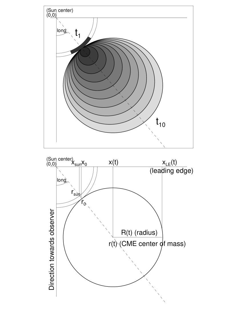
Figure 1: Geometric diagram of a spherically expanding CME (top) and definition of geometric parameters (bottom), along the plane-of-sky (x-axis) and the radial propagation direction (diagonal dashed line): $r_{sun}$ and $x_{sun}$ refer to photospheric (and projected) distance from Sun center, $r_{0}$ and $x_{0}$ to an altitude of one emission measure scale height in the corona, $r(t)$ and $x(t)$ to the center of mass of the CME, $x_{LE}(t)$ to the leading edge of the CME, $R(t)$ is the radius of the expanding CME, and $long$ is the longitudinal angle between the observer’s line-of-sight and the CME center-of-mass trajectory.

We start with a geometric model of the time-dependent CME volume as depicted in Fig. 1. Before the launch of the CME, all the plasma that will feed the later expanding CME volume is confined in a volume $V_{0}$ with an area $A=L^{2}$ (with an unprojected length scale $L$) on the solar surface, within a vertical height extent $h_{0}$ that corresponds to the temperature-dependent electron density scale height $\lambda_{n_{e}}(T_{e})$ observed at the beginning of the flare at temperature $T_{0}=T_{e}(t=t_{start})$,

$$V_{0}=L^{2}h_{0}=L^{2}\ \lambda_{n_{e}}(T_{0})\ ,$$ (1)

where the electron density scale height $\lambda_{n_{e}}$ is,

$$\lambda_{n_{e}}(T_{0})={2\ k_{B}\ T_{0}\over\mu\ m_{H}\ g_{\odot}}\approx 4.7\times 10^{9}\ \left({T_{0}\over 1\ {\rm MK}}\right)\quad[cm]\ .$$ (2)

where $k_{B}=1.38\times 10^{-16}$ erg K^-1 is the Boltzmann constant, $\mu\approx 1.27$ is the mean molecular weight, $m_{H}=1.67\times 10^{-24}$ g is the hydrogen mass, and $g_{\odot}=\Gamma M_{\odot}/R_{\odot}^{2}=2.74\times 10^{4}$ cm s^-2 is the solar gravity acceleration. This initially surface-aligned volume $V_{0}$ is shown from a top-down view for an equatorial CME at a longitudinal angle $\rho=l$ (between the observer’s line-of-sight and the CME center-of-mass trajectory) from the central meridian at time $t_{1}$ in Fig. 1 (top panel). For an arbitrary CME launch position the angle $\rho$ can be calculated from the heliographic position at longitude $l$ and latitude $b$ from spherical trigonometry,

$$\cos{(\rho)}=\cos{(l)}\cos{(b)}\ .$$ (3)

The top side of the pre-lauch CME volume at an altitude $h_{0}$ above the photosphere has a distance of

$$r_{0}=R_{\odot}+h_{0}\ ,$$ (4)

from Sun center, where $R_{\odot}$ is the solar radius, and the projected distance $x_{0}$ from Sun center in the plane-of-sky is (Fig. 1, bottom panel),

$$x_{0}=(R_{\odot}+h_{0})\sin{(\rho)}\ .$$ (5)

At the launch time $t=t_{1}$ of the CME, the plasma confined in the original volume $V_{0}=v(t\leq t_{1})$ will start to stream into a spherical volume that expands subsequently (as shown for 10 time steps from $t_{1}$ to $t_{10}$ in Fig. 1, top panel), where the bottom of the sphere stays connected at a coronal height $h_{0}$, and the CME center of mass moves in radial direction away from the Sun at the radial position $r(t)$, with a CME radius of $R(t)$ (Fig. 1, bottom panel),

$$R(t)=r(t)-r_{0}\ ,$$ (6)

The projected position $x(t)$ of the CME center of mass is

$$x(t)=r(t)\ \sin{(\rho)}\ ,$$ (7)

and the projected position $x_{LE}(t)$ of the CME leading edge is

$$x_{LE}(t)=x(t)+R(t)\ .$$ (8)

The projected leading edge position $x_{LE}(t)$ is important for relating the timing of the coronagraphic CME detection to the EUV dimming model. If a coronagraph detects a CME at a projected location $x_{LE}(t)$ at time $t$, it follows from Eqs. (6-8) that the radial distance $r(t)$ of the CME center-of-mass from Sun center is,

$$r(t)={r_{0}+x_{LE}(t)\over 1+\sin{(\rho)}}\ .$$ (9)

Thus the geometric CME model can be described with the time evolution of the radial distance $r(t)$ of the CME center-of-mass position from Sun center, the heliographic position $(l,b)$ of the flare (or CME launch) site, the (unprojected) length scale $L$ of the CME footpoint area, and with the emission measure-weighted temperature $T_{w}$ (which defines $h_{0}$, $r_{0}$, and $V_{0}$). The emission measure-weighted temperature $T_{w}$ can be determined from the differential emission measure distributions $dEM(T)/dT$ at the peak time of a flare,

$$T_{w}={\int T\ [dEM(T)/dT]\ dT\over\int[dEM(T)/dT]\ dT}\ ,$$ (10)

as described in Papers II and IV.

2.2 The CME Acceleration Phase

We define the start time $t_{1}$ of the CME acceleration phase by the time when the total emission measure profile $EM(t)$ peaks during a flare time interval. This follows from the fact that the time evolution of the EUV dimming has only a physical meaning when it decreases, which requires a temporal peak at the beginning of the EUV dimming phase. Thus the initial parameters at the beginning of the EUV dimming phase or before $(t\leq t_{1})$ are according to the geometric model depicted in Fig. 1,

$$(t\leq t_{1})\left\{\begin{array}[]{ll}a(t)&=0\\ v(t)&=0\\ r(t)&=h_{0}\\ R(t)&=0\\ x(t)&=x_{0}\\ \end{array}\right.$$ (11)

where $a(t)$ is the acceleration and $v(t)$ the velocity of the CME center of mass. We employ the simplest model for the CME acceleration phase, namely a constant acceleration $a$ during a time interval $\tau_{acc}$ (similar to Paper IV), i.e., $t_{1}\leq t\leq t_{2}$, defining an acceleration end time $t_{2}$ of

$$t_{2}=t_{1}+\tau_{acc}\ .$$ (12)

The time evolution of the dynamical parameters during this acceleration phase $t_{1}\leq t\leq t_{2}$ is thus,

$$(t_{1}\leq t\leq t_{2})\left\{\begin{array}[]{ll}a(t)&=a_{1}\\ v(t)&=a_{1}(t-t_{1})\\ R(t)&=(a_{1}/2)(t-t_{1})^{2}\\ r(t)&=r_{0}+(a_{1}/2)(t-t_{1})^{2}\\ \end{array}\right.$$ (13)

while the projected positions $x(t)$ and $x_{LE}(t)$ follow from Eqs. (7-8). At the end time $t_{2}$ of the acceleration phase, the values of the kinematic parameters are,

$$(t=t_{2})\left\{\begin{array}[]{ll}a_{2}=a(t=t_{2})&=a_{1}\\ v_{2}=v(t=t_{2})&=a_{1}(t_{2}-t_{1})=a_{1}\tau_{acc}\\ R_{2}=R(t=t_{2})&=(a_{1}/2)(t_{2}-t_{1})^{2}=(a_{1}/2)\tau_{acc}^{2}\\ r_{2}=r(t=t_{2})&=r_{0}+(a_{1}/2)\tau_{acc}^{2}\\ \end{array}\right.$$ (14)

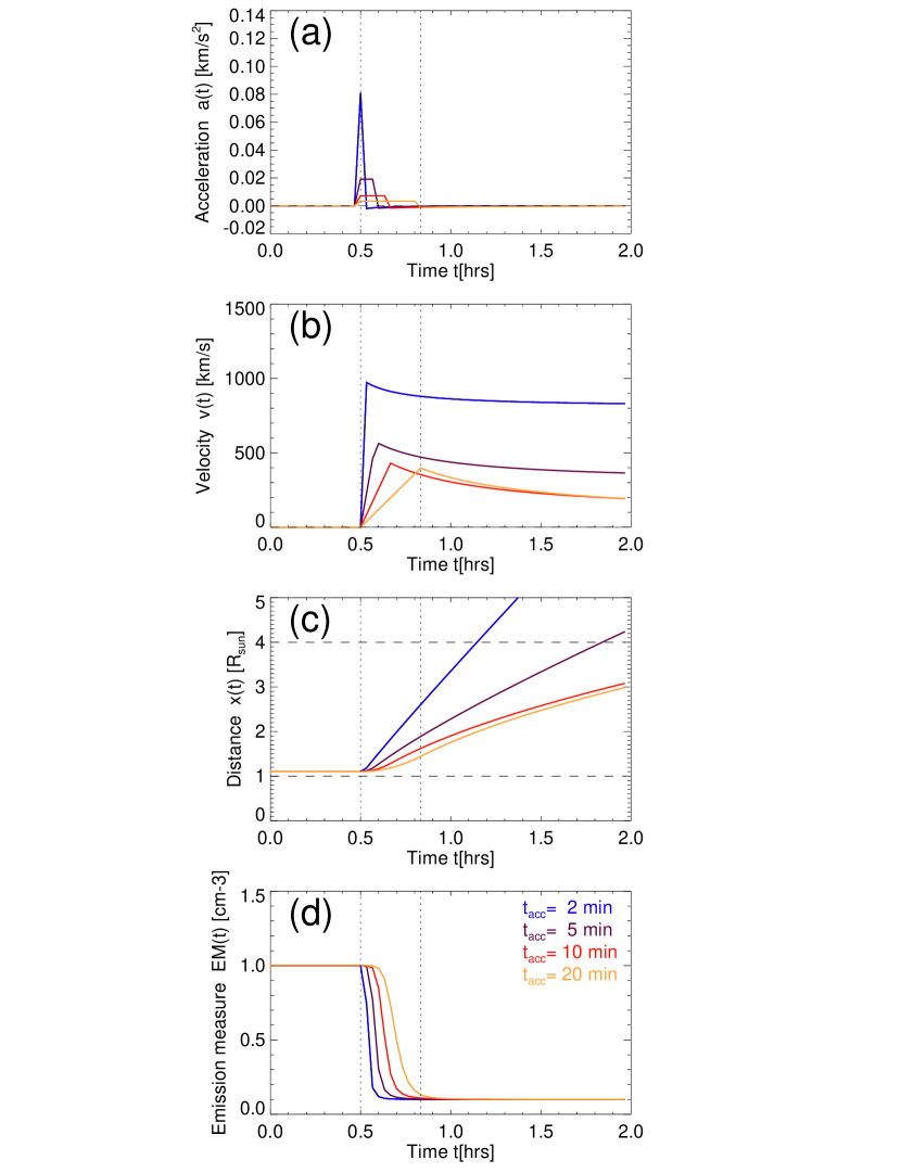
Figure 2: Time evolution of: (a) the acceleration $a(t)$, (b) the velocity $v(t)$, (c) the projected distance of the CME center-of-mass motion $x(t)$ (third panel), and (d) the total emission measure $EM(t)$, for four different acceleration time intervals ($\tau_{acc}=2,5,10,20$ min). The start $t_{1}$ and end time $t_{2}$ of acceleration is indicated with vertical dotted lines for the case of $\tau_{acc}=20$ min.

A graphic representation of the evolution of the acceleration $a(t)$, speed $v(t)$, and position $r(t)$ of the CME center of mass is shown in Fig. 2.

2.3 Gravitational Deceleration Phase

We define now a third time interval, $t>t_{2}$, when the CME is not accelerated any further, but is only subject to the deceleration $a(t)$ caused by the gravity force, which is important for CMEs that reach a speed near or below the escape speed from the Sun,

$$a(t)=-{\Gamma M_{\odot}\over r(t)^{2}}\ ,$$ (15)

where $\Gamma$ is Newton’s gravitational constant, and $M_{\odot}=2\times 10^{33}$ g is the solar mass. We see that this equation represents a second-order differential equation of the type $(r^{\prime\prime}r^{2}=const)$ that has no simple analytical solution. However, since the velocity becomes almost constant after the acceleration phase, we can approximate the time dependence of the radial distance with $r(t)\approx r_{2}+v_{2}(t-t_{2})$ to first order, which leads to the following time evolution of the gravitational deceleration,

$$a(t)\approx-\Gamma M_{\odot}[r_{2}+v_{2}(t-t_{2})]^{-2}\ ,$$ (16)

expressed as an explicit function of time. We can now calculate the time evolution of the CME center-of-mass speed straightforwardly by time integration of the deceleration (Eq. 16),

$$v(t)=v_{2}+\int_{t_{2}}^{t}a(t)\ dt=v_{2}-{\Gamma M_{\odot}\over v_{2}}\left\{{1\over r_{2}}-{1\over r_{2}+v_{2}(t-t_{2})}\right\}\ .$$ (17)

We see that the speed $v(t)$ is monotonically decreasing with time after $t>t_{2}$, and converges asymptotically to the final speed $v_{\infty}$ (at time $t\mapsto\infty$),

$$v_{\infty}=v(t=\infty)=v_{2}-{\Gamma M_{\odot}\over v_{2}\ r_{2}}\ .$$ (18)

Finally we can also calculate a more accurate value for the evolution of the radius $R(t)$ of the CME by time integration of the velocity $v(t)$ given in Eq. (17), using the integral $\int r^{-1}\ dr=\ln{(r)}$,

$$R(t)=R_{2}+\int_{t_{2}}^{t}v(t)\ dt=R_{2}+[v_{2}-{\Gamma M_{\odot}\over v_{2}r_{2}}](t-t_{2})+{\Gamma M_{\odot}\over(v_{2})^{2}}\left\{\ln{[r_{2}+v_{2}(t-t_{2})]}-\ln{[r_{2}]}\right\}\ .$$ (19)

The distance $r(t)$ of the CME center-of-mass from Sun center follows then (with Eq. 6),

$$r(t)=r_{0}+R(t)\ ,$$ (20)

and the projected position $x(t)$ of the CME center-of-mass and $x_{LE}(t)$ of the CME leading edge follow from Eqs. (7-8).

2.4 Confined and Escaping CMEs

The fate of whether the expanding CME sphere escapes during the eruption from the Sun, or whether it turns into a stalled (failed) eruption that comes to a halt and falls back to the Sun, depends on whether the CME reaches the critical escape velocity during the initial acceleration phase or not. Since our dynamic model is designed to reach a maximum speed $v_{2}$ at the end of the acceleration phase at $t=t_{2}$, which is $v_{2}=a_{1}\tau_{acc}$ (Eq. 14), the critical escape speed $v_{CME}$ has to be calculated at this position $r_{2}=r_{0}+(a_{1}/2)\tau_{acc}^{2}$ (Eq. 14), which follows from Eq. (18) by setting $v_{\infty}=0$, yielding with Eqs. (4) and (13),

$$v_{esc}(r=r_{2})=\left({2\Gamma M_{\odot}\over r_{2}}\right)^{1/2}=\left({2\Gamma M_{\odot}\over R_{\odot}+h_{0}+(a_{1}/2)\tau_{acc}^{2}}\right)^{1/2}\ .$$ (21)

Thus, our analytical model describes the time evolution of both a confined flare, if $v_{2}<v_{esc}(r_{2})$, and an eruptive CME, if $v_{2}\geq v_{esc}(r_{2})$.

2.5 Coronagraphic CME Detections

It is also useful to relate the CME velocity $v$ to the propagation distance $r$, which allows us to compare the speeds of our model with coronagraphic observations. From the conservation of kinetic energy and the gravitational potential at distances $r$ and $r_{2}$,

$${1\over 2}m_{cme}v^{2}-{1\over 2}m_{cme}(v_{2})^{2}=+{\Gamma M_{\odot}m_{cme}\over r}-{\Gamma M_{\odot}m_{cme}\over r_{2}}\ ,$$ (22)

we can obtain the velocity $v[r(t)]$ at any location $r(t)$ after the acceleration phase, at $t\geq t_{2}$,

$$v[r(t)]=\left[(v_{2})^{2}-2\Gamma M_{\odot}\left({1\over r_{2}}-{1\over r(t)}\right)\right]^{1/2}\ .$$ (23)

For instance, if a CME is detected with a coronagraph at time $t=t_{3}$ at a distance $x_{3}$ given by the occulting disk, which corresponds to a radial distance $r_{3}=(r_{0}+x_{3})/(1+\sin{(\rho))}$ from Sun center according to Eq. (9), we can predict the velocity $v_{3}$ at this particular location and time,

$$v_{3}=\left[(v_{2})^{2}-2\Gamma M_{\odot}\left({1\over r_{2}}-{1\over r_{3}}\right)\right]^{1/2}\ .$$ (24)

For LASCO observations for instance, the occulting disk is at $x_{3}=x_{LASCO}\approx 4R_{\odot}$, where the CME mass $m_{LASCO}$, the speed $v_{LASCO}$, and the detection time $t_{LASCO}$ is measured, which can then be compared with the values $m_{3},v_{3}$, and $t_{3}$ of our CME model. The predicted time $t_{3}$ of CME detection with LASCO can be computed in our CME model from the parameters $(r_{2},v_{2},v_{3})$ using Eq. (17),

$$t_{3}=t_{2}+\left({1\over v_{2}}\right)\left[\left({(v_{3}-v_{2})v_{2}\over\Gamma M_{\odot}}+{1\over r_{2}}\right)^{-1}-r_{2}\right]\ .$$ (25)

2.6 Adiabatic CME Expansion and EUV Dimming

Our dynamic CME model can be fitted to data that measure the EUV dimming, which requires the time evolution of the total emission measure $EM(t)$. In our simple CME model we assume a purley adiabatic expansion, where no energy is exchanged across the boundaries of a CME, and thus predicts that the average electron density changes reciprocally to the expanding CME volume (Paper IV), in order to conserve the number of particles,

$$q_{EM}(t)={EM(t)\over EM_{0}}={V_{0}\over V(t)}\ ,$$ (26)

where $EM_{0}$ and $V_{0}$ are the initial total emission measure and the initial volume (as defined in Eq. 1). Therefore, all that is needed to calculate the time evolution of the EUV dimming $EM(t)$ is the time-dependent volume $V(t)$, which we define as the sum of the coronal source volume $V_{0}$ and the spherically expanding CME volume,

$$V(t)=V_{0}+{4\over 3}\pi R(t)\ ,$$ (27)

where the CME radius $R(t)$ is defined with Eq. (13) during the acceleration phase, and with Eq. (19) after the acceleration phase, during gravitational deceleration.

Since there is always some background emission measure observed in every flare and CME, originating from the non-flaring part of the Sun, we have to correct the observed emission measure by the fraction of the background component $q^{bg}$,

$$EM^{fit}(t)=EM^{max}\left[q^{bg}+(q^{peak}-q^{bg})q_{EM}(t)\right]\ ,$$ (28)

where $EM^{max}$ is the maximum of the observed emission measure and $q^{peak}$ is the fraction of the modeled peak emission measure to the absolute maximum of the observed total emission measure. We see from Eq. (28) that the modeled emission measure has the initial value $EM^{fit}(t=t_{1})=EM^{max}q^{peak}$ (for $q_{EM}(t=t_{1})=1$), and asymptotically approaches the value $EM^{fit}(t=\infty)=EM^{max}q^{bg}$ (for $q_{EM}(t=\infty)\mapsto 0$).

2.7 Energy Equi-Partition Model

The observed EUV dimming exhibits the fastest change in the initial phase of the CME expansion (in the lower corona), while the later expansion in the heliosphere causes very small changes that asymptotically reach unmeasurable small values. The final CME speed is therefore very weakly constrained by the emission measure profile $EM(t)$. It is therefore desirable to test the final CME expansion speed $v(t)$ by other means, for instance by making use of the assumption of energy partition between the kinetic and thermal energy contained in the corresponding flare, which has been empirically found to be closely fulfilled in a previous statistical study (Paper V),

$$E_{kin}={1\over 2}m_{cme}v^{2}\approx E_{th}=3n_{e}k_{B}T_{w}V\ .$$ (29)

Since both forms of energy contain the volume-integrated CME mass, $m_{cme}=n_{e}m_{p}V$, both the density and the volume cancel out, and yields a very simple relationship between the CME velocity $v$ and the (emission measure-weighted) flare temperature $T_{w}$. If we apply this energy equi-partition to the maximum CME kinetic energy, which happens at $v_{2}=v(t=t_{2})$ in our model, we obtain

$$v_{2T}=\sqrt{\left({6k_{b}\over m_{p}}\right)\ T_{w}}=c_{1}\ \left({T_{w}\over 10\ {\rm MK}}\right)^{1/2}\qquad c_{1}=704\ {\rm km}\ {\rm s}^{-1}\ .$$ (30)

where we denote the velocity as $v_{2T}$ to indicate the temperature model. From our previous study we measured (emission measure-weighted) flare temperatures in the range of $T_{w}=3-14$ MK, for which the energy equi-partition model (Eq. 30) predicts maximum velocities in the range of $v_{2}=384-830$ km s^-1.

2.8 The Rosner-Tucker-Vaiana Scaling Law

A scaling law for the energy balance between the heating rate and the (conductive and radiative) cooling rate has been derived for quiescent coronal loops (Rosner et al. 1978), which applies also to the turnover point between the dominant heating phase and the dominant cooling phase in solar flares (Aschwanden and Tsiklauri 2009). The original formulation by Rosner et al. (1978) states the relationship $T_{max}\approx 1400(p_{0}L)^{1/3}$ between a loop apex temperature $T_{max}$, the approximately constant loop pressure $p_{0}$, and the half length $L$ of a semi-circular loop. Inserting the iso-thermal pressure of an ideal gas, $p=2k_{B}n_{e}T_{e}$, yields then a relationship for the electron density at the footpoints of flare loops (Aschwanden and Shimizu 2013, Eq. 14 therein),

$$n_{e}=n_{e0}\ \left({T_{e}\over 10\ {\rm MK}}\right)^{2}\left({L\over 10^{10}\ {\rm cm}}\right)^{-1}\qquad n_{e0}=8.4\times 10^{9}\ {\rm cm}^{-3}\ .$$ (31)

The geometry of a post-flare arcade is typically a sequence of semi-circular flare loops, which can be represented by a volume that covers the flare or CME footprint area $A=L^{2}$ and has a typical filling factor of $q_{fill}\approx 0.05$ for the Euclidean volume $V=L^{3}$ (Aschwanden and Aschwanden 2008b),

$$V=V_{0}\left({L\over 10^{10}\ cm}\right)^{3}\left({q_{fill}\over 0.05}\right)\ ,\qquad V_{0}=0.5\times 10^{29}\ {\rm cm}^{-3}\ .$$ (32)

The total CME mass (initially confined in the flare volume) is then,

$$m_{cme}=n_{e}\ m_{p}\ V_{0}=n_{e}\ m_{p}\ L^{2}h_{0}\ ,$$ (33)

where $m_{p}$ is the proton mass. Combining the Eqs. (31-33), together with the relationship of the equi-partition between the kinetic and thermal energy (Eq. 30) we obtain then a total mass of

$$\left({m_{cme}\over 10^{15}\ {\rm g}}\right)=0.7\ \left({T_{e}\over 10\ {\rm MK}}\right)^{2}\left({L\over 10^{10}\ cm}\right)^{2}\left({q_{fill}\over 0.05}\right)\ .$$ (34)

Expressing the CME velocity $v_{CME}=v_{2m}$ explicitly, we obtain the scaling law

$$v_{2m}=1.09\ c_{1}\left({m_{cme}\over 10^{15}\ {\rm g}}\right)^{1/4}\left({L\over 10^{10}\ {\rm cm}}\right)^{-1/2}\left({q_{fill}\over 0.05}\right)^{-1/4}\approx c_{2}\left({m_{cme}\over 10^{15}\ {\rm g}}\right)^{(1/4)}\ ,\qquad c_{2}=767\ {\rm km}\ {\rm s}^{-1}\ ,$$ (35)

where we denote the velocity with $v_{2m}$ to indicate the mass model. If we ignore the dependence on the loop length $L$ and the filling factor, we can approximately predict the maximum CME speed $v_{2}$ from the CME mass $m_{cme}$ alone. In our analyzed data set we find CME masses of $m_{cme}\approx(0.01-40)\times 10^{15}$ g, from which Eq. (35) predicts CME speeds in the range of $v_{2}\approx 200-1600$ km s^-1.

We have now two equi-valent relationships for the CME speed, one that depends only on the temperature, i.e., $v_{2T}=(T_{e}/10$ MK)^1/2 $\times 704$ km s^-1 (Eq. 30), and one that depends only on the CME mass, i.e., $v_{2m}=(m_{cme}/10^{15}$ g$)^{1/4}\times 767$ km s^-1 (Eq. 35). The difference between the two methods provides an estimate of systematic uncertainties. In our data analysis method we determine the maximum CME speed $v_{2}$ independently from the EUV dimming alone, without making the assumption of energy equi-partition or tht RTV law, but can use those assumptions as an additional test, besides comparisons of the speeds $v_{2}$ measured in white-light data from LASCO.

3 OBSERVATIONS AND DATA ANALYSIS

In a previous study (Aschwanden 2016; Paper IV), the kinematic parameters of CMEs have been modeled from the EUV dimming observed with AIA/SDO, and have been compared with the same parameters obtained from white-light data observed with LASCO/SOHO. In this study we present a refined CME model with extended data analysis, incorporating a number of additional effects (as enumerated at the beginning of Section 2) that were not taken into account in the previous study. The key parameters that we are interested in here are the CME mass, speed, and kinetic energy.

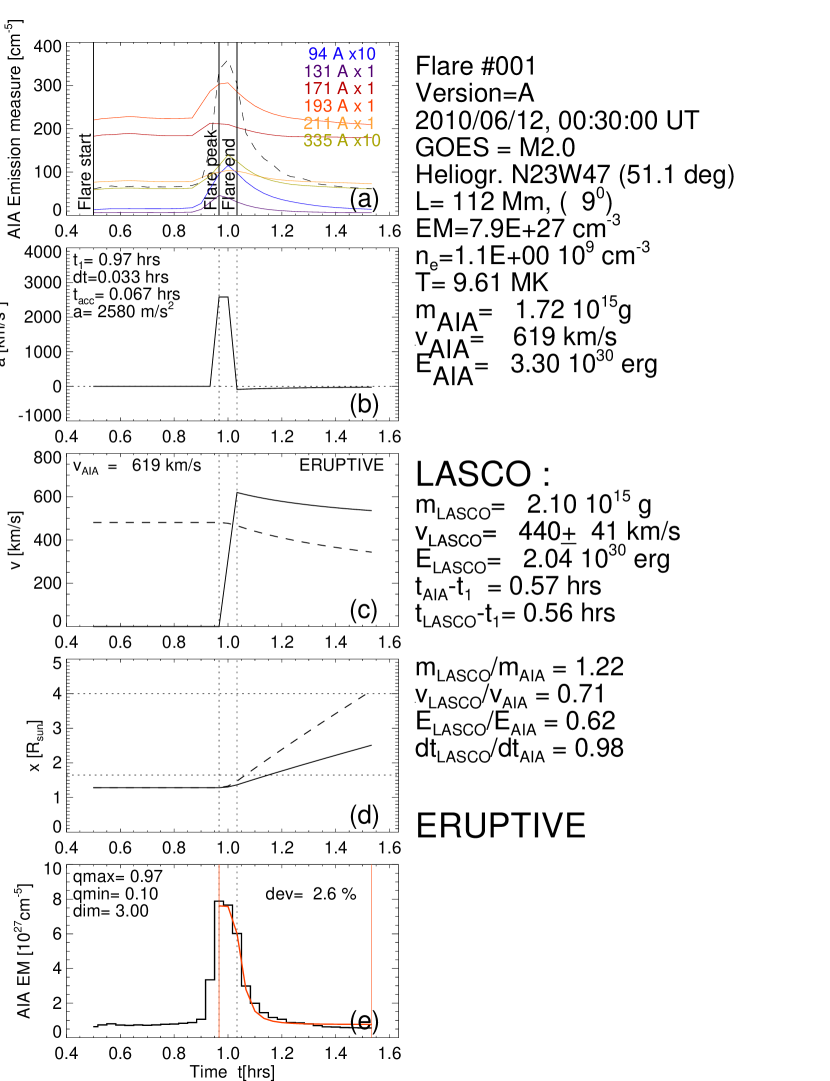
Figure 3: Example of data analysis (event #1), a GOES M2.0-class flare observed with AIA on 2010 June 12, 00:30 UT: (a) AIA light curves (colored) and total emission measure (dashed); (b) acceleration time profile, (c) CME speed (solid profile) and escape speed (dashed profile); (d) projected distance of CME center-of-mass (solid curve) and leading edge (dashed curve), with the initial CME height and LASCO coronagraph occultation height (dotted horizontal lines), and (e) total emission measure profile $EM(t)$ observed (black histogram) and modeled by forward-fitting (red thick curve), the fitting time interval (red lines), and end time of acceleration (dotted).

The analysis procedure is depicted in Fig. 3, which consists of the measurements of the fluxes in each AIA wavelength (Fig. 3a) and the DEM inversion of the total emission measure profile $EM(t)$ (Fig. 3e), which is fitted with the theoretical CME model (red profile in Fig. 3e) described in Fig. 2, yielding the CME motion at a projected distance $x(t)$ (Fig. 3d), the velocity profile $v(t)$ (Fig. 3c), and the acceleration profile $a(t)$ (Fig. 3b). In the following we describe the statistical distributions of the measured and best-fit physical CME parameters, displayed in form of power law distributions (Fig. 4) or Gaussian normal distributions (Fig. 5), from which we list the parameter ranges, medians, power law slopes, and means and standard deviations in Table 1.

3.1 AIA Observations

The analyzed data set includes all GOES M- and X-class flare events recorded during the first 7 years (June 2010 - Nov 2016) of the SDO mission, which amounts to 864 events, where we doubled the previously analyzed data set from the first 3.5 years of the SDO mission (Paper I-V). Only 4 events of the AIA data set contained data gaps during the flare time interval, which are discarded here, while 860 events remain for further analysis. We are using the same event numbering list as in Papers I-V, so the event numbers #1, …, #399 are identical with the previous analysis, while the events #400, …, #864 are new. The time evolution of the analyzed images is subdivided into steps of $\Delta t=2$ min, covering the entire flare duration as defined by the start and end times (prolonged by a margin of 30 min) from the GOES flare list.

3.2 Flare Temperatures

The first step in our analysis of AIA flare data is the automated differential emission measure (DEM) analysis, using the spatial-synthesis DEM code (Aschwanden et al al. 2013), which uses the 6 coronal AIA wavelengths (94, 131, 171, 193, 211, 335 Å) and yields a time sequence of DEM distributions $dEM(T,t)/dT$, as described in the previous Papers II and IV. From these DEMs we determine the emission measure-weighted flare temperatures $T_{w}(t)$ (Eq. 10) for each time step, and take then the maximum value $T_{w}=T_{w}(t=t_{max})$ of the time sequence to characterize the (thermal) density scale height near the flare peak. The distribution of these flare temperatures $T_{w}$ is shown in Fig. 5a, which covers a range of $T_{w}^{max}=2.3-17.4$ MK and has a mean of $T_{w}^{max}=9.3\pm 2.4$ MK. Note that this flare temperature range is substantially higher than the pre-CME temperatures $T_{e}=1.2-5.0$ MK determined in the previous study (Paper II), which define the CME volume and mass (Eqs. 1, 33).

3.3 CME Source Parameters

The source volume $V_{0}$ of the CME at the beginning of (or before) the expansion is defined in terms of the unprojected source area $A$ and the vertical height $h_{0}$ (Eq. 1). The measurement of the unprojected length scale $L$ is described in Section 2.3 in Paper IV, for which we find a range of $L=18-361$ Mm (Fig. 4a). The resulting CME footpoint or dimming area $A$ is simply defined as $A=L^{2}$ (Fig. 4b), where $L$ is the deprojected length scale.

The preflare temperature $T_{0}$ defines then the emission measure scale height $h_{0}=\lambda_{n_{e}}(T_{0})$ according to Eq. (2). The pre-flare temperature is measured at the start time $t_{start}$ of the GOES flare, which amounts to an average value of $T_{0}=1.8\pm 0.3$ MK (with a scale height $\lambda_{n_{e}}\approx 0.12\ R_{\odot}$). The peak of the flare temperature is found at a mean value of $T_{w}=9.3\pm 2.4$ MK (with a scale height $\lambda_{n_{e}}=0.63\ R_{\odot}$). The temperature at the time $t_{1}$ of the CME launch, defined by the start of the EUV dimming or peak value of the total emission measure, is generally between the GOES flare start $t_{start}$ and the temperature maximum time $t_{m}=t(T=T_{m})$, i.e., $t_{0}<t_{1}<t_{m}$, at an average temperature of $T_{m}=4.7\pm 1.2$ MK, with a (with a scale height $\lambda_{n_{e}}=h_{0}\approx 0.31\pm 0.08)R_{\odot}$ (Fig. 5b). The resulting CME source volumes (Eq. 1) of the analyzed 860 events vary in the range of $V_{0}=(0.0005-0.5)\times 10^{30}$ cm³ (Fig. 4c).

The maximum emission measure per area $EM(t)/A$ displays the most extended power law distribution (over two decades), with a power law slope of $p=-2.6\pm 0.6$ (Fig. 4d). The total emission measure is defined in terms of the spatially integrated emission measure $EM_{0}=EM(t=t_{1})$ at the emission measure peak time $t_{1}$. This yields the mean electron density in the CME source volume according to $n_{e}=\sqrt{EM_{0}/V}$. For the pre-flare or pre-CME phase, which serves to measure the CME mass, we find a very narrow distribution with a mean of $n_{e}=(1.2\pm 0.5)\times 10^{9}$ cm^-3 (Fig. 5c).

From the electron density $n_{e}$ and the CME source volume $V_{0}$ we can then directly calculate the CME mass with

$$m_{cme}=m_{p}n_{e}V_{0}\approx 0.81\times 10^{15}\ \left({L\over 10^{10}\ {\rm cm}}\right)^{2}\left({n_{e}\over 10^{9}\ {\rm cm}^{-3}}\right)\left({T_{0}\over 1\ {\rm MK}}\right)\quad[g]\ .$$ (36)

where we inserted the volume definition $V=L^{2}\lambda_{n_{e}}(T_{0})$ (Eq. (1), and $m_{p}$ is the proton mass. The distribution of CME masses is shown in form of power law distributions in Fig. (4e), which exhibits a total range of $m_{cme}=(0.07-31)\times 10^{15}$ g.

3.4 Fitting of Emission Measure Profile

The observed EUV dimming profile $EM(t)$ (e.g., Fig. 3e) exhibits generally a steep rise before the CME launch at time $t_{1}$ (defined by the peak time of the emission measure profile), which then monotonically drops afterwards, which we interpret as density upflow by chromospheric evaporation (during the rise of the total emission measure), followed by EUV dimming caused by adiabatic expansion of the CME volume (during the decay phase). Our theoretical model of adiabatic expansion (Eqs.26-28) can be fitted to the observed EUV dimming profile $EM(t)$ with four free parameters: the acceleration constant $a_{1}$, the acceleration start time $t_{1}$, the acceleration time interval $\tau_{acc}=t_{2}-t_{1}$, and the background fraction level $q_{bg}$. We fit these four free parameters to the EUV dimming profile $EM(t)$ for each event in a time range $[t_{f1},t_{f2}]$ (marked with red lines in Fig. 3), where the beginning of the fitting interval coincides with the peak of the emission measure, $t_{f1}=t_{1}$, and the end of the fitting interval is $t_{f2}=t_{1}+2\tau_{acc}$, which corresponds to the double duration of the acceleration time interval $\tau_{acc}$. This time interval $[t_{f1},t_{f2}]$ covers the steepest decrease of the EUV dimming profile in a symmetric way, where the detection of the dimming is most significant, while the dimming-related EUV emission drifts outside the field-of-view of the AIA images later on (at a distance of $\lower 1.72218pt\hbox{$\;\buildrel>\over{\scriptstyle\sim}\;$}1.3R_{\odot}$), a second-order effect that is not modeled here.

The distributions of the best-fit parameters is shown in Figs. 4 and 5, including the acceleration constant $a_{1}$ (Fig. 4g), the acceleration time interval $\tau_{acc}=$ (Fig. 4h), and the background fraction level $q_{bg}$ (Fig. 5f). the peak fraction level $q_{peak}$ (Fig. 5g), and the fit quality $q_{fit}$ (Fig. 5h), which is a measure of the mean deviation between the observed and modeled EUV emission measure, normalized by the maximum emission measure $EM_{max}$. The accuracy of the fits is typically 5% of the peak emission measure.

3.5 CME Acceleration Parameters

The most important fitting parameter is the acceleration time $\tau_{acc}$, which defines the end time $t_{2}$ of the acceleration phase and the distance $x_{2}$ (Eq. 14) of the CME at the time of maximum velocity $v_{2}=v(t=t_{2})$, when the acceleration stops and deceleration due to the solar gravity sets in. We can compare the best-fit parameters $v_{2}$ with those estimated from the energy equi-partition theorem, based on the flare temperature $v_{2T}(T_{w})$ (Eq. 30), or based on the CME mass $v_{2m}(m_{cme})$ (Eq. 35). The distributions of the velocities $v_{2T}$ and $v_{2m}$ are shown in Fig. (5d) and (5e), covering ranges of $v_{2T}=340-930$ km s^-2, and $v_{2m}=340-1540$ km s^-2, respectively (Table 1).

Having the acceleration time interval $\tau_{acc}=t_{2}-t_{1}$ and the maximum velocity $v_{2}$ established, we obtain immediately the acceleration rate, $a=v_{2}/\tau_{acc}$ (Eq. 14) and the acceleration height $h_{2}=r_{2}-R_{\odot}=r_{0}-R_{\odot}+(a/2)\tau_{acc}$ (Eq. 14), since we assumed constant acceleration during the acceleration phase in our model. The distributions or the acceleration rate ($a_{1}=0.24-10$ km s^-2) (Fig. 4g), the CME acceleration time ($\tau_{acc}=120-3360$ s), (Fig. 4h), and the acceleration height $h_{2}=(0.11-2.38)\times R_{\odot}$ (Fig. 4i), which all show power law-like distributions (over a relatively small range of 1.5 decades).

3.6 Eruptive and Confined CMEs

The time $t_{2}$ of maximum CME speed at distance $x_{2}$ is the earliest time when it can be decided whether the CME is eruptive or confined, simply by comparing the velocity $v_{2}$ with the local escape speed $v_{esc}(x_{2})$ (Eq. 21). The height dependence of the escape speed due to the $r^{2}$-dependence of the gravitational force is shown for one case in Fig. (3c), which varies from $v_{esc}(r_{0})\approx 550$ km s^-1 to $v_{esc}(r_{2})\approx 350$ km s^-1 at the height $r_{2}$ of maximum CME speed. The CME has a maximum velocity of $v_{2}=619$ km s^-2, and thus is eruptive in this case.

In our statistics of 860 CME events, we find 841 eruptive CME events, and 19 confined flares ($\approx 2.3\%$).

3.7 LASCO and AIA Event Association

For a comparison of AIA results with LASCO data of CMEs we have first to evaluate which events are associated. The primary time definition of the analyzed events comes from the GOES flare catalog, which defines a start, peak, and end time for each of the analyzed flare events.

The LASCO data are catalogued in a CME event list that is available online, https://cdaw.gsfc.nasa.gov/ CME$\_$list/, and their detection time is defined when the CME leading edge shows up the first time at the edge of the LASCO occulter disk at a distance of $x_{3}=4R_{\odot}$ from Sun center. The delay of the LASCO detection and the CME launch as detected by the EUV dimming in AIA data is expected to vary over a range of $t_{delay}=4R_{\odot}/v_{cme}\approx[0.4,4]$ hrs, for CME speeds in the range of $v_{cme}=[200,2000]$ km s^-1.

In Fig. 6a we show a histogram of the expected time delays $t_{AIA}$ based on our CME model described in Section 2, which exhibits a mean value of $t_{AIA}=0.39\pm 0.23$ hrs. An upper limit above 3 standard deviations would be around $t_{AIA}\lower 1.72218pt\hbox{$\;\buildrel<\over{\scriptstyle\sim}\;$}0.39+3\times 0.23=1.1$ hrs. On the other side, the histogram of time delays $t_{LASCO}$ observed with LASCO show a similar almost Gaussian distribution with a mean of $t_{LASCO}=0.44\pm 0.25$ hrs (Fig. 6b). If we fit a Gaussian function, we estimate an upper limit of $t_{LASCO}\lower 1.72218pt\hbox{$\;\buildrel<\over{\scriptstyle\sim}\;$}0.44+3\times 0.25\approx 1.2$ hrs. Since the CME propagation delay has to be positive by definition, we expect that the range of physical delays is bound by the range $t_{AIA}\approx t_{LASCO}\lower 1.72218pt\hbox{$\;\buildrel<\over{\scriptstyle\sim}\;$}1.0$ hrs. Most of the AIA events (828) are found in this range, while LASCO exhibits a smaller number of 432 CME detections inside this range (52 %). A scatterplot of the AIA and LASCO detection delays is shown in Fig. 6c, which shows a mean difference of $t_{AIA}-t_{LASCO}=0.05\pm 0.50$ hrs, which implies a slight systematic error in the inferred CME speeds (either from AIA, or LASCO, or both).

3.8 LASCO Outliers of CME Masses

We measure the CME mass here with two different methods, either with the conventional method based on the white-light polarized brightness in coronagraph images, or with the novel method using the EUV dimming. We were able to measure a EUV dimming effect, and therefore a CME mass, in all 860 flares from AIA/SDO data, while the white-light data from LASCO/SOHO reported a CME detection in about 432 events thereof.

We show a histogram of the CME masses obtained with LASCO in Fig. 7a, the corresponding CME masses inferred from AIA in Fig. 7b, and a scatterplot of the two types of masses in Fig. 7c. The range of LASCO-inferred CME masses covers a range of $m_{LASCO}=(0.01-37)\times 10^{15}$ g, and the AIA-inferred CME masses cover a narrower range of $m_{AIA}=(0.1-30)\times 10^{15}$ g. Thus the two ranges exhibit a very similar upper limit, but differ in the lower limit. It appears that LASCO under-estimates CME masses up to an order of magnitude. The sample of CME masses measured with AIA exhibits a sharp cutoff around $m_{cme}\approx 0.25\times 10^{15}$ g (dashed line in Fig. 7b, while LASCO reports CME masses smaller than this lower limit for 99 events. We inquired the LASCO CME catalog and found that most of these low-mass events were evaluated as “poor” or “very poor” quality in the LASCO CME event catalog. These poor events were identified near the LASCO detection threshold, which is likely to be the cause of under-estimating the CME mass. When we apply the same limit to the AIA-inferred masses, there is only one maverick event below $m_{AIA}=0.25\times 10^{15}$ g (see dashed lines in Fig. 7). So, there are three reasons why these low-mass cases obtained with LASCO data are likely to be outliers: (1) The fact that AIA detects no CME masses below the limit of $m_{cme}=0.25\times 10^{15}$ g; (2) AIA should detect lower CME masses because the EUV dimming method based on the total emission measure is more sensitive than the polarized brightness method in white light (because we detect EUV dimming in all of the joint 456 events, while LASCO detects CMEs unambiguously in 348 ($\approx 76\%$) events only; and (3) most of the low-mass LASCO events suffer from instrumental sensitivity problems (qualified as “poor” or ”very poor” events, mostly detected in the coronagraph C2 only). In the following analysis we will discard these low-mass outliers, which leaves 334 events for further LASCO and AIA comparisons.

We determine the average mass ratio between AIA and LASCO-inferred CME masses and find $m_{AIA}/$ $m_{LASCO}=0.92$, with a standard deviation factor of 3.6 of the logarithmically averaged masses (Fig. 7d). The lower mass limit apparently yields a closer agreement between the two instruments, because the ratio is less commensurate when the low-mass outliers are included. Applying the lower mass limit, the CME masses cover a range of $m_{cme}=(0.25-37)\times 10^{15}$ g, which corresponds to a mass variation by a factor of $\approx 150$. The cross-correlation coefficient between the LASCO and AIA-inferred CME masses is $CCC\approx 0.29$ (Fig. 7d), indicating a weak correlation due to the remaining methodical errors in modeling of the CME mass and the measurement of underlying parameters.

3.9 Scaling Laws of CME Parameters

The CME speed is traditionally measured with the white-light method from coronagraphic observations, typically at distances of a few solar radii when the CME emerges behind the occultation disk, e.g. at $x_{3}\lower 1.72218pt\hbox{$\;\buildrel>\over{\scriptstyle\sim}\;$}4R_{\odot}$ with LASCO. In contrast, the EUV dimming effect allows for measurements of the CME expansion speed in the lower corona, most sensitive at altitudes that correspond to one emission measure scale height. Extrapolating the time evolution of CME speeds to heliospheric distances as probed by coronagraphs, requires additional constraints.

In Section 2.7 we derived a prediction of the maximum speed based on the energy equi-partition model between the kinetic and the thermal flare energy, which predicts a relationship

$$v\propto T_{e}^{1/2}\ .$$ (37)

The scatterplot of CME speeds $v_{3}$ (calculated with the relationship of Eq. 24 at the coronagraphic occulter position $x_{3}=4R_{\odot}$) with the flare emission measure-weighted flare temperatures $T_{e}$ is shown in Figs. 8a (for LASCO speeds) and in Fig. 9a (for AIA speeds), which agree within factors of 1.7 and 2.3, respectively.

As an alternative model we employed the Rosner-Tucker-Vaiana scaling law (Section 2.8), which predicts a relationship between the CME mass and the flare temperature, which can be used to predict a relationship of the CME mass with the maximum CME speed, i.e.,

$$v\propto(m_{cme})^{1/4}\ .$$ (38)

We show a scatterplot of the CME velocity $v_{3}$ (calculated at location $x_{3}$ with Eq. 24) with the CME mass (raised to the power of 1/4) in Figs. 8b (for LASCO speeds) and Fig. 9b (for AIA speeds). We find a good agreement within a factor of 2.7 and 2.6, respectively. The cross-correlation coefficient is $CCC=0.62$ (Fig. 8b), which confirms that the RTV relationship indeed is physically related to the CME speed.

The correlations of LASCO and AIA CME speeds $v_{2}$ or masses $m_{cme}$ with the CME length scales $L$ are shown in Figs. 8c,d and Fig. 9c,d. The tightest correlation is found between the AIA-inferred CME mass and the CME length scale $L$, with a cross-correlation coefficient of $CCC=0.77$ (Fig. 9d), which reflects the scaling law of the RTV relationship between mass and length scale,

$$m_{cme}\propto L^{2}\ .$$ (39)

This scaling law follows from the definition of the CME mass, $m_{cme}\propto A^{2}h_{0}$ (Eq. 1), if the density scale height $h_{0}$ is constant or has only little variation.

These results allow us to use the RTV-based model as a prediction of the maximum CME speed $v_{2}$ for AIA data, solely based on the measurement of the CME mass from the EUV dimming, i.e., $v_{AIA}=767$ km s^-1 $\times(m_{cme}/10^{15}$ g)^1/4. Based on this formula, a velocity range of $v_{2}=540-1900$ km s^-1 is predicted by the RTV law.

3.10 Comparison of Old and New CME Model

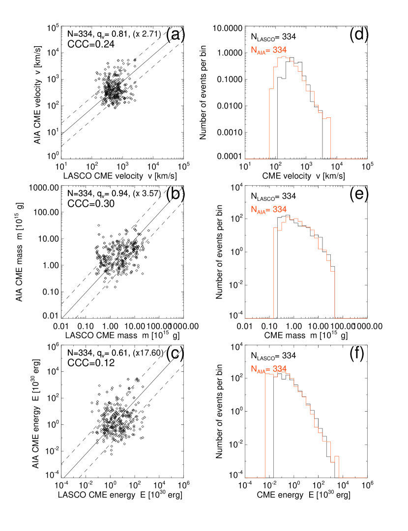
Figure 10: AIA-inferred versus LASCO-inferred parameters: (a) CME velocity, (b) CME mass, and (c) CME energy. The ratios $q_{v}$ are obtained from the logarithmic averages (indicated with a solid line), and the standard deviation factors are indicated with dashed lines. The corresponding size distributions (d,e,f) are displayed with a black histogram for the LASCO events, and with a red histogram for the AIA events.

A scatterplot of the CME parameters obtained with both instruments AIA and LASCO, which includes the CME speed ($v_{LASCO}$ vs. $v_{AIA}$), the CME mass ($m_{LASCO}$ vs. $m_{AIA}$), and the kinetic energy ($E_{LASCO}$ vs $E_{AIA}$), has been shown in Fig. 18 for 218 CME events in the previous Paper IV. We show the scatterplots of the same parameters obtained with the new method (Fig. 10, left panels), sampled after elimination of low-mass and mis-associated events, using the equi-partition assumption and the RTV scaling laws. The substantial scatter between the old and new method indicates significantly differences for individual events, but the resulting size distributions are similar (Fig. 10, right panels).

4 DISCUSSION

4.1 Measurements of Coronagraph-Detected CMEs

CMEs have traditionally been observed and measured with coronagraphs in white-light, such as with the Orbiting Solar Observatory OSO-7 (Tousey 1973), the Apollo Telescope Mount (ATM) onboard Skylab (Mac Queen et al. 1974), the Solwind coronagraph onboard P78-1 (Michels et al. 1980), the Coronagraph/Polarimeter (CP) onboard the Solar Maximum Mission (SMM) (House et al. 1980), the Large-Angle and Spectrometric Coronagraph (LASCO) (Brueckner et al. 1995), the Solar Mass Ejection Imager (SMEI) (Eyles et al. 2003), and the Sun Earth Connection Coronal and Heliospheric Investigation (SECCHI) onboard the Solar Terrestrial Relations Observatory (STEREO) with the two coronagraphs COR1 and COR2 (Howard et al. 2008). What could be measured with these coronagraphs is primarily the detection time $t_{cme}$ when the CME emerges from behind the coronagraph occulter disk, for instance at a distance of $x_{cme}\approx 4R_{\odot}$ for LASCO, their angular width $w_{cme}$, their mass $m_{cme}$ based on the polarized brightness produced by Thomson scattering, and their projected speed measured in the field-of-view of the coronagraphs. Once the mass $m_{cme}$ and the speed $v_{cme}$ is known, their kinetic energy $E_{kin}=(1/2)m_{cme}(v_{cme})^{2}$ can directly be obtained.

Catalogs of CME events observed with LASCO have been published and are available on websites, such as the LASCO/CDAW catalog https://cdaw.gsfc.nasa.gov/CME$\_$list/, the LASCO-based Computer Aided CME Tracking (CACTUS) catalog http://sidc.oma.be/cactus (Robbrecht and Berghmans 2004; Robbrecht et al. 2009), the LASCO-based Solar Eruptive Event Detection System (SEEDS) catalog (Olmedo et al. 2008), and the LASCO-based Coronal Image Processing (CORIMP) catalog (Byrne et al. 2012; Morgan et al. 2012). While these catalogs are all based on LASCO-detected events, there are also CME measurements using the STEREO/COR2 instrument given in the SEEDS and CACTUS catalogs.

What are the strengths and weaknesses of the coronagraph-based measurements of CMEs? The foremost advantages of coronagraphic measurements are: (1) The uninterrupted long-term availability over 20 years (since the launch of SOHO in 1996); (2) the derivation of the CME mass is independent of the temperature; (3) the measurement of the projected leading-edge CME speed is well-defined and can be automated (for instance with the Hough transform; Robbrecht and Berghmans 2004). On the other side, there are a number of disadvantages that makes the EUV dimming method truly complementary: (4) The association of CMEs with flare events is often ambiguous; (5) The kinematics or the evolution of the height $h(t)$, the velocity $v(t)$, and acceleration $a(t)$ in the source region is not known in the altitude range where a CME is occulted by the coronagraph disk (at $x_{3}\lower 1.72218pt\hbox{$\;\buildrel<\over{\scriptstyle\sim}\;$}1.6-4.0R_{\odot}$); and (6) the magnetic topology and plasma temperature diagnostics in the CME source region cannot be deduced from white-light data; (7) Projection effects in halo CMEs make it difficult to disentangle the kinematics and 3D geometry of Earth-directed CMEs. All these deficiencies make it also difficult to derive 3D models of CMEs that cover the entire evolution from the source region in the lower corona out to the heliosphere, which is a necessary pre-requisite to test data-driven MHD simulations and theoretical models of CMEs.

4.2 Measurements of CMEs from EUV Dimming

Measurements of CME parameters from EUV dimming information started with the availability of solar EUV images, such as with the EUV Imaging Telescope (EIT) onboard SOHO since 1996 (e.g., Thompson et al. 2000), the Extreme Ultra-Violet Imager (EUVI) onboard STEREO since 2006 (e.g., Bein et al. 2011), and the Atmospheric Imager Assembly (AIA) onboard SDO since 2010 (e.g., Cheng et al. 2012; Mason et al. 2014; Kraaikamp and Verbeek 2015; Aschwanden 2016, Paper IV). Dimming regions were identified by areas of strong depletion in the EUV brightness, mapping out the apparent “footpoint” area of a CME, which is detected with a white-light coronagraph generally about an hour later (Thompson et al. 2000). Consequently, a high association rate of $\approx 55-74\%$ was found between EUV dimming and CME events (Bewsher et al. 2008; Nitta et al. 2014). The 3D structure of CME source regions and the associated EUV dimming could be modeled with stereoscopic methods (Aschwanden et al. 2009a,b; Aschwanden 2009; Temmer et al. 2009; Bein et al. 2013). A key result was that the CME mass determined from EUV dimming agreed well with those determined with the white-light scattering method ($m_{\mathrm{EUVI}}/m_{\mathrm{LASCO}}=1.1\pm 0.3$), and agreed also between the two STEREO spacecraft A and B ($m_{A}/m_{B}=1.3\pm 0.6$) (Aschwanden et al. 2009a). Another benefit of stereoscopic observations is the determination of the 3D trajectory and de-projected CME speed and mass (Bein et al. 2013).

Systematic measurements of the main physical parameters of EUV dimming events and associated CMEs started only recently, amounting to a statistical study of 399 events during the first 3.5 years of the SDO mission (2010-2014; Paper IV), which we expand here to 864 events during the first 7 years of the SDO mission. The basic measurements consist of the decreasing slope in the total emission measure profile of the EUV brightness $EM(t)$ during a flare, which can be modeled with a spatially expanding CME volume $V(t)$ and the assumption of an adiabatic process. In the simplest scenario, the time evolution of the CME volume is reciprocal to the mean electron density, $n_{e}(t)\propto V(t)^{-1}$, which can be related to the volume-integrated emission measure by $EM(t)\propto n_{e}(t)^{2}V(t)$ for optically thin plasmas. In the previous study (Paper IV), the velocity of the expanding CME volume was derived from forward-fitting of the systematically decreasing emission measure profile $EM(t)$ after the flare peak, which turned out to be strongly disturbed by multiple brightenings immediately followed by dimming episodes in large and complex flare events. Hence, we developed a new method in this study where the CME velocity is determined from the equi-partition between kinetic CME velocity and the thermal flare energy, which predicts a simple relationship between the CME velocity and the flare temperature, $v_{cme}\propto(T_{w})^{1/2}$. The emission measure-weighted flare temperature can directly be obtained from the DEM distribution of the flare region obtained with an automated algorithm in the flare/dimming region (Aschwanden et al. 2013). Moreover, we derived a redundant method where the RTV scaling law is applied to the flare loops at the peak time (turnover point) when the heating rate and the cooling rate is balanced, which yields a simple relationship between the CME velocity and the CME mass, $v_{cme}\propto(m_{cme})^{1/4}$. With these new developments we obtained a CME model that is completely based on EUV dimming data and can predict all CME white-light parameters as well as additional CME model parameters with unprecedented robustness.

4.3 CME Acceleration and Deceleration

Our CME model provides a powerful tool to diagnose acceleration and deceleration phases of CMEs. Acceleration can be caused by the magnetic pressure term of the Lorentz force, a pressure gradient, and the solar wind flow, while deceleration can be caused by the Sun’s gravity, the aerodynamic drag, and the tension of the magnetic field, as studied by 3D MHD simulations (e.g., Shen et al. 2012).

There is an increasing number of observational studies available now that provide statistical information on CME acceleration. The range of of acceleration rates is quite different near the Sun, typically $a_{max}\approx 100-2000$ m s^-2 (e.g., Zhang and Dere 2006; Cheng et al. 2010; Bein et al. 2011; Joshi and Srivastava 2011), compared with the heliosphere, say in the LASCO field-of-view at $r\lower 1.72218pt\hbox{$\;\buildrel>\over{\scriptstyle\sim}\;$}4R_{\odot}$, where it can be positive or negative, typically in a range of $a=\pm 20$ m s^-2 (e.g., Michalek 2012). For the solar gravity force alone we would expect a deceleration of $a=-\Gamma M_{\odot}/(4R_{\odot})^{2}\approx-17$ m s^-1 at the inner boundary of the LASCO field-of-view.

How does our EUV dimming model complement previous measurements of CME acceleration and deceleration? Our AIA-constrained dimming model can fill in the gaps of measurements below the coronagraph occultation height (say at $r\lower 1.72218pt\hbox{$\;\buildrel<\over{\scriptstyle\sim}\;$}4R_{\odot}$ for LASCO), which contains the most important height range for studying the magnitude and duration of magnetic Lorentz forces that accelerate the CME. Secondly, the AIA-constrained method yields the total emission measure, which contains all particle contributions in the temperature range of $T_{e}\approx 0.5-20$ MK, so that the particle number is almost completely conserved, similar to the white-light Thomson scattering method, and thus heating or cooling processes do not interfere with the detection of EUV dimming. The broad AIA temperature coverage also constrains the emission-measure weighted temperature in the flare region, which is found here to be a good predictor of the maximum CME speed (Eq. 30). Furthermore, our analytical EUV-dimming model allows us to measure the duration and magnitude of the acceleration rate, as well as the gravity-driven deceleration, which are the most dominant force components for weak CMEs propagating near the escape speed.

4.4 Confined and Eruptive CMEs

Since both acceleration and gravity-driven deceleration is built in our analytical model, we should be in a good position to discriminate between eruptive and confined CMEs. For our analyzed data set of 860 flare events we found only 19 events (2.3%) to be confined flares. This is a relatively low percentage, compared with other studies. For instance, Cheng et al. ( 010) analyzed a sample of 1246 flare events and found that 706 events (57%) are associated with CMEs, while the other 540 flares (43%) are confined. The discrepancy may be related to the detection method. Cheng et al. (2010) did a visual inspection of the movies observed by LASCO and EIT/SOHO and identified CME-associated flare events if the spatio-temporal co-registration of transient flare brightenings and large-scale dimming on EIT images occurs. That means that confined flares are defined by the absence of spatio-temporal coincidences. It is not clear why this method produces a 25 times higher fraction of confined flares than our method of calculating the maximum CME speed and comparing it with the co-spatial escape speed. Nevertheless, such discrepancies provide important tests to sort out methodical biases in the data analysis and modeling of CMEs.

5 CONCLUSIONS

In this study we refined the method of calculating physical parameters of CMEs based on the EUV-dimming method, which provides a complementary approach to the traditional white-light method. An extensive study that compares the two strategies of white-light scattering and EUV dimming in the measurement of CME parameters has been undertaken in the previous Paper IV of this series on the global energetics of solar flares and CMEs. Here we focus on the improvements between the previous EUV dimming method (Paper IV) and the refined method presented in this study. The methodical improvements and related conclusions are summarized in the following.

1. Larger Statistics: By extending our analysis from the first 3.5 years of the SDO mission (with 399 events) to the currently entire SDO era of 7 years (2010-2016) (with 864 events) doubles the size of the statistical data sample (containing M and X-class flare events) investigated here, for both the AIA/SDO and LASCO/SOHO data sets. Most previous studies apply CME models to small samples of observed CMEs only and are therefore not statistically representative.

2. The Spatial CME Geometry: is given by self-similar (adiabatic) 3-D expansion of a spherical volume in the refined model, while the old model assumed the self-similar 1-D expansion of a wedge. The 3D spherical geometry appears to be more realistic, based on the observation of bubble-like CME geometries on one side, and the plausibility of isotropic expansion in coronal regions with a low plasma-beta parameter on the other side.

3. The Gravity Force: causes a deceleration of the expanding CME, which has been neglected in the old model (since it is not important for fast and large CMEs with speeds in excess of the escape speed. Inclusion of the gravitational force during the acceleration of CMEs, in contrast, is important for small CMEs (associated with M-class flares or lower) and can reproduce the dynamical behavior of “failed” CMEs properly, which allows the discrimination between eruptive and confined CMEs. We find that a fraction of 2.3% of CMEs (of $\geq$M1.0 GOES class) is associated with confined flares.

4. Speed Comparisons of CMEs: between traditional white-light observations (where the speed is specified at the leading edge) and EUV-dimming observations (where the speed is measured from the center-of-mass motion) need to be self-consistently modeled. The spherical self-similar expansion model implies a factor of 2 difference in the speeds of the center-of-mass motion and the leading-edge motion. The resulting corrections amount to a factor of 4 in the kinetic energies (since $E_{kin}\propto v^{2}$).

5. The association of LASCO and AIA CMEs: can only be properly determined if the time difference between the flare onset in the lower corona (coincident with the lauch of a CME) and the first detection in white-light outside the occultation disk of a coronagraph is measured and kinematically modeled. We find that the typical delay for LASCO observations (beyond an occultation disk with a radius of $r_{occ}\lower 1.72218pt\hbox{$\;\buildrel>\over{\scriptstyle\sim}\;$}4r_{\sun}$) is $\Delta t\approx 1.0$ hr.

6. LASCO is less sensitive than AIA in detecting small CME events. We estimate that LASCO detects $\approx 50\%$ of the AIA EUV dimming events (of $\geq M1.0$ GOES class).

7. The equi-partition between the CME kinetic energy and the thermal flare energy yields a simple scaling law between the (emission measure-weighted) flare temperature and the CME speed, i.e., $v_{2T}\propto T_{w}^{1/2}$, which provides a robust estimate for extrapolated CME speeds at heliospheric distances (within a factor of $\approx 2$). The equivalence of CME energies and thermal energies has also been established in a previous study (Paper V), where the CMEs were found to dissipate $E_{cme}/E_{mag}=0.07\pm 0.14$ of the magnetic energy (in the statistical mean of 157 events), while the thermal energy owns a ratio of $E_{th}/E_{mag}=0.08\pm 0.13$ in 170 events (Table 3 in Paper V), which implies an equi-partition of $E_{cme}/E_{th}=1.0\pm 0.2$ between the CME kinetic and thermal energy.

8. The Rosner-Tucker-Vaiana (RTV) law, which is based on the equi-partition of heating and cooling rates at the flare peak times yields two simple scaling laws, one between CME mass and the CME velocity, i.e., $v\propto m_{cme}^{1/4}$, and one between CME masses and CME footpoint area $A=L^{2}$, i.e., $m_{cme}\propto L^{2}$. Both scaling laws can be used to provide estimates of CME parameters (within a factor of $\approx 2$).

9. LASCO is under-estimating CME masses: in 24% of CME events associated with $\geq$M1.0 class flares. From AIA measurements we estimate that LASCO-inferred CME masses below a limit of $m_{cme}\lower 1.72218pt\hbox{$\;\buildrel<\over{\scriptstyle\sim}\;$}10^{14}$ g represent under-estimates.

In summary, the chief advantage of the EUV-dimming method described and refined in this study is the independent corroboration of the traditional white-light method to quantify basic physical parameters of CMEs. Since both methods have unknown systematic errors, the statistical comparison of the two independent methods can elucidate and quantify model uncertainties and systematic errors. The fact that both the white-light and the EUV dimming model agree in the determination of CME masses and speeds (within a factor of $\approx 3$) gives us confidence on the statistical consistency of both methods, which helps us also to identify outliers or the parameter space where the models break down. For instance, CME masses below a limit of $m_{cme}\lower 1.72218pt\hbox{$\;\buildrel<\over{\scriptstyle\sim}\;$}10^{14}$ g appear to be systematically under-estimated with the white-light method. Moreover, the EUV dimming method appears to be more sensitive than the white-light method for small events ($\;\buildrel>\over{\scriptstyle\sim}\;$M1 GOES class). The superior sensitivity of CME detection using EUV-dimming data enables us to measure CME parameters with AIA/SDO in many cases where the white-light method using LASCO/SOHO data is not available or is affected by ambiguous timing in the flare association. Future case studies of individual events with inconsistent CME parameters (obtained with either the white-light or the EUV-dimming method) may give us further insights where present CME models can be improved.

Table 1: Ranges and distributions of CME parameters measured in 860 CME events with AIA. The mean and standard deviations refer to the slopes $p$ of power law distributions, or to the Gaussian normal distributions $x\pm\sigma_{x}$.

Parameter	Range	Median	Physical	Distribution	Mean and
			Units	type	standard
					deviation
Length scale $L$	$(18,...,361)\times 10^{8}$	$99\times 10^{8}$	cm	power law	$p=-3.7\pm 1.2$
CME dimming area $A$	$(0.03,...,13)\times 10^{16}$	$1.0\times 10^{16}$	cm2	power law	$p=-2.9\pm 0.8$
CME dimming volume $V$	$(0.0005,...,0.5)\times 10^{30}$	$0.02\times 10^{30}$	cm3	power law	$p=-2.8\pm 0.7$
CME emission measure $EM/A$	$(13,...,3342)\times 10^{26}$	$84\times 10^{26}$	cm-5	power law	$p=-2.6\pm 0.6$
CME mass $m$	$(0.07,...,31)\times 10^{15}$	$1.54\times 10^{15}$	erg	power law	$p=-2.5\pm 0.6$
CME energy $E$	$(0.076,...,227)\times 10^{30}$	$3.66\times 10^{15}$	erg	power law	$p=-1.6\pm 0.2$
Acceleration rate $a_{1}$	$(0.24,...,10)$	1.43	km s-2	power law	$p=-1.7\pm 0.2$
Acceleration time $\tau_{acc}$	$(120,...,3360)$	480	sec	power law	$p=-2.6\pm 0.6$
Acceleration height $h_{2}$	$(0.11,...,2.38)$	0.56	$R_{\odot}$	power law	$p=-6.7\pm 2.5$
Preflare temperature $T_{0}$	$(1.2,...,5.0)$	1.8	MK	Gaussian	$T_{0}=1.8\pm 0.3$
Flare peak temperature $T_{w}$	$(2.3,...,17.4)$	8.9	MK	Gaussian	$T_{w}=9.3\pm 2.4$
EM scale height $h_{0}$	$(0.08,...,0.59)$	0.30	$R_{\odot}$	Gaussian	$h_{0}=0.31\pm 0.08$
Electron density $n_{e}$	$(0.28,...,6.8)\times 10^{9}$	$1.1\times 10^{9}$	cm-3	Gaussian	$n_{e}=(1.2\pm 0.5)\times 10^{9}$
CME max. speed $v_{2T}$	$(340,...,930)$	665	km s-1	Gaussian	$v_{2T}=670\pm 90$
CME max. speed $v_{2m}$	$(336,...,1542)$	766	km s-1	Gaussian	$v_{2m}=590\pm 66$
Background fraction $q_{bg}$	$(0.00,...,0.68)$	0.33		Gaussian	$q_{bg}=0.22\pm 0.12$
Peak fraction $q_{peak}$	$(0.69,...,1.0)$	0.92		Gaussian	$q_{peak}=0.89\pm 0.08$
Goodness-of-fit $q_{fit}$	$(0.00,...,0.24)$	0.05		Gaussian	$q_{fit}=0.07\pm 0.15$

Figure 4: Power law-like size distributions of physical parameters in CMEs.

Figure 5: Histogram of physical CME parameters and numerical fitting parameters with Gaussian-like distributions.

Figure 6: Histograms of the CME coronagraphic detection delay between the start of EUV dimming detected in AIA and the detection with LASCO at a distance of $x_{3}=4R_{\odot}$ from Sun center: (a) predicted from the AIA-inferred CME model; (b) observed with LASCO, and (c) cross-correlation plot. A gaussian function is fitted to the histograms.

Figure 7: (a) Logarithmic histograms of CME masses from LASCO and (b) from AIA, (c) scatter plot of AIA-inferred versus LASCO-inferred CME masses, (d) with the LASCO under-estimated cases removed. The CME lower mass limit at $m\geq 0.3\times 10^{15}$ is indicated (vertical dashed lines), as well as logarithmic average ratios (diagonal solid lines) with one standard deviation factors (diagonal dotted lines).

Figure 8: Predicted scaling laws tested with LASCO data. The datapoints of joint LASCO and AIA events ($N=334$) are marked with diamonds, a linear regression fit with a dotted line, and the theoretical scaling law prediction with a a solid black line (predicted in absolute terms without adjustment).

Figure 9: Predicted scaling laws tested with AIA data. The datapoints of joint LASCO and AIA events ($N=334$) are marked with diamonds, a linear regression fit with a dotted line, and the theoretical scaling law prediction with a a solid black line (predicted in absolute terms without adjustment).

References

- (1)
- (2)
- (3) Aarnio, A.N., Stassun, K.G., Hughes, W.J., and McGregor,S.L. 2011, Solar Phys. 268, 195.
- (4) Aschwanden, M.J. and Aschwanden, P.D. 2008, ApJ 674, 544.
- (5) Aschwanden, M.J., Nitta, N.V., Wuelser, J.P., Lemen, J.R., Sandman, A., Vourlidas, A., and Colaninno, R.C. 2009a, ApJ 796, 376.
- (6) Aschwanden, M.J., Wuelser, J.P., Nitta, N.V., and Lemen, J.R. 2009b, Solar Phys. 256, 3.
- (7) Aschwanden, M.J. 2009, Ann.Geophys. 27, 1.
- (8) Aschwanden, M.J. and Tsiklauri D. 2009, ApJSS 185, 171.
- (9) Aschwanden, M.J. and Shimizu, T. 2013, ApJ 776, 132.
- (10) Aschwanden, M.J., Xu, Y., and Jing, J. 2014, ApJ 797, 50, [Paper I].
- (11) Aschwanden, M.J., Boerner, P., Ryan, D., Caspi, A., McTiernan, J.M., and Warren, H.P. 2015, ApJ 802, 53, [Paper II].
- (12) Aschwanden, M.J., Holman, G.D., O’Flannagain, A., Caspi, A., McTiernan, J.M., and Kontar, E.P. 2016, ApJ 832, 27, [Paper III].
- (13) Aschwanden, M.J. 2016, ApJ 831, 105, [Paper IV].
- (14) Aschwanden, M.J., Caspi,A., Cohen, C.M.S., Holman, G.D., Jing, J., Kretzschmar, M., Kontar, E.P., McTiernan, J.M., Mewaldt, R.A., O’Flannagain, A., Richardson, I.G., Ryan, D., Warren, H.P., and Xu, Y. 2017, ApJ 836:17, [Paper V].
- (15) Bein, B.M., Berkebile-Stoiser, S., Veronig, A.M., Temmer, M., Muhr, N., Kienreich, I., Utz, D., and Vrsnak, B. 2011, ApJ 738, 191.
- (16) Bein, B.M., Temmer, M., Vourlidas, A., Veronig, A. M., and Utz, D. 2013, ApJ 768, 31.
- (17) Bewsher, D., Harrison, R.A., and Brown, D.S. 2008, A&A 478, 897.
- (18) Brueckner, G.E., Howard, R.A., Koomen, M.J., Korendyke, C.M., Michels, D.J., Moses, J.D., Socker, D.G., Dere, K.P., Lamy, P.L., Llebaria, A., Bout, M.V., Schwenn, R., Simnett, G.M., Bedford, D.K., and Eyles, C.J. 1995, Solar Phys. 162, 357.
- (19) Byrne, J.P., Morgan, H., Habbal, S.R., and Gallagher, P.T. 2012, ApJ 752, 145.
- (20) Chen, P.F. 2011, Living Rev. Solar Phys. 8, 1.
- (21) Cheng, X., Zhang, J., Saar, S.H., and Ding, M.D. 2012, ApJ 761, 62.
- (22) Cheng, X., Zhang, J., DIng, M.D., and Poomvises, W. 2010, ApJ 712, 752.
- (23) Eyles C.J., Simnett G.M., Cooke M.P., Jackson B.V., Buffington A., Hick P.P., Waltham N.R., King J.M., Anderson P.A., Holladay P.E. 2003, Solar Phys 217, 347.
- (24) Gao, P.X., Li, K.J., and Xu, J.C. 2011, Solar Phys. 273, 117.
- (25) Gopalswamy, N. 2016, Geoscience Letters 3:8.
- (26) Joshi, A.D. and Srivastava, N. 2011, ApJ 739, 8.
- (27) House, L.L., Wagner W.J., Hildner E., Sawyer C., Schmidt H.U. 1980, ApJ 244, L117.
- (28) Howard, R.A., Moses, J.D., Vourlidas, A., Newark, J.S., Socker, D.G., Plunkett, S.P., and 40 co-authors 2008, SSRv 136, 67.
- (29) Hundhausen, A.J. 1993, JGR 98, 13177.
- (30) Kraaikamp, E. and Verbeek, C. 2015, J. Space Weather Space Clim. 5, A18.
- (31) Lemen, J.R., Title, A.M., Akin, D.J., Boerner, P.F., Chou, C., Drake, J.F., Duncan, D.W., Edwards, C.G., et al. 2012, Solar Phys. 275, 17.
- (32) MacQueen, R.M., Eddy, J.A., Gosling, J.T., Hildner, E., Munro, R.H., Newkirk, G.A., Jr., Pland,A.I. and Rose,C.L. 1974, ApJ 187, L85.
- (33) Mason, J.P., Woods, T.N., Caspi, A., Thompson, B.J., and Hock, R.A. 2014, ApJ 789, 61.
- (34) Michalek, G. 2012, Solar Phys. 276, 277.
- (35) Michels, D.J., Howard R.A., Koomen M.J., Sheeley N.R. Jr. 1980, in Radio Physics of the Sun, (eds. Kundu, M.R. and Gergely, T.), D. Reidel, Dordrecht, p.439.
- (36) Morgan, H., Byrne, J.P., and Habbal, S.R. 2012, ApJ 752, 144.
- (37) Moon, Y.J., Choe, G.S., Wang, H., Park, Y.D., Gopalswamy, N., Yang, G., and Yashiro, S. 2002, ApJ 581, 694.
- (38) Nitta, N.V., Aschwanden, M.J., Freeland, S.L., Lemen, J.R., Wülser, J.P., and Zarro, D.M. 2014, Solar Phys. 289, 1257.
- (39) Olmedo, O., Zhang, J., Wechsler, H., Poland, A., Borne, K. 2008, Solar Phys. 248, 485.
- (40) Pesnell, W.D., Thompson, B.J., and Chamberlin, P.C. 2011, SP 275, 3.
- (41) Robbrecht, E., and Berghmans D. 2004, A&A 425, 1097.
- (42) Robbrecht, E., Patsourakos, S., and Vourlidas, A. 2009, ApJ 701, 283.
- (43) Rosner, R., Tucker, W.H., and Vaiana, G.S. 1978, ApJ 220, 643.
- (44) Schwenn,R., Raymond, J.C., Alexander,D., Ciaravella,A., Gopalswamy,N., Howard,R., Hudson,H., Kaufmann,P., et al. 2006, SSRv 123, 127.
- (45) Shen, F., Wu, S.T., Xueshang, F., and Wu, C.C. 2012, JGR Space Physics 117/A11, CiteID A11101.
- (46) Temmer, M., Preiss, S., and Veronig, A.M. 2009, Solar Phys. 256, 183.
- (47) Thompson, B.J., Cliver, E.W., Nitta, N., Delannee, C., and Delaboudiniere, J.P. 2000, GRL 27/10, 1431.
- (48) Tousey, R. 1973, in Space Research XIII, (eds. Rycroft, M.J., and Runcorn, S.K.), Akademie Verlag, Berling, p. 713.
- (49) Wang, Y., Chen, C., Gui, B., Shen, C., Ye, P., and Wang, S. 2011, JGR (Space Physics), 116, 4104.
- (50) Webb, D.F. and Howard, T.A. 2012, Living Rev. Solar Phys. 9, 3.
- (51) Yashiro, S., Akiyama, S., Gopalswamy, N., and Howard, R.A. 2006, ApJ 650, L143.
- (52) Yurchyshyn, V.B., Yashiro,S., Abramenko,V., Wang,H., and Gopalswamy,N. 2005, ApJ 619, 599.
- (53) Zhang, J. and Dere, K.P. 2006, ApJ 649, 1100.